ELECTROMAGNETIC DESIGN OF ACCELERATOR MAGNETS · 2009-08-03 · ELECTROMAGNETIC DESIGN OF ACCELERATOR MAGNETS S. Russenschuck CERN, 1211 Geneva 23, Switzerland Abstract Analytical

ELECTROMAGNETIC DESIGN OF ACCELERATOR MAGNETS

S. RussenschuckCERN, 1211 Geneva 23, Switzerland

AbstractAnalytical and numerical field computation methods for the design of conven-tional and superconducting accelerator magnets are presented. This report isan extract from a continuously updated eBook that can be downloaded fromhttp://russ.home.cern.ch/russ.

1 Guiding fields for charged particles

A charged particle moving with velocityv through an electro-magnetic field is subjected to the Lorentzforce according to

F = q(v ×B + E). (1)

While the particle moves from the locationr1 to r2 with v = drdt , it changes it’s energy by

∆E =∫ r2

r1

Fdr = q

∫ r2

r1

(v ×B + E)dr . (2)

The particle trajectorydr is always parallel to the velocity vectorv. Therefore the vectorv × B isperpendicular todr, i.e., (v × B) dr = 0. The magnetic field cannot contribute to a change in theparticle’s energy. However, if forces perpendicular to the particle trajectory are needed, magnetic fieldscan serve for guiding and focusing of particle beams. At relativistic speed, electric and magnetic fieldshave the same effect on the particle trajectory ifE ≡ cB. A magnetic field of 1 T is then equivalentto an electric field of strengthE = 3 · 108 V/m. A magnetic field of one tesla strength can easily beachieved with conventional magnets (superconducting magnets on an industrial scale can reach up to 10T), whereas electric field strength in the giga volt / meter range are technically not to be realized. This isthe reason why for high energy particle accelerators only magnetic fields are used for guiding the beam.Assuming a constant circular motion on the bending radiusr = R (also called the radius of gyration)gives

p = mv0 = qBzR . (3)

In charged particle dynamics it is customary to refer to the “momentum”pc which has the dimensionof an energy and to express it in units ofGeV. With q expressed in units of the electronic charge, theparticle momentum in GeV/c is determined by:

pGeV/c ≈ 0.3qeRm BzT. (4)

The termBzR is called the magnetic rigidity and is a measure of the beams “stiffness” in the bendingfield. In circular proton machines the maximum energy is basically limited by the strength of the bendingmagnets. According to Eq. (4) the trajectory radius of the particle increases with the particle momentum.As both the maximum field and the maximum dimensions of the magnets are limited, the magnetic fieldmust be ramped synchronously with the particle energy. Note that the effective radius is between 60% and70% of the tunnel radius because of the dipole “filling factor” (space needed for focusing quadrupoles,interconnection regions, cavities etc.) and the straight parts around the collision points.

411

2 Conventional and superconducting magnets

Fig. 1 left, shows the conventional dipoles for the LEP (Large Electron Positron collider) and the singleaperture dipole model used for testing the dipole coil manufacture for the LHC. The field calculationswere performed with the CERN field computation program ROXIE. The field representations in the ironyokes are to scale, the size of the field vectors changes with the different field levels. The maximummagnetic induction in the LEP dipoles is about 0.13 T. In order to reduce the effect of remanent ironmagnetization, the yoke is laminated with a filling factor of only 0.27. It can be seen that the field isdominated by the shape of the iron yoke.

If the excitational current is increased above a density of about 10A/mm2, superconductingtechnology has to be employed. Neglecting the quantum-mechanical nature of the superconductingmaterial, it is sufficient to notice that the maximum achievable current density in the superconductingcoil is by the factor of 500 higher than in copper coils. At higher field levels the field quality in theaperture is increasingly affected by the coil layout. Notice the large difference between the field in theaperture (8.3 T) and the field in the iron yoke (max. 2.8 T), which has merely the effect of shielding thefringe field.

3 Field quality in accelerator magnets

The quality of the magnetic field is essential to keep the particles on stable trajectories for about 108 turns.The magnetic field errors in the aperture of accelerator magnets can be expressed as the coefficients of theFourier-series expansion of the radial field component at a given reference radius (in the 2-dimensionalcase). In the 3-dimensional case, the transverse field components are given at a longitudinal positionz0 or integrated over the entire length of the magnet. For beam tracking it is sufficient to consider thetransverse field components, since the effect of the z-component of the field (present only in the magnetends) on the particle motion can be neglected. Assuming that the radial component of the magnetic fluxdensityBr at a given reference radiusr = r0 inside the aperture of a magnet has been measured orcalculated as a function of the angular positionϕ, we get for the Fourier-series expansion of the field

Br(r0, ϕ) =∞∑

n=1

(Bn(r0) sinnϕ+An(r0) cosnϕ), (5)

0.00 0.15 -0.15 0.29 -0.29 0.44 -0.44 0.59 -0.59 0.73 -0.73 0.88 -0.88 1.03 -1.03 1.18 -1.18 1.33 -1.33 1.47 -1.47 1.62 -1.62 1.77 -1.77 1.92 -1.92 2.06 -2.06 2.21 -2.21 2.36 -2.36 2.50 -2.50 2.65 -2.65 2.8-

|Btot| (T)

0.00 0.15 -0.15 0.29 -0.29 0.44 -0.44 0.59 -0.59 0.74 -0.74 0.88 -0.88 1.03 -1.03 1.18 -1.18 1.32 -1.32 1.47 -1.47 1.62 -1.62 1.77 -1.77 1.91 -1.91 2.06 -2.06 2.21 -2.21 2.36 -2.36 2.50 -2.50 2.65 -2.65 2.8-

|Btot| (T)

Fig. 1: Magnetic field strength in the iron yoke and field vector presentation of accelerator magnets. Left: C-Core dipole

(N · I = 2× 5250 A , B1 = 0.13 T) with a filling factor of the yoke laminations of 0.27. Right: LHC single aperture coil test

facility (N · I = 480000 A , B1 = 8.33 T). Notice that even with increased field in the aperture the field strength in the yoke

is reduced in the cosΘ magnet design.

2

R. RUSSENSCHUCK

412

with

An(r0) =1π

∫ π

−πBr(r0, ϕ) cosnϕdϕ, (n = 1, 2, 3, ...) (6)

Bn(r0) =1π

∫ π

−πBr(r0, ϕ) sinnϕdϕ. (n = 1, 2, 3, ...) (7)

If the field components are related to the main field componentBN we get withN = 1 for the dipole,N= 2 for the quadrupole, etc.:

Br(r0, ϕ) = BN (r0)∞∑

n=1

(bn(r0) sinnϕ+ an(r0) cosnϕ). (8)

TheBn are called thenormaland theAn theskewcomponents of the field given in tesla,bn the normalrelative, andan the skew relative field components. They are dimensionless and are usually given in unitsof 10−4 at a 17 mm reference radius. In practice theBr components are calculated in discrete pointsϕk = kπ

P − π, k =0,1,2,..,2P -1 in the interval[−π, π) and a discrete Fourier transformation is carriedout, i.e., for the normal component:

Bn(r0) ≈1P

2P−1∑k=0

Br(r0, ϕk) sinnϕk. (9)

The expression of field quality through the field components is perfectly in line with magnetic measure-ments using so-called harmonic coils, where the periodic variation of flux in radial or tangential rotatingcoils is analyzed with a Fast Fourier Transformation (FFT).

Consider a so-called tangential coil as sketched in Fig. 2 (left) rotating in the aperture of a magnet.With ϕ = ωt+ Θ, whereω is the angular velocity, the flux linkage through the coil at timet is given by

Φ(t) = NL

∫ ϕ+δ/2

ϕ−δ/2Br(rc, ϕ)rcdϕ

=∞∑

n=1

2NLrcn

sin(nδ

2)[Bn(rc) sin(nωt+ nΘ) +An(rc) cos(nωt+ nΘ)], (10)

r c = 1 7 m m

C o i l 1

C o i l 2

C e r a m i c s h a f t

x

y

C o i l 3

d

w t w t x

y

r 2 = 2 0 . 2 m m r 1 = 8 . 7 m m C o i l 1

C o i l 3

C o i l 2

Fig. 2: Left: Cross-section of the long ceramic measuring shaft for the LHC magnets with the three tangential coils centered

and aligned with ceramic pins. Right: Radial coil assembly.

3


413

whereN is the number of turns in the rotating coil,rc is the coil radius,L is the length of the rotatingcoil, δ is the opening angle of the coil andΘ is the positioning angle att = 0. The voltage signal at timet is then

U(t) = −dΦdt

=∞∑

n=1

2NLrcω sin(nδ

2)[−Bn(rc) cos(nωt+ nΘ) +An(rc) sin(nωt+ nΘ)] . (11)

With the geometric parameters of the measurement coil resulting in a constant factor (which can becalculated and calibrated) the field harmonics can be obtained by means of the FFT of the voltage signal.

4 Maxwell’s equations

In this section we will present Maxwell’s equations in global and integral form, and in the form ofclassical vector-analysis. For the solving of Maxwell’s equations in various circumstances we furtherneed the constitutive equations as well as the boundary and interface conditions. After a study of theproperties of soft and hard magnetic materials we will be able to approximately calculate the main fieldin conventional accelerator magnets. We first summarize the governing laws of electromagnetism in theirglobal form for all geometrical objects at rest.

Vm(∂a) = I(a) +ddt

Ψ(a) , (12)

U(∂a) = − ddt

Φ(a) , (13)

Φ(∂V ) = 0 , (14)

Ψ(∂V ) = Q(V ) . (15)

Eq. (12) is Ampere’s magnetomotive force law and Eq. (13) is Faraday’s law of electromagnetic induc-tion. Eq. (14) is the magnetic flux conservation law and Eq. (15) is Gauss’ fundamental theorem ofelectrostatics. In SI units,U denotes the electric voltage[U ] = 1 V andVm the magnetomotive force[Vm]= 1 A along the boundary∂a of a surfacea. The electric flux through the boundary surfacea = ∂V of avolumeV , is denotedΨ with [Ψ] = 1 C = 1 A·s, the magnetic flux is denotedΦ with [Φ] = 1 Wb = 1 V·s.I is the electric current[I] = 1 A across the surfacea. Q is the electric charge in a volumeV , [Q] = 1 C= 1 A·s. In integral form, Maxwell’s equations read for the stationary case in SI units:∫

∂aH · ds =

∫aJ · da +

ddt

∫aD · da, (16)∫

∂aE · ds = − d

dt

∫aB · da, (17)∫

∂VB · da = 0, (18)∫

∂VD · da =

∫VρdV. (19)

The vector fieldsE(t, r),H(t, r) are the electric and magnetic field intensities,D(t, r),B(t, r) are theelectric and magnetic induction (or flux density),J(t, r) is the electrical current density. These vec-tor fields are assumed to be finite in the entire domain and to be continuous functions of position andtime. Discontinuities in the field vectors may occur, however, on surfaces with an abrupt change ofthe physical properties of the medium. Such discontinuities must therefore be excluded until we havetreated the interface conditions in Section 7. The field intensitiesE andH are integrated along a line,[E] =1 V/m, [H] =1 A/m, whereas the flux and current densitiesD, B andJ are integrated over asurface,[D] =1 A·s/m2, [B] =1 V·s/m2, [J] =1 A/m2. The electric charge densityρ is integrated on a

4

R. RUSSENSCHUCK

414

volume,[ρ]= 1 As/m3. The field intensity vectors and the flux density vectors have different natures. Theline integrals ofE andH are the electric voltage and magnetomotive force, respectively. The surfaceintegrals ofD,B,J are the electric flux, the magnetic flux and the electric current across the surface.

As long as the necessary conditions (continuously differentiable vector fields, smooth surfaceswith simply connected, closed, piecewise smooth and consistently oriented boundary, volumes withpiecewise smooth, closed and consistently oriented surface) hold for the application of the Stokes andGauss theorem which read ∫

acurlg · da =

∫∂a

g · ds , (20)∫V

div g dV =∫

∂Vg · da , (21)

and if we assume that the surfaces and volumina are at rest, the field equations can be written as follows:∫acurlH · da =

∫a(J +

∂

∂tD) · da, (22)∫

acurlE · da = −

∫a

∂

∂tB · da, (23)∫

Vdiv BdV = 0, (24)∫

Vdiv DdV =

∫VρdV. (25)

The equations can only be true for arbitrary volumes and surfaces if the following equation hold for theintegrands:

curlH = J + ∂tD, (26)

curlE = −∂tB, (27)

div B = 0, (28)

div D = ρ. (29)

This is the classical vector analytical form of Maxwell’s equations. The use of notation∂t instead of∂∂t is a way to establish∂t as an operator on the same footing as the differential operatorsgrad,divandcurl. Eq. (26) - (29) are Maxwell’s equations in classical vector notation which is mainly due toO. Heaviside who eliminated the vector-potential and the scalar potential in Maxwell’s original set ofequations. Divergence free vector fields such as the magnetic induction are said to besolenoidal.

From the first Poincare lemma,div curlg = 0, it follows directly that

div(J + ∂tD) = div J + ∂tρ = 0 (30)

which is called the conservation of charge law. The commutation of thediv and∂t operators is admissibleif the fields and charge distributions are smooth. The law can be written in integral form as∫

∂VJ · da +

ddt

∫VρdV = 0 (31)

or in global form as

I(∂V ) +ddtQ(V ) = 0 . (32)

5


415

If at every point within a volumeV the charge density is constant in time we get

div J = 0 , (33)∫∂V

J · da = 0 , (34)

I(∂V ) = 0 , (35)

the latter being known as Kirchhoff’s node-current law applied in network analysis.

5 Constitutive equations

Maxwell’s equations constitute two vector equations (2× 3 equations) and two scalar equations (all-together 8 equations) for the unknownE,D,H,B,J andρ (16 unknowns). If we also consider that Eq.(28) follows from Eq. (27), then Maxwell’s equations can only be solved with the additional 9 materialrelations which are called theconstitutiveequations

B = µH, D = εE, J = κE, (36)

whereµ, ε,κ are the permeability[µ] = V·sA·m , the permittivity[ε] = A·s

V·m and the conductivity[κ] = AV·m ,

respectively. (The international IEC standard recommends to use the symbolσ for the conductivity whichis, however, also used for the surface charge density. Therefore we use the symbolκ as proposed in DIN1324). These most simple forms of constitutive equations hold only for linear (field independent), ho-mogeneous (position independent), isotropic (direction independent) and stationary media. The materialparameters may, however, depend on the spatial position.

If the physical properties in a specimen are the same in all directions, the material is said to beisotropic. In this case it is customary to express the permeability and permittivity as a function of thefree space (vacuum) field constants withµ = µrµ0 and ε = εrε0 whereµ0 = 4π · 10−7 H/m andε0 = 8.8542... · 10−12 F/m. The permeability and the permittivity of free space are related throughthe velocity of light in vacuum by

c0 =1

√ε0µ0

= 299 792 458 m/s . (37)

In a more general case, e.g., with a permanent magnetic or electric polarization (which are volume den-sities of magnetic and electric dipole moments, respectively) it will prove convenient to introduce newvectors; the electric polarizationPel and the magnetic polarizationPmag. Often the magnetic polariza-tion is replaced by themagnetizationM in units of A/m. The material relations can then be expressedas

B = µ0H + Pmag(H) = µ0(H + M(H)) , (38)

D = ε0E + Pel(E) . (39)

Note that the definition of the magnetization is not unique in literature and sometimesM containsµ0.

The polarization vectors are associated with matter and vanish in free space. For linear isotropicmaterial the polarization vectors are parallel to the field vectors and are found to be proportional accord-ing toPel = χeε0E andM = χmH so that for magnetic materials

B = µ0H + µ0χmH = µ0(1 + χm)H = µ0µrH = µH, (40)

whereµr = 1 + χm is the relative permeability,[µr] = 1E andχm is called magnetic susceptibility[χm] = 1E.

6

R. RUSSENSCHUCK

416

- g r a dd i v

c u r l

- g r a dd i v

c u r lA

B HE

q

D

f

mek

0

0

f

m

J

d t

- d t

Fig. 3: Maxwell’s “House” [3] with scalar and vector-potential as well as the material relations. Left facade: Faraday complex.

Right facade: Maxwell’s complex. Front facade: Electric fields and charges. Rear facade: Magnetic fields and impressed

currents. Note how Ohm’s law and the absence of free magnetic charges spoils the otherwise perfect symmetry.

6 Maxwell’s “House”

Employing the second Lemma of Poincare we can express the magnetic field by means of a magneticvector potential

B = curlA, (41)

as the magnetic flux density is source free. IfB in Eq. (27) is replaced bycurlA one obtainscurl(E +∂tA) = 0 and therefore the electric field can be expressed as

E = −gradφ− ∂tA. (42)

In the electrostatic case with∂t = 0 the electric field is curl free (irrotational),curlE = 0, and henceE = −gradφ . Since thecurl of the magnetic flux density is, in general, non-zero, it cannot always bewritten as the gradient of a scalar potential function. If, however, a vector-fieldT is found such that

curlT = J , (43)

then the vector fieldH−T is curl free, i.e.,curl(H−T) = 0 and thereforeH can be expressed as

H = −gradφredm + T . (44)

T is called the electric vector potential in the context of the so-calledT−Ω method for steady-state fieldproblems andφred

m is the reduced magnetic scalar potential. Several options for the choice ofT exist, [7].The most straight forward one is to use the Biot-Savart fieldHs computed from the impressed currentdistribution. The structure of the Maxwell equations and the electromagnetic potentials is revealed in aconstruction called Maxwell’s “House” in [3]. The house is displayed in Fig. 3.

For magneto(quasi)static problems with vanishing time derivative (∂t = 0) only the back facadeof Maxwell’s house remains standing erect. Maxwell’s equations reduce to

curlH = J, (45)

div B = 0 , (46)

with the constitutive equation

B = µH . (47)

7


417

7 Boundary and interface conditions

Subsequently, the closed domain (either 2D or 3D) in which the electromagnetic field is to be calculatedwill be denoted asΩ. The field quantitiesB andH satisfy boundary conditions on the piecewise smoothboundaryΓ = ∂Ω of the domainΩ, see Fig. 4.

Two types of boundary conditions, prescribed on the two disjoint smooth boundaries denotedΓH

andΓB with Γ = ΓH ∪ ΓB, cover all practical cases:

On the partΓB of the boundary the normal component of the magnetic flux density is prescribed.On symmetry planes parallel to the field, on far boundaries, or on outer boundaries of iron yokes sur-rounded by air (where it can be assumed that no flux leaves the outer boundary) the normal componentof the flux density (denotedBn) is zero. In some special cases the distribution ofBn can be estimatedalong a physical surface, e.g., the flux distribution in the air gap of an electrical machine can be assumedto be sinusoidal. These boundary conditions can be written in the form

Bn = B · n = σmag onΓB, (48)

whereσmag is the surface density of a fictitious magnetic charge. A surface charge is defined as a chargewith infinite density, while the charge per unit surface remains finite: Consider a thin layer of thicknessd in which a charge of densityρmag is present, see Fig. 5 left. In some surface∆x∆y of this layer thetotal charge∆Q = ∆x∆ydρmag is present which isdρmag per unit surface. If we letρmag → ∞ andd→ 0 so thatdρmag remains finite, we get the surface charge with the densityσmag = dρmag, [σmag] =1 V·s/m2.

On the partΓH of the boundary the tangential components of the magnetic field are prescribed. Inmany cases (as on symmetry planes perpendicular to the field) and on infinitely permeable iron poles,where the field enters at right angle, the tangential components of the field (denotedHt) are zero. Thetangential components ofH can also be determined by a real or fictitious surface current density. Allthese boundary conditions can be written in the form

H× n = α onΓH, (49)

whereα is the density of a real or fictitious electric surface current. A surface current is defined as acurrent with infinite density on a surface, while the current per unit length remains finite: Consider a thinlayer of thicknessd in which a current of densityJ flows, see Fig. 5 right. In some length∆l of thislayer flows the total current∆I = Jd∆l which isJd per unit length. If we letJ → ∞ andd → 0 sothatJd remains finite, we get the surface current with the densityα = Jd, [α] = 1 A/m. The condition

Ω1

Ω2 µ0

µ2

n1

n2Γ12

ΓH

ΓB

ΓH

ΓB

Fig. 4: Composite material domain with boundary and interface.

8

R. RUSSENSCHUCK

418

∆x

∆y ∆l

∆Q∆I

d d

Fig. 5: Left: Surface charge. Right: Surface current.

that the tangential components are zero on the boundary implies

Ht = 0 → n× (H× n) = 0 . (50)

In order to establish the interface conditions on a smooth surface (outer oriented by a given crossingdirection) between two regions with different magnetic properties, consider two domainsΩ1 with per-meabilityµ1 andΩ2 with permeabilityµ2 as shown in Fig. 6.

Consider a surface element which penetrates the interface and where the vectorda lies in theinterface plane, as shown in Fig. 6, left. Applying Ampere’s law

∫∂a H ·ds =

∫a J ·da to the rectangular

loop while letting the heightδ → 0 yields∫c(H2 ·

n2 × dada

−H1 ·n2 × da

da)ds =

∫cα · da

dads . (51)

Eq. (51) holds for any curvec, if the integrands obey

(H2 −H1) ·n2 × da

da= α · da

da, (52)

(H2 −H1)× n2 · da = α · da . (53)

Eq. (53) holds for any surface elementda in the plane of the interface. It yields

α = (H2 −H1)× n2 = (H1 −H2)× n , (54)

c

Γ12

µ2µ2

µ2

Ω2Ω2Ω2

µ1

Ω1

Ω1

n2n1

dan2 × da

n

nn

da2

da1

Bt2

B2

α2

Bn2

Bt1 B1

α1

Bn1

δ

δ

Fig. 6: Interface conditions for permeable media.

9


419

where the surface normal vectorn points fromΩ2 to Ω1 as shown in Fig. 6. If no real or fictitiouselectric surface currents exist, the tangential components of the magnetic field strength are continuous atthe interface

Ht1 = Ht2 ≡ (H1 −H2)× n = 0 . (55)

Now consider the volume of the “pill-box” as shown in Fig. 6 middle. With the flux conservation law∫∂V B · da = 0 which holds for any closed simply connected surface we get forδ → 0,∫

aσmagda =

∫aB1 · da1 + B2 · da2 =

∫a(B1 −B2) · n1da . (56)

Eq. (56) holds for any surfacea if the integrands obey

σmag = (B1 −B2) · n . (57)

If no fictitious magnetic surface charge density exists, the normal component of the magnetic flux densityis continuous at the interface

Bn1 = Bn2 ≡ (B1 −B2) · n = 0 . (58)

For a boundary of isotropic materialsfree of surface currents(Fig. 6 right) it follows that

tanα1

tanα2=

Bt1Bn1

Bt2Bn2

=µ1Ht1

µ2Ht2=µ1

µ2, (59)

at all pointsx ∈ Γ12. Forµ2 µ1 it follows thattanα2 tanα1. Therefore for all anglesπ/2 > α2 >0 we gettanα1 ≈ 0. The field exits vertically from a highly permeable medium into a medium withlow permeability. We will come back to this point when we discuss ideal pole shapes of conventionalmagnets, see Section 12.

Remark: Both B andH are discontinuous atx ∈ Γ12 and thereforecurlH anddivB cease tomake sense there. For any boundary value problem defined onΩ to bewell posed, the interface conditionshave to be implied. Ways of doing so include weak formulations in the Finite Element technique.

8 Magnetic anisotropy in laminated iron yokes

In case of anisotropic magnetic material the permeability has the form of a diagonal rank 2 tensor, so thatB = [µ]H with

[µ] =

µx 0 00 µy 00 0 µz

. (60)

In many materials, such as in rolled metal sheets, the fabrication process produces some regularity inthe crystal structure and consequently a dependence of the magnetic properties on the direction. Themost well known (and strongest) anisotropy in magnetic materials can be achieved by laminating theiron yokes. Between each of the ferromagnetic laminations of thicknesslFe (magnetically isotropic tofirst order) there is a non-magnetic (µ = µ0) layer of thicknessl0, as shown schematically in Fig. 7.

Consider a lamination in z-direction and the field componentsBt in thexy-plane. Because of thecontinuity conditionH0

t = HFet = Ht we get for the effective macroscopic tangential flux density

Bt =1

lFe + l0

(lFeµHt + l0µ0Ht

). (61)

10

R. RUSSENSCHUCK

420

zx

y

B

H t

z

ll

F e

0

Fig. 7: On the calculation of theµ tensor for laminated materials. The transversal dimensions are large with respect tol0 and

lFe .

As the normal component of the magnetic flux density is continuous, i.e.,B0z = BFe

z = Bz, the averagemagnetic field intensity can be calculated from

Hz =1

lFe + l0

(lFeBz

µ+ l0

Bz

µ0

). (62)

With the packing factor

λ =lFe

lFe + l0(63)

which is 0.985 for the LHC yokes, we get for the average permeability in the plane of the lamination

µt = λµ+ (1− λ)µ0 (64)

and normal to the plane of the lamination

µz =(λ

µ+

1− λ

µ0

)−1

. (65)

We have obtained a simple equation for the packing factor scaling of the material characteristic. Forlaminations in thex andy direction, i.e, with the plane of the laminations normal to the 2D cross-section,the laminations have a strong directional effect and the packing factor scaling is no longer appropriate.A macroscopic model for these circumstances is developed in [5].

9 Magnetic material

Although all materials are either ferro-, dia- or paramagnetic it is customary to talk of magnetic ma-terial only in case of ferromagnetic behavior with either a wide hysteresis curve (hard ferromagneticmaterial and permanent magnets) or soft ferromagnetic material with narrow hysteresis as used for yokelaminations in magnet technology.

In diamagneticsubstances (e.g. Cu, Zn, Ag, Au, Bi) the orbit and spin magnetic moments cancelin the absence of external magnetic fields. An applied field causes the spin moments to slightly exceedthe orbital moments, resulting in a small net magnetic moment which opposes the applied field. Thepermeability is less thanµ0. In the case of water the magnetic susceptibilityχm is −8.8 · 10−6. Su-perconductors in the Meissner phase represent the limiting case ofµ = 0, the ideal diamagnet with a

11


421

R e v e r s i b l e B o u n d a r y D i s p l a c e m e n t

I r r e v e r s i b l e B o u n d a r yD i s p l a c e m e n t

R o t a t i o n

HBc

Br

µ0Ms

µ0H

H

B

µmax

µdif

Fig. 8: Hysteresis curve for a ferromagnetic material. Coercive fieldHBc , remanenceBr. Saturation magnetizationMs. Red:

Normal magnetization curve.

complete shielding of the external field. Diamagnetic samples brought to either pole of a magnet will berepelled.

The diamagnetic effect in materials is so low that it is easily overwhelmed in materials where thespin and orbit magnetic moments are unequal. In idealparamagnetsthe individual magnetic momentsdo not interact with each other and take random orientation in space due to thermal agitation. Whenan external field is applied, the magnetic moments line up in the field direction resulting in positivesusceptibilitiesχm in the order of10−5 to 10−3 basically independent of field strength and withouthysteresis behavior. Paramagnetic substances include the rare earth elements, platinum, sodium andoxygen.

9.1 Ferromagnetic material

Ferromagnetic substances (which include iron, nickel and cobalt as well as alloys of these elements)cannot be characterized by simple, single valued constitutive laws, as differentB(H) relations (calledmagnetization curves) can be measured depending on the history of the excitation. The magnetizationcurves, see Fig. 8, can be measured by means of so-called permeameters consisting of an annulus offerromagnetic material withN toroidal windings that excite the field of modulus

H =NI

2πr. (66)

The induced voltage in the pick-up coil (which is wound directly onto the specimen) is proportional tothe rate of change of the flux

U =ddt

Φ =ddtBa, (67)

wherea is the cross-section of the ring. Time integration (∫Udt = Ba) yields the corresponding values

of I andU and consequently the hysteresis curve forH andB. For an easy exchange of specimen thesepermeameters are made with split coils forB(H) measurements at ambient temperatures, see Fig. 9 left.

12

R. RUSSENSCHUCK

422

Fig. 9: Left: Split coil permeameter used for the warm measurements of LHC yoke iron samples (180 turns for the excitation

coil, 90 turns for the pick-up coil. Right: Superconducting excitation coil (about 3000 turns) and pickup coil wound directly

onto a glass-epoxy box containing the ferromagnetic specimen for cyrogenic measurements.

However, the total resistance of the excitation coil is inherently high due to the large number ofcontacts (two per turn) resulting in high power dissipations at high currents. Thus for low temperaturemeasurements involving superconducting excitation coils, the coil (consisting of more than 3000 turns)is wound directly onto a toroidal glass-epoxy case with an automatic winding machine. A specimenprepared for measurements is shown in Fig. 9 right.

If the applied field to a specimen is increased to saturation and then decreased, the decrease in fluxdensity is not as rapid as the increase along the initial (virgin) magnetization curve. WhenH reacheszero there remains a residual flux density or remanenceBr. In order to reduceB to zero, a negativefield −HB

c has to be applied which is called thecoercivefield. The phenomenon that causesB to lagbehindH, so that the magnetization curves for increasing and decreasing fields are not the same, is calledhysteresis. Hysteresis curves for soft and hard ferromagnets are shown in Fig. 10. A hysteresis loop canbe represented in termsB(H) or M(H). In a soft ferromagnet, the fields involved in the hysteresisloop are much smaller than the corresponding magnetization (Fig. 10 left) and plottingB(H) instead ofM(H) makes only a tiny difference. However, in permanent magnet materialH andM have the sameorder of magnitude and theB(H) loops differs considerably from theM(H) curve, see Fig. 12 left1.The coercive fieldHB

c is in the order of 50-100 A/m in non-oriented Si-Fe alloys and low-carbon steelsused in electrical motors. The low-carbon steel used for the LHC yoke laminations is specified to havea coercivity of less than 60 A/m. Low-carbon steels are good choices for yoke lamination because theyare easy to handle (draw, bend, and punch) and are fairly inexpensive. Coercive fields are decreased toabout 10 A/m in grain-oriented Si-Fe alloys used in transformer cores. Extremely soft materials can beobtained from nickel alloys (usually called permalloys) with about 80% of nickel and 20% of iron.

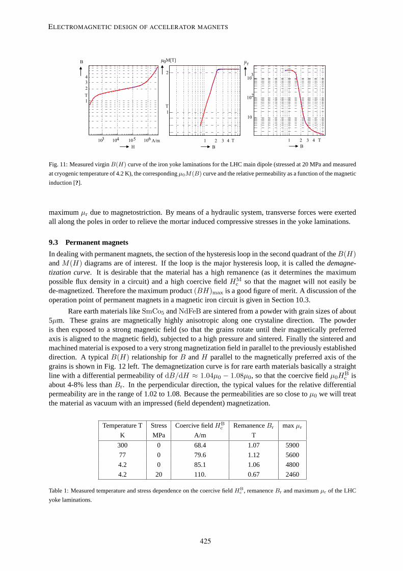
Fig. 11 shows the measured virginB(H) curve of the low carbon steel laminations used for theyoke of the LHC main dipoles, the correspondingM(B) curve and the relative permeability as a functionof the magnetic induction. The measurements were performed at 4.2 K with a ring specimen, a toroidalsuperconducting excitation coil and a copper search coil, in magnetic flux densities of up to 7.4 tesla.Table 1 gives the measured temperature and stress dependence on the coercive field, remanence andmaximum permeability of yoke laminations used in a LHC model magnet.

The properties of the magnetization curvesM(H) are governed by two mechanisms known asexchange couplingandanisotropy. Exchange coupling between electron orbitals in the crystal latticefavors long-range spin ordering over macroscopic distances and is isotropic in space. At temperaturesabove a critical value (for iron about 770oC) which is called the Curie temperature, the exchange cou-

1Thus the need to distinguish between the two coercive fieldsHBc andHM

c .

13


423

pling disappears. Anisotropy favors spin orientation along certain symmetry axes of the lattice. Thestudy of the quantum origin of these mechanisms is not needed in our phenomenological treatment ofthe material properties in field computation.

Many of the phenomena of the magnetization curve, i.e., the three sections between the “toe”, the“instep” and the “knee” can be described by means of the domain theory by Weiss, see for example [4].In an unmagnetized (and unstrained) piece of iron the directions in which the domains are magnetized areeither distributed at random (in parallel to one of the six crystal axes) or in such a way that the resultantmagnetization of the specimen is zero. Application of a magnetic field only changes the direction ofthe magnetization in a given volume and not the magnitude. This is attained by a reversible and laterirreversible boundary displacement of the domains. Saturation in high field is attained by a reversibleprocess of rotation within the domains.

9.2 Magnetostriction

A ferromagnetic specimen changes its dimensions by some parts per million when it is magnetized.This effect is referred to asmagnetostriction(positive for materials showing expansion and negative forcontraction). The effect is due to magneto-crystalline anisotropy which gives rise to energy variationswhen the relative positions of magnetic ions in the lattice are modified. It is usually distinguished betweenJoule magnetostriction (the change of dimension transversely to the field) and volume magnetostriction.In case of inverse magnetostriction or stress anisotropy, the deformation caused by an externally appliedstress favors certain magnetization directions.

Table 1 gives the measured temperature and stress dependence on the coercive field, remanenceand maximumµr of yoke laminations for a LHC model magnet. An aluminum ring around the ringspecimen provided for mechanical stress in the order of 20 MPa.

The main dipole magnets for LEP were built with a small packing factor of 0.27, realized byregularly spaced magnetic steel laminations and spaces filled with cement mortar. This solution providedfor mechanical rigidity at low price. Mortar shrinkage at hydration had an effect on the longitudinalmagnet geometry which was well controlled by means of four tie rods. In the transverse plane, however,the steel laminations opposed the shrinkage of the mortar layers so that tensile stresses built up in themortar (about 10 MPa, near the upper limit of mortar yield strength) and compressive stresses built up inthe iron laminations (at about 30 MPa due to a different elastic modulus and thickness of the layers). Thisresulted in an unacceptable∆B/B in the bending field at low excitation caused by the reduction of the

- 2 . 0

- 1 . 0

0 .

1 . 0

2 . 0

0 . 1 5 1 00 . 10 . 0 5 0- 0 . 0 5- 0 . 1- 0 . 1 5 1 0 0 5 0 0- 5 0- 1 0 0 - 1 . 5

- 1 . 0

- 0 . 5

0 .

0 . 5

1 . 0

1 . 5

2 1 0- 1- 2

F e N d B7 7 1 5 83 % S i - F e

- 3A / mT

T

T

T

µ0M

Hµ0H

T

µ0H

µ0M

Fig. 10: Left: M(B) hysteresis curve for soft (3%Si-Fe) grain oriented laminations used in transformer cores. Right:M(B)

hysteresis curve for a sinteredFe77Nd15B8 permanent magnet. Loop width differ by a factor of10−5. The low-carbon steel

used for the LHC yoke laminations is specified to have a coercive fieldHBc of less than 80±10 A/m at room temperature.

14

R. RUSSENSCHUCK

424

1234

1 2 3 4

1

2

1 2 3 41 0 1 0 1 0 1 03 4 5 6

1 0

1 0

1 0

2

3

HT

B

T

u M [ T ] u r0

T

A / mB B

T

Fig. 11: Measured virginB(H) curve of the iron yoke laminations for the LHC main dipole (stressed at 20 MPa and measured

at cryogenic temperature of 4.2 K), the correspondingµ0M(B) curve and the relative permeability as a function of the magnetic

induction [?].

maximumµr due to magnetostriction. By means of a hydraulic system, transverse forces were exertedall along the poles in order to relieve the mortar induced compressive stresses in the yoke laminations.

9.3 Permanent magnets

In dealing with permanent magnets, the section of the hysteresis loop in the second quadrant of theB(H)andM(H) diagrams are of interest. If the loop is the major hysteresis loop, it is called thedemagne-tization curve. It is desirable that the material has a high remanence (as it determines the maximumpossible flux density in a circuit) and a high coercive fieldHM

c so that the magnet will not easily bede-magnetized. Therefore the maximum product(BH)max is a good figure of merit. A discussion of theoperation point of permanent magnets in a magnetic iron circuit is given in Section 10.3.

Rare earth materials likeSmCo5 andNdFeB are sintered from a powder with grain sizes of about5µm. These grains are magnetically highly anisotropic along one crystaline direction. The powderis then exposed to a strong magnetic field (so that the grains rotate until their magnetically preferredaxis is aligned to the magnetic field), subjected to a high pressure and sintered. Finally the sintered andmachined material is exposed to a very strong magnetization field in parallel to the previously establisheddirection. A typicalB(H) relationship forB andH parallel to the magnetically preferred axis of thegrains is shown in Fig. 12 left. The demagnetization curve is for rare earth materials basically a straightline with a differential permeability ofdB/dH ≈ 1.04µ0 − 1.08µ0, so that the coercive fieldµ0H

Bc is

about 4-8% less thanBr. In the perpendicular direction, the typical values for the relative differentialpermeability are in the range of 1.02 to 1.08. Because the permeabilities are so close toµ0 we will treatthe material as vacuum with an impressed (field dependent) magnetization.

Temperature T Stress Coercive fieldHBc RemanenceBr maxµr

K MPa A/m T

300 0 68.4 1.07 5900

77 0 79.6 1.12 5600

4.2 0 85.1 1.06 4800

4.2 20 110. 0.67 2460

Table 1: Measured temperature and stress dependence on the coercive fieldHBc , remanenceBr and maximumµr of the LHC

yoke laminations.

15


425

00 . 2

0 . 4

0 . 6

0 . 8

1 . 0

1 . 21 . 4

00 . 20 . 40 . 60 . 81 . 01 . 21 . 4- 2 0 0 .- 4 0 0- 6 0 0- 8 0 0- 1 0 0 0 0

F e r r i t e

N e o d y m i u m I r o n B o r o n

A l N i C oS a m a r i u m C o b a l t

- 3

- 2

- 1

0

1

2

3

2 1 0 - 1 - 2 3 - 3 T

T T

k A / mT

BB

H−µ0H

B(H)

M(H)

µ0H

Fig. 12: Left: TypicalB(H) andM(H) curves for hard ferromagnetic substances (permanent magnets).M andH are both

pointing into the direction of the easy axis of the grains in the sinter material. Right: Demagnetization curves for different

permanent magnet materials at room temperature.

9.4 Magnetization currents and fictitious magnetic charges

In the presence of ferromagnets the magnetic field can be calculated as in vacuum, if all currents (includ-ing the magnetization currents) are explicitly considered

curlB = µ0(Jfree + Jmag) = µ0Jfree + µ0curlM(H). (68)

Hence

curl(

B− µ0M(H)µ0

)= Jfree. (69)

The magnetic inductionB is always source free but the magnetic fieldH is not:

div H = div(

B− µ0M(H)µ0

)= −div M(H) (70)

which gives rise to the definition of a fictitious magnetic charge of density

ρmag = −divµ0M(H) . (71)

A fictitious magneticsurfacecharge density, c.f. Fig. 13, is then defined as

σmag = µ0M(H) · dada

= µ0M(H) · n . (72)

+ + + + + + + + + + + +

- - - - - - - - - - - - M(H)BH

Fig. 13: Field, magnetic induction and magnetization in a permanent magnet.

16

R. RUSSENSCHUCK

426

This allows formally a treatment of magnetostatic problems in the same way as electrostatic problemsusing a magnetic scalar potential.

10 One-dimensional field calculation for conventional magnets

10.1 C-core dipole

Consider the magnetic circuit shown in Fig. 14 (left), a c-shaped iron yoke with two coils of all-togetherN turns around it. If the gap thickness is small compared to all other dimensions, the fringe field aroundthe gap will be small and we assume that the flux ofB through any cross section of the yoke (and acrossthe air-gap) will be constant. With Ampere’s law

∫∂a H · ds =

∫a J · da , we can write

Hi si +H0 s0 = Vm , (73)

1µ0µr

Bi si +1µ0B0 s0 = N I . (74)

With µr 1 we get the easy relation

B0 =µ0N I

s0. (75)

10.2 Quadrupole

For the quadrupole we can split up the integration path as shown in Fig. 14 right, from the origin to thepole (s1) along an arbitrary path through the iron yoke (s2) and back inside the aperture along the x-axis(s3). Neglecting the magnetic resistance of the yoke we get∮

H · ds =∫

s1

H1 · ds +∫

s3

H3 · ds = N I . (76)

As we will see later, in a quadrupole the field is defined by it’s gradientg with Bx = gy andBy = gx.Therefore the modulus of the field along the integration paths1 is

H =g

µ0

√x2 + y2 =

g

µ0r. (77)

Along thex-axis (s3) the field integral is zero becauseH ⊥ s. Therefore∫ r0

0Hdr =

g

µ0

∫ r0

0rdr =

g

µ0

r202

= N I, (78)

s 0n

T

1

2

3

r a

Fig. 14: Magnetic circuit of a conventional dipole magnet (left) a quadrupole magnet (right). Neglecting the magnetic resistance

of the iron yoke, an easy relation between the air gap field and the required excitational current can be derived.

17


427

w l

s 0a 0

a ms m

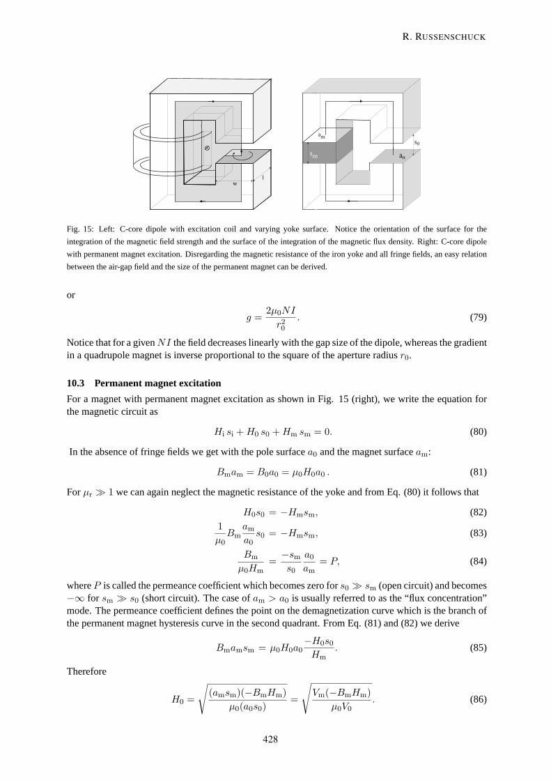
Fig. 15: Left: C-core dipole with excitation coil and varying yoke surface. Notice the orientation of the surface for the

integration of the magnetic field strength and the surface of the integration of the magnetic flux density. Right: C-core dipole

with permanent magnet excitation. Disregarding the magnetic resistance of the iron yoke and all fringe fields, an easy relation

between the air-gap field and the size of the permanent magnet can be derived.

or

g =2µ0NI

r20. (79)

Notice that for a givenNI the field decreases linearly with the gap size of the dipole, whereas the gradientin a quadrupole magnet is inverse proportional to the square of the aperture radiusr0.

10.3 Permanent magnet excitation

For a magnet with permanent magnet excitation as shown in Fig. 15 (right), we write the equation forthe magnetic circuit as

Hi si +H0 s0 +Hm sm = 0. (80)

In the absence of fringe fields we get with the pole surfacea0 and the magnet surfaceam:

Bmam = B0a0 = µ0H0a0 . (81)

Forµr 1 we can again neglect the magnetic resistance of the yoke and from Eq. (80) it follows that

H0s0 = −Hmsm, (82)1µ0Bm

am

a0s0 = −Hmsm, (83)

Bm

µ0Hm=−sms0

a0

am= P, (84)

whereP is called the permeance coefficient which becomes zero fors0 sm (open circuit) and becomes−∞ for sm s0 (short circuit). The case ofam > a0 is usually referred to as the “flux concentration”mode. The permeance coefficient defines the point on the demagnetization curve which is the branch ofthe permanent magnet hysteresis curve in the second quadrant. From Eq. (81) and (82) we derive

Bmamsm = µ0H0a0−H0s0Hm

. (85)

Therefore

H0 =

√(amsm)(−BmHm)

µ0(a0s0)=

√Vm(−BmHm)

µ0V0. (86)

18

R. RUSSENSCHUCK

428

S m C o

S m C o

5

5

Fig. 16: C-Core magnet with permanent magnet excitation. Top: With permanent magnet brought to the air gap in order to

reduce the fringe field. Display of vector potential and arrows representing the magnetic flux density are to scale.

For a given magnet volume, the maximum air gap field can be obtained by dimensioning the magneticcircuit in such a way thatBmHm is maximum.

Neglecting the leakage flux may be a rough treatment of the field problem, in particular for mag-netic flux densities exceeding 1 T in the yoke, or for large air gaps. Flux leakage is proportional to themagnetic potential difference, i.e., the m.m.f.Vm =

∫H · ds between the poles. The design shown

in Fig. 16 (bottom) is therefore a poor one, as there are large areas at high potential differences. Thestructure in Fig. 16 (top) with the permanent magnets brought to the air gap shows considerably lessleakage flux. For the use of permanent magnet material in accelerator magnets, demagnetization due toirradiation and thermal fluctuations has to be considered. As no permanent damage to the crystallinestructure of the magnet occurs, it is always possible to re-magnetize the magnet after irradiation to thenominal level.

11 Potential formulations for magnetostatic field problems

We will now show that in the aperture of a magnet (two-dimensional, current free region) both themagnetic scalar-potential as well as the vector-potential can be used to solve Maxwell’s equations:

H = −gradΦ = −∂Φ∂x

ex −∂Φ∂y

ey, (87)

B = curl(ezAz) =∂Az

∂yex −

∂Az

∂xey, (88)

and that both formulations yield the Laplace equation. These fields are called harmonic and the fieldquality can be expressed by the fundamental solutions of the Laplace equation. Lines of constant vector-potential give the direction of the magnetic field, whereas lines of constant scalar potential define theideal pole shapes of conventional magnets. Every vector field can be split into a source free and a curlfree part. In case of the magnetic field with

H = Hs + Hm, (89)

the curl free partHm arises from the induced magnetism in ferromagnetic materials and the source freepart Hs is the field generated by the prescribed sources (can be calculated directly by means of BiotSavart’s law). WithcurlHm = 0 it follows that

H = −gradΦm + Hs (90)

19


429

and we get:

div B = 0 , (91)

divµ(−gradΦm + Hs) = 0 , (92)

divµgradΦm = divµHs . (93)

While a solution of Eq. 93 is possible, the two parts of the magnetic fieldHm andHs tend to be of similarmagnitude (but opposite direction) in non-saturated magnetic materials, so that cancellation errors occurin the computation. For regions where the current density is zero, however,curlH = 0 and the field canbe represented by a total scalar potential

H = −gradΦ (94)

and therefore we get

−µ0 div gradΦ = 0 , (95)

∇2Φ = 0 , (96)

which is the Laplace equation for the scalar potential. The vector-operator Nabla is defined in Cartesiancoordinates as

∇ = (∂

∂x,∂

∂y,∂

∂z) (97)

and the Laplace operator

∆ = ∇2 =∂2

∂x2+

∂2

∂y2+

∂2

∂z2. (98)

The Laplace operator itself is essentially scalar. When it acts on a scalar function the result is a scalar,when it acts on a vector function, the result is a vector. Because ofdiv B = 0 a vector potentialA canbe introduced:B = curlA. We then get

curlA = µ0(H + M), (99)

H =1µ0

curlA−M, (100)

1µ0

curl curlA = J + curlM , (101)

1µ0

(−∇2A + grad divA) = J + curlM , (102)

Since the curl (rotation) of a gradient field is zero, the vector-potential is not unique. The gradientof any (differentiable) scalar fieldψ can be added without changing the curl ofA:

A0 = A + gradψ. (103)

Eq. (103) is called a gauge-transformation betweenA0 andA. B is gauge-invariant as the transformationfrom A to A0 does not changeB. The freedom given by the gauge-transformation can be used to set thedivergence ofA to zero

divA = 0, (104)

20

R. RUSSENSCHUCK

430

which (together with additional boundary conditions) makes the vector-potential unique. Eq. (104)is called the Coulomb gauge, as it leads to a Poisson type equation for the magnetic vector-potential.Therefore, from Eq. (102) we get after incorporating the Coulomb gauge:

∇2A = −µ0(J + curlM) . (105)

In the two-dimensional case with no dependence onz, ∂∂z = 0 andJ = Jz, A has only az-component

and the Coulomb gauge is automatically fulfilled. Then we get the scalar Poisson differential equation

∇2Az = −µ0Jz. (106)

For current-free regions (e.g. in the aperture of a magnet) Eq. (106) reduces to the Laplace equation,which reads in in cylindrical coordinates

r2∂2Az

∂r2+ r

∂Az

∂r+∂2Az

∂ϕ2= 0. (107)

11.1 Harmonic fields

A solution of the homogeneous differential equation (107) reads

Az(r, ϕ) =∞∑

n=1

(C1nrn + C2nr

−n)(D1n sinnϕ+D2n cosnϕ). (108)

Considering that the field is finite atr = 0, theC2n have to be zero for the vector-potential inside theaperture of the magnet while for the solution in the area outside the coil allC1n vanish. RearrangingEq. (108) yields the vector-potential in the aperture:

Az(r, ϕ) =∞∑

n=1

rn(Cn sinnϕ−Dn cosnϕ), (109)

and the field components can be expressed as

Br(r, ϕ) =1r

∂Az

∂ϕ=

∞∑n=1

nrn−1(Cn cosnϕ+Dn sinnϕ), (110)

Bϕ(r, ϕ) = −∂Az

∂r= −

∞∑n=1

nrn−1(Cn sinnϕ−Dn cosnϕ). (111)

Each value of the integern in the solution of the Laplace equation corresponds to a different flux distri-bution generated by different magnet geometries. The three lowest values, n=1,2, and 3 correspond to adipole, quadrupole and sextupole flux density distribution. The solution in Cartesian coordinates can beobtained from the simple transformations

Bx = Br cosϕ−Bϕ sinϕ, (112)

By = Br sinϕ+Bϕ cosϕ. (113)

For the dipole field (n=1) we get

Br = C1 cosϕ+D1 sinϕ, (114)

Bϕ = −C1 sinϕ+D1 cosϕ, (115)

Bx = C1, (116)

By = D1. (117)

21


431

This is a simple, constant field distribution according to the values ofC1 andD1. Notice that we have notyet addressed the conditions necessary to obtain such a field distribution. For the pure quadrupole (n=2)we get from Eq. (110) and (111):

Br = 2 r C2 cos 2ϕ+ 2 rD2 sin 2ϕ, (118)

Bϕ = −2 r C2 sin 2ϕ+ 2 rD2 cos 2ϕ, (119)

Bx = 2(C2x+D2y), (120)

By = 2(−C2y +D2x). (121)

The amplitudes of the horizontal and vertical components vary linearly with the displacements from theorigin, i.e., the gradient is constant. With a zero induction in the origin, the distribution provides linearfocusing of the particles. It is interesting to notice that the components of the magnetic fields are coupled,i.e., the distribution in both planes cannot be made independent of each other. Consequently a quadrupolefocusing in one plane will defocus in the other.

Repeating the exercise for the case of the pure sextupole (n=3) yields:

Br = 3 r C3 cos 3ϕ+ 3 rD3 sin 3ϕ, (122)

Bϕ = −3 r C3 sin 3ϕ+ 3 rD3 cos 3ϕ, (123)

Bx = 3C3(x2 − y2) + 6D3xy, (124)

By = −6C3xy + 3D3(x2 − y2). (125)

Along the x-axis (y=0) we then get the expression for the y-component of the field:

By = D1 + 2D2x+ 3D3x2 + 4D4x

3 + ... (126)

If only the two lowest order elements are used for steering the beam, forces on the particles are eitherconstant or vary linear with the distance from the origin. This is called a linear beam optic. It has tobe noted that the treatment of each harmonic separately is a mathematical abstraction. In practical situ-ations many harmonics will be present and many of the coefficientsCn andDn will be non-vanishing.A successful magnet design will, however, minimize the unwanted terms to small values. It has to bestressed that the coefficients are not known at this stage. They are defined through the (given) bound-ary conditions on some reference radius or can be calculated from the Fourier series expansion of the(numerically) calculated field, ref. Eq. (5), in the aperture using the relations

An = nrn−10 Cn and Bn = nrn−1

0 Dn. (127)

12 Ideal pole shapes of conventional magnets

Equipotentials are surfaces whereΦ is constant. For a pathds along the equipotential it therefore results

dΦ = gradΦ · ds = 0 (128)

i.e., the gradient is perpendicular to the equipotential. With the field lines (lines of constant vectorpotential) leaving highly permeable materials perpendicular to the surface (ref. Section 7), the lines oftotal magnetic scalar potential define the pole shapes of conventional magnets. As in 2D (with absenceof magnetization and free currents) the z-component of the vector potential and the magnetic scalarpotential both satisfy the Laplace equation, we already have the solution for a dipole field:

Φ = C1x+D1y. (129)

SoC1 = 0 , D1 6= 0 gives a vertical (normal) dipole field,C1 6= 0 , D1 = 0 yields a horizontal (skew)dipole field. The equipotential surfaces are parallel to the x-axis or y-axis depending on the values ofC

22

R. RUSSENSCHUCK

432

W i d t h

H e i g h t

x

y

y = c o n s t .

x

y

x y = c o n s t .

Fig. 17: Pole shape of a conventional dipole (right) and quadrupole magnet (left) with shims.

andD and results in a simple flux density distribution used for bending magnets in accelerators. For thequadrupole:

Φ = C2(x2 − y2) + 2D2xy (130)

with C2 = 0 giving a normal quadrupole field and withD2 = 0 giving a skew quadrupole field (which isthe above rotated byπ/4). The quadrupole field is generated by lines of equipotential having hyperbolicform. For theC2 = 0 case, the asymptotes are the two major axes.

In practice, however, the magnets have a finite pole width (due to the need of a magnetic flux returnyoke and space for the coil). To ensure a good field quality with these finite approximations of the idealshape, small shims are added at the outer ends of each pole. The shim geometry has to be optimizedusing numerical field computation tools. Fig. 17 shows the pole shape of a conventional dipole andquadrupole magnet, with magnetic shims.

Fig. 18 shows the cross-section of the LEP dipole and quadrupole magnets with iso-surfaces ofconstant vector-potential (for the dipole) and magnetic field modulus in the iron yoke for the quadrupole.The field quality in the dipole was improved by adding shims on the pole surface. In case of thequadrupole, however, the pole shape is defined as a combination of a hyperbola, a straight section andan arc. The points at which the segments are connected was found in an optimization process not onlyconsidering the multipole components in the cross-section, but also to provide for a part compensationof the end-effects.

13 Coil field of superconducting magnets

For coil dominated superconducting magnets with fields well above one tesla the current distribution inthe coils dominate the field quality and not the shape of the iron yoke. The problem therefore remainshow to calculate the field harmonics from a given current distribution. It is reasonable to focus on thefields generated by line-currents, since the field of any current distribution over an arbitrary cross-sectioncan be approximated by summing the fields of a number of line-currents distributed within the cross-section. For a set ofns of these line-currents at the position(ri,Θi) carrying a currentIi, the multipolecoefficients are given by [16]

Bn(r0) = −ns∑i=1

µ0Ii2π

rn−10

rni

(1 +

µr − 1µr + 1

(ri

Ryoke)2n

)cosnΘi, (131)

23


433

-0.13 0.864-

0.864 0.003-

0.003 0.005-

0.005 0.007-

0.007 0.009-

0.009 0.012-

0.012 0.014-

0.014 0.016-

0.016 0.018-

0.018 0.021-

0.021 0.023-

0.023 0.025-

0.025 0.028-

0.028 0.030-

0.030 0.032-

0.032 0.034-

0.034 0.037-

0.037 0.039-

0.039 0.041-

A (Tm)

0.664 0.110-

0.110 0.219-

0.219 0.328-

0.328 0.438-

0.438 0.547-

0.547 0.656-

0.656 0.766-

0.766 0.875-

0.875 0.984-

0.984 1.094-

1.094 1.203-

1.203 1.313-

1.313 1.422-

1.422 1.531-

1.531 1.641-

1.641 1.750-

1.750 1.859-

1.859 1.969-

1.969 2.078-

|Btot| (T)

Fig. 18: Cross-section of the LEP dipole and quadrupole magnets with iso-surfaces of constant vector-potential (left) and

magnetic field modulus (right).

An(r0) =ns∑i=1

µ0Ii2π

rn−10

rni

(1 +

µr − 1µr + 1

(ri

Ryoke)2n

)sinnΘi, (132)

whereRyoke is the inner radius of the iron yoke with the relative permeabilityµr. The field of any currentdistribution over an arbitrary cross-section can be approximated by summing the fields of a number ofline-currents distributed within the cross-section. As superconducting cables are composed of singlestrands with a diameter of about 1 mm, a good computational accuracy can be obtained by representingeach cable by two layers of equally spaced line-currents at the strand position. Thus the grading of thecurrent density in the cable due to the different compaction on its narrow and wide side is automaticallyconsidered.

With equations (131) and (132), a semi-analytical method for calculating the fields in supercon-ducting magnets is given. The iron yoke is represented by image currents (the second term in the paren-theses). At low field level, when the saturation of the iron yoke is low, this is a sufficient method foroptimizing the coil cross-section. Under that assumption some important conclusions can be drawn:

• For a coil without iron yoke the field errors scale with1/rn wheren is the order of the multipole

Fig. 19: Field vectors for a superconducting coil in a (non-saturated) iron yoke of cylindrical inner shape calculated by means

of the imaging current method.

24

R. RUSSENSCHUCK

434

andr is the mid radius of the coil. It is clear, however, that an increase of coil aperture causesa linear drop in dipole field. Other limitations of the coil size are the beam distance, the elec-tromagnetic forces, yoke size, and the stored energy which results in an increase of the hot-spottemperature during a quench.

• For certain symmetry conditions in the magnet, some of the multipole components vanish, i.e.for an up-down symmetry in a dipole magnet (positive currentI0 at (r0,Θ0) and at(r0,−Θ0))noAn terms occur. If there is an additional left-right symmetry, only the oddB1, B3, B5, B7, ..components remain.

• The relative contribution of the iron yoke to the total field (coil field plus iron magnetization) is fora non-saturated yoke (µr 1) approximately(1+(Ryoke

r )2n)−1. For the main dipoles with a meancoil radius ofr = 43.5 mm and a yoke radius ofRyoke = 89 mm we get for theB1 component a19% contribution from the yoke, whereas for theB5 component the influence of the yoke is only0.07%.

It is therefore appropriate to optimize for higher harmonics first using analytical field calculation, andinclude the effect of iron saturation on the lower-order multipoles only at a later stage.

14 The generation of pure multipole fields

Consider a current shellri < r < re with a current density varying with the azimuthal angleΘ, J(Θ) =J0 cosmΘ, then we get for theBn components

Bn(r0) =∫ re

ri

∫ 2π

0−µ0J0r

n−10

2πrn

(1 +

µr − 1µr + 1

(r

Ryoke)2n

)cosmΘcosnΘ rdΘdr . (133)

With∫ 2π0 cosmΘcosnΘdΘ = πδm,n(m,n 6= 0) it follows that the current shell produces a pure2m-

polar field and in the case of the dipole (m = n = 1) one gets

B1(r0) = −µ0J0

2

((re − ri) +

µr − 1µr + 1

1R2

yoke

13(r3e − r3i )

). (134)

Obviously, since∫ 2π0 cosmΘsinnΘdΘ = 0, allAn components vanish. A shell withcos Θ andcos 2Θ

dependent current density is displayed in Fig. 21. Because of|B| =∑

n

√B2

n +A2n the modulus of the

field inside the aperture of the shell dipole without iron yoke is given as

|B| = µ0J0

2(re − ri). (135)

14.1 Coil-block arrangements

Usually the coils do not consist of perfect cylindrical shells because the conductors itself are eitherrectangular or keystoned with an insufficient angle to allow for perfect sector geometries. Thereforethe shells are subdivided into coil-blocks, separated by copper wedges. The dipole coil consists of twolayers with cables of the same height but of different width. Both layers are connected in series so thatthe current density in the outer layer, being exposed to a lower magnetic field, is about 40% higher. Theconductor for the inner layer consists of 28 strands of 1.065 mm diameter, the outer layer conductorhas 36 strands of 0.825 mm diameter. The strands are made of thousands of filaments of NbTi materialembedded in a copper matrix which serves for stabilizing the conductor and to take over the current incase of a quench. The field generated by this coil layout is calculated with the line-current approximationof the superconducting cable. Real coil-geometries with one and two layers of coil-blocks are shown inFig. 21.

25


435

Fig. 20: Shells withcos Θ (left) andcos 2Θ (right) dependent current density.

Fig. 21: Coil-block arrangements made of Rutherford type cable. LHC main dipole model variant with two layers wound from

different cable.

15 Numerical field computation

Magnets for particle accelerators have always been a key application of numerical methods in electro-magnetism. Hornsby [12], in 1963, developed a code based on the finite difference method for the solvingof elliptic partial differential equations and applied it to the design of magnets. Winslow [22] created thecomputer code TRIM (Triangular Mesh) with a discretization scheme based on an irregular grid of planetriangles by using a generalized finite difference scheme. He also introduced a variational principle andshowed that the two approaches lead to the same result. In this respect, the work can be viewed as one ofthe earliest examples of the finite element method applied to the design of magnets. The POISSON codewhich was developed by Halbach and Holsinger [11] was the successor of this code and was still appliedfor the optimization of the superconducting magnets for the LHC during the early design stages. Halbachhad also, in 1967, [10] introduced a method for optimizing coil arrangements and pole shapes of magnetsbased on the TRIM code, an approach he named MIRT. In the early 1970’s a general purpose program(GFUN) for static fields had been developed by Newman, Turner and Trowbridge that was based on themagnetization integral equation and was applied to magnet design.

When the LHC magnets are ramped to their nominal field of 8.33 T, two nonlinear effects on themultipole field components appear: At low field due to the superconducting filament magnetization and

26

R. RUSSENSCHUCK

436

0 2 0 0 0 4 0 0 0 6 0 0 0 8 0 0 0 1 0 0 0 0 1 2 0 0 0 0 2 0 0 0 4 0 0 0 6 0 0 0 8 0 0 0 1 0 0 0 0 1 2 0 0 0

- 6

- 4

- 2

0

2

4

6

I IA A

b 2B / I

T / k A

0 . 7 0 3

0 . 7 0 4

0 . 7 0 5

0 . 7 0 7

0 . 7 0 8

0 . 7 0 9

0 . 7 1 0

0 . 7 0 6G e o m e t r i cP e r s i t e n t

S a t u r a t i o n

Fig. 22: Variation of the transfer functionB/I and the relative quadrupole field component as a function of the excitational

current. Note the effect of the iron saturation at higher field levels and the superconductor magnetization at low excitational

levels.

at high field due to the saturation of the iron yoke. Fig. 22 shows the transfer function and the quadrupolefield component in the main bending magnets as a function of the excitational current in these magnets.

For magnets with saturating iron yoke, numerical methods have to be used to replace the imagingmethod. It is advantageous to use numerical methods that do not require the modeling of the coils inthe finite-element mesh and allow a distinction between the coil-field and the iron magnetization effects,to confine both modeling problems on the coils and FEM-related numerical errors on the magnetizationeffects in the iron yoke. The integral equation method of GFUN would qualify but leads to a very large(fully populated) matrix of the linear equation system.

The disadvantage of the finite-element method is that only a finite domain can be discretized,and therefore the field calculation in the magnet coil-ends with their large fringe-fields requires a largenumber of elements in the air region. The relatively new boundary-element method is defined on aninfinite domain and can therefore solve open boundary problems without approximation with far-fieldboundaries. The disadvantage is that non-homogeneous materials are difficult to consider. The BEM-FEM method couples the finite-element method inside magnetic bodiesΩi = ΩFEM with the boundary-element method in the domain outside the magnetic materialΩa = ΩBEM, by means of the normalderivative of the vector-potential on the interfaceΓai between iron and air. The principle of the method isshown in Fig. 23. The application of the BEM-FEM method to magnet design has the following intrinsicadvantages:

• The coil field can be taken into account in terms of its source vector potentialAs, which can beobtained easily from the filamentary currentsIs by means of Biot-Savart type integrals without themeshing of the coil.

• The BEM-FEM coupling method allows for the direct computation of the reduced vector potentialAr instead of the total vector potentialA. Consequently, errors do not influence the dominatingcontributionAs due to the superconducting coil.

• Because the field in the aperture is calculated through the integration over all the BEM elements,local field errors in the iron yoke cancel out and the calculated multipole content is sufficientlyaccurate even for very sparse meshes.

• The surrounding air region need not be meshed at all. This simplifies the preprocessing and avoidsartificial boundary conditions at some far-field-boundaries. Moreover, the geometry of the perme-able parts can be modified without regard to the mesh in the surrounding air region, which strongly

27


437

y

IS

BS,i

Ω1

AΓ1AΓ2

BIRON

R1

BS,i

BIRON

R2

BS,i

Ω2

BEM-domain

FEM-domains

Ω3

Bi

CCCCCCCCCCC

Fig. 23: Elementary model problem for the BEM-FEM coupling method

supports the feature based, parametric geometry modeling that is required for mathematical opti-mization.

• The method can be applied to both 2D and 3D field problems.

15.1 LHC main dipole cross-section

The dipole magnet, its connections, and the bus-bars are enclosed in the stainless steel shrinking cylinderclosed at its ends and form the dipole cold-mass, a containment filled with static pressurized superfluidhelium at 1.9 K. The cold-mass, weighing about 24 tons, is assembled inside its cryostat, which com-prises a support system, cryogenic piping, radiation insulation, and thermal shield, all contained withina vacuum vessel.

Fig. 24 and 25 show the quadrilateral (higher order) finite element mesh of collar and yoke for theLHC main dipole, the magnetic field strength, the magnetic vector potential and the relative permeabilityin the iron yoke at nominal field level.

REFERENCES

[1] Armstrong, A.G.A.M. , Fan, M.W., Simkin, J., Trowbridge, C.W.: Automated optimization ofmagnet design using the boundary integral method, IEEE Transactions on Magnetics, 1982

[2] Bathe, K.-J: Finite Element Procedures, Prentice Hall, 1996[3] Bossavit, A.: Computational Electromagnetism, Academic Press, 1998[4] R.M. Bozorth: Ferromagnetism, IEEE Press Classic Reissue, 1993[5] Binns, K.J., Lawrenson, P.J., Trowbridge, C.W.: The analytical and numerical solution of electric

and magnetic fields, John Wiley & Sons, 1992[6] C.J. Collie: Magnetic fields and potentials of linearly varying current or magnetization in a plane

bounded region, Proc. of the 1st Compumag Conference on the Computation of ElectromagneticFields, Oxford, U.K., 1976

28

R. RUSSENSCHUCK

438

0.779 0.450-

0.450 0.899-

0.899 1.348-

1.348 1.797-

1.797 2.247-

2.247 2.696-

2.696 3.145-

3.145 3.595-

3.595 4.044-

4.044 4.493-

4.493 4.942-

4.942 5.392-

5.392 5.841-

5.841 6.290-

6.290 6.740-

6.740 7.189-

7.189 7.638-

7.638 8.087-

8.087 8.537-

|Btot| (T)

Fig. 24: Left: Quadrilateral (higher order) finite element mesh of collar and yoke for the LHC main dipole. Right: Magnetic

field strength in collar and yoke

-0.41 -0.37-

-0.37 -0.34-

-0.34 -0.31-

-0.31 -0.28-

-0.28 -0.24-

-0.24 -0.21-

-0.21 -0.18-

-0.18 -0.14-

-0.14 -0.11-

-0.11 -0.83-

-0.83 -0.50-

-0.50 -0.17-

-0.17 0.015-

0.015 0.048-

0.048 0.081-

0.081 0.113-

0.113 0.146-

0.146 0.179-

0.179 0.212-

A (Tm)

1.002 208.2-

208.2 415.5-

415.5 622.7-

622.7 830.0-

830.0 1037.-

1037. 1244.-

1244. 1451.-

1451. 1659.-

1659. 1866.-

1866. 2073.-

2073. 2280.-

2280. 2488.-

2488. 2695.-

2695. 2902.-

2902. 3109.-

3109. 3317.-

3317. 3524.-

3524. 3731.-

3731. 3938.-

MUEr

Fig. 25: Left: Magnetic vector potential; Right: Relative permeability in the iron yoke at nominal field level

[7] Biro, O., Preis, K., Paul. C.: The use of a reduced vector potential Ar Formulation for the calcula-tion of iron induced field errors, Proceedings of the First international ROXIE user’s meeting andworkshop, CERN, March 1998.

[8] Brebbia, C.A.: The boundary element method for engineers, Pentech Press, 1978.[9] Fetzer, J., Kurz, S., Lehner, G.: Comparison between different formulations for the solution of 3D

nonlinear magnetostatic problems using BEM-FEM coupling, IEEE Transactions on Magnetics,Vol. 32, 1996

[10] Halbach, K.: A Program for Inversion of System Analysis and its Application to the Design of Mag-nets, Proceedings of the International Conference on Magnet Technology (MT2), The RutherfordLaboratory, 1967

[11] Halbach, K., Holsinger R.: Poisson user manual, Techn. Report, Lawrence Berkeley Laboratory,Berkeley, 1972

[12] Hornsby, J.S.: A computer program for the solution of elliptic partial differential equations, Tech-nical Report 63-7, CERN, 1967

29


439

[13] Kurz, S., Fetzer, J., Rucker, W.M.: Coupled BEM-FEM methods for 3D field calculations withiron saturation, Proceedings of the First International ROXIE users meeting and workshop, CERN,March 16-18, 1998

[14] Kurz, S., Russenschuck, S.: The application of the BEM-FEM coupling method for the accuratecalculation of fields in superconducting magnets, Electrical Engineering, 1999

[15] S. Kurz and S. Russenschuck, The application of the BEM-FEM coupling method for the accuratecalculation of fields in superconducting magnets, Electrical Engineering, 1999.

[16] Mess, K.H., Schmuser, P., Wolff S.: Superconducting Accelerator Magnets, World Scientific, 1996[17] G.D. Nowottny, Netzerzeugung durch Gebietszerlegung und duale Graphenmethode, Shaker Ver-

lag, Aachen, 1999.[18] Russenschuck, S.: ROXIE: Routine for the Optimization of magnet X-sections, Inverse field cal-

culation and coil End design, Proceedings of the First International ROXIE users meeting andworkshop, CERN 99-01, ISBN 92-9083-140-5.

[19] Y. Saad, M.H. Schultz: GMRES: A Generalized Minimal Residual Algorithm For Solving Non-symmetric Linear Systems, SIAM Journal of Scientific Statistical Computing, 1986

[20] The LHC study group, Large Hadron Collider, The accelerator project, CERN/AC/93-03[21] The LHC study group, The Large Hadron Collider, Conceptual Design, CERN/AC/95-05[22] Winslow A.A.: Numerical solution of the quasi-linear Poisson equation in a non-uniform triangular

mesh, Jorunal of computational physics, 1, 1971[23] Wilson, M.N.: Superconducting Magnets, Oxford Science Publications, 1983[24] E.J.N. Wilson, Introduction to Particle Accelerators, 1996-1997[25] Wille, K.: Physik der Teilchenbeschleuniger und Synchrotronstahlungsquellen, Teubner, 1992

30

R. RUSSENSCHUCK

440

Documents

ELECTROMAGNETIC DESIGN OF ACCELERATOR MAGNETS · 2009-08-03 · ELECTROMAGNETIC DESIGN OF ACCELERATOR MAGNETS S. Russenschuck CERN, 1211 Geneva 23, Switzerland Abstract Analytical