Embed Size (px)
Citation preview

Proc. CERN Accelerator School on Measurement and Alignment of Accelerator andDetector Magnets, April 11-17, 1997, Anacapri, Italy, CERN-98-05, pp.1-26
BASIC THEORY OF MAGNETS
Animesh K. JainRHIC Project, Brookhaven National Laboratory, Upton, New York 11973-5000, USA
AbstractThe description of two dimensional magnetic fields of magnets usedin accelerators is discussed in terms of a harmonic expansion. Theexpansion is derived for cylindrical components and extended toCartesian components. The Cartesian components are also describedin terms of a complex field. The rules for transformation of theexpansion coefficients under various types of coordinate transfor-mation are given. The relationship between a given current distri-bution and the resulting field harmonics is explored in terms of thevector and complex potentials. Explicit results are presented for somesimple geometries. Finally, the harmonics allowed under varioussymmetries in the magnet current are discussed.
1. MULTIPOLE EXPANSION OF A TWO-DIMENSIONAL FIELD
For most practical purposes related to magnetic measurements in an accelerator magnet,one is interested in the magnetic field in the aperture of the magnet, which is in vacuum andcarries no current. Also, most accelerator magnets tend to be long compared to their aperture.Thus, a two dimensional description is valid for most of the magnet, except at the ends. Weshall at first confine ourselves to a description of a purely two dimensional field in a currentfree region. The relationship between the field and the currents will be treated later in Sec. 5and onwards.
In free space, with no true currents, the curl of the magnetic field, H, is zero. Also, themagnetic induction, B, is given by µ0H, where µ0 = 4π ×10-7 Henry/m is the permeability offree space. Consequently, the magnetic induction, B, can be expressed as the gradient of amagnetic scalar potential, Φm:
∇ × = ⇒ ∇ × = ⇒ = −∇ΦH B B0 0 m (1)
The magnetic induction, B = µ0H also has zero divergence. Combining this fact with Eq. (1),we get Laplace’s equation for the scalar potential:
∇ =2 0Φm (2)
We choose a cylindrical coordinate system with the Z-axis along the length of the magnet andthe origin located at the center of the magnet aperture. For a two dimensional field having noaxial component, the scalar potential has no z-dependence. Laplace’s equation can be solvedby separation of variables and imposing the boundary conditions that Φm be periodic in theangular coordinate, θ, and be finite at r = 0. The resulting general solution is a seriesexpansion of the scalar potential. The radial and the azimuthal components of B are then

2
obtained by taking the gradient of the scalar potential. The components of B in cylindricalcoordinates can be written in the form :
B rr
C nr
Rnr
m
refn
n
n( , ) ( ) sin[ ( )]θ∂
∂θ α= −
=
−
=
∞ −
∑Φ
1
1
(3)
B rr
C nr
Rnm
refn
n
nθ θ∂∂ θ
θ α( , ) ( ) cos[ ( )]= −
=
−
=
∞ −
∑1
1
1Φ
(4)
where C(n) and αn are constants and Rref is an arbitrary reference radius, typically chosen tobe 50-70% of the magnet aperture. For a given r, the n-th term in Br(r,θ ) has n maxima andn minima as a function of the azimuthal angle θ. These angular positions may be regarded asthe locations of magnetic poles. Thus, the n-th terms in Eqs. (3) and (4) correspond to a2n-pole field. Accordingly, C(n) is said to be the amplitude of the 2n-pole component of thetotal field. Τhe locations of the south and the north poles in the 2n-pole field are:
θπ
απ
απ
α= + + +2
52
92n n nn n n; ; ; .... SOUTH POLES (5)
θπ
απ
απ
α= + + +32
72
112n n nn n n; ; ; ....NORTH POLES (6)
The parameter αn defines the orientation of the 2n-pole component of the field withrespect to the chosen X-axis and is called the phase angle. Eqs. (3) and (4) represent themultipole expansion of the components of a two dimensional field in a current free region.
1.1 The Cartesian Components
Accelerator physicists often prefer to work with the Cartesian components of the field.The relationship between the Cartesian and the cylindrical components is shown in Fig. 1.
B
BrB
By
Bx
X-axis
Y-a
xis
θ
r
θ
θθ
Fig. 1 Cylindrical and Cartesian components of the magnetic induction vector, B

3
Using the expansions for Br and Bθ from Eqs. (3) and (4), we get the Cartesiancomponents:
B r B B C nr
Rn nx r
refn
n
n( , ) cos sin ( ) sin[( ) ]θ θ θ θ αθ= − =
− −
=
∞ −
∑1
1
1 (7)
B r B B C nr
Rn ny r
refn
n
n( , ) sin cos ( ) cos[( ) ]θ θ θ θ αθ= + =
− −
=
∞ −
∑1
1
1 (8)
1.2 The Complex Field
The components of a two dimensional field can be very conveniently described in termsof a complex field, B(z), defined as a function of the complex variable z = x + iy = r • exp(iθ )[a bold and italic font is used for complex quantities in this paper]. Looking at the expansionsin Eqs. (7) and (8), one could define the complex field as:
[ ]B zz
( ) ( , ) ( , ) ( )exp( )= + = −
=
∞ −
∑B x y iB x y C n inRy x n
n ref
n
α1
1
(9)
The divergence and the curl (in a source free region) of the vector B are zero. In twodimensions, we get:
∇ = ⇒
+
=
= −
. ,B 0 0
∂∂
∂
∂
∂
∂∂∂
Bx
B
y
B
yBx
x y y x or (10)
( ) ,∇ × = ⇒
−
=
=
B z
y x y xB
xBy
B
xBy
0 0∂
∂∂∂
∂
∂∂∂
or (11)
Eqs. (10) and (11) are nothing but the well known Cauchy-Riemann conditions for thecomplex field B(z) to be an analytic function of the complex variable z. The complex field issometimes defined as Bx(x, y) – iBy(x, y), which is also an analytic function of z. It should benoted that the quantity Bx + iBy is not an analytic function of z. The analytic property of thecomplex field has been exploited in solving many two dimensional problems [1-6].
2. TWO-DIMENSIONAL BEHAVIOUR OF THE INTEGRAL FIELD
In magnets of a finite length, the two dimensional representation of the field is validonly in the body of the magnet, sufficiently away from the ends. In regions near the ends ofthe magnet, the field is three dimensional and the usual multipole expansion is no longervalid. Some examples of a three dimensional treatment may be found in Refs. [7]-[9].However, for most practical purposes, one is interested in the integral of the field (or of itsderivatives) over the length of the magnet. This is because most magnets are short comparedto the wavelength of the betatron oscillations in the machine and the details of axial variationare of little consequence. Also, a typical rotating coil of a finite length only measures the

4
integral of the field over its length. It can be shown that the integral field behaves as a twodimensional field provided the integration is carried out over an appropriate region [10].
In general, for three dimensional fields in a current free region, the scalar potentialsatisfies the Laplace’s equation:
∇ = + +
=22
2
2
2
2
2 0ΦΦ Φ Φ
mm m mx y z
x y z( , , )
∂
∂
∂
∂
∂
∂(12)
Integrating along the Z-axis from Z1 to Z2, we get:
∫∂
∂
∂
∂
∂
∂∂
∂∂
∂
∂
∂
2
2
2
2
2
2
2
2
2
2
2
2
1
2
1
2
1
2
0Φ Φ Φ
ΦΦm m m
Z
Z
mZ
Zm
Z
Z
x y zdz
x yx y z dz
zdz+ +
⌠
⌡ = +
+⌠
⌡ =( , , ) (13)
We define the z-integrated scalar potential as ∫Φ Φm mZ
Zx y x y z dz( , ) ( , , )=
1
2. From Eq. (13):
∂
∂
∂
∂
∂∂
2
2
2
2 2 11
2Φ Φ Φm m m
Z
Z
z zx y z
B x y Z B x y Z+
= −
= −( , , ) ( , , ) (14)
If the region of integration is so chosen that the Z-component of the field is zero at theboundaries of this region, then the right hand side vanishes and the z-integrated scalarpotential satisfies the two dimensional Laplace’s equation. For example, the points Z1 and Z2
could both be chosen well outside the magnet on opposite ends to include the integral of thefield over the entire magnet. This situation is commonly encountered in the measurement ofthe integral field of relatively short magnets with a long integral coil. Alternatively, one couldchoose Z1 well outside the magnet and Z2 well inside the magnet, where the field is again twodimensional. Such a situation would apply to the measurement of the end region in a longmagnet with a short measuring coil. The measuring coil for this purpose must have sufficientlength so that the condition in Eq. (14) can be satisfied.
NORMAL AND SKEW COMPONENTS
The multipole expansion of the complex field is given by Eq. (9). The normal and skewcomponents are defined as the real and the imaginary parts of the expansion coefficients:
C(n)exp(–inαn) = (2n-pole NORMAL Term) + i(2n-pole SKEW Term) (15)
Unfortunately, the index n in the expansion coefficient is not the same as the correspondingpower (n–1) of z in Eq. (9). This has led to two different conventions being followed indenoting the normal and the skew terms. The “US Convention” denotes the 2n-pole normaland skew terms with an index of (n–1), to match the corresponding power of z in Eq. (9):
2 - pole Normal Term = 2 - pole Skew Term =
n C n n Bn C n n A
n n
n n
( )cos( )( )sin( )
αα
≡− ≡
−
−
1
1 “U.S. CONVENTION” (16)

5
On the other hand, the “European Convention” denotes the 2n-pole normal and skewcomponents with an index of n to retain the simple relationship between the index and thenumber of poles:
2 - pole Normal Term = 2 - pole Skew Term =
n C n n Bn C n n A
n n
n n
( )cos( )( )sin( )
αα
≡− ≡
“EUROPEAN CONVENTION” (17)
Even though the two conventions are commonly referred to as the “US” and the“European” notations, their use is not necessarily restricted to the respective geographicregions. This calls for exercising caution in interpreting the notations. One possible indicatorof the notation is the presence or the absence of B0 and A0 terms.
In terms of the normal and the skew components, the expansion of B(z) is:
[ ]B zz
( ) = + = +
=
∞
∑B iB B iARy x n n
n ref
n
0 “U.S. CONVENTION” (18)
[ ]B zz
( ) = + = +
=
∞ −
∑B iB B iARy x n n
n ref
n
1
1
“EUROPEAN CONVENTION” (19)
The corresponding equations for the radial and the azimuthal components of the fieldare:
[ ]B rr
RB n A nr
refn
n
n n( , ) sin{( ) } cos{( ) }θ θ θ=
+ + +
=
∞
∑0
1 1 “U.S. Convention” (20)
[ ]B rr
RB n A n
refn
n
n nθ θ θ θ( , ) cos{( ) } sin{( ) }=
+ − +
=
∞
∑0
1 1 “U.S. Convention” (21)
[ ]B rr
RB n A nr
refn
n
n n( , ) sin( ) cos( )θ θ θ=
+
=
∞ −
∑1
1
“European Convention” (22)
[ ]B rr
RB n A n
refn
n
n nθ θ θ θ( , ) cos( ) sin( )=
−
=
∞ −
∑1
1
“European Convention” (23)
It should be noted that sometimes the skew component is defined with a sign opposite tothat used here [11]. In view of the different notations in existence, it is important to recognizethe convention being used in any particular work.
It is possible to assign a physical significance to the normal and the skew components interms of the derivatives of the field. Using Eq. (18) or Eq. (19), it is easy to show that

6
B BR
n
B
x
A AR
nB
x
n nrefn n
yn
x y
n nrefn n
xn
x y
( ) ( )!
( ) ( )!
;
;
US European
US European
= =
= =
+
= =
+
= =
1
0 0
1
0 0
∂
∂
∂
∂
n ≥ 0 (24)
A magnet with the 2m-pole term as the most dominant term is called a normal magnet ifthe 2m-pole skew term is zero. Similarly, such a magnet is called a skew magnet if the normalterm is zero. As per Eqs. (16) and (17), the possible values of the phase angle for the 2m-poleterm are αm = 0 or π /m for a normal magnet and αm = π /(2m) or 3π /(2m) for a skew magnet.The poles in a 2m-pole magnet [see Eqs. (5) and (6)] are located at θ = π /(2m), 3π /(2m),5π /(2m), etc. for a normal magnet and at θ = 0, π /m, 2π /m, 3π /m, etc. for a skew magnet. A2m-pole skew magnet is obtained from a 2m-pole normal magnet by a clockwise rotation ofthe magnet by an angle π /(2m).
3.1 Fractional Field Coefficients, or “Multipoles”
The expansion coefficients Bn and An in Eqs. (18)-(23) are related to the actual fieldstrength in the magnet and are dependent on the excitation level. In describing the fieldquality of a magnet, one is often interested in the shape of the field, rather than its absolutemagnitude. This is done by expressing the various harmonic terms in the expansion as afraction of a reference field, Bref . For example, the complex field may be written as:
B zz
( ) ( , ) ( , )( )exp( )
= + =−
=
∞ −
∑B x y iB x y BC n in
B Ry x refn
refn ref
nα
1
1
(25)
Generally, this reference field is chosen as the strength of the most dominant term in theexpansion. For a 2m-pole magnet, it is expected that the term for n = m will be the mostdominant one. Hence, Bref may be chosen to be equal to C(m). Sometimes the reference fieldis chosen as the strength of the dipole field used for bending the beam in a circularaccelerator.
The Normal and Skew 2n-pole fractional field coefficients, or “multipoles” are definedas:
bC n in
BBB
aC n in
BABn
n
ref
n
refn
n
ref
n
ref−
−−
−=−
= =−
=11
11Re
( )exp( ), Im
( )exp( )α α (US) (26)
bC n in
BB
Ba
C n inB
ABn
n
ref
n
refn
n
ref
n
ref=
−
= =−
=Re( )exp( )
, Im( )exp( )α α
(European) (27)
In a typical accelerator magnet, the multipoles are of the order of 10-4 when calculatedat a reference radius comparable to the size of the region occupied by the beam (~ 50-70% ofthe coil radius). The coefficients are therefore often quoted after multiplying by a factor of104. With this multiplicative factor, the values of the multipoles are said to be in “ units”.

7
3. TRANSFORMATION OF FIELD PARAMETERS
The expansion parameters [C(n), αn] or [Bn, An] depend on the choice of the referenceframe. For example, the parameter αn controls the angular locations of the poles for the2n-pole component of the field according to Eqs. (5) and (6). If the coordinate axes (orequivalently, the magnet) are rotated, the angular positions of the poles would change, thusnecessitating a corresponding change in the parameter αn. In general, the quantities Bn and An
should be regarded as expansion coefficients according to Eq. (18) or (19), which clearlydepend on the choice of coordinate axes, since the variable z depends on the coordinate axesused. In this section, we shall derive the equations that govern the transformation of theseparameters under commonly encountered coordinate transformations.
4.1 Displacement of Axes
Let us consider a frame X’-Y’which is displaced from a frame X-Y by z0 = x0 + iy0 asshown in Fig. 2. The axes in the two frames are assumed to be parallel. In other words, thereis no rotation of the axes. The field parameters are denoted by [C(n), αn] or [Bn, An] in the X-Yframe and by [ ]′ ′C n n( ),α or [ , ]′ ′B An n in the X’-Y’frame.
We consider a point, P, in space located at z = x + iy in the X-Y frame. The same point islocated at z’ = x’ + iy’ = z – z0 in the X’-Y’ frame, as shown in Fig. 2. Since the coordinateaxes in the two frames are parallel to each other, the Cartesian components of the field are thesame in the two frames. In other words, the complex field is the same in the two frames. Thisfact can be used to derive the expansion of the field in the X’-Y’ frame as follows:
B z B z
z z + z
z z
( ) ( )
( ) ( )
( )!
!( )!
′ = + = + =
= +
= +
′
= +−
′
′ ′
=
∞
=
∞
=
∞
=
−
∑ ∑
∑ ∑
B iB B iB
B iAR
B iAR
B iAk
n k n R R
y x y x
kk
kref
k
kk
kref
k
kk
kn
k
ref
n
ref
k n
0 0
0
0 0
0
(28)
X
Y
X '
Y '
O
O'
r 0
x0
y0ξ
z = x + iy=(x'+x0) + i (y'+y0)
z' = x' + iy'x'
x
y'y
z0 = x0+ iy0
= r0. exp (i ξ)
P
Fig. 2 Displacement of coordinate axes

8
In writing the above equations, we have used the US convention as per Eq. (18). With arearrangement of terms in the double summation, it can be shown that
n
k
knk k n
knn
t t==
∞
=
∞
=
∞
∑∑ ∑∑=00 0
(29)
Applying this identity to Eq. (28), we may write:
B zz z z
( ) ( )!
!( )!( )′ = +
−
′
= ′ + ′
′
=
∞ −
=
∞
=
∞
∑∑ ∑B iAk
n k n R RB iA
Rk kk n ref
k n
n ref
n
nn n
ref
n0
0 0
(30)
The expansion coefficients in the displaced frame are therefore given by:
( ) ( )!
!( )!′ + ′ = +
−
+
≥
=
∞ −
∑B iA B iAk
n k nx iy
Rnn n k
k nk
ref
k n0 0 0 ; (US Notation) (31)
The corresponding equation in the European notation is:
( ) ( )( )!
( )!( )!′ + ′ = +
−− −
+
≥
=
∞ −
∑B iA B iAk
n k nx iy
Rnn n k
k nk
ref
k n1
110 0 ; (European Notation)(32)
The transformation for the amplitude and phase of the 2n-pole term is given by:
C n in C k ikk
n k nx iy
Rnn k
k n ref
k n
′ − ′ = −−
− −
+
≥
=
∞ −
∑ ; ( )exp( ) [ ( )exp( )]( )!
( )!( )!α α
11
10 0 (33)
It is seen from Eqs. (31)-(33) that coefficients of any particular order in the displacedframe are given by a combination of all the terms of equal or higher order in the undisplacedframe. Conversely, a given harmonic term in the undisplaced frame contributes to all theharmonics of equal or lower order in the displaced frame. For example, a displacement in apure quadrupole magnet will result in a dipole term in addition to the quadrupole term, adisplacement in a pure sextupole field will produce quadrupole and dipole fields and so on.This effect is referred to as the feed down of harmonics. Eq. (33) is useful in estimating theeffect of magnet misalignment in an accelerator, or in calculating the location of measuringcoil in the magnet during measurements.
4.2 Rotation of Axes
Let us consider a frame X’-Y’which is rotated with respect to a frame X-Y by an angleφ as shown in Fig. 3. The origins of the two frames are the same. The field parameters aredenoted by [C(n), αn] or [Bn, An] in the X-Y frame and by [ ]′ ′C n n( ),α or [ , ]′ ′B An n in theX’-Y’frame. The relationship between the two sets of expansion coefficients can be obtainedby using the relationship between the complex coordinates z and z’ and the relationshipbetween the Cartesian components in the two frames, as was done for the case of adisplacement of axes in Sec. 4.1. For the case of a rotation by an angle φ, we have

9
B B Bx x y′ = +cos sinφ φ ; B B By x y′ = − +sin cosφ φ (34)
z z= ′ exp( )iφ (35)
Following the US convention, we may write
B zz
z z
( ) ( )exp( ) [ ] exp( )
[ ] exp[ ( ) ] [ ]
′ = + = + = +
= +′
+ = ′ + ′
′
′ ′=
∞
=
∞
=
∞
∑
∑ ∑
B iB B iB i B iAR
i
B iAR
i n B iAR
y x y x nn
nref
n
nn
nref
n
nn
nref
n
φ φ
φ
0
0 01
(36)
The transformation of coefficients follows immediately from the above equation:
( ) ( )exp[ ( ) ]′ + ′ = + + ≥B iA B iA i n nn n n n 1 0φ ; (US Notation) (37)
( ) ( )exp( )′ + ′ = + ≥B iA B iA in nn n n n φ ; 1 (European Notation) (38)
The transformation for the amplitude and phase of the 2n-pole term is given by:
′ − ′ = −C n in C n in inn n( )exp( ) ( )exp( )exp( )α α φ ⇒ ′ = ′ = − ≥C n C n nn n( ) ( ); ; α α φ 1 (39)
As seen from Eqs. (37)-(39), a rotation of axes does not produce any feed down ofharmonics, but causes mixing of the normal and the skew components of a given harmonic.
4.3 Reflection of X-Axis: Magnet Viewed from the Opposite End
If a magnet is viewed from the end which is opposite to the end from which the fieldparameters are measured, then appropriate transformation must be applied to the fieldparameters. Such a situation may be encountered in practice when all magnets in an
X
Y
X '
Y '
φ
B
Bx
By
Bx'By'
r
θ
z = z' exp(iφ)
Fig. 3 Rotation of axes

10
accelerator are measured from the same end, but all magnets are not installed with the leadsfacing the same way. The reference frames X-Y and X’-Y’ are shown in Fig. 4. The Y’-axiscoincides with the Y-axis but the X’-axis points away from the X-axis.
To obtain the transformation, we note that
z z* = − = − ′ − ′ = − ′x iy x iy (40)
B iB B iB B iB B iAR
B iAR
B iAR
y x y x y x nn
nref
n
nn
nn
ref
n
nn
nref
n
′ ′=
∞
=
∞
=
∞
+ = − = + = +
= − −′
= ′ + ′
′
∑
∑ ∑
( )* ( )**
( )( ) ( )
0
0 0
1
z
z z(41)
From Eq. (41), it immediately follows that
′ = − ′ = − ≥+B B A A nnn
n nn
n( ) ( )1 1 01 ; ; (US Notation) (42)
′ = − ′ = − ≥+B B A A nnn
n nn
n( ) ( )1 1 11 ; ; (European Notation) (43)
′ = ′ = − ′ =
− ≥− −C k C kk
kk k k k( ) ( ); ; ; α α απ
α2 1 2 1 2 221 (44)
It should be noted that the transformations given in Eqs. (42) and (43) are for theunnormalized normal and skew coefficients. In practice, one often deals with the normalizedfractional field coefficients, or multipoles, defined in Sec.3.1. The transformation of themultipoles can be a source of considerable confusion depending on how the reference field ischosen. For example, in a normal quadrupole magnet, the main field component (the normalquadrupole term) will change sign when viewed from the opposite end according to Eq. (42)
XX '
Y, Y '
O,O '
B
Bx = –Bx'
B y = B
y'
z* = –z'
Fig. 4 Reflection of X-Axis: magnet viewed from the opposite end

11
or Eq. (43). However, one may like to normalize the multipoles in such a way that the mainmultipole, b1 (or b2 in the European notation) is always positive. With such a normalization,the normal quadrupole multipole in this case will not change sign under a reflection of axes.Therefore, while deriving the transformation rules for the normalized multipoles, one shouldalso pay attention to the normalization rules. The principal use of the measured multipoles isto provide a series expansion of the field for use in accelerator physics studies. Thetransformation rules for the multipoles must be derived in such a way that the form of theexpansion used in such studies remains valid.
4. RELATIONSHIP BETWEEN CURRENT AND MAGNETIC FIELD
The harmonic expansion of the components of the magnetic induction, B, derived inSec.1 made no reference to the current distribution that produced the field. In practice, thedistribution of current in an electromagnet determines the shape of the field, and hence theactual values of the normal and skew components, or the amplitudes and phases of variousharmonics. From the point of view of magnet design as well as magnetic measurements, it isessential to have an understanding of the relationship between current distribution in a magnetand the field harmonics.
In order to study the relationship between current and the field shape, it is convenient todescribe the magnetic induction B in terms of the vector potential, A. From Maxwell’sequations, the divergence of B is zero everywhere. So, we may write
B A= ∇ × (ALWAYS HOLDS) (45)
If we restrict ourselves to regions where B = µ0H, then we also have
∇ × = ∇ × ∇ × = ∇ ∇ − ∇ = ∇ × =B A A A H J( ) ( . ) ( )20 0µ µ (46)
where J is the current density vector. Since only the curl of A is important, we may add anarbitrary term ∇ψ to A without affecting the results (Gauge Transformation). We choose thisterm ∇ψ in such a way that the divergence of A becomes zero. With this choice of gauge, weget the Poisson’s equation for the vector potential,
∇ = −20A Jµ (47)
The solution of the Poisson’s equation is given by [12]
A rJ(r )r r
r( )| |
=
′− ′
⌠⌡
′µπ0
4 d (48)
If the distribution of current is known, one can obtain the vector potential, and hence themagnetic induction, B. In the presence of magnetic materials, the current density in Eq. (48)must also include the current loops that effectively produce the magnetization. Thiscomplicates the application of Eq. (48) in practice. We shall derive expressions for themagnetic induction for several simple geometries of interest in Sec. 7.
12
6. THE COMPLEX POTENTIAL
The scalar and the vector potentials can be combined into a single complex potential.For a two dimensional field confined to the X-Y plane, the current and the vector potentialhave only a Z-component. Let us define a function, W(z), as a function of the complexvariable z by the relation
W z( ) ( , ) ( , )= +A x y i x yz mΦ (49)
where Az is Z-component of the vector potential and Φm is the magnetic scalar potential.Then,
−
≡ −
= −
−
= + =
dd x
Ax
ix
B x y iB x yz my x
W zz
W zB z
( ) ( )( , ) ( , ) ( )
∂∂
∂∂
∂∂Φ
(50)
The derivative of W(z) in the complex plane is the complex field B(z) defined in Eq. (9).We may think of W(z) as a complex potential. It should be noted that slightly differentversions of the complex potential exist in the literature depending on the definition of thecomplex field. The complex potential for simple current geometries can be easily calculated,leading to several useful results, as we shall see in the next section. The complex potentialinvolves both the vector and the scalar potential, and, therefore, contains more informationthan is necessary to describe the field. However, it has the advantage of being an analyticfunction of the complex variable, z.
7. FIELD DUE TO SOME SIMPLE CURRENT DISTRIBUTIONS
In this section we shall derive the expressions for the field from some very simple typesof current distributions. Since we are dealing with only two dimensional fields, all the currentdistributions will be assumed to have an infinite extent in the Z-direction.
7.1 An Infinitesimally Thin Current Filament
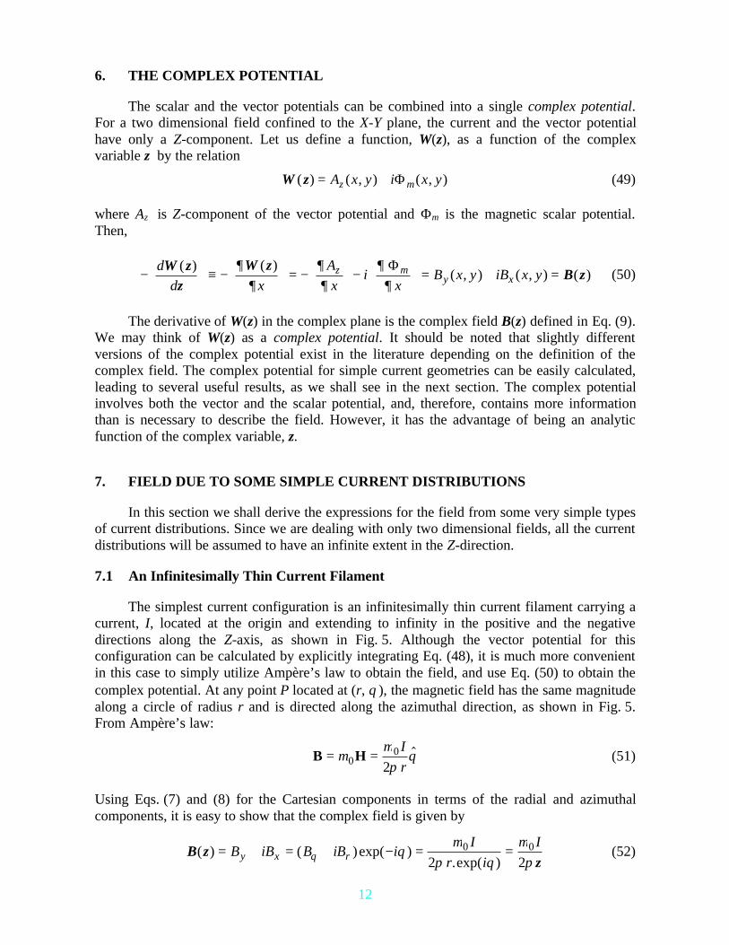
The simplest current configuration is an infinitesimally thin current filament carrying acurrent, I, located at the origin and extending to infinity in the positive and the negativedirections along the Z-axis, as shown in Fig. 5. Although the vector potential for thisconfiguration can be calculated by explicitly integrating Eq. (48), it is much more convenientin this case to simply utilize Ampère’s law to obtain the field, and use Eq. (50) to obtain thecomplex potential. At any point P located at (r, θ ), the magnetic field has the same magnitudealong a circle of radius r and is directed along the azimuthal direction, as shown in Fig. 5.From Ampère’s law:
B H= =µµπ
θ00
2Ir
$ (51)
Using Eqs. (7) and (8) for the Cartesian components in terms of the radial and azimuthalcomponents, it is easy to show that the complex field is given by
B zz
( ) ( )exp( ).exp( )
= + = + − = =B iB B iB iI
r iI
y x rθ θµ
π θµπ
0 0
2 2(52)
13
The complex potential is obtained by integrating the complex field:
W z z z z( ) ( ) ln( ) [ln( ) ]= − = −
+ = −
+ +∫ B dI I
r iµ
πµ
πθ0 0
2 2constant constant (53)
The real and the imaginary parts of W(z) give the vector potential, Az, and the scalar potential,Φm, respectively [see Eq. (49)].
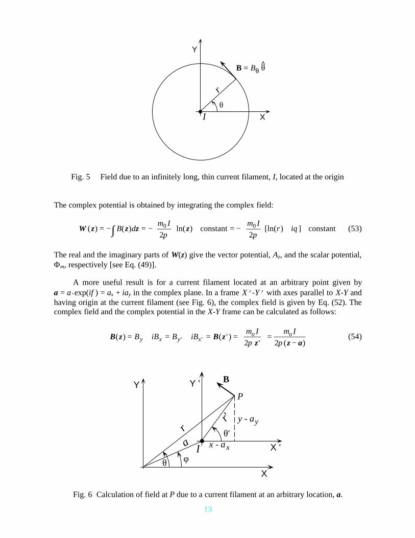
A more useful result is for a current filament located at an arbitrary point given bya = a • exp(iφ) = ax + iay in the complex plane. In a frame X’-Y’ with axes parallel to X-Y andhaving origin at the current filament (see Fig. 6), the complex field is given by Eq. (52). Thecomplex field and the complex potential in the X-Y frame can be calculated as follows:
B z B zz z a
( ) ( )( )
= + = + = ′ =′
=
−′ ′B iB B iBI I
y x y xo oµ
πµ
π2 2(54)
rθ
X
Y
I
B = Bθ θ ^
Fig. 5 Field due to an infinitely long, thin current filament, I, located at the origin
r'θ'
X '
Y '
I
B
P
r
θ φ
a
X
Y
x - ax
y - ay
Fig. 6 Calculation of field at P due to a current filament at an arbitrary location, a.

14
W z B z z z a( ) ( ) ln( ) [ln( ) ]= − = −
− + = −
′ + ′ +∫ dI I
r iµ
πµ
πθ0 0
2 2const. const. (55)
Using Eq. (54), we can determine, in principle, the field due to any arbitrary distributionof current by treating it as a superposition of current filaments. We shall see some simpleexamples in the rest of this section.
7.2 Cylindrical Current Sheet of Uniform Density
Let us calculate the complex field due to an infinitely long, infinitesimally thincylindrical conductor of radius a carrying a current I, as shown in Fig. 7. The current densityis assumed to be uniform. Also, all currents are assumed to flow parallel to the length of thecylinder, which is along the Z-axis. The complex field at z from a small element of angularwidth dφ, located at angle φ and carrying a current dI, can be calculated using Eq. (54). Thetotal field can then be obtained by integrating over the entire surface of the cylinder:
B zz z
zz z z
( )exp( ) exp( ) ( )
=
−⌠⌡
=
−
⌠⌡
=
′′ − ′
⌠⌡
µπ φ
µπ π
φφ
µπ π
π
0 0
0
2
0
2 2 2 21
2dI
a iI d
a iI
id
(56)
where we have used the transformation z’= a.exp(iφ) and the contour integral is along thesurface of the cylinder. The integrand in Eq. (56) has two simple poles, at z’= 0 and z’= z. Ifthe field point z is outside the cylinder, then only the pole at z’= 0 contributes to the integral.Similarly, if the field point z is inside the cylinder, both the poles contribute to the integral.Using the method of residues, it is easy to show that the total complex field in the regionsoutside and inside the cylinder is given by
B zz
B zout inI
( ) ; ( )=
=
µπ0
20 (57)
Thus, the field inside the cylinder is zero, while for any point outside, the cylinderbehaves as an infinitesimally thin current filament located at the center.
a
φX
Y
Idφ
dI
Bin(z) Bout(z)
Fig. 7 A section of a thin, cylindrical sheet carrying current I along the Z-axis.

15
7.3 Solid Cylindrical Conductor with Uniform Current Density
We now consider an infinitely long solid cylinder of radius a carrying a total current Ialong the Z-axis, as shown in Fig. 8. The field at any point can be obtained by dividing thesolid cylinder into thin cylindrical shells and using the results of Sec.7.2. For any pointoutside the cylindrical conductor, all such shells contribute. For any point P at a radius r < a,as shown in Fig. 8, only shells with radii ξ < r contribute.
The current density J is given by I /(π a2). The current carried by a thin shell of radius ξand thickness dξ is given by dI = J.2πξ.dξ. For any point inside the cylinder, the totalcomplex field is:
B zz z z
zino o
ro odI J
dJr J
( ) . . *=
⌠⌡
=
⌠⌡
=
=
µπ
µξ ξ
µ µ2 2 2
0
2(58)
where we have used the fact that r2 =zz*. For any point outside the solid cylinder, the totalcomplex field is:
B zz z z zout
o oa
o odI Jd
Ja J a( ) . .=
⌠⌡
=
⌠⌡
=
=
µπ
µξ ξ
µ µ2 2 2
0
2 2(59)
It should be noted that Bin(z) is a function of z*, and hence is not an analytic function ofz. This result is not unexpected, because the points inside the cylinder are not in a source freeregion. The analyticity of the complex field defined as By + iBx was shown in Sec.2 to followfrom Maxwell’s equations in a current free region only [see Eq. (11)].
a
ξ
dξ
rdI
X
Y
I
PBin(z)
Bout(z)
Fig. 8 Calculation of field due to a solid cylindrical conductor.

16
7.4 Solid Conductor of Arbitrary Cross Section
Let us now consider a solid conductor of arbitrary cross section defined by the contourC in the complex plane, as shown in Fig. 9. In principle, one could calculate the field fromsuch a conductor by integrating the result for a thin current filament [see Eq. (54)] over thecross section of the conductor. This approach requires a two dimensional integral to beevaluated and is not always convenient. A much simplified result has been obtained byBeth[2] by defining a complex function which is analytic everywhere, including the region ofthe conductor, and then evaluating the field as a contour integral around the path C. The resultof Beth, referred to as the integral formula, is briefly summarized here.
Inside the region of the conductor, Maxwell’s equations give:
( ) ( , );∇ × =
−
= ∇ ⋅ =
+
=B Bz
y xz
x yB
xBy
J x yBx
B
y
∂
∂∂∂
µ∂∂
∂
∂0 0 (60)
where Jz (x, y) is the current density at the point (x, y). For a constant current density over thecross section of the conductor, Jz(x,y) = J, it can be easily shown that the function:
F z z B z z( ) ( , ) ( , ) * ( ) *= + −
= −
B x y iB x yJ J
y xµ µ0 0
2 2(61)
satisfies Cauchy-Riemann conditions and is, therefore, an analytic function of the complexvariable, z. For points outside the conductor, J = 0, and F(z) becomes identical to B(z). It hasbeen shown by Beth [2] that this function, F(z), can be evaluated as a contour integral overthe boundary of the conductor. The complex field is then calculated using Eq. (61). The finalresult is given by:
B z F z z*z
z zz z* z = zin
C
inJ
iJ
dJ
( ) ( )*
;= +
=
′′ −
⌠⌡
′ +
µ µπ
µ0 0 0
2 4 2 for (62)
X
Y
z'
zout
zin Bin Bout
C
J
Fig. 9 Section of an infinitely long solid conductor of arbitrary cross section.

17
B z F zz
z zz z = zout
C
outiJ
d( ) ( )*
,= =
′′ −
⌠⌡
′µ
π0
4 for (63)
The expressions for the field are thus reduced to an integral along the perimeter of theconductor cross section, rather than a two dimensional integral over the area of the conductorcross section. It should be noted that the integrand in Eqs. (62) and (63) contains z’*, and isnot an analytic function of the complex variable. The method of residues is not applicable ingeneral and the integral must be explicitly evaluated.
A quick verification of the integral formula can be made for the case of a solid circularcylinder, for which the expression for field was derived in Sec.7.3. For this special case,z’* = a.exp(–iφ) = a2/ z’, which is an analytical function with a simple pole at z’= 0. Theintegral in Eqs. (62) and (63) becomes identical to the one in Eq. (56) evaluated earlier inSec.7.2. Using the results of Sec.7.2, it is easy to verify that Eqs. (62) and (63) give the sameresults for a solid cylindrical conductor as Eqs. (58) and (59).
7.5 Application of the Integral Formula: A Solid Elliptical Conductor
A good illustration of the application of the integral formula is to calculate theexpressions for the field from a solid conductor of an elliptical cross section with semi-axes aand b along the X and Y directions, as shown in Fig. 10. The detailed procedure to carry outthe integrations in Eqs. (62) and (63) is described in Ref. [2] for this special case. The finalresult obtained is:
B z B zz z
ino
outoJ
a bbx iay
J ab
a b( )
( )[ ]; ( )
( )=
+− =
+ − −
µ µ
22
2 2 2(64)
For the special case of b = a, Eq. (64) reduces to the results in Eqs. (58) and (59) for asolid cylindrical conductor.
X
Y
a
b
JBin
Bout
Fig. 10 Cross section of an infinitely long elliptical conductor.
18
8. GENERATING PURE DIPOLE AND QUADRUPOLE FIELDS USING OVERLAPPING CYLINDERS
Magnets that generate a pure dipole or a pure quadrupole field are of utmost importancein accelerators due to their use as bending and focussing elements. Using the result in Eq. (64)for a solid elliptical conductor, it can be shown that, at least in principle, a perfect dipole or aquadrupole field can be produced by overlapping two elliptical conductors carrying equal andopposite current densities, as shown in Figs. 11 and 12.
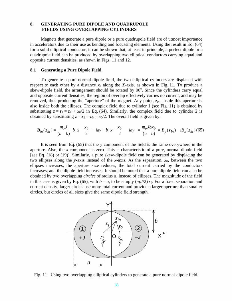
8.1 Generating a Pure Dipole Field
To generate a pure normal-dipole field, the two elliptical cylinders are displaced withrespect to each other by a distance x0 along the X-axis, as shown in Fig. 11. To produce askew-dipole field, the arrangement should be rotated by 90o. Since the cylinders carry equaland opposite current densities, the region of overlap effectively carries no current, and may beremoved, thus producing the “aperture” of the magnet. Any point, zin, inside this aperture isalso inside both the ellipses. The complex field due to cylinder 1 (see Fig. 11) is obtained bysubstituting z = z1 = zin + x0/2 in Eq. (64). Similarly, the complex field due to cylinder 2 isobtained by substituting z = z2 = zin – x0/2. The overall field is given by:
B z z zin in inino o
y xJ
a bb x
xiay b x
xiay
Jbxa b
B iB( )( ) ( )
( ) ( )=+
+
− − −
+
=
+= +
µ µ0 0 0
2 2(65)
It is seen from Eq. (65) that the y-component of the field is the same everywhere in theaperture. Also, the x-component is zero. This is characteristic of a pure, normal-dipole field[see Eq. (18) or (19)]. Similarly, a pure skew-dipole field can be generated by displacing thetwo ellipses along the y-axis instead of the x-axis. As the separation, x0, between the twoellipses increases, the aperture size reduces, the total current carried by the conductorsincreases, and the dipole field increases. It should be noted that a pure dipole field can also beobtained by two overlapping circles of radius a, instead of ellipses. The magnitude of the fieldin this case is given by Eq. (65), with b = a, to be simply (µ0J/2) x0. For a fixed separation andcurrent density, larger circles use more total current and provide a larger aperture than smallercircles, but circles of all sizes give the same dipole field strength.
–x0/
2
+x0/
2 X
Y
zin
1 2z1 z2
–J+J O
a
b
Fig. 11 Using two overlapping elliptical cylinders to generate a pure normal-dipole field.
19
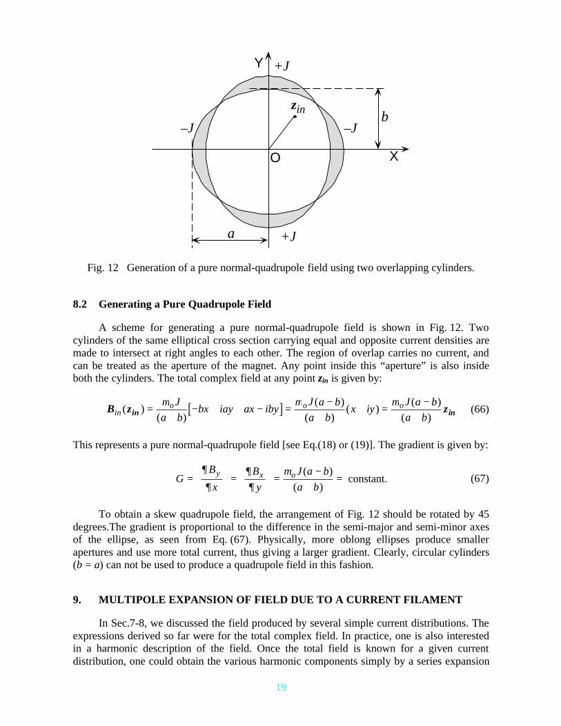
8.2 Generating a Pure Quadrupole Field
A scheme for generating a pure normal-quadrupole field is shown in Fig. 12. Twocylinders of the same elliptical cross section carrying equal and opposite current densities aremade to intersect at right angles to each other. The region of overlap carries no current, andcan be treated as the aperture of the magnet. Any point inside this “aperture” is also insideboth the cylinders. The total complex field at any point zin is given by:
[ ]B z zin inino o oJ
a bbx iay ax iby
J a ba b
x iyJ a ba b
( )( )
( )( )
( )( )
( )=
+− + + − =
−+
+ =−
+µ µ µ
(66)
This represents a pure normal-quadrupole field [see Eq.(18) or (19)]. The gradient is given by:
GB
xBy
J a ba b
y x o=
=
=
−+
=∂
∂∂∂
µ ( )( )
constant. (67)
To obtain a skew quadrupole field, the arrangement of Fig. 12 should be rotated by 45degrees.The gradient is proportional to the difference in the semi-major and semi-minor axesof the ellipse, as seen from Eq. (67). Physically, more oblong ellipses produce smallerapertures and use more total current, thus giving a larger gradient. Clearly, circular cylinders(b = a) can not be used to produce a quadrupole field in this fashion.
9. MULTIPOLE EXPANSION OF FIELD DUE TO A CURRENT FILAMENT
In Sec.7-8, we discussed the field produced by several simple current distributions. Theexpressions derived so far were for the total complex field. In practice, one is also interestedin a harmonic description of the field. Once the total field is known for a given currentdistribution, one could obtain the various harmonic components simply by a series expansion
X
Y
zin
+J
O
a
b–J
+J
–J
Fig. 12 Generation of a pure normal-quadrupole field using two overlapping cylinders.
20
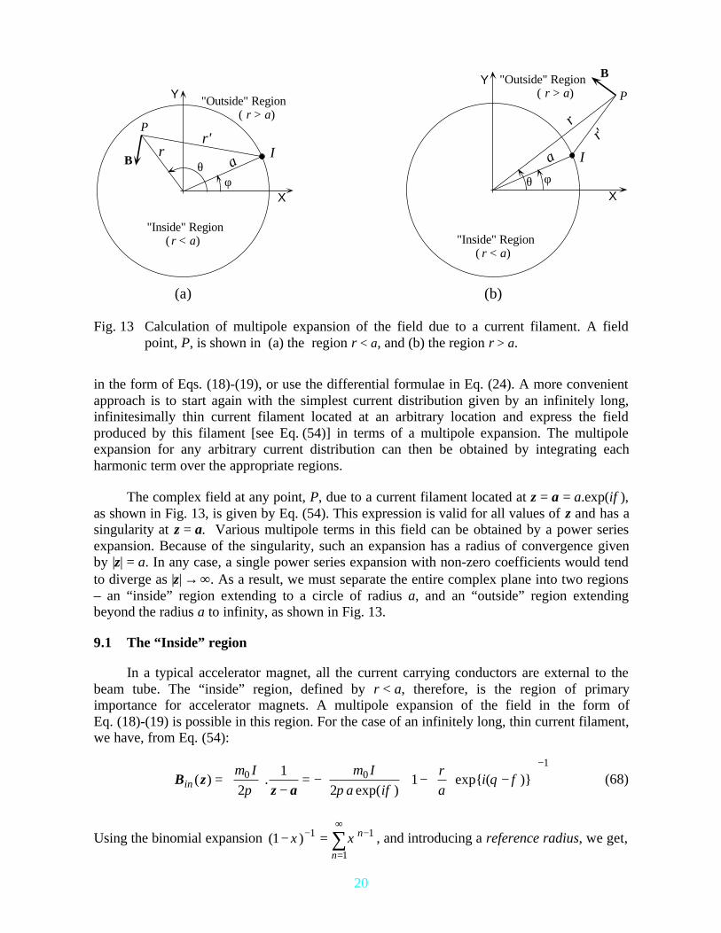
in the form of Eqs. (18)-(19), or use the differential formulae in Eq. (24). A more convenientapproach is to start again with the simplest current distribution given by an infinitely long,infinitesimally thin current filament located at an arbitrary location and express the fieldproduced by this filament [see Eq. (54)] in terms of a multipole expansion. The multipoleexpansion for any arbitrary current distribution can then be obtained by integrating eachharmonic term over the appropriate regions.
The complex field at any point, P, due to a current filament located at z = a = a.exp(iφ),as shown in Fig. 13, is given by Eq. (54). This expression is valid for all values of z and has asingularity at z = a. Various multipole terms in this field can be obtained by a power seriesexpansion. Because of the singularity, such an expansion has a radius of convergence givenby |z| = a. In any case, a single power series expansion with non-zero coefficients would tendto diverge as |z| → ∞. As a result, we must separate the entire complex plane into two regions– an “inside” region extending to a circle of radius a, and an “outside” region extendingbeyond the radius a to infinity, as shown in Fig. 13.
9.1 The “Inside” region
In a typical accelerator magnet, all the current carrying conductors are external to thebeam tube. The “inside” region, defined by r < a, therefore, is the region of primaryimportance for accelerator magnets. A multipole expansion of the field in the form ofEq. (18)-(19) is possible in this region. For the case of an infinitely long, thin current filament,we have, from Eq. (54):
B zz ain
I Ia i
ra
i( ) .exp( )
exp{ ( )}=
−
= −
−
−
−µπ
µπ φ
θ φ0 01
21
21 (68)
Using the binomial expansion ( )1 1 1
1− =− −
=
∞
∑ξ ξ n
n
, and introducing a reference radius, we get,
IB
P
rθ
φa
X
Y
r'
"Inside" Region ( r < a)
"Outside" Region ( r > a)
(a)
I
B
P
r
θ φ
a
X
Y
r'
"Inside" Region ( r < a)
"Outside" Region ( r > a)
(b)
Fig. 13 Calculation of multipole expansion of the field due to a current filament. A fieldpoint, P, is shown in (a) the region r < a, and (b) the region r > a.

21
B zz
inref
n
n
ref
nIa
inR
a R( ) exp( )= −
−
=
∞ − −
∑µπ
φ0
1
1 1
2 (69)
which is in the desired form of Eq. (9) or Eqs. (18)-(19). Comparing with Eq. (9), theamplitude and phase of the 2n-pole term are given by:
C nIa
R
a nI Iref
n
n n( ) . ;=
= + > = <
−µπ
α φπ
α φ01
20 0 for ; for (70)
where a positive value of current corresponds to current flowing along the positive Z-axis. Itshould be noted that the amplitude is always defined to be a positive quantity and any changein the field direction is absorbed in the phase angle. The NORMAL and SKEW components ofthe 2n-pole field in the “US” and “European” notations are:
B BIa
R
an
A AIa
R
an
n nref
n
n nref
n
−
−
−
−
= = −
= =
10
1
10
1
2
2
( ) ( ) . cos( )
( ) ( ) . sin( )
US European
US European
µπ
φ
µπ
φ
(71)
9.2 The “Outside” region
For the “outside” region, we expand in a power series of (a/z) instead of (z/a), since|(a/z)| < 1 in this case. Starting again with Eq. (54), we write:
B zz aout
I Ir i
ar
i( )exp( )
exp{ ( )}=
−
=
−
−
−µπ
µπ θ
φ θ0 01
21
21 (72)
Expressing the binomial expansion in the form ( )1 11
1− = +−
=
∞
∑ξ ξn
n
, we can write,
B zz zout
n
nI
n i na
( ) [cos( ) sin( )]=
+ +
=
∞
∑µπ
φ φ0
121 (73)
This series is NOT in the usual form of the multipole expansion for the field inside a magnetaperture. However, it can be seen that this expansion gives a field which reduces with distanceand converges for |z| → ∞ to Bout(z) → [µ0I/(2π z)], as expected.
It may seem puzzling at first as to why one is forced to use two different expansionsstarting from the same expression for the complex field, which is valid everywhere. It shouldbe pointed out that the division of the complex plane into “inner” and “outer” regions issomewhat artificial, and depends solely on the location of the origin, the point around whichthe series expansion is based. A point that lies in the “outside” region can be brought into the“inside” region by choosing a different origin. Starting from the series expansion for the

22
“inside” region, one can, in fact, obtain the field everywhere, including the points in the“outside” region, by a multistep process. For example, one could use the normal and skewterms at the origin, given by Eq. (71), to calculate the terms at a new origin near the periphery(but still within it) of the “inside” region, using the coordinate transformations described inSec.4 [see Eqs. (31)-(32)]. This new series expansion will be valid within a circle of a newradius, centered at the new origin. Such a circle will encompass some regions of the complexplane that were earlier in the “outer” region. This is essentially the technique of analyticcontinuation.
9.3 Effect of an Iron Yoke
In accelerator magnets, an iron yoke is almost invariably used as part of the mechanicaland magnetic design. In the design of practical magnets, one must use sophisticated numericalcalculations to include the detailed geometry as well as non-linear magnetic properties of theiron. However, analytical results can be obtained under the assumption of a constant relativepermeability, µr, and a circular aperture in an infinitely large yoke, as shown in Fig. 14. Thisgives reasonable results at low fields where the iron is not saturated.
We consider an infinitely long current filament located at a = a.exp(iφ), inside a circularaperture of radius Ryoke in the iron. The effect of the iron is obtained by applying theappropriate boundary conditions on the magnetic induction, B, and the magnetic field, H, atthe inner surface of the yoke. For calculating the field inside the aperture of the yoke, thiseffect can be described by replacing the iron with an image current of magnitude I’ located ata’ = a’.exp(iφ ’) where
( ) ( )[ ]′ = ′ = − + ′a R a I Iyoke r r2 1 1/ ; ; =µ µ φ φ (74)
Using Eq. (70), the amplitude and phase of the 2n-pole term are given by:
C n inIa
R
aa
Rinn
refn
r
r yoke
n
( )exp( ) .exp( )− = −
+
−+
−−
αµπ
µµ
φ01 2
21
11
(75)
X
Y
φ
Ryoke
a'
I
I'
a
µ0µ=µrµ0
Fig. 14 A current filament inside a circular aperture in an infinite iron yoke.

23
A comparison of Eqs. (75) and (70) shows that the presence of the iron yoke results inan increase in the field strength. Typically, for a superconducting dipole magnet, thecontribution of the iron yoke to the total field is between 10-35%. This can result insubstantial savings in the superconductor. A drawback of having a large contribution from theiron is the non-linear behaviour at higher fields, often leading to undesirable higher harmonicsdue to saturation. Such effects can be minimized to tolerable levels by a careful placement ofholes and other features in the iron yoke [13,14].
10. GENERATING A PURE 2m-POLE FIELD
We had seen in Sec.8 how simple-looking current distributions obtained by overlappingcylinders could be used to generate a pure dipole or a pure quadrupole field. Anotherapproach towards generating a field of any given multipolarity can be arrived at by looking atthe multipole expansion of the field from a thin current filament [see Sec.9].
To generate a pure 2m-pole field, the goal is to have all the terms in the expansionvanish, except for n = m. Let us assume that such a field is generated by using a thin,cylindrical current shell of radius a, similar to that shown in Fig. 7, except that the current isnot uniformly distributed. Instead, the current is a function of the azimuthal angle, φ. Thecomplex field in the region inside the current shell is obtained by integrating Eq. (69):
B zz
in
n
na ain I d( ) exp( ) ( )= −
−⌠
⌡
−
=
∞
∑µπ
φ φ φ
π
01
10
2
2(76)
In order to make all the terms except n = m vanish, it is clear that the current distribution I(φ)must be orthogonal to the function exp(–inφ ) for all n, except n = m. Clearly, such functionsare sin(nφ ) and cos(nφ ), since
cos( )cos( ) ; sin( )cos( )n m d n m dmnφ φ φ πδ φ φ φπ π
= =∫ ∫0
2
0
2
0 (77)
Therefore, for a “cosine-theta” current distribution given by
I I m( ) cos( )φ φ= 0 (78)
the complex field is given by
B zz
in
mIa a
( ) = −
−µ 0 01
2(79)
which represents a pure 2m-pole (normal) field. Similarly, for a “sine-theta” current distri-bution given by I I m( ) sin( )φ φ= 0 , the field is a skew 2m-pole field.
Unfortunately, neither the intersecting cylinders, nor the “cosine-theta” distributions canbe accurately reproduced in practice. For example, the intersecting cylinders have sharp edges

24
that must be rounded off in practice, leading to unacceptable harmonic distortions. In thedesign of conductor-dominated magnets (such as superconducting magnets), one has toapproximate these distributions with several turns of a finite sized conductor carrying a givencurrent. This has led to the concept of “current blocks” approximation to the “cosine-theta”distribution. In this approach, a nearly pure multipole field is generated by employing one ormore “current blocks”. Each of the blocks is formed by one or more turns of a conductor witha fixed cross section. The current is usually kept the same in each of the blocks for practicalreasons. A description of this approach can be found in reference [15]. As an example, thecoils for the arc dipole magnets for the Relativistic Heavy ion Collider (RHIC), being built atthe Brookhaven National Laboratory, consist of four current blocks with 9, 11, 8 and 4 turns[16]. Such a design attempts to zero out several of the lower order harmonics and also reducethe remaining higher order terms to negligible levels.
11. CURRENT SYMMETRIES AND ALLOWED HARMONICS
For a general current distribution, all harmonic terms in the multipole expansion of thefield would be present. The current distributions in accelerator magnets have varioussymmetry properties depending on the type of the magnet. These symmetries imply that thenormal and/or skew components of certain harmonics must vanish [17]. Such harmonic termsare referred to as the unallowed terms. The harmonics that can possibly be non-zero arecalled the allowed terms. It should be noted that a particular term may be allowed, but absentdue to a careful design of the magnet. On the other hand, a particular term may be unallowed,but present in a magnet due to violation of the relevant symmetry as a result of constructionerrors. In this section, we shall discuss the various symmetries and derive the correspondingallowed terms.
We shall assume that the current density, J, is a function of the azimuthal angle only.This assumption is valid for the current blocks formed with finite sized conductors. Based onEq. (69), the amplitude and phase of the 2n-pole term are given by:
∫C n in J e dnin( )exp( ) ( )− ∝ −α φ φφ
π
0
2(80)
The normal and the skew components are proportional to the real and the imaginaryparts of the integral in Eq. (80). The fundamental symmetry in a 2m-pole magnet is a 2m-foldrotational antisymmetry, since the north and south poles of such a magnet are interchangedunder a rotation by (π /m) radians. In addition, a magnet may have left-right, or top-bottomsymmetry (or antisymmetry) if the X-Y axes are properly oriented.
11.1 Allowed harmonics in a 2m-pole magnet
It was shown in Sec.10 that a pure 2m-pole field is produced by a cos(mθ ) or a sin(mθ )distribution of current. Such a current distribution is antisymmetric under a rotation by (π /m)radians and is symmetric under a rotation by (2π /m) radians. Even when the cos(mθ )distribution is approximated by current blocks, this rotational symmetry is still preserved for a2m-pole magnet. The current density at any azimuthal angle φ + π /m is opposite that at φ, andso on, as shown in Fig. 15. Using this fact, the integral in Eq. (80) can be written as a sum of2m terms:

25
∫C n in J e e e e dnin in m in m
mi m m( )exp( ) ( ) [ ]/ /
/( ) /α φ φφ π π
ππ∝ − + + − −1 2
0
2 1 L (81)
or, ∫C n in J e de
en
inm in
in m( )exp( ) ( )
/
/α φ φφ
π π
π∝
⋅−
+
0
21
1(82)
Since n is always an integer, exp(2inπ) = 1 and the right hand side in the above integralvanishes, unless the denominator also vanishes. This requires that n must be an odd multipleof m. Thus, for a dipole magnet (m = 1), only terms with n = 1,3,5,... are allowed. For aquadrupole magnet (m=2), terms with n = 2,6,10,... are allowed, and so on.
11.2 “Top-Bottom” Symmetry or Anti-symmetry
A “top-bottom” symmetry about the X-axis implies J(2π – φ ) = J(φ ), as shown inFig. 16. In this case, Eq. (80) can be written as:
∫ [ ]∫ ∫C n in J e d J e e d J n dnin in in( )exp( ) ( ) ( ) ( )cos( )( )α φ φ φ φ φ φ φφ
πφ π φ
π π∝ = + =−
0
22
0 0(83)
The result of integration has no imaginary part in this case. This implies that all the skewterms vanish and only the normal terms are allowed as a result of the “top-bottom” symmetryin the current distribution. It is obvious that the current distribution in all normal magnets,such as a normal dipole, a normal quadrupole, etc. must have top-bottom symmetry.
φφ+π/m J(φ)
J(φ+π/m) = –J(φ)
π/m
2π/m3π/m
(2m−1)π/m
X
YJ(φ+2π/m) = J(φ)
(2m−2)π/mφ+
2π/ m
Fig. 15 Rotational symmetry of current density in a 2m-pole magnet.

26
The case of the “top-bottom” antisymmetry is similar, except that the current densitysatisfies J(2π – φ ) = –J(φ ). The integral in Eq. (80) becomes,
∫ [ ]∫ ∫C n in J e d J e e d i J n dnin in in( )exp( ) ( ) ( ) ( )sin( )( )α φ φ φ φ φ φ φφ
πφ π φ
π π∝ = − =−
0
22
0 0(84)
The result of integration has no real part in this case. This implies that all the normal termsvanish and only the skew terms are allowed as a result of the “top-bottom” antisymmetry inthe current distribution. All skew magnets, such as a skew dipole, a skew quadrupole, etc.have a “top-bottom” antisymmetry.
11.3 “Left-Right” Symmetry or Anti-symmetry
A “left-right” symmetry about the Y-axis implies J(π – φ ) = J(φ ), as shown in Fig. 17.In this case, Eq. (80) can be written as:
[ ]∫ [ ]∫C n in J e e d J e e dnin in in n in( )exp( ) ( ) ( ) ( )( )
/
/
/
/
α φ φ φ φφ π φ
π
πφ φ
π
π
∝ + = + −−
−
−
−2
2
2
2
1 (85)
∫
∫
C n in i J n d n
C n in J n d n
n
n
( )exp( ) ( )sin( )
( )exp( ) ( )cos( )
/
/
/
/
α φ φ φ
α φ φ φ
π
π
π
π
∝
∝
−
−
2
2
2
2
for ODD
for EVEN
Left-Right Symmetry (86)
J(φ)
φ
2π−φ
J(2π−φ )= J(φ)
X
Y
Fig. 16 “Top-bottom” symmetry in the current distribution.

27
The result of integration has no real part for odd multipoles and has no imaginary part foreven multipoles. This implies that all the odd normal terms (such as the normal dipole, thenormal sextupole, etc.) and all the even skew terms (such as the skew quadrupole, the skewoctupole, etc.) vanish as a result of the “left-right” symmetry in the current distribution. Allthe normal magnets of even order, such as a normal quadrupole, and all the skew magnets ofodd order, such as the skew dipole, have this type of current symmetry.
Similarly, a “left-right” antisymmetry implies J(π – φ ) = –J(φ ). In this case, Eq. (80)can be written as:
[ ]∫ [ ]∫C n in J e e d J e e dnin in in n in( )exp( ) ( ) ( ) ( )( )
/
/
/
/
α φ φ φ φφ π φ
π
πφ φ
π
π
∝ − = − −−
−
−
−2
2
2
2
1 (87)
∫
∫
C n in i J n d n
C n in J n d n
n
n
( )exp( ) ( )sin( )
( )exp( ) ( )cos( )
/
/
/
/
α φ φ φ
α φ φ φ
π
π
π
π
∝
∝
−
−
2
2
2
2
for EVEN
for ODD
Left-Right Antisymmetry (88)
The result of integration has no real part for even multipoles and has no imaginary part forodd multipoles. This implies that all the even normal terms (such as the normal quadrupole,the normal octupole, etc.) and all the odd skew terms (such as the skew dipole, the skewsextupole, etc.) vanish as a result of the “left-right” antisymmetry in the current distribution.All the normal magnets of odd order, such as a normal dipole, and all the skew magnets ofeven order, such as the skew quadrupole, have this type of current symmetry.
J(φ)
φπ−φ
J(π−φ )= J(φ)
X
Y
Fig. 17 “Left-Right” symmetry in the current distribution.
28
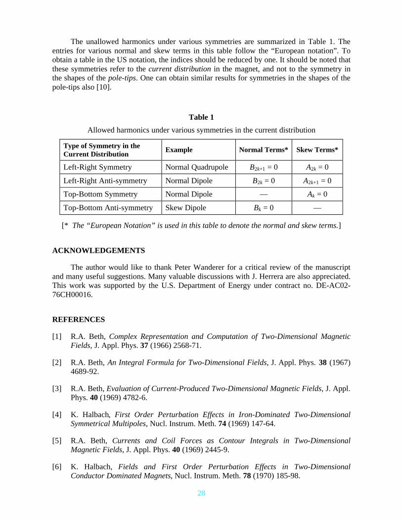
The unallowed harmonics under various symmetries are summarized in Table 1. Theentries for various normal and skew terms in this table follow the “European notation”. Toobtain a table in the US notation, the indices should be reduced by one. It should be noted thatthese symmetries refer to the current distribution in the magnet, and not to the symmetry inthe shapes of the pole-tips. One can obtain similar results for symmetries in the shapes of thepole-tips also [10].
Table 1
Allowed harmonics under various symmetries in the current distribution
Type of Symmetry in theCurrent Distribution
Example Normal Terms* Skew Terms*
Left-Right Symmetry Normal Quadrupole B2k+1 = 0 A2k = 0
Left-Right Anti-symmetry Normal Dipole B2k = 0 A2k+1 = 0
Top-Bottom Symmetry Normal Dipole — Ak = 0
Top-Bottom Anti-symmetry Skew Dipole Bk = 0 —
[* The “European Notation” is used in this table to denote the normal and skew terms.]
ACKNOWLEDGEMENTS
The author would like to thank Peter Wanderer for a critical review of the manuscriptand many useful suggestions. Many valuable discussions with J. Herrera are also appreciated.This work was supported by the U.S. Department of Energy under contract no. DE-AC02-76CH00016.
REFERENCES
[1] R.A. Beth, Complex Representation and Computation of Two-Dimensional MagneticFields, J. Appl. Phys. 37 (1966) 2568-71.
[2] R.A. Beth, An Integral Formula for Two-Dimensional Fields, J. Appl. Phys. 38 (1967)4689-92.
[3] R.A. Beth, Evaluation of Current-Produced Two-Dimensional Magnetic Fields, J. Appl.Phys. 40 (1969) 4782-6.
[4] K. Halbach, First Order Perturbation Effects in Iron-Dominated Two-DimensionalSymmetrical Multipoles, Nucl. Instrum. Meth. 74 (1969) 147-64.
[5] R.A. Beth, Currents and Coil Forces as Contour Integrals in Two-DimensionalMagnetic Fields, J. Appl. Phys. 40 (1969) 2445-9.
[6] K. Halbach, Fields and First Order Perturbation Effects in Two-DimensionalConductor Dominated Magnets, Nucl. Instrum. Meth. 78 (1970) 185-98.

29
[7] R.A. Beth, Complex Methods for Three-Dimensional Magnetic Fields, Proc. 1971Particle Accelerator Conference, Chicago, USA, March 1-3, 1971.
[8] G. Guignard, The General Theory of All Sum and Difference Resonances in a Three-Dimensional Magnetic Field in a Synchrotron, Report CERN 76-06, March 23, 1976.
[9] W. Fischer and M. Okamura, Parameterization and Measurements of Helical MagneticFields, Proc. 1997 Particle Accelerator Conference, Vancouver, Canada, May 12-16,1997 (to be published).
[10] W.C. Elmore and M.W. Garrett, Measurement of Two-Dimensional Fields. Part I:Theory, Rev. Sci. Instrum. 25 (1954), No. 5, 480-5.
[11] P.J. Bryant, Basic Theory for Magnetic Measurements, Proc. CERN Accelerator Schoolon Magnetic Measurement and Alignment, Montreux, Switzerland, March 16-20, 1992,(CERN Report 92-05) pp.52-69.
[12] See, for example, Methods of Theoretical Physics, P.M. Morse and H. Feshbach,McGraw Hill, New York, Part I, p.38.
[13] P.A. Thompson et al., Iron Saturation Control in RHIC Dipole Magnets, Proc. 1991Particle Accelerator Conference, San Francisco, USA, May 6-9, 1991, in IEEE Conf.Record 91CH3038-7, pp.2242-4.
[14] R. Gupta et al., Field Quality Improvements in Superconducting Magnets for RHIC,Proc. 4th European Particle Accelerator Conference, London, UK, June 27-July 1, 1994.
[15] K.-H. Meβ and P. Schmüser, Superconducting Accelerator Magnets, Proc. CERNAccelerator School on Superconductivity in Particle Accelerators, Hamburg, Germany,May 30-June 3, 1988 (CERN Report 89-04), pp.87-148.
[16] P.A. Thompson et al., Revised Cross Section for RHIC Dipole Magnets, Proc. 1991Particle Accelerator Conference, San Francisco, USA, May 6-9, 1991, in IEEE Conf.Record 91CH3038-7, pp.2245-7.
[17] J.C. Herrera, Basic Symmetries in ISABELLE Magnets, Magnet Test Group NoteNo. 110, June 3, 1981, Brookhaven National Laboratory, Upton, New York 11973.