Contents lists available at ScienceDirect

Electrical Power and Energy Systems

journal homepage: www.elsevier.com/locate/ijepes

Virtual storage plant offering strategy in the day-ahead electricity market

Kristina Pandžića, Hrvoje Pandžićb,⁎, Igor Kuzleba Croatian Transmission System Operator – HOPS Ltd., CroatiabDepartment of Energy and Power Systems, Faculty of Electrical Engineering and Computing, University of Zagreb, Croatia

A R T I C L E I N F O

Keywords:Virtual storage plantEnergy storageBilevel programmingMathematical problem with equilibriumconstraints

A B S T R A C T

Energy storage is gaining an important role in modern power systems with high share of renewable energysources. Specifically, large-scale battery storage units (BSUs) are an attractive solution due to their modularity,fast response and ongoing cost reduction.

This paper aims to formulate, analyze and clarify the role of merchant-owned BSUs in the day-ahead elec-tricity market. It defines virtual storage plant (VSP) as a set of BSUs distributed across the network. A VSPoffering model is formulated as a bilevel program in which the upper-level problem represents the VSP profitmaximization and operation, while the lower-level problem simulates market clearing and price formation. Thismathematical problem with equilibrium constraints (MPEC) is converted into a mixed-integer linear program(MILP). This is afterwards expanded to a game of multiple VSPs formulating an equilibrium problem withequilibrium constraints (EPEC), which is solved using the diagonalization procedure.

The proposed model is applied to an updated IEEE RTS-96 system. We evaluate the impact VSPs have on thelocational marginal prices and compare the coordinated approach (all BSUs operated under a single VSP), i.e. theMPEC formulation, to the competitive approach (multiple VSPs competing for profit), i.e. the EPEC formulation.

1. Introduction

1.1. Motivation

The increasing share of renewable energy sources (RES) is changingthe paradigm of modern power systems. The term power itself indicatesa constant balance between demand and supply. However, an increasedshare of non-controllable RES, i.e. solar and wind, results in less dis-patchable capacity at the disposal to the system operator. Thus, thetechnical ability to meet the uncertain net demand is reducing becauseRES output can vary within a market interval [1]. Many studies reportthat intermittent non-dispatchable RES increase reserve requirement,e.g. Italian historical data analyzed in [2] report a decrease of energyprices and increase of reserve costs as a result of the RES integration.These technical and economic conditions make large-scale energy sto-rage solutions attractive, as they enable switching to the energy systemparadigm, as opposed to the power system paradigm. As opposed to thecurrent power system paradigm, where generation and demand need tobe balanced at each point in time, in an energy system, generation anddemand need to be balanced over a longer time period, e.g. hours,while energy storage acts as a buffer that voids the short-term gen-eration-load imbalances. In other words, energy storage enables secure

and stable power system operation even without the constant genera-tion-demand balance since it acts as a generation and demand assetinterchangeably. Rassmussen et al. [3] claim that large distributedenergy storage would enable covering the entire electricity demand inEurope using only RES. Related to this, electricity generation of windturbines is already reaching high levels. In 2015, Danish wind turbinesgenerated an equivalent of 42 percent of the overall electricity demandin that country [4].

Regulative authorities have not yet issued clear regulating me-chanisms governing the use of energy storage in electricity markets.Joint European Association for Storage of Energy and European EnergyResearch Alliance recommendations for European Energy StorageTechnology Development Roadmap towards 2030 [5] recognizes thatenergy storage technology can be used to provide regulated services tosystem operators and non-regulated services in electricity markets (seethe model presented in [6]). In the USA, Federal Energy RegulatoryCommission (FERC) has issued orders to help facilitate energy storagein regulated markets. FERC Order 555 issued a pay-per-performanceincentive for resources that can provide quicker and more preciseresponses to frequency regulation signals. This enables energystorage technologies which outperform the conventional regulationproviders, such as gas- and coal-fired power plants, to receive higher

https://doi.org/10.1016/j.ijepes.2018.07.006Received 14 January 2018; Received in revised form 26 May 2018; Accepted 5 July 2018

⁎ Corresponding author.E-mail addresses: kristina.pandzic@hops.hr (K. Pandžić), hrvoje.pandzic@fer.hr (H. Pandžić), igor.kuzle@fer.hr (I. Kuzle).

Electrical Power and Energy Systems 104 (2019) 401–413

0142-0615/ © 2018 Elsevier Ltd. All rights reserved.

T

remuneration. An evaluation of the utility of energy storage for dif-ferent market paradigms and ownership models is available in [7].

The main disadvantages of conventional large-scale energy storage,i.e. pumped hydro and compressed air energy storage, are geographicalconstraints and bulkiness. Due to these limitations, conventional sto-rage technologies are less suitable than modular storage devices thatcan be installed at virtually any location without a significant ecologicalfootprint. A review of the current state of energy storage technologiesindicates that batteries are generally a versatile energy storage tech-nology that can be installed at almost any location [8]. A common grid-scale battery technology today is lithium-ion, which is suitable forproviding frequency regulation [9]. Energy-to-power ratio of lithium-ion battery installations is usually lower than 1 and installed capacitiesare much lower than the ones of traditional energy storage, i.e. pumpedhydro [10]. On the other hand, NaS batteries are more suitable forcongestion relief as their energy-to-power ratio is 7 [11]. On top of this,the cost of batteries has been reducing due to their use in electric ve-hicles [12]. A review on battery energy storage technologies is availablein [13].

Large-scale use of battery storage has a wide range of applications,providing different values to the power system. Battery storage units(BSUs) can help in peak shaving [14] and increasing the system flex-ibility and reliability providing power regulation services [15]. Fast-response energy storage, such as BSU, has the potential to replace fast-ramping generation resources [16]. Economics of transmission or ca-pacity investment deferral are addressed in [17]. Therefore, the de-velopment of energy storage technology, especially battery technology,might offer solutions for many critical challenges in smart grids[18,19]. Combining these applications reduces the payback periodmaking the investment more attractive.

Storage operation highly depends on its ownership. For instance,Terna’s BSUs are used to ensure safety and cost-effective managementof the Italian transmission grid [9]. In a vertically integrated utility,BSUs are used to reduce the overall operating cost [20]. Finally,

merchant-owned BSU is operated in a way to maximize its profit [21].In case multiple BSUs are operated by different owners, they competewith each other to make profit. This resembles an equilibrium problemwith equilibrium constraints (EPEC), i.e. a multiple-leader-common-follower game, as introduced in [22]. EPEC structure is particularlycommon in the analysis of deregulated electricity markets [23,24],where players maximize their benefit in the form of mathematicalproblems with equilibrium constraints, MPECs, e.g. [25], while ad-hering to the same market-clearing rules. For instance, in [26] an EPECmodel is derived to find equilibria reached by strategic producers in apool-based transmission-constrained electricity market using KKT con-ditions, while in [27] the authors use diagonalization method to findmultiple equilibria of generator maintenance schedules in electricitymarket environment.

The goal of the presented model is to formulate, model and analyzestorage operation in the day-ahead electricity market. A VSP owns andoperates its BSUs distributed across the system in order to maximizetheir overall market performance. It derives an optimal strategy cen-trally and sends control signals to all its BSUs to charge/discharge.

1.2. Literature review

Generally, integration of energy storage in power systems can beobserved either from the system-wide perspective or the merchantperspective. The system-wide perspective is usually modeled as a unitcommitment model whose goal is to minimize overall system operatingcosts, regardless on the profit an energy storage is making. An exceptionin the literature is [28], which minimizes the overall system costs whileensuring the profitability of a merchant-owned energy storage. On theother hand, there are models which take perspective of a storage owner,thus aiming at maximizing the profit a storage is making in electricitymarkets. In these models, energy storage can be a significant marketplayer able to affect the market prices, i.e. price maker models, or its

Nomenclature

Sets

ΩB set of piecewise linear segments of each generating unit’soffer curve, indexed by b.

ΩC set of piecewise linear segments of each bus’ demand bidcurve, indexed by c.

ΩH set of BSUs, indexed by h.ΩI set of generating units, indexed by i.ΩJ set of VSP owners, indexed by j.ΩL set of transmission lines, indexed by l.ΩS set of buses, indexed by s.ΩT set of hours, indexed by t .ΩW set of wind farms, indexed by w.

Binary variables

xt h,ch BSU charging status (1 if BSU h is charging during hour t,

0 otherwise).xt h,

dis BSU discharging status (1 if BSU h is discharging duringhour t , 0 otherwise).

Continuous variables

dt s c, , power consumption on segment c at s during hour t (MW).gt i b, , power output on segment b of generator i during hour t

(MW).kt w, power output of wind farm w during hour t (MW).

pft s m, , power flow through line −s m during hour t (MW).qt h,

ch power purchased by BSU h during hour t (MW).qt h,

dis power sold by BSU h during hour t (MW).soet h, state of energy of BSU h during hour t (MWh).αt h,

ch charging bid of BSU h during hour t (MW).αt h,

dis discharging offer of BSU h during hour t (MW).θt s, voltage angle of bus s during hour t (rad).λt s h, ( ) locational marginal price at bus s where BSU h is located

($/MW).

Parameters

chhmax charging capacity of BSU h (MW).

dishmax discharging capacity of BSU h (MW).

dt s c, ,max capacity of demand block c at bus s during hour t (MW).

ηhch charging efficiency of BSU h.

ηhdis discharging efficiency of BSU h.

gi b,max capacity of offering block b of generator i (MW).

kt w,max available wind generation of wind farm w (MW).

λhch bidding price of BSU h ($/MW).

λhdis offering price of BSU h ($/MW).

λs c,D bidding price of demand block c at bus s ($/MW).

λi b,G offering price of block b of generator i ($/MW).

pfs m,max transmission capacity of line −s m (MW).

soehmax energy capacity of BSU h (MWh).

soehmin minimum energy stored in BSU h (MWh).

sussm susceptance of line connecting nodes s and m (S).

K. Pandžić et al. Electrical Power and Energy Systems 104 (2019) 401–413

402

capacity can be relatively low as compared to other generating anddemand capacities, which means the storage is a price taker.

1.2.1. System-wide studiesThe authors of [29] assess the potential of energy storage to eco-

nomically decrease wind curtailment and/or system costs. The authorsreport that batteries with higher power rating result in less wind cur-tailment, but also require lower installation costs. The sensitivity ana-lysis indicates that the most relevant parameters are the existence ofsubsidies, the installation cost of transmission lines, battery degradationand life cycle duration.

An approximate unit commitment model based on load durationcurve is presented in [30]. System states framework is used to preservethe storage intertemporal dependencies. Since the same system statesmight have different storage states of energy, which depend on thestates before and after the current time period, the authors use thedifference in state of energy, and not stored energy, as variables. Theproposed method improves computational tractability by 90% ascompared to the chronological hour-by-hour models, while causing anerror of less than 2%.

Paper [31] uses stochastic programming models to derive optimalunit commitment policy with pump storage plants as an importantstorage technology in which the investments are expected to increase.

In [20], the authors present a near-optimal three-stage technique forsiting and sizing of battery energy storage in transmission network. Theauthors conclude that optimal storage locations are near wind farms oralong the congested corridors of a network.

A framework for storage portfolio optimization in transmission-constrained power networks is proposed in [32]. The model optimizesstorage operation and siting given a fixed technology portfolio. Ad-ditionally, the authors optimize the portfolio itself, thus demonstratingthe importance of choosing a proper technology.

Paper [33] presents a study on utilizing energy storage to manageintra-hour variability of the net load. A standard unit commitmentmodel is implemented in PLEXOS, with addition of primary, secondaryand tertiary reserve provision. Implementation of the model to theexpected plant portfolio in Irish system in 2025 reveals that integrationof storage should lead to 15% less cycling of conventional units and upto 40% savings in operating costs.

1.2.2. Price-taking merchant-owned storageMerchant-owned energy storage can be used to support the local

renewable generation or independently act in electricity markets. In[34] the authors propose a joint bidding mechanism of a wind farm anda pumped hydro plant in the day-ahead and ancillary service markets. Aprofit maximization model of a virtual power plant that includes energystorage is proposed in [35]. This model accounts for bilateral contractswhile maximizing the profit in the day-ahead electricity market. A si-milar study [36] shows that using batteries to compensate for inter-mittent and variable generation results in a smoother overall generationcurve.

As opposed to [34–36], where energy storage is used to supportrenewable generation, the authors in [37] present a profit maximiza-tion model for a price-taker storage unit that participates in energy andreserve day-ahead market and energy hour-ahead market. Uncertainparameters are the price of power and reserve in the hour-aheadmarket, and the actual reserve utilization. The values for these para-meters are obtained by presolving a stochastic unit commitment modelfor different realizations of wind. The authors demonstrate the im-portance of considering the uncertainty of market prices (due to un-certain nature of wind) in the presented independent energy storageprofit maximization model. Paper [38] also deals with energy storageeconomics when participating in arbitrage and regulation serviceswithin different markets. The case study results show that high poten-tial revenues could be generated from ancillary services market. Abackwards induction approach is employed in [39] to derive optimal

bidding strategy of a battery storage operator. The authors consider thestorage device exhaustable with a limited number of cycles and life-time.

The authors of [40] present a case study to demonstrate that storagetechnologies may have competitive advantage over the peaking gen-erators, due to the ability to earn revenue outside of extreme peakevents. The main driver for storage options in an energy-only electricitymarket is extreme prices, which in turn is dependent on capacity re-quirements.

Paper [41] uses a portfolio of energy trade strategies to determinethe value of arbitrage for energy storage across the European markets.The results show that arbitrage opportunities exist in less integratedmarkets, characterized by significant reliance on energy imports andlower level of market competitiveness.

The authors of [42] provide a comprehensive stochastic energystorage valuation framework which allows a storage system to providemultiple services simultaneously, i.e., the frequency regulation serviceand energy shifting service are co-optimized in the market operations.An operational optimization model is developed to determine the sto-rage system’s optimal dispatch sequences with a frequency regulationservice price forecasting model. Simulation results show that the ma-jority of the revenue comes from regulation services.

1.2.3. Price-making merchant-owned storageIn [21], the authors assess the impact of strategic energy storage

behavior in a nodal electricity market. The results indicate that thestorage profit maximization goal is not always in line with the socialwelfare improvement. Namely, the storage aims to retain the pricevolatility among hours in order to maximize its profit.

A bilevel formulation of a coordinated scheduling of multiple sto-rage units is presented in [43]. The upper-level problem sets optimalmarket bids and offers for each storage unit, while the lower-levelproblem simulates market clearing procedure. The initial formulation isconverted to MPEC and linearized using the Karush–Kuhn–Tucker(KKT) conditions of the lower-level problem. The paper also containsstochastic and basic robust (maximizing the profit of the least profitablescenario) reformulations of the upper-level problem. The importantconclusions are that the transmission congestion is usually beneficialfor energy storage profit and that locations of individual storage unitsaffect their coordinated scheduling and profit.

The authors of [44] propose a bilevel formulation where the upper-level problem seeks to maximize merchant storage arbitrage profit,while the lower-level problem simulates market clearing. The lower-level problem is a stochastic problem, depending on wind scenarios.The paper specifically analyzes the impact of the thermal generatorflexibility on storage profit. The authors illustrate how storage takesadvantage of different system conditions. The case study shows that acongested transmission grid enables storage to exercise spatio-temporalarbitrage, bringing much more revenue as compared to only exploitinglimited ramping constraints of conventional generators.

Paper [45] examines the impact storage has on generator companyprofit increment due to strategic bidding. The authors exploit the bi-level structure, where the upper-level problem maximizes the totalprofit of generating companies. The lower-level problem is a simulationof transmission-unconstrained market clearing procedure. The con-ducted case study indicates that energy storage diminishes the possi-bility of generating companies to exercise market power at high-de-mand hours, but increases it at off-peak periods. However, thereduction at peak periods is higher than the increase in off-peak periodsdue to the larger slope of the strategic marginal cost curve. Therefore,energy storage is beneficial to the bidding side, as it helps preservingthe bidding side surplus.

The authors of [46] propose a multi-period equilibrium problemwith equilibrium constraints to study strategic behavior of variousgenerators. The model considers energy storage systems as price makersin the energy market and their impact on the market equilibrium is

K. Pandžić et al. Electrical Power and Energy Systems 104 (2019) 401–413

403

thoroughly analyzed. The nonlinear complementarity constraints arehandled using a reformulation technique. The paper [47] proposes abilevel equilibrium model to study market equilibrium interactionsbetween energy storage and wind and conventional generators.

Paper [48] demonstrates that in some market structures energystorage can reduce social welfare, which contradicts conventional opi-nion of reducing the welfare losses by adding firms to an imperfectlycompetitive market. These findings have important implications forstorage development and storage-related policies.

A case study on integration of energy storage in German electricitymarket is presented in [49]. The results indicate that energy storagereduces price spikes and producer surplus. The authors conclude thatenergy storage investments are not attractive to companies that alreadyown generation facilities.

1.3. Scope and contributions

The model proposed in this paper falls in the category of merchant-owned energy storage operation problems. While papers [21,48] arefocused on energy storage impact on social welfare, [43,44] on theimpact of uncertainty on energy storage operation, [44–49] on inter-action between generators and energy storage, this paper aims at fillingthe literature gap on interaction between energy storage companies, i.e.VSPs. Specifically, we determine the benefits of a longer look-aheadhorizon than a single day, the loss of profit when having independentVSPs competing in the day-ahead market and the consequences of notconsidering the market decisions of other VSPs when bidding in theday-ahead market.

The presented model assumes that VSP is a price maker and makesprofit in the day-ahead market by performing arbitrage. We employbilevel programming in order to model the relationship between theVSP operator’s optimal bidding problem and the market operator’smarket clearing problem. These two problems interact in a way that theupper-level problem decides on VSPs bidding quantities (and prices),while the lower-level problem performs market clearing considering theupper-level decisions. The outcome of the lower-level problem are,among others, locational marginal prices (LMPs), which are used in theupper-level problem to calculate the VSP profit of the VSP.

We present three different models that depict different market op-eration of storage units. The first model is an MPEC that optimizesbidding quantities of a VSP owning a number of BSUs. It is assumed thatoffering and bidding prices are set to zero and to the market cap value,respectively. The second MPEC is also focused on a single-entity ownedstorage, but apart from the quantities, the storage operator sets theoffering and bidding prices as well. Finally, the third model is an EPECwhere different VSPs compete for profit by scheduling their BSUs. ThisEPEC is a multiple-leader-common-follower game, where different VSPowners are the leaders subject to the same follower – the market.

The contributions of the paper are summarized as follows:

1. Formulation of a VSP price and quantity offer model (MPEC) and itscomparison to the quantity-only offer model.

2. Analysis and quantitative evaluation of the look-ahead horizon ofthe VSP operation model. Namely, even when operating a daily-cycle storage, a look-ahead horizon longer than a single day mightbe required.

3. Formulation of a multiple VSP model (EPEC), where a diag-onalization method is utilized to evaluate possible equilibria whendifferent storage owners compete to maximize their profit.

4. Comparison of the EPEC approach (BSUs divided among multipleVSPs) to the case of a single VSP, i.e. all BSUs operated by a singleVSP.

The presented models and analysis should be interesting to energy

storage investors, operators of energy storage facilities, aggregators ofdistributed storage units, and balance responsible parties.

2. Formulation

This paper employs formulations to model each of the followingsettings:

1. Quantity-only MPEC model, i.e. offering at zero price and bidding atthe market cap price, presented in Section 2.2.

2. Price-quantity MPEC model, presented in Section 2.3.3. EPEC model, presented in Section 3.1.

The main notation used throughout the paper is listed at the beginningof the paper for a quick reference. Dual variables of the lower-levelproblem constraints are stated after a colon in the corresponding con-straint.

2.1. Quantity-only model formulation

.

∑ ∑ −∈ ∈

λ q qmax ·( )t h

t s h t h t hΩ Ω

, ( ) ,dis

,ch

T H (1)

subject to:

= + − ∀ ∈ ∈−soe soe t q η tq

ηt hΔ · · Δ · Ω , Ωt h t h t h h

t h

h, 1, ,

ch ch ,dis

disT H

(2)

+ ⩽ ∀ ∈ ∈x x t h1 Ω , Ωt h t h,ch

,dis T H (3)

⩽ ⩽ ∀ ∈ ∈soe soe soe t hΩ , Ωh t h hmin

,max T H (4)

∑ ∑ ∑ ∑ ∑

∑ ∑ ∑ ∑ ∑

+

− −

∈ ∈ ∈ ∈ ∈

∈ ∈ ∈ ∈ ∈

λ d λ q

λ g λ q

max · ·

· ·t s c

s c t s ct h

h t h

t i bi b t i b

t hh t h

Ω Ω Ω,

D, ,

Ω Ω

ch,ch

Ω Ω Ω,G

, ,Ω Ω

dis,dis

T S C T H

T I B T H (5)

subject to:

∑ ∑ ∑ ∑ ∑ ∑

∑ ∑ ∑

− − − + −

= − − ∀ ∈ ∈

∈ ∈ ∈ ∈ ∈

−

∈

+

∈ ∈ ∈

k q g pf pf

d q λ t sΩ , Ωw

t wh

t hi b

t i bl

t ll

t l

s ct s c

ht h t s

Ω,

Ω,dis

Ω Ω, ,

Ω,

Ω,

Ω Ω, ,

Ω,ch

,T S

W(S) H(S) I(S) B L(S) L(S)

S C H(S) (6)

= − ∀ ∈ ∈ ∈pf sus θ θ β t l l s m·( ): Ω , Ω , { , }t l s m t s t m t l, , , , ,T L (7)

− ⩽ ⩽ ∀ ∈ ∈pf pf pf β β t l: , Ω , Ωl t l l t l t lmax

,max

,min

,max T L

(8)

⩽ ⩽ ∀ ∈ ∈ ∈g g γ γ t i b0 : , Ω , Ω , Ωt i b i b t i b t i b, , ,max

, ,min

, ,max T I B

(9)

⩽ ⩽ ∀ ∈ ∈ ∈d d σ σ t s c0 : , Ω , Ω , Ωt s c t s c t s c t s c, , , ,max

, ,min

, ,max T S C (10)

⩽ ⩽ ∀ ∈ ∈q dis x ϕ ϕ t h0 · : , Ω , Ωt h h t h t h t h,dis max

,dis

,dmin

,dmax T H

(11)

⩽ ⩽ ∀ ∈ ∈q ch x ϕ ϕ t h0 · : , Ω , Ωt h h t h t h t h,ch max

,ch

,cmin

,cmax T H

(12)

⩽ ⩽ ∀ ∈ ∈k k η η t w0 : , Ω , Ωt w t w t w t w, ,max

,min

,max T W

(13)

− ⩽ ⩽ ∀ ∈ ∈π θ π μ μ t s: , Ω , Ωt s t s t s, ,max

,max T S (14)

= ∀ ∈θ μ t0: Ωt s t,ref T

1 (15)

Objective function (1) maximizes the profit of the VSP. LMP at thebus to which a BSU is connected is equal to the negative of λt s, , the dualvariable of the power balance Eq. (6) calculated endogenously in thelower level problem. BSU’s profit comes from the difference of LMPs

K. Pandžić et al. Electrical Power and Energy Systems 104 (2019) 401–413

404

when electricity is sold and purchased in the market. Therefore, theBSU’s revenue is highly dependent on the LMP profile at the connectingbus.

The objective function (1) is subject to the upper-level constraintsrepresenting storage operation (2)–(4) and a lower-level problem si-mulating market clearing procedure (5)–(15).

Constraint (2) determines the current state of energy of a BSU basedon its value in the previous time period, as well as charging and dis-charging amounts and efficiencies during the current time period. Thisequation considers both charging and discharging efficiencies. Con-straint (3) forbids simultaneous charging and discharging of batterystorage. Constraint (4) limits the state of energy of a BSU.

The objective function of the lower-level problem (5) maximizes thesocial welfare, which is defined as the difference between the con-sumers benefits (cleared quantities times the bidding prices) and theoverall cost of suppliers (cleared quantities times the offering prices).As in most economic studies in the literature, the dc linear approx-imation of the network is used to represent nodal power balance andtransmission line capacity limits. Eq. (6) enforces nodal power balance.Power flows through the lines are calculated in (7) and limited in (8).Constraint (9) imposes generator offering block limits, while (10) limitsdemand bidding blocks. Constraints (11) and (12) limit storage of-fering/bidding blocks, while constraint (13) imposes the upper limit onavailable wind generation. Since wind farms are considered to offer at 0$/MWh, their offers do not appear in the objective function of thelower-level problem. Consequently, the model will strive to use as muchfree wind power as possible. Constraint (14) limits voltage angles foreach node, and constraint (15) sets the reference bus.

The model derives hourly offering curve of the VSP and maximizesits profit in the day-ahead market. It assumes all generator offers anddemand bids are known to the VSP. This information can be derivedusing historical data and procedure proposed in [50].

Since the lower-level problem is continuous and linear, it can bereplaced by its KKT conditions [51], i.e. first-order necessary conditionsfor a solution to be optimal, resulting in the following MPEC:

∑ ∑ −∈ ∈

λ q qmax ·( )t h

t s h t h t hΩ Ω

, ( ) ,dis

,ch

T H (16)

subject to:

−Upper level constraints: (2) (4) (17)

KKT conditions:

− − + − = ∀ ∈ ∈ ∈λ λ γ γ t i b0 Ω , Ω , Ωi b t s i t i b t i b,G

, ( ) , ,min

, ,max T I B

(18)

+ + − = ∀ ∈ ∈ ∈λ λ σ σ t s c0 Ω , Ω , Ωs c t s t s c t s c,D

, , ,min

, ,max T S C (19)

− − + − = ∀ ∈ ∈λ λ ϕ ϕ t h0 Ω , Ωh t s h t h t hdis

, ( ) ,dmin

,dmax T H

(20)

+ + − = ∀ ∈ ∈λ λ ϕ ϕ t h0 Ω , Ωh t s h t h t hch

, ( ) ,cmin

,cmax T H

(21)

− − + − = ∀ ∈ ∈λ β β β t l0 Ω , Ωt s l t l t l t l, ( ) , ,min

,max T L

(22)

− + − = ∀ ∈ ∈ ∈β sus μ μ μ t s l· 0 Ω , Ω , Ωt l l t t s t s,ref

,min

,max T S S(L)

(23)

∑ ∑ ∑ ∑ ∑

∑ ∑ ∑ ∑

− − − +

− = − − ∀ ∈

∈∈ ∈ ∈ ∈

−

∈

+

∈ ∈ ∈

k q g pf

pf d q t Ω

w t wh

t hi b

t i bl

t l

lt l

s ct s c

ht h

Ω ,Ω

,dis

Ω Ω, ,

Ω,

Ω,

Ω Ω, ,

Ω,ch T

W(S)H(S) I(S) B L(S)

L(S) S C H(S) (24)

= − ∀ ∈ ∈ ∈pf sus θ θ t s m l s m·( ) Ω , { , } Ω , { , }t l l t s t m, , ,T L (25)

= ∀ ∈θ t0 Ωt s,T

1 (26)

⩽ + ⊥ ⩾ ∀ ∈ ∀ ∈pf pf β t l0 0 Ω , Ωl t l t lmax

, ,min T L

(27)

⩽ − ⊥ ⩾ ∀ ∈ ∀ ∈pf pf β t l0 0 Ω , Ωl t l t lmax

, ,max T L

(28)

⩽ ⊥ ⩾ ∀ ∈ ∀ ∈ ∀ ∈g γ t i b0 0 Ω , Ω , Ωt i b t i b, , , ,min T I B

(29)

⩽ − ⊥ ⩾ ∀ ∈ ∀ ∈ ∀ ∈g g γ t i b0 0 Ω , Ω , Ωi b t i b t i b,max

, , , ,max T I B

(30)

⩽ ⩾ ∀ ∈ ∀ ∈ ∀ ∈d σ t s c0 0 Ω , Ω , Ωt s c t s c, , , ,min T S C (31)

⩽ − ⊥ ⩾ ∀ ∈ ∀ ∈ ∀ ∈d d σ t s c0 0 Ω , Ω , Ωt s c t s c t s c, ,max

, , , ,max T S C (32)

⩽ ⊥ ⩾ ∀ ∈ ∀ ∈q ϕ t h0 0 Ω , Ωt h t h,dis

,dmin T H

(33)

⩽ − ⩾ ∀ ∈ ∀ ∈dis q ϕ t h0 0 Ω , Ωh t h t hmax

,dis

,dmax T H

(34)

⩽ ⊥ ⩾ ∀ ∈ ∀ ∈q ϕ t h0 0 Ω , Ωt h t h,ch

,cmin T H

(35)

⩽ − ⊥ ⩾ ∀ ∈ ∀ ∈ch q ϕ t h0 0 Ω , Ωh t h t hmax

,ch

,cmax T H

(36)

⩽ ⊥ ⩾ ∀ ∈ ∀ ∈k η t w0 0 Ω , Ωt w t w, ,min T W

(37)

⩽ − ⩾ ∀ ∈ ∀ ∈k k η t w0 0 Ω , Ωt w t w t w,max

, ,max T W

(38)

⩽ + ⊥ ⩾ ∀ ∈ ∀ ∈π θ μ t s0 0 Ω , Ωt s t s, ,min T S

(39)

⩽ − ⊥ ⩾ ∀ ∈ ∀ ∈π θ μ t s0 0 Ω , Ωt s t s, ,max T S (40)

This MPEC model (16)–(40) contains the following non-linearities:

1. the multiplication of dual variable λt s, and primal variables( −q qt h t h,

dis,ch) in the objective function;

2. the complementarity conditions (27)–(40).

To linearize the objective function, we use some of the KKT conditions.Using (20) and (21), the objective function is transformed to:

∑ ∑ ∑ ∑− − + − + − −

+

∈ ∈ ∈ ∈

λ ϕ ϕ q λ ϕ

ϕ q

max ( )· (

)·t h

h t h t h t ht h

h t h

t h t h

Ω Ω

dis,dmin

,dmax

,dis

Ω Ω

ch,cmin

,cmax

,ch

T H T H

(41)

From complementarity conditions (33)–(36), ϕ q·t h t h,dmin

,dis = 0,

=ϕ q· 0t h t h,cmin

,ch , =ϕ q ϕ dis· ·t h t h t h h,

dmax,dis

,dmax max and =ϕ q ϕ ch· ·t h t h t h h,

cmax,ch

,cmax max the

following holds:

− = + − +λ q q λ q ϕ dis λ q ϕ ch·( ) · · · ·t s h t h t h h t h t h h h t h t h h, ( ) ,dis

,ch dis

,dis

,dmax max ch

,ch

,cmax max

(42)

The complementarity conditions (27)–(40) are linearized using thewell-known linear expressions from [52], where a general com-plementarity condition:

⩽ ⊥ ⩾x y0 0 (43)

is replaced by a set of linear constraints:

⩽ ⩽x i M0 · (44)

⩽ ⩽ −y i M0 (1 )· (45)

where M is a large enough constant and i is a binary variable. Oneshould be careful when selecting the value for M. Infeasibility problemsmay occur if this value is too small, while M being too large increasesthe computational time.

The final problem is:

+ − +λ q ϕ dis λ q ϕ chmax · · · ·h t h t h h h t h t h hdis

,dis

,dmax max ch

,ch

,cmax max

(46)

subject to:(17)–(25), (30)–(40), (26) and linearized variants of (((27)–(29),

(40)).

2.2. Price-quantity model formulation

The optimization problem that aims to maximize the profit of a VSPconsisting of h BSUs and determine the bidding and offering prices as

K. Pandžić et al. Electrical Power and Energy Systems 104 (2019) 401–413

405

well is stated as follows:

Refer Eq. (1) (47)

subject to:

⩾ ∀ ∈ ∈α t h0 Ω , Ωt h,dis T H (48)

⩾ ∀ ∈ ∈α t h0 Ω , Ωt h,ch T H (49)

−Refer Eqs. (2) (15) (50)

In lower-level objective function (5) the VSP now bids with unknownprices. Eqs. (48) and (49) enforce VSP’s positive bidding and offeringprices.

MPEC transformation is the same as in the quantity-only model withadded (48) and (49) in the upper level. Also, (20) and (21) change,since known parameters λh

ch and λhdis become unknown variables αt h,

ch

and αt h,dis.

− − + − = ∀ ∈ ∈α λ ϕ ϕ t h0 Ω , Ωt h t s h t h t h,dis

, ( ) ,dmin

,dmax T H

(51)

+ + − = ∀ ∈ ∈α λ ϕ ϕ t h0 Ω , Ωt h t s h t h t h,ch

, ( ) ,cmin

,cmax T H

(52)

Using (51) and (52) for linearization, the objective function becomes:

∑ ∑ ∑ ∑− − + − + − −

+

∈ ∈ ∈ ∈

α ϕ ϕ q α ϕ

ϕ q

max ( )· (

)·t h

t h t h t h t ht h

t h t h

t h t h

Ω Ω,dis

,dmin

,dmax

,dis

Ω Ω,ch

,cmin

,cmax

,ch

T H T H

(53)

From complementarity conditions (33)–(36), ϕ q·t h t h,dmin

,dis = 0,

ϕ q·t h t h,cmin

,ch = 0, =ϕ q ϕ dis· ·t h t h t h h,

dmax,dis

,dmax max and =ϕ q ϕ ch· ·t h t h t h h,

cmax,ch

,cmax max the

following holds:

− = + − +λ q q α q ϕ dis α q ϕ ch·( ) · · · ·t s h t h t h t h t h t h h t h t h t h h, ( ) ,dis

,ch

,dis

,dis

,dmax max

,ch

,ch

,cmax max

(54)

The resulting objective function (54) still contains nonlinear mul-tiplications of optimal offering/bidding prices and their quantities.Strong duality theorem states that primal and dual objective functionshave the same values at the optimum. The strong duality equation isformulated as follows:

∑ ∑ ∑ ∑ ∑

∑ ∑

∑ ∑ ∑ ∑

∑

∑

∑

+ −

− = +

+ +

+ +

+

+ + ∀ ∈

∈∈ ∈ ∈ ∈

∈ ∈

∈ ∈ ∈ ∈

∈

∈

∈

λ d α q λ g

α q β pf β pf

γ g σ d

ϕ dis ϕ ch

η k

π μ π μ t

· · ·

· ( · · )

· ·

( · · )

·

( · · ) Ω

sc

s c t s ch

t h t hi b

i b t i b

ht h t h

lt l l t l l

i bt i b i b

s ct s c t s c

ht h h t h h

w

st s t s

ΩΩ

,D

, ,Ω

,ch

,ch

Ω Ω,G

, ,

Ω,dis

,dis

Ω,min max

,min max

Ω Ω, ,max

,max

Ω Ω, ,max

, ,max

Ω,dmax max

,cmax max

Ω

max max

Ω,min

,max T

SC H I B

H L

I B S C

H

W

S (55)

From Eq. (55), the nonlinear terms can be easily expressed as linear:

∑ ∑ ∑

∑ ∑ ∑ ∑

∑

∑ ∑

∑ ∑ ∑ ∑

− = − +

− −

− −

− − +

+ −

∈ ∈ ∈

∈ ∈ ∈ ∈

∈

∈ ∈

∈∈ ∈ ∈

α q α q β pf β pf

γ g σ d

ϕ dis ϕ ch

η k π μ π μ

λ d λ g

· · ( · · )

· ·

( · · )

· ( · · )

· ·

ht h t h

ht h t h

lt l l t l l

i bt i b i b

s ct s c t s c

ht h h t h h

w st s t s

sc

s c t s ci b

i b t i b

ΩH,dis

,dis

ΩH,ch

,ch

ΩL,min max

,min max

ΩI ΩB, ,max

,max

ΩS ΩC, ,max

, ,max

ΩH,dmax max

,cmax max

ΩW

max max

ΩS,min

,max

ΩSΩC

,D

, ,ΩI ΩB

,G

, ,

(56)

The final objective function is:

∑ ∑ ∑ ∑

∑ ∑ ∑

∑ ∑ ∑

∑ ∑

−

− + −

− − +

− − +

∈∈ ∈ ∈

∈∈

∈

∈ ∈ ∈

∈∈

λ d λ g

β pf β pf γ g

σ d ϕ dis ϕ ch

η k π μ π μ

max · ·

( · · ) ·

· ( · · )

· ( · · )

sc

s c t s ci b

i b t i b

lt l l t l l i

bt i b i b

s ct s c t s c

ht h h t h h

ws

t s t s

ΩΩ

,D

, ,Ω Ω

,G

, ,

Ω,min max

,min max

ΩΩ

, ,max

,max

Ω Ω, ,max

, ,max

Ω,dmax max

,cmax max

Ωmax max

Ω,min

,max

SC I B

LI

B

S C H

WS (57)

2.3. EPEC formulation

The MPEC formulations from the previous sections assume that a

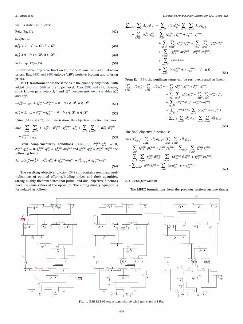
Fig. 1. IEEE RTS-96 test system with 19 wind farms and 3 BSUs.

K. Pandžić et al. Electrical Power and Energy Systems 104 (2019) 401–413

406

single VSP owns all the BSUs in the system. However, one may expectmultiple VSP owners operating their BSUs and competing for profit,which resembles an EPEC structure. The solution of this EPEC problemis a set of equilibria, in which none of the VSPs is able to increase itsrevenue unilaterally by changing the offering/bidding quantities of itsBSUs. To solve the proposed EPEC we use the diagonalization algo-rithm, which is implemented by sequentially solving one MPEC at atime. That is, MPECs are solved one by one, considering fixed the de-cisions of the remaining MPECs. Once all VSP’s MPECs are solved, thesolving cycle restarts as many times as needed for the decision variablesof each MPEC to stabilize. Additional information on the use andproperties of the diagonalization procedure are available in [53].

The upper-level problem schedules the BSUs to maximize the profitof the current VSP, while the lower-level problem considers both thecurrent VSP and all other VSPs with their decisions fixed from theprevious iteration. In the price-quantity environment, every BSU has anincentive to lower the offering price in order to seize the market. Theprice lowering continues until reaching the marginal costs. Therefore,we use the quantity-only model where BSUs offer at zero price and bidat market cap price.

To make distinction between BSU ownership, a new set ΩJ is added.Objective function (46) and upper-level constraints (17) are valid∀ ∈h ΩH(J), i.e., for all h pertaining to owner j. The equations from thelower-level problem consider all the BSUs participating in the market,i.e., they constrain all ∈h ΩH.

3. Case study

The proposed model is tested on IEEE RTS-96 supplemented with 19wind farms (see Fig. 1), whose output throughout the representativeweek is shown in Fig. 2. The representative week is obtained from theannual data available in [54] using the fast-forward scenario reductionalgorithm described in [55]. During this week, the overall system loadranges from 3900MW to 8100MW, while the daily consumption rangesfrom 121 GWh to 161 GWh. Available wind power ranges from 1 to 3%in some hours of days 2 and 5, and all the way to over 100% of the loadduring the night hours between days 1–2 and 6–7. Three BSUs are lo-cated at buses 106, 117 and 220, which are identified as attractivelocations for performing arbitrage [20]. Their energy capacity in thiscase study is 100, 250 or 500 MWh each, which is almost negligible interms of daily consumption during the low available wind power, butcan be significant during the days in which the available wind power iscomparable to the overall load.

The presented case study is implemented in GAMS 24.5 and solvedusing CPLEX 12.6. The optimality gap is set to 0,5%.

3.1. Effects of optimization time horizon

An important issue when optimizing a merchant BSU is the opti-mization time horizon. Here, we analyze if it is sufficient to consideronly one day at a time or if a longer look-ahead period may bring higherprofit. To examine this, we analyze profits of a single 250 MWh BSUlocated at bus 117. Table 1 compares its profits using one-day look-ahead, two-days look-ahead, and a week look-ahead scheduling horizon(all three cases consider day-ahead market where market bids and of-fers are submitted one day in advance). The results show that the loss ofprofit when looking only a day ahead, without trying to forecast theprices after this day, is 32% as opposed to the case when the prices areaccurately forecasted for one week ahead. On the other hand, the two-day look-ahead horizon performs as well as the one week look-aheadhorizon. This is because the duration of storage is one hour, so there isno long-term storing of energy. This indicates that a merchant-ownedBSU should forecast market outcomes for two days in advance, and notonly for the following day. Longer scheduling horizon allows a BSU toprecharge and/or preserve the stored energy from the previousday, thus gaining higher overall profit. However, although a BSU

significantly benefits from longer scheduling horizons, it is difficult toaccurately predict load levels and market clearing outcomes a weekahead. On the other hand, the two day look-ahead scheduling providesa good balance between uncertainty related to market outcomes andoptimal charging/discharging decisions. For this reason, in the re-maining subsections of the case study we use a 48-h ahead scheduling,apply the results for the first 24 h, which is the day-ahead markethorizon, and discard the last 24 h. After that, we move to the next dayand perform optimization for the second and the third day, discardingthe results for the third day, and so on.

3.2. Impact of BSU capacity on revenue

Fig. 3 shows charging/discharging schedules, states of energy andLMP profiles of three BSUs with 100MW capacity consisting a VSP. Atthe beginning of the week the BSUs were empty, while their states ofenergy transfer from one day to another is based on the state of energyat hour 24 of each optimization. The BSUs are connected to buses 106,117 and 220 and their charging and discharging capacity is set to 1C,i.e. they can fully charge or discharge within one hour.

During the first five days all three BSUs behave in a similar wayperforming one full charging/discharging cycle a day. The only ex-ception is the BSU at bus 117, which performs an additional cycle rightat the beginning of the first day. Generally, all the BSUs charge duringthe low-price periods and discharge during the high-price periods.However, the charging and discharging volumes are rarely 100MW,which indicates that higher volumes would have negative impact onLMPs. On day 6, the BSUs at buses 106 and 117 are idle as they can nottake advantage of the volatile prices. Namely, the LMPs decreasethroughout the day 6 and there is no opportunity for performing acharging/discharging cycle for these two BSUs. On the other hand, firmand more volatile LMPs at bus 220 allow this BSU one half and one fullcycle during day 6. The last day is abundant with wind power and LMPsare extremely low. Regardless, the BSUs at buses 106 and 220 manageto perform two full cycles, while the BSU at bus 117 performs a singlecycle. The results in Fig. 3 also indicate that the BSUs have differentstate of energy at the end of each day. For instance, the BSU at bus 106is fully charged at the end of the first day and fully discharged at theend of the second day. This confirms the importance of the two daylook-ahead optimization horizon.

Daily profit of each BSU is provided in Table 2. The highest overallprofit is obtained for the BSU at bus 220. However, it is interesting toanalyze the daily distribution of the profits. The most profitable daysare days 2 and 4. Day 2 is profitable because the BSUs fully charge inthe last hour of the first day and manage to discharge at high prices

Fig. 2. Available output of 19 wind farms within the IEEE-RTS 96 during therepresentative week [54].

K. Pandžić et al. Electrical Power and Energy Systems 104 (2019) 401–413

407

during the second day (around $25). The fourth day is also profitablebecause the BSUs are charged at the end of day 3 and beginning of day4 at zero price and then discharged in the afternoon of day 4 at around$25. In day 1, the BSU at bus 117 is most profitable due to an additional

cycle in the first few hours. Despite the similar state of energy curveduring day 1, the BSU at bus 220 is less profitable than the one at bus106 because it charges at higher cost.

Fig. 4 shows charging/discharging schedules, states of energy and

Table 1Storage profit depending on the optimization horizon, $.

Day ahead Two days ahead Week ahead

Day 1 1266 1209 1209Day 2 680 5619 5619Day 3 470 470 470Day 4 5567 5567 5568Day 5 486 481 482Day 6 486 587 597Day 7 1644 1642 1642Total 10,600 15,576 15,587

(a) BSU at bus 106

(b) BSU at bus 117

(c) BSU at bus 220

Fig. 3. VSP charging/discharging schedules, states of energy and LMP profilesfor 100 MWh BSU capacity.

Table 2Daily individual BSU profits for 100 MWh capacity, $ (%).

Bus 106 Bus 117 Bus 220 Total

Day 1 641 1287 386 2315Day 2 2255 2228 2250 6733Day 3 188 150 188 526Day 4 2128 2227 2227 6852Day 5 188 194 191 573Day 6 0 0 688 688Day 7 694 639 1044 2377

Total 6094 6725 6974 19,794

(a) BSU at bus 106

(b) BSU at bus 117

(c) BSU at bus 220

Fig. 4. VSP charging/discharging schedules, states of energy and LMP profilesfor 250MWh BSU capacity.

K. Pandžić et al. Electrical Power and Energy Systems 104 (2019) 401–413

408

LMP profiles for 250 MWh capacity BSUs. The charging/dischargingschedules are similar to the ones for 100 MWh capacity BSUs, withsome slight differences. The BSU at bus 106 is not fully charged duringthe first day in order to preserve the fairly low LMPs. Also, since itrequires more energy to fully charge at the end of the first day, it partlycharges at higher prices, thus resulting in lower daily profit (compare inTables 2 and 3). Also, it performs only two cycles during day 7, but thedaily profit is increased due to higher energy volume traded in themarket. The schedule of the BSU at bus 117 does not change much, butone can note a small negative profit in day 3. This is a result of thecharging process at the end of the day needed to achieve high profit inday 4. The 250 MWh BSU at bus 220 is scheduled with an extremelyshallow cycle during the first day, as opposed to the full cycle for the100 MWh BSU capacity. This is the result of congestion between theBSUs at buses 117 and 220. Higher charging quantity of the BSU at bus220 would incur higher LMP at bus 117. This situation clearly depictsthe joint coordination of the three BSUs within a VSP with the goal ofmaximizing profit for the entire VSP and not a single BSU. It is alsoworth noting that, as opposed to the 100 MWh BSUs, the 250 MWhBSUs never charge nor discharge at maximum rate since this wouldcause undesired changes in LMPs.

Profit of the BSU at bus 117 in Table 1 is higher than the one inTable 3 because the BSUs at buses 106 and 220 are not considered inTable 1. This indicates that existence of additional BSUs reduced thevalue of a BSU in the system.

BSU charging/discharging schedules, states of energy and LMPprofiles for 500 MWh capacity BSUs are shown in Fig. 5. As opposed tothe 100MWh and 250MWh cases, the BSU at bus 106 does not performa charging/discharging cycle during the first day. Instead, it charges tofull capacity and preserves the energy for the second day, when theprices are much higher. The result of this schedule is negative profit ofthis BSU on Day 1, which is followed by an $8,994 profit in the secondday, as shown in Table 4. The BSU connected to bus 117 performs areduced cycle, i.e. it does not fully charge, during the first day, but theremaining days of the week follow similar schedules as in case of100MWh and 250MWh BSU capacities. The BSU connected to bus 220also is also scheduled very similar as in the 250 MWh case, but withreduced charging cycle during the day 6. Table 4 indicates huge dif-ferences in profits for individual days. The most profitable days for theVSP are days 2 and 4. This is a direct outcome of the wind profile inFig. 2, where day 1 is rich with wind energy, which is charged to theVSP and injected into the system during day 2, which has very low windoutput and, consequently, high LMPs. Similarly, the late hours of day 3and early hours of day 4 are abundant in wind output, which is stored inthe VSP and discharged in the second half of day 4 at high prices.During day 6, the BSUs at buses 106 and 117 are idle and their profit inthat day is zero. This is a direct result of the increasing wind throughoutthe day, which results in almost monotonically reducing LMPsthroughout the day. Since the final LMPs in day 6 at most buses is zero,there are no arbitrage opportunities for the BSUs at buses 106 and 117.

A comparison of the total VSP profit for different BSU capacities(Tables 2–4) indicates the saturation of profit as the BSU capacity in-creases. Specifically, the overall VSP profit for 250MWh installed BSUcapacity is 2.17 times higher than in the case of 100MWh capacity,while the overall profit for 500MWh BSUs is only 3.84 times higherthan in the case of 100 MWh BSUs.

3.3. Analysis of VSP offering and bidding prices

When a BSU is charging, it is adding up to the total system load. As aresult, its purchase bid may drive the LMPs up resulting in higherpurchasing price of electricity. Similarly, when discharging, BSU acts asa generation resource and may reduce the LMP, resulting in a lowerselling price. For this reason, the BSU offering and bidding prices, i.e.variables αt h,

dis and αt h,ch from the model presented in Section 2.3, are for

the most part identical to the expected LMPs.

To maximize its profit, VSP bids and offers quantities that do notalter the LMPs significantly. In Figs. 6–8, the VSP charging bids aremarked with red circles and discharging offers with blue circles. All thebids are accepted and the circles basically represent the time periods inwhich a BSU was charged (red circles) or discharged (blue circles).

The LMPs with and without BSUs in Figs. 6–8 indicate very low changesin LMPs due to BSU actions. In most graphs, the blue line, representing theLMPs when there are no BSUs in the system, is behind the red line, whichshows the LMPs when BSUs are participating in the market. The increasedLMPs appear around hour 72 for 100 and 250MWh capacities of the BSU atbus 106 (Figs. 6a and b). The 250MWh BSU at bus 117 even manages toperform a small charging/discharging cycle around hour 72 (Fig. 7b).However, an interesting situation occurs at the end of the third day for the100MWh BSU at bus 117. This BSU actually discharges at zero price andthen charges in the next two hours, again at zero price. The dischargedquantity is actually quite high, around 25MWh (see Fig. 3b). Although thissmall charging/discharging cycle has no effect on the objective function,since both the charging and discharging prices are zero, this should beavoided as it unnecessary increases degradation of the BSU. This can beavoided by implementing a degradation model, e.g. [56]. A reduction of theLMPs due to BSU discharging is noticed at the end of the last day, e.g.Figs. 6b, 8a and 8b.

3.4. Competition between the VSPs using EPEC

In the previous subsections of the case study, all three BSUs wereowned and operated by a single VSP, which means they offer and bid inthe market in a coordinated manner. Here, we compare the results ofthe coordinated scheduling of the three 100MWh BSUs under a singleVSP (Table 2) to a setting in which each of the BSUs has a differentowner. In this case, all three BSUs, now each of them being a VSP of itsown, maximize their profit independently of the other two VSPs andcompete among each other.

The competitive price setting optimization model is a classicalBertrand model [57]. In a Bertrand pricing game, a Nash equilibrium 1

is found when all competitors bid at the same price, which is equal tothe marginal cost. If the price set by the competitors is the same buthigher than the marginal cost, there will be an incentive for the com-petitors to lower their prices and seize the market. Therefore, the onlyequilibrium in which none of the competitors will be willing to deviateis when the price equals competitors’ marginal cost. When optimizedsimultaneously, BSUs offer at a price that is usually higher than theirmarginal cost which is assumed to be zero. In the EPEC model, offeringat a price above marginal cost would leave a competitor VSP an in-centive to lower its offering price to seize the market. The process oflowering the price to seize the market would repeat until all the VSPsoffer at their marginal cost.

Table 3Daily individual BSU profits for 250MWh capacity, $ (%).

Bus 106 Bus 117 Bus 220 Total

Day 1 459 1309 18 1786Day 2 5568 5480 5596 16,644Day 3 7 −28 463 442Day 4 5189 5566 5473 16,228Day 5 603 456 467 1527Day 6 0 0 923 923Day 7 1648 1582 2134 5364

Total 13,474 14,366 15,075 42,914

1 Nash equilibrium is a game theory solution concept of a non-cooperativegame that involves several players. Nash equilibrium is a point in which anychange to a player’s strategy does not result in additional benefit. Detailed in-formation are available in[58].

K. Pandžić et al. Electrical Power and Energy Systems 104 (2019) 401–413

409

Since the BSUs’ marginal operating cost is zero, in EPEC model weuse the quantity-only offering model from [59] with offering price set to$0 and bidding price to the market cap. The diagonalization algorithmused to solve the EPEC is implemented by sequentially solving an MPEC

for each VSP considering fixed the decisions of the remaining VSPs.When using the diagonalization algorithm, the profit that a BSU (VSP)makes greatly depends on its precedence to set the offering/biddingquantities. The aim of this analysis is to characterize possible equilibria.It is important to emphasize that the presented diagonalization proce-dure does not reflect actual mechanics of the VSP competition, as allVSPs submit their offer simultaneously. Instead, this analysis aims atcharacterizing possible equilibria that can occur in this competition andfind a range of possible VSP profits when competing with other VSPs.

Profits of individual 100MWh VSPs for all six possible equilibriumoutcomes are listed in Table 5. For example, if the VSP connected to bus106 is scheduled first, its profit is $6705 or $6802, depending on thescheduling sequence of the other two VSPs. These two profits are higherthan the profits where the BSU at bus 106 is a part of the bigger VSP($6094), but the profit of the other two VSPs are decreased. The overallprofit of the three VSPs is $18,910 and $18,992, depending on thescheduling sequence of the other two VSPs, which is over 4% lowerthan in case of the coordinated approach of all three BSUs under asingle VSP (see Table 2). Similar conclusions are derived for the othertwo VSPs. Regardless of the sequence of the VSP scheduling, theiroverall profit is lower (up to 7%) than if their actions are coordinatedunder a single VSP. Considering that all market participants submittheir offers and bids individually and independently and that themarket outcome is known only after the market operator performs theclearing procedure, it is important to understand the meaning of theprofits listed in Table 5. The profits where a specific VSP solves itsMPEC first in the EPEC procedure represent an upper bound on itspossible profit in the market, while the lower profits indicate the lowerbound of the possible VSP profit. The actual VSP profit depends on itsquality of scheduling and accurate consideration of the other VSPs’decision-making processes.

3.5. Neglecting other VSPs at the bidding stage

In order to evaluate the importance of considering other VSPs at thebidding stage, we perform a simulation where each of the three VSPs(each VSP owning a single BSU) derives its optimal bidding strategy bycompletely neglecting other VSPs and their bidding strategies. This isachieved by using the MPEC from Section 2.2 and ignoring the BSUsowned by other VSPs. The obtained VSP bidding strategies are thenused to simulate actual market clearing represented by constraints(5)–(15). The resulting LMPs, which may be different than those ex-pected at the scheduling stage, are then used to determine the actualVSP profits.

Table 6 shows the reduction of profit as compared to Table 2. For100MWh VSPs, the overall weekly profit of the VSP at bus 106 reducesfrom $6094 to only $270. This is mainly because of a huge spike in LMPat this bus at hour 24 (see Fig. 9a) caused by neglecting the other VSPsin the system at the bidding stage. Actually, at hour 24 the LMP at allthree VSP buses is zero and all three VSPs decided to charge at fullcapacity. This caused an extremely high LMP at bus 106 (over $60) andcaused great monetary losses to the VSP at bus 106. The VSP losses onday 2 are negligible, while on day 3 the VSP at bus 117 actually hadhigher profit due to reduced profit for the VSPs at buses 106 and 220(the overall profit of all the VSPs on day 3 is reduced by 35%). Theprofit on days 4–6 is only slightly reduced, while the overall profit onday 7 is reduced by 26%. In total, the VSPs made 34% lower profit ascompared to their coordinated bidding presented in Table 2. The resultsof the simulations indicate that with the increasing energy storage ca-pacity in the power system, it is necessary to anticipate the competitors’decisions. This might be harder task than anticipating the strategicdecisions of the generators as the BSUs do not have (or have very low)operating costs and throughout the day may bid different quantities atdifferent prices. The generators are making profit as long as the LMP ishigher than their marginal cost. On the other hand, BSUs are makingprofit if their selling price is higher than their purchasing price plus the

(a) BSU at bus 106

(b) BSU at bus 117

(c) BSU at bus 220

Fig. 5. VSP charging/discharging schedules, states of energy and LMP profilesfor 500MWh BSU capacity.

Table 4Daily individual BSU profits for 500MWh capacity, $ (%).

Bus 106 Bus 117 Bus 220 Total

Day 1 −2891 857 −346 −2380Day 2 8994 11,133 8179 28,306Day 3 1764 −855 3725 4633Day 4 7546 10,179 10,756 28,480Day 5 3150 1801 886 5837Day 6 0 0 932 932Day 7 3229 3118 3840 10,187

Total 31,792 26,233 27,970 75,995

K. Pandžić et al. Electrical Power and Energy Systems 104 (2019) 401–413

410

(a) 100 MWh capacity (b) 250 MWh capacity

(c) 500 MWh capacity

Fig. 6. BSU at bus 106 offering strategy and LMPs.

(a) 100 MWh capacity (b) 250 MWh capacity

(c) 500 MWh capacity

Fig. 7. BSU at bus 117 offering strategy and LMPs.

(a) 100 MWh capacity (b) 250 MWh capacity

(c) 500 MWh capacity

Fig. 8. BSU at bus 220 offering strategy and LMPs.

K. Pandžić et al. Electrical Power and Energy Systems 104 (2019) 401–413

411

cycle efficiency. This means that the outcome of the quantity-only of-fering model with selling price set to zero and purchasing price atmarket cap can be significantly different than anticipated. Therefore,the VSPs should consider using the price-and-quantity offering model toprotect against the undesired market outcomes.

4. Conclusions

This paper exploits MPEC and EPEC structure to evaluate the profitopportunities of BSUs in the day-ahead energy market. The followingconclusions are derived:

1. Due to energy preservation and precharge abilities, a BSU shouldforecast market outcomes for two days in advance in order to

maximize its overall profits. However, forecasting market prices,especially as a price taker in a system with high integration of windenergy might be a difficult task and two-days scheduling horizonmight not be optimal in for specific cases. Therefore, the quality offorecasting market prices will determine the look-ahead horizon forenergy storage.

2. BSUs behave in a way to minimize their impact on LMPs. For thisreason, they may discharge/charge at hours whose LMPs are nothighest/lowest. As a consequence, in the analyzed case study theyusually charge and discharge during multiple hours (despite the 1 hduration of storage) in order to not affect the LMPs and reduce theirprofits.

3. The characteristics of the BSUs from the case study are suitable forperforming daily arbitrage. However, in order to maximize theirprofit, the BSUs might miss their daily charging/discharging cycle inorder to charge at very low price and preserve the energy for dis-charging at high prices in the following day.

4. Comparison of the MPEC and EPEC settings allows BSUs to reach anequilibrium encompassing their individual maximum revenue tar-gets.

5. Coordinated BSU strategy in the day-ahead market results in sig-nificantly higher profits as compared to the uncoordinated EPECapproach.

6. In the uncoordinated approach, BSU profits are highly dependent onthe BSU scheduling sequence, which means that there are manyequilibria with uneven distribution of profits.

7. Discarding other storage facilities at the day–ahead schedulingphase may result in a huge reduction of profit or even incur a loss fora VSP. This is because only a slightly higher charging/discharginglevel may cause severe upward/downward price spikes.

The running time for the 48-h horizon in all the simulations is below2min, which makes it useful for medium-scale power systems.Generator offering curves may be derived using the historical marketdata and inverse optimization techniques. However, the impact of un-certainty of wind generation and load levels remains to be investigatedin future research. This would allow assessing the impact of forecastingerrors and enable an additional revenue stream for the VSPs from theintraday and/or balancing markets.

Table 5Profit of 100MWh VSPs at buses 106, 117 and 220 for different VSP schedulingsequences, $.

First VSP 106 117 220

Second VSP 117 220 106 220 106 117

106 6705 6802 5688 5204 55,547 5002117 6120 5829 7149 7212 5976 6120220 6085 6361 6118 6409 7407 7292

Total 18,910 18,992 18,955 18,825 18,930 18,414

Table 6Daily individual BSU profits for 100 MWh capacity when neglecting other VSPsat the scheduling stage, $ (%).

Bus 106 Bus 117 Bus 220 Total

Day 1 −4993 (−∞%) 1098 (−15%) 275 (−29%) −3620 (−∞%)Day 2 2228 (−1%) 2228 (0%) 2228 (−1%) 6683 (−1%)Day 3 77 (−59%) 188 (26%) 79 (−58%) 344 (−35%)Day 4 2128 (0%) 2227 (0%) 2227 (0%) 6581 (0%)Day 5 188 (0%) 184 (−5%) 191 (0%) 564 (−2%)Day 6 0 (0%) 0 (0%) 677 (−2%) 677 (−2%)Day 7 642 (−8%) 487 (−24%) 635 (−39%) 1764 (−26%)

Total 270 (−96%) 6412 (−5%) 6311 (−10%) 12993 (−34%)

(a) Bus 106 (b) Bus 117

(c) Bus 220

Fig. 9. Difference in LMPs after the actual market clearing when the VSPs neglect and when they consider other VSPs at the scheduling stage.

K. Pandžić et al. Electrical Power and Energy Systems 104 (2019) 401–413

412

Acknowledgement

This work has been supported by the Croatian Science Foundationand the Croatian TSO (HOPS) under the project Smart Integration ofRENewables – SIREN (I-2583-2015) and through European Union’sHorizon 2020 research and innovation program under projectCROSSBOW – CROSS BOrder management of variable renewable en-ergies and storage units enabling a transnational Wholesale market(Grant No. 773430).

References

[1] Ela E, Milligan M, Kirby B. Operating Reserves and Variable Generation, TechnicalReport – National Renewable Energy Laboratory; 2011.

[2] Guizzi GL, Iacovella L, Manno M. Intermittent non-dispatchable renewable gen-eration and reserve requirements: historical analysis and preliminary evaluations onthe italian electric grid. Energy Procedia 2015;81. 339–334.

[3] Rasmussen MG, Andersen GB, Greiner M. Storage and balancing synergies in a fullyor highly renewable pan-european power system. Energy Policy2012;51(2):642–51.

[4] Energinet [Online]. Available at:energinet.dk/EN/El/Nyheder/Sider/Danskvindstroem-slaar-igen-rekord-42-procent.aspx.

[5] European Association for Storage of Energy (EASE) and European Energy ResearchAlliance (EERA), European Energy Storage Technology Development Roadmap to-wards 2030. [Online]. Available at:www.eera-set.eu/wp-content/uploads/148885-EASE-recommendations-Roadmap-04.pdf.

[6] Pandžić K, Pandžić H, Kuzle I. Coordination of Regulated and Merchant EnergyStorage Investments. In IEEE Transactions on Sustainable Energy, early access.

[7] McPherson M, Tahseen S. Deploying storage assets to facilitate variable renewableenergy integration: the impacts of grid flexibility, renewable penetration, andmarket structure. Energy 2018;145:856–70.

[8] International Energy Agency. Energy Technology Perspectives 2016 – TowardsSustainable Urban Energy Systems.

[9] Terna storage overview. [Online]. Available at:https://www.terna.it/en-gb/sistemaelettrico/progettipilotadiaccumulo.aspx.

[10] DoE Global Energy Storage Database. [Online]. Available at:https://www.energystorageexchange.org/projects.

[11] NGK Insulators Ltd. [Online]. Available at:https://www.ngk.co.jp/nas/specs/.[12] Battery Technology Charges Ahead [Online]. Available:www.mckinsey.com/

insights/energyresourcesmaterials/batterytechnologychargesahead.[13] Beaudin M, Zareipour H, Schellenberglabe A, Rosehart W. Energy storage for mi-

tigating the variability of renewable electricity sources: An updated review. EnergySustain Dev 2010;14(4):302–14.

[14] Yang Y, Li H, Aichorn A, Zheng J, Greenleaf M. Sizing strategy of distributed batterystorage system with high penetration of photovoltaic for voltage regulation andpeak load shaving. IEEE Trans Smart Grid March 2014;5(2):982–91.

[15] Yau T, Walker LN, Graham HL, Gupta A, Raithel R. Effects of battery storage deviceson power system dispatch. IEEE Trans Power Apparatus Syst Jan. 1981;PAS100(1):375–83.

[16] Su HI, Gamal AE. Modeling and analysis of the role of fast-response energy storagein the smart grid. In: Proc. 49th Annual Allerton Conference on Communication,Control, and Computing (Allerton), Monticello, IL; 2011. p. 719–26.

[17] Denholm P, Sioshansi R. The value of compressed air energy storage with wind intransmission-constrained electric power systems. Energy Policy May2009;37(8):3149–58.

[18] Mokrian P, Stephen M. A Stochastic Programming Framework for the Valuation ofElectricity Storage. [Online]. Available atwww.iaee.org/en/students/bestpapers/PedramMokrian.pdf.

[19] U.S. DoE. Grid Energy Storage. [Online]. Available at:energy.gov/sites/prod/files/2014/09/f18/Grid%20Energy%20Storage%20December%202013.pdf.

[20] Pandžić H, Wang Y, Qiu T, Kirschen D. Near-optimal method for siting and sizing ofdistributed storage in a transmission network. IEEE Trans Power Syst Sept.2015;30(5):2288–300.

[21] Hartwig K, Kockar I. Impact of strategic behavior and ownership of energy storageon provision of flexibility. IEEE Trans Sustain Energy April 2016;7(2):744–54.

[22] Pang JS, Fukushima M. Quasi-variational inequalities, generalized Nash equilibria,and multi-leader-follower games. CMS 2005;2(1):21–56.

[23] Hobbs BF, Metzler CB, Pang JS. Strategic gaming analysis for electric power sys-tems: an MPEC approach. IEEE Trans Power Syst May 2000;15(2):638–45.

[24] Chen Y, Hobbs BF, Leyffer S, Munson TS. Leader-follower Equilibira for electricpower and NOx allowances markets. CMS 2006;3(4):307–30.

[25] Ralph D, Smeers Y. EPECs as models for electricity markets, in Proceedings of PowerSystems Conference and Exposition, Atlanta USA; 2006.

[26] Ruiz C, Conejo AJ, Smeers Y. Equilibria in an oligopolistic electricity pool withstepwise offer curves. IEEE Trans Power Syst May 2012;27(2):752–61.

[27] Pandžić H, Conejo A, Kuzle I. An EPEC approach to the yearly maintenance sche-duling of generating units. IEEE Trans Power Syst 2013;28(2):922–30.

[28] Dvorkin Y, Fernndez-Blanco R, Kirschen DS, Pandžić H, Watson JP, Silva-MonroyCA. Ensuring profitability of energy storage. IEEE Trans Power Syst Jan.2017;32(1):611–23.

[29] Johnson JX, De Kleine R, Keoleian GA. Assessment of energy storage for trans-mission-constrained wind. Appl Energy Apr. 2014;124:377–88.

[30] Wogrin S, Galbally D, Reneses J. Optimizing storage operations in medium- andlong-term power system models. IEEE Trans Power Syst Sept. 2015;31(4):3129–38.

[31] Muche T. Optimal operation and forecasting policy for pump storage plants in day-ahead markets. Appl Energy Jan. 2014;113:1089–99.

[32] Wogrin S, Gayme DF. Optimizing storage siting, sizing, and technology portfolios intransmission-constrained networks. IEEE Trans Power Syst Nov.2015;30(6):3304–13.

[33] O’Dwyer C, Flynn D. Using energy storage to manage high net load variability atsub-hourly time-scales. IEEE Trans Power Syst July 2015;30(4):2139–48.

[34] Varkani AK, Daraeepour A, Monsef H. A new self-scheduling strategy for integratedoperation of wind and pumped-storage power plants in power markets. Appl EnergyDec. 2011;88(12):5002–12.

[35] Pandžić H, Kuzle I, Capuder T. Virtual power plant mid-term dispatch optimization.Appl Energy Jan. 2013;101(1):134–41.

[36] Dicorato M, Forte G, Pisani M, Trovato M. Planning and operating combined wind-storage system in electricity market. IEEE Trans Power Syst April2012;3(2):209–17.

[37] Akhavan-Hejazi H, Mohsenian-Rad H. Optimal operation of independent storagesystems in energy and reserve markets with high wind penetration. IEEE TransSmart Grid March 2014;5(2):1088–97.

[38] Berrada A, Loudiyi K, Zorkani I. Valuation of energy storage in energy and reg-ulation markets. Energy Nov 2016;115:1109–18.

[39] Cho J, Kleit AN. Energy storage systems in energy and ancillary markets: a back-wards induction approach. Appl Energy June 2015;147:176–83.

[40] McConnell D, Forcey T, Sandiford M. Estimating the value of electricity storage inan energy-only wholesale market. Appl Energy Dec. 2015;159:422–32.

[41] Zafirakis D, Chalvatzis KJ, Baiocchi G, Daskalakis G. The value of arbitrage forenergy storage: evidence from European electricity markets. Appl Energy Dec.2016;184:971–86.

[42] Yu N, Foggo B. Stochastic valuation of energy storage in wholesale power markets.Energy Econ May 2017;64:177–85.

[43] Mohsenian-Rad H. Coordinated price-maker operation of large energy storage unitsin nodal energy markets. IEEE Trans Power Syst Jan. 2016;31(1):786–97.

[44] Nasrolahpour E, Kazempour J, Zareipour H, Rosehart WD. Impacts of ramping in-flexibility of conventional generators on strategic operation of energy storage fa-cilities. IEEE Trans Smart Grid 2016(99). pp. 1–1.

[45] Yujian Ye, Papadaskalopoulos D, Strbac G. An MPEC approach for analysing theimpact of energy storage in imperfect electricity markets. In: 2016 13thInternational Conference on the European Energy Market (EEM), Porto; 2016.p. 1–5.

[46] Zou P, Chen Q, Xia Q, He G, Kang C, Conejo AJ. Pool equilibria including strategicstorage. Appl Energy May 2016;177:260–70.

[47] Shahmohammadi A, Sioshansi R, Conejo AJ, Afsharnia S. Market equilibria andinteractions between strategic generation, wind, and storage. Appl Energy2018;220:876–92.

[48] Sioshansi R. When energy storage reduces social welfare. Energy Econ Jan2014;41:106–16.

[49] Schill W-P, Kemfert C. Modeling strategic electricity storage: the case of pumpedhydro storage in Germany. Energy J 2011;32(3):59–87.

[50] Ruiz C, Conejo AJ, Bertsimas DJ. Revealing rival marginal offer prices via inverseoptimization. IEEE Trans Power Syst Aug. 2013;28(3):3056–64.

[51] Gabriel SA, Conejo AJ, Fuller JD, Hobbs BF, Ruiz C. Complementarity modeling inenergy markets. Springer; 2013.

[52] Fortuny-Amat J, McCarl B. A representation and economic interpretation of a twolevel programming problem. J Oper Res Soc Sept. 1981;32(9):783–92.

[53] Su Che-Lin. Equilibrium problems with equilibrium constraints: stationarities, al-gorithms, and applications [Ph.D. thesis]. Stanford University; 2005 Availableat:https://web.stanford.edu/group/SOL/dissertations/clsu-thesis.pdf.

[54] Pandžić H, Dvorkin Y, Qiu T, Wang Y, Kirschen D. Unit Commitment underUncertainty GAMS Models, Library of the Renewable Energy Analysis Lab (REAL),University of Washington, Seattle, USA. [Online]. Available at:www.ee.washington.edu/research/real/gamscode.html.

[55] Gröwe-Kuska N, Heitsch H, Roömisch W, Scenario reduction and scenario treeconstruction for power management problems. In: Proc. IEEE Bologna PowerTechnol. Conf., Bologna, Italy; 2003.

[56] Sarker MR, Pandžić H, Sun K, Ortega-Vazquez MA. Optimal operation of aggregatedelectric vehicle charging stations coupled with energy storage. IET Gener TransmDistrib 2018;12(5):1127–36.

[57] Bertrand J. Theorie mathematique de la richesse sociale. J des Savants1883;67:499–508.

[58] Dutta PK. Strategies and games: theory and practice. Massachusetts Institute ofTechnology; 1999.

[59] Pandžić H, Kuzle I. Energy storage operation in the day-ahead electricity market. In:Proceedings of the 12th International Conference on the European Energy Market(EEM), Lisbon, Portugal; 2015. p. 1–6.

K. Pandžić et al. Electrical Power and Energy Systems 104 (2019) 401–413

413