ELECTRIC CIRCUITS

CMPE 253

DEPARTMENT OF COMPUTER ENGINEERING

LABORATORY MANUAL

ISHIK UNIVERSITY

2017-2018

1

WEEK EXPERIMENT TITLE NUMBER OF EXPERIMENT

Instructional Objective

1 No Meeting

2 Tutorial 1

3 Verification of Kirchhoff’s Laws 1

To verify Kirchhoff’s current law and Kirchhoff’s voltage law for the given circuit.

4 Resistor Networks, Millman’s and Reciprocity Theorems 2

To investigate what happens when resistors are interconnected in a circuit. To observe the effect of more than one voltage source in a network (superposition principle). To satisfy KVL and KCL for a resistive circuit.

5 Tutorial 2

6 Verification of Superposition Theorem

3 To verify the superposition theorem for the given circuit.

7 MIDTERM WEEK

8 Verification of Thevenin’s Theorem

4 To verify Thevenin’s Theorem and to find the full load current for the given circuit.

9 Verification of Norton’s Theorem 5

To verify Norton’s theorem for the given circuit.

10 Verification of Maximum Power Transfer Theory

6 To verify maximum power transfer theorem for the given circuit.

11 Tutorial 3

12 Practice of using an Oscilloscope

7

In this experiment we shall study how to use the oscilloscope to make some measurements in the lab.

13 Time Constants of RC and RL Circuits

8 To investigate the factors determining the charge and discharge time for a capacitive and inductive circuits.

14

Sinosoidal Steady State

9

This experiment demonstrates the properties of ac networks. The concept of impedance is discussed. Phasors are demonstrated through oscillograms.

15 FINAL EXAMS

16 FINAL EXAMS

2

LAB EQUIPMENTS

Function Generator

A function generator is a piece of electronic test equipment or software used to generate different types

of electrical waveforms over a wide range of frequencies. Some of the most common waveforms

produced by the function generator are the sine, square, triangular and sawtooth shapes. These

waveforms can be either repetitive or single-shot (which requires an internal or external trigger source).

Integrated circuits used to generate waveforms may also be described as function generator ICs. In

addition to producing sine waves, function generators may typically produce other repetitive waveforms

including sawtooth and triangular waveforms, square waves, and pulses.

ANALOG FUNCTION GENERATOR

Oscilloscope

An oscilloscope, previously called an oscillograph and informally known as a scope or o-scope, CRO (for

cathode-ray oscilloscope), or DSO(for the more modern digital storage oscilloscope), is a type of electronic

test instrument that allows observation of constantly varying signal voltages, usually as a two-dimensional

plot of one or more signals as a function of time. Other signals (such as sound or vibration) can be

converted to voltages and displayed.

Oscilloscopes are used to observe the change of an electrical signal over time, such that voltage and time

describe a shape which is continuously graphed against a calibrated scale. The observed waveform can be

analyzed for such properties as amplitude, frequency, rise time, time interval, distortion and others.

3

DIGITAL OSCILLOSCOPE

Digital Multimeter

A multimeter or a multitester, also known as a VOM (volt-ohm-milliammeter), is an electronic measuring

instrument that combines several measurement functions in one unit. A typical multimeter can

measure voltage, current, and resistance. Analog multimeters use a microammeter with a moving pointer

to display readings. Digital multimeters have a numeric display, and may also show a graphical bar

representing the measured value. Digital multimeters are now far more common due to their cost and

precision, but analog multimeters are still preferable in some cases, for example when monitoring a

rapidly varying value.

A multimeter can be a hand-held device useful for basic fault finding and field service work, or a bench

instrument which can measure to a very high degree of accuracy. They can be used to troubleshoot

electrical problems in a wide array of industrial and household devices such as electronic equipment,

motor controls, domestic appliances, power supplies, and wiring systems.

DUAL DISPLAY DIGITAL MULTIMETER HANDHELD DIGITAL MULTIMETER

4

Power Supply

A power supply is an electronic device that supplies electric energy to an electrical load. The primary

function of a power supply is to convert one form of electrical energy to another. As a result, power

supplies are sometimes referred to as electric power converters. Some power supplies are discrete, stand-

alone devices, whereas others are built into larger devices along with their loads. Examples of the latter

include power supplies found in desktop computers and consumer electronics devices.

Every power supply must obtain the energy it supplies to its load, as well as any energy it consumes while

performing that task, from an energy source. Depending on its design, a power supply may obtain energy

from various types of energy sources, including electrical energy transmission systems, energy

storage devices such as a batteries and fuel cells, electromechanical systems such

as generators and alternators, solar power converters, or another power supply.

All power supplies have a power input, which receives energy from the energy source, and a power

output that delivers energy to the load. In most power supplies the power input and output consist

of electrical connectors or hardwired circuit connections, though some power supplies employ wireless

energy transfer in lieu of galvanic connections for the power input or output. Some power supplies have

other types of inputs and outputs as well, for functions such as external monitoring and control.

REGULATED POWER SUPPLY

PB-505 Electronics Trainer

The PB-505 is a robust electronics trainer engineered for electronics instruction and design and is ideal

for analog, digital, and microprocessor circuits. Students will learn valuable hands-on breadboarding

techniques and build a solid foundation in circuit experimentation, construction, and analysis. The PB-505

5

can be used to construct basic series and parallel circuits or the most complicated multi-stage

microcomputer circuits, incorporating new trends in industrial technology.

PB-505 ELECTRONICS TRAINER WITH BREADBOARD

Experiment No. 1 Date:

VERIFICATION OF KIRCHHOFF’S LAWS

PRE LAB QUESTIONS (Experiment No. 1)

1.Define electric energy.

2.Define electric power.

3.What is charge?

4.What is an electric network?

6

Aim: To verify Kirchhoff’s current law and Kirchhoff’s voltage law for the given circuit.

Apparatus Required:

No. Apparatus Range Quantity

1 Power supply (0-30V) 2

2 Resistors 330, 220, 1k 6

3 Ammeter (0-30mA) 3

4 Voltmeter (0-30V) 3

5 Bread Board & Jumper Wires Required

Statement:

KCL: The algebraic sum of the currents meeting at a node is equal to zero.

KVL: In any closed path / mesh, the algebraic sum of all the voltages is zero.

Precautions:

1. Voltage control knob should be kept at minimum position.

2. Current control knob of RPS should be kept at maximum position.

Procedure for KCL:

1. Give the connections as per the circuit diagram.

2. Set a particular value in the power supply.

3. Note down the corresponding ammeter reading.

4. Repeat the same for different voltages.

Procedure for KVL:

1. Give the connections as per the circuit diagram.

2. Set a particular value in the power supply.

3. Note all the voltage reading.

4. Repeat the same for different voltages.

7

Circuit – KCL

Circuit – KVL

Table 1. KCL -Theoretical Values

No. Voltage (E) Current (I) 𝑰𝟏 = 𝑰𝟐 + 𝑰𝟑

𝑰𝟏 𝑰𝟐 𝑰𝟑 Volts mA mA mA mA

1 1

2 2

3 3

4 4

5 5

8

Table 2. KCL -Practical Values

No. Voltage (E) Current (I) 𝑰𝟏 = 𝑰𝟐 + 𝑰𝟑

𝑰𝟏 𝑰𝟐 𝑰𝟑 Volts mA mA mA mA

1 1

2 2

3 3

4 4

5 5

Table 3. KVL -Theoretical Values

No. Power Supply Voltage KVL 𝑬𝟏

= 𝑽𝟏 + 𝑽𝟐 𝑬𝟏 𝑬𝟐 𝑽𝟏 𝑽𝟐 𝑽𝟑

Volts

1

2

3

4

5

Table 4. KVL -Practical Values

No. Power Supply Voltage KVL 𝑬𝟏

= 𝑽𝟏 + 𝑽𝟐 𝑬𝟏 𝑬𝟐 𝑽𝟏 𝑽𝟐 𝑽𝟑

Volts

1

2

3

4

5

9

Model Calculation:

Result: Thus Kirchhoff’s voltage and current law is verified both theoretically and practically.

POST LAB QUESTIONS (Experiment No. 1)

1. Define Ohm’s law.

2. Define Kirchhoff’s current law.

3. Define Kirchhoff’s voltage law.

10

Experiment No. 2 Date:

RESISTOR NETWORKS, MILLMAN’S AND RECIPROCITY THEOREMS

PART A: RESISTOR NETWORKS

Aim: To investigate what happens when resistors are interconnected in a circuit. To observe the effect of

more than one voltage source in a network (superposition principle). To satisfy KVL and KCL for a resistive

circuit.

Theoretical Background:

The student has to study the solution of the network from any book for electric circuits using Kirchhoff’s

law (KCL and KVL) or superposition theorem (do not concern for the superposition principle at the

moment, it will be learned later).

Apparatus Required:

No. Apparatus Range Quantity

1 Power supply (0-30V) 2

2 Resistors

0.33K, 2.2K, 1.8K,

1K, 0.47K

1

3 Ammeter (0-30mA) 1

4 Voltmeter (0-30V) 1

5 Bread Board & Jumper Wires Required

Statement:

KCL: The algebraic sum of the currents meeting at a node is equal to zero.

KVL: In any closed path / mesh, the algebraic sum of all the voltages is zero.

Precautions:

1. Voltage control knob should be kept at minimum position.

2. Current control knob of RPS should be kept at maximum position.

Procedure A:

1. Connect the circuit as shown in Figure 1.

11

Figure 1

2. Adjust the output voltage from power supply unit (PSU) to be 5 volts.

3. Using your voltmeter, measure the voltage across each resistor (Note the polarity of each voltage), then tabulate your results in Table 1.

Resistor Marked Value (KΩ) Current (mA) Voltage (Volts) Actual Value (KΩ)

R1 1.8

R2 1

R3 2.2

R4 0.33

R5 0.47

Table 1

4. Measure the current in each component using the multimeter, then tabulate your results in Table 1.

5. From the measured values of current and voltage in each branch, calculate using ohms law the

value of the resistance in each leg of the network, and copy the results in Table 1.

6. Solve the circuit using node voltage method and mesh current method, and compare the results (ignore this part).

Procedure B:

1. Connect the circuit as shown in Figure 2.

12

Figure 2

2. Switch on the PSU, measure the current in each branch of the network, this will give the currents in R1, R2, R3 and R5 respectively due to the two sources. Note both the magnitude and polarity of each current and tabulate them in Table 2.

Resistor Marked Value (KΩ) I (mA) I’ (mA) I” (mA) I’ (mA) + I” (mA)

R1 1.8

R2 1

R3 2.2

R4 0.33

R5 0.47

Table 2

3. Now disconnect the 15 V source and link the resistors R3 and R5 as shown in the circuit in Fig. 3.

Figure 3

4. Measure and tabulate the magnitude and polarity of the currents I1’, I2’, I3’, I4’ and I5’.

13

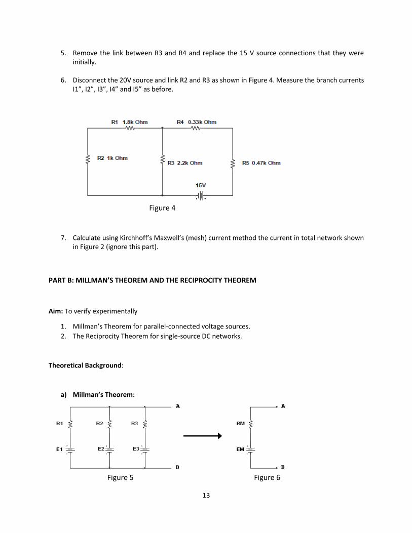
5. Remove the link between R3 and R4 and replace the 15 V source connections that they were initially.

6. Disconnect the 20V source and link R2 and R3 as shown in Figure 4. Measure the branch currents

I1”, I2”, I3”, I4” and I5” as before.

Figure 4

7. Calculate using Kirchhoff’s Maxwell’s (mesh) current method the current in total network shown in Figure 2 (ignore this part).

PART B: MILLMAN’S THEOREM AND THE RECIPROCITY THEOREM

Aim: To verify experimentally

1. Millman’s Theorem for parallel-connected voltage sources.

2. The Reciprocity Theorem for single-source DC networks.

Theoretical Background:

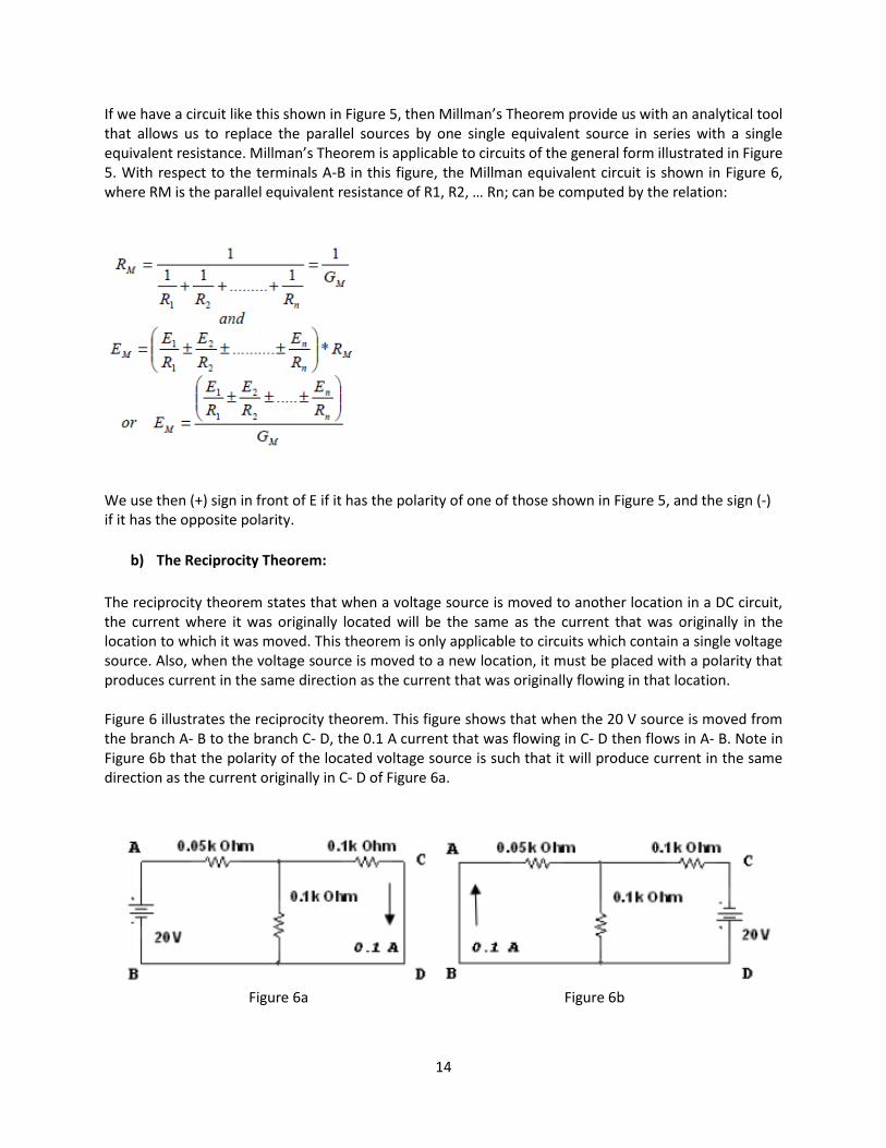
a) Millman’s Theorem:

Figure 5 Figure 6

14

If we have a circuit like this shown in Figure 5, then Millman’s Theorem provide us with an analytical tool that allows us to replace the parallel sources by one single equivalent source in series with a single equivalent resistance. Millman’s Theorem is applicable to circuits of the general form illustrated in Figure 5. With respect to the terminals A-B in this figure, the Millman equivalent circuit is shown in Figure 6, where RM is the parallel equivalent resistance of R1, R2, … Rn; can be computed by the relation:

We use then (+) sign in front of E if it has the polarity of one of those shown in Figure 5, and the sign (-) if it has the opposite polarity.

b) The Reciprocity Theorem:

The reciprocity theorem states that when a voltage source is moved to another location in a DC circuit, the current where it was originally located will be the same as the current that was originally in the location to which it was moved. This theorem is only applicable to circuits which contain a single voltage source. Also, when the voltage source is moved to a new location, it must be placed with a polarity that produces current in the same direction as the current that was originally flowing in that location. Figure 6 illustrates the reciprocity theorem. This figure shows that when the 20 V source is moved from the branch A- B to the branch C- D, the 0.1 A current that was flowing in C- D then flows in A- B. Note in Figure 6b that the polarity of the located voltage source is such that it will produce current in the same direction as the current originally in C- D of Figure 6a.

Figure 6a Figure 6b

15

Procedure C:

1. After measuring the actual resistance values of resistors used, connect the circuit shown in Figure 7, E1 and E2 are power supplies that has been set to 5V and 10V before being connected in the circuit.

Figure 7a Figure 7b

2. Measure and record the following: a) The voltage across the terminals A- B with the 1kΩ resistor connected. b) The current in the 1kΩ resistor. c) The voltage across the open-circuited terminals A- B after having removed the 1kΩ resistor. 3. Using the resistor values measured in step 1; compute the Millman equivalent voltage and resistance EM and RM. 4. Connect the circuit as shown in Figure 7b. EM and RM are the values computed in step 3. 5. Repeat step 2-b for the circuit in Figure 7b. Procedure D:

1) Connect the circuit as shown in Figure 8a

16

Figure 8a Figure 8b

2) Measure and record the currents I1, I2 and I3 flowing as shown in the figure. 3) Now connect the power supply in series with the 1.8kΩ resistor and measure the current I. See the Figure 8b, and note the polarity of the relocated power source. 4) In a similar way, relocate the power supply so that it will be in series with the 2.2kΩ and the 470Ω resistance and again measure the current I.

Experiment No. 3 Date:

VERIFICATION OF SUPERPOSITION THEOREM

PRE LAB QUESTIONS (Experiment No. 3)

1. Define active and passive elements.

2. Define an ideal voltage source.

3. Define an ideal current source.

4. What is meant by source transformation?

17

Aim: To verify the superposition theorem for the given circuit.

Apparatus Required:

No. Apparatus Range Quantity

1 Power supply (0-30V) 2

2 Ammeter (0-10mA) 1

3 Resistors 1kΩ, 330Ω, 220Ω 3

4 Bread Board - -

5 Jumper Wires - Required

Statement:

Superposition theorem states that in a linear bilateral network containing more than one source, the

current flowing through the branch is the algebraic sum of the current flowing through that branch when

sources are considered one at a time and replacing other sources by their respective internal resistances.

Precautions:

1. Voltage control knob should be kept at minimum position.

2. Current control knob of RPS should be kept at maximum position.

Procedure:

1. Give the connections as per the circuit diagram.

2. Set a particular voltage value using RPS1 and RPS2 & note down the ammeter reading.

3. Set the same voltage in Circuit I using RPS1 alone and short circuit the terminals and note the ammeter reading.

4. Set the same voltage in RPS2 alone as in Circuit I and note down the ammeter reading.

5. Verify superposition theorem.

Circuit I

18

Circuit II

Circuit III

Table 1. Theoretical Values

Regulated Power Supply (RPS) Ammeter Reading (I) mA

1 2

Circuit I 5 V 5V 𝑰 = Circuit II 5 V 0 V 𝑰′ =

Circuit III 0 V 5V 𝑰′′ =

Table 2. Practical Values

Regulated Power Supply (RPS) Ammeter Reading (I) mA

1 2

Circuit I 5 V 5V 𝑰 =

Circuit II 5 V 0 V 𝑰′ = Circuit III 0 V 5V 𝑰′′ =

19

Model Calculations:

Result: Superposition theorem have been verified theoretically and practically.

POST LAB QUESTIONS (Experiment No.3)

1. State superposition theorem.

2. What are the Steps to solve Superposition Theorem?

3. Define unilateral and bilateral elements.

4. List limitation of superposition theorem.

20

Experiment No. 4 Date:

VERIFICATION OF THEVENIN’S THEOREM

PRE LAB QUESTIONS (Experiment No. 4)

1.Define Lumped and distributed elements.

2. What is an independent source?

3. What are dependent sources?

4. Two inductors with equal value of “L” are connected in series and parallel, what are the equivalent

inductances?

5. What are the different types of dependent or controlled sources?

Aim: To verify Thevenin’s Theorem and to find the full load current for the given circuit.

Apparatus Required:

No. Apparatus Range Quantity

1 Power supply (RPS) (0-30V) 2

2 Ammeter (0-10mA) 1

3 Resistors 1kΩ, 330Ω 3,1

4 Bread Board - Required

5 DRB - 1

Statement: Any linear bilateral, active two terminal network can be replaced by an equivalent voltage

source (VTH). Thevenin’s voltage or VOC in series with looking pack resistance RTH.

21

Precautions:

1. Voltage control knob should be kept at minimum position.

2. Current control knob of RPS should be kept at maximum position.

Procedure:

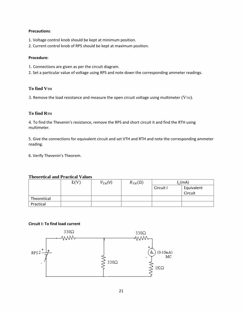
1. Connections are given as per the circuit diagram.

2. Set a particular value of voltage using RPS and note down the corresponding ammeter readings.

To find VTH

3. Remove the load resistance and measure the open circuit voltage using multimeter (VTH).

To find RTH

4. To find the Thevenin’s resistance, remove the RPS and short circuit it and find the RTH using multimeter.

5. Give the connections for equivalent circuit and set VTH and RTH and note the corresponding ammeter reading.

6. Verify Thevenin’s Theorem. Theoretical and Practical Values

E(V)

𝑉𝑇𝐻(V) 𝑅𝑇𝐻(Ω) 𝐼𝐿(mA)

Circuit I Equivalent Circuit

Theoretical

Practical

Circuit I: To find load current

22

To find VTH

To find RTH

Thevenin’s Equivalent Circuit:

23

Model Calculation:

Result: Hence the Thevenin’s Theorem is verified both practically and theoretically.

POST LAB QUESTIONS (Experiment No. 4)

1. State Thevenin’s Theorem.

2. Draw the Thevenin’s equivalent circuit.

3. What are the two quantities to be determined to apply Thevenin’s Theorem?

24

4. Write the steps to find the Thevenin’s resistance.

5. Write the steps to find the Thevenin’s voltage.

Experiment No. 5 Date:

VERIFICATION OF NORTON’S THEOREM

PRE LAB QUESTIONS (Experiment No. 5)

1. Distinguish between a branch and a node of a circuit.

2. Write down the V-I relationship of circuit elements.

3. Two capacitors with equal value of “C” are connected in series and parallel. What is the equivalent

Capacitance?

4. Write down the formula to convert a star connected network into a delta network?

5. Write down the formula to convert a delta connected network into a star network?

25

Aim: To verify Norton’s theorem for the given circuit.

Apparatus Required:

No. Apparatus Range Quantity

1 Ammeter (0-10mA) MC

(0-30mA) MC

1 1

2 Resistors 330, 1KΩ 3,1

3 RPS (Regulated Power Supply) (0-30V) 2

4 Bread Board - 1

5 Wires - Required

Statement:

Any linear, bilateral, active two terminal network can be replaced by an equivalent current source (IN) in

parallel with Norton’s resistance (RN).

Precautions:

1. Voltage control knob of RPS should be kept at minimum position.

2. Current control knob of RPS should be kept at maximum position.

Procedure:

1. Connections are given as per the circuit diagram.

2. Set a particular value in RPS and note down the ammeter readings in the original circuit.

To Find IN

3. Remove the load resistance and short circuit the terminals.

4. For the same RPS voltage note down the ammeter readings.

To Find RN

5. Remove RPS and short circuit the terminal and remove the load and note down the resistance across the two terminals.

Equivalent Circuit:

6. Set IN and RN and note down the ammeter readings.

7. Verify Norton’s theorem.

26

To find load current in circuit 1:

To find IN

To find RN

Norton’s equivalent circuit

27

Theoretical and practical values

E (Volts) IN (mA) RN (Ohm)

IL (mA)

Circuit I Equivalent Circuit

Theoretical Values

Practical Values

Model Calculations:

Result: Norton’s theorem was proved both theoretically and practically.

POST LAB QUESTIONS (Experiment No. 5)

1. State Norton’s theorem.

2. What are the Steps to solve Norton’s Theorem .

28

3. What is the load current in a Norton’s circuit?

4. What is difference between RTH and RN?

Experiment No. 6 Date:

VERIFICATION OF MAXIMUM POWER

TRANSFER THEOREM

PRE LAB QUESTIONS (Experiment No. 6)

1. Give the expression for maximum power in DC circuit. 2. Give the value of Load voltage of DC circuit under maximum power transfer condition. 3. Under what condition is the power delivered to a load maximum in DC circuit?

Aim: To verify maximum power transfer theorem for the given circuit.

Apparatus Required:

No. Apparatus Range Quantity

1 Power Source (0-30V) 1

2 Voltmeter (0-10V) MC

1

3 Resistors 1KΩ, 1.3 KΩ, 3KΩ 3

4 DRB - 1

5 Bread Board & Wires - Required

29

Statement:

In a linear, bilateral circuit the maximum power will be transferred to the load when load resistance is

equal to source resistance.

Precautions:

1. Voltage control knob of RPS should be kept at minimum position.

2. Current control knob of RPS should be kept at maximum position.

Procedure:

Circuit I 1. Connections are given as per the diagram and set a particular voltage in RPS.

2. Vary RL and note down the corresponding ammeter and voltmeter reading.

3. Repeat the procedure for different values of RL & tabulate it.

4. Calculate the power for each value of RL.

To Find VTH

5. Remove the load, and determine the open circuit voltage using multimeter (VTH) .

To Find RTH

6. Remove the load and short circuit the voltage source (RPS).

7. Find the looking back resistance (RTH) using multimeter.

Equivalent Circuit:

8. Set VTH using RPS and RTH using DRB and note down the ammeter reading.

9. Calculate the power delivered to the load (RL = RTH)

10. Verify maximum transfer theorem. Circuit I

30

To Find VTH

To Find RTH

Thevenin’s Equation Circuit

Power versus RL

31

Circuit I

No. RL (Ohm) I (mA) V(Volts) P=VI (watts)

1

2

3

4

5

6

7

8

200

400

600

800

1000

1200

1400

1600

To Find the Thevenin’s Equivalent Circuit

VTH (Volts) RTH (Ohm) IL (mA) P (miliwatts)

Theoretical

Value

Practical Value

Model Calculations:

32

Result: Thus maximum power theorem was verified both practically and theoretically. POST LAB QUESTIONS (Experiment No. 6)

1. State the maximum power transfer theorem. 2. Write some applications of the maximum transfer theorem. 3. Draw the equivalent maximum transfer theorem. 4. What are the Steps to solve Maximum power transfer theorem?

Experiment No. 7 Date:

PRACTICE OF USING AN

OSCILLOSCOPE

Aim: In this experiment we shall study how to use the oscilloscope to make some measurements in the lab. Introduction: We can use the oscilloscope to measure the frequency of a wave, the peak-to-peak value, and the rms value of voltage, also to measure the phase between two waves.

33

Apparatus Required: - Power supply unit. - Function wave generator. - Oscilloscope Theory: If a DC wave is created on the screen of the oscillator with 5V/Division on Ch1, Voltage = # of square scales of Ch1 × scale of Ch1 (5V/Div)= 2 squares × 5 Volts/Div = 10 Volts.

If two sinusoidal waves appeared on the screen, where the scale of Ch1 is 2V/Div., and the scale of Ch2 is 5v/Div. and the time base = 1 msec/Div, choose two sinusoidal waveforms with maximum voltage of 8V (Ch1) and 15 V (Ch2), then calculate the followings for both waveforms:

a. 𝑉𝑚𝑎𝑥 =? (= magnitude of the amplitude of the waveform)

b. 𝑉𝑝𝑒𝑎𝑘−𝑡𝑜−𝑝𝑒𝑎𝑘 = 𝑉𝑝−𝑝 = ? (=the magnitude from peak to peak values)

c. 𝑉𝑟𝑚𝑠 = ? (= 𝑉𝑚𝑎𝑥

√2 )

d. 𝑇(𝑝𝑒𝑟𝑖𝑜𝑑 𝑜𝑓 𝑤𝑎𝑣𝑒𝑓𝑜𝑟𝑚) =? (= the time required to complete for one full cycle)

e. 𝐹(𝑓𝑟𝑒𝑞𝑢𝑒𝑛𝑐𝑦 𝑜𝑓 𝑤𝑎𝑣𝑒𝑓𝑜𝑟𝑚) =? (= the number of full cycles per unit time or 𝐹 = 1

𝑇 )

f. 𝑃ℎ𝑎𝑠𝑒 𝑆ℎ𝑖𝑓𝑡 = ? (=the phase shift or phase angle between two waves)

*Phase shift between the two waves: If you put time base on XY mode, you will obtain a shape according to the

type of the circuit. The phase angle between two waves = sin−1 (𝑎

𝑏) .

34

Experimental Procedure:

1. Connect the circuit as shown in Figure 1.

2. Switch the Power supply, OSC. And voltmeter.

3. Change the voltage supply in steps of 2V to 10V, take readings of voltage on voltmeter and OSC.

At each step, then compare between the two results.

Figure 1

Figure Power Supply

(V)

Volt. scale # of squares Oscilloscope

reading

Voltmeter

reading

%Error

A 2

B 4

C 6

D 8

E 10

Table 1

35

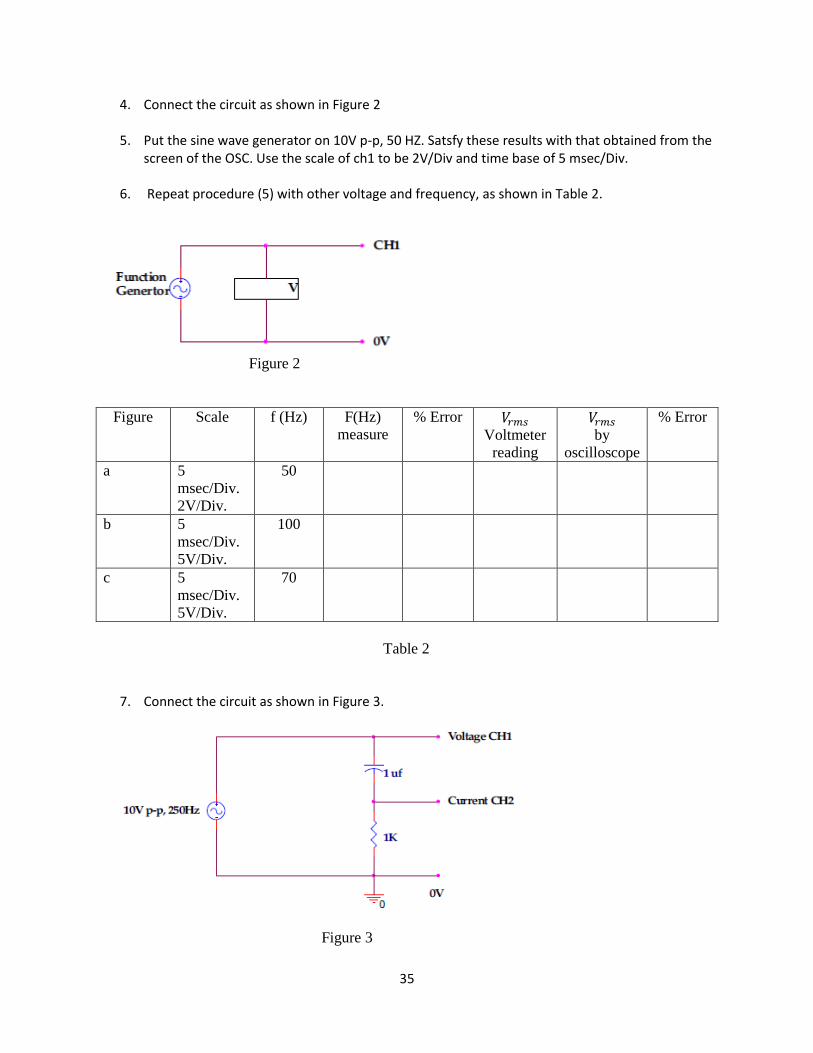
4. Connect the circuit as shown in Figure 2

5. Put the sine wave generator on 10V p-p, 50 HZ. Satsfy these results with that obtained from the screen of the OSC. Use the scale of ch1 to be 2V/Div and time base of 5 msec/Div.

6. Repeat procedure (5) with other voltage and frequency, as shown in Table 2.

Figure 2

Figure Scale f (Hz) F(Hz)

measure

% Error 𝑉𝑟𝑚𝑠 Voltmeter

reading

𝑉𝑟𝑚𝑠 by

oscilloscope

% Error

a 5

msec/Div.

2V/Div.

50

b 5

msec/Div.

5V/Div.

100

c 5

msec/Div.

5V/Div.

70

Table 2

7. Connect the circuit as shown in Figure 3.

Figure 3

36

8. Set the sine wave generator to give a 10V Peak-to-Peak at 250 Hz.

9. Set the oscilloscope as follows: a. CH1 : voltage to 2V/Div. b. CH2 : current channel to 5V/Div. Time base to 1 msec/Div.

10. Zero both traces and then observe the two waveforms on the OSC. Carefully draw the two waveforms, showing their positions with respect to each other, and the value of voltage and current. Find the phase shift between the current and the voltage in the circuit in Figure 3.

11. Set the time base at X-Y mode and obtain the value of phase shift.

12. Replace the 1 𝜇𝐹 capacitor by a 1KΩ resistor, then repeat steps 10 and 11.

Figure 4

Experiment No. 8 Date:

TIME CONSTANT OF RC AND RL

CIRCUITS

Aim: To investigate the factors determining the charge and discharge time for a capacitive and inductive circuits.

Apparatus Required:

No. Apparatus Range Quantity

1 Oscilloscope 1

2 Resistors 330Ω, 10KΩ, 0.1 KΩ 4,1

3 Function Generator 1 1

4 Bread Board - 1

5 Capacitor 100 µF 1

6 Inductor 10 mH 1

37

Theory:

The relationships of voltage and current of the capacitor in DC circuits are as follows:

After the switch is closed, the charging process begins and voltage across the capacitor rises gradually it reaches its maximum value (Vs) as shown in the right figure. The instantaneous voltage across the capacitor is

𝑉𝑐 = 𝑉𝑠 [1 − 𝑒−𝑡𝑅𝐶⁄ ]

RC is called the time constant ( τ ) of the circuit, that is τ = RC

at 𝑡 = 𝑅𝐶 = 𝜏 → 𝑉𝑐 = 𝑉𝑠[1 − 𝑒−1] = 0.63 𝑉𝑠

The time constant is the time at which the value of Vc = 0.63 Vs or 63% of Vs. The current will flow in the circuit as long as the capacitor is not completely charged. This current will be maximum at the instant the switch is closed and decreases exponentially as the charging continues.

𝑖 = 𝑐𝑑𝑉

𝑑𝑡=

𝑉𝑠

𝑅∙ 𝑒−𝑡

𝑅𝐶⁄ = 𝐼𝑚𝑎𝑥 ∙ 𝑒−𝑡𝑅𝐶⁄ , 𝑤ℎ𝑒𝑟𝑒 𝐼𝑚𝑎𝑥 =

𝑉𝑠

𝑅

38

Procedure:

I.

1) Connect the circuit as shown in Figure 1.

Figure 1

2) Connect the oscilloscope settings as follows: · Time base: 0.5 sec/div. · Ch1: 5v/div. · Ch2: 50mv/div.

3) Draw the charge and discharge waveforms of ch1 and ch2.

39

II.

1) Connect the circuit as shown in Figure 2.

Figure 2

2) Set the function generator to give a square wave of 7Hz frequency and a peak to peak voltage of 10 volts. 3) Set the oscilloscope setting as follows: · Time base: 20msec/div. · Ch1: 2v/div. · Ch2: 50mv/div. 4) For clear waveforms press the dc button of the oscilloscope. 5) Draw the charge and discharge waveforms of ch1 and ch2.

6) What is the period of the waveforms? 7) Measure the time constant from the graph.

40

8) Calculate the time constant theoretically, and then compare the results.

III.

1) Set up the circuit as shown in Figure 3. Then 33Ω resistor is to limit the maximum current reached. Then 10Ω resistor is to display the current waveform on the oscilloscope.

Figure 3

2) Adjust the wave generator to give 10 V p-p square wave at 250Hz. Set the OSC as follows: _ Time base: 0.5msec/div. _ Ch1: 2v/div. _ Ch2: 0.2v/div. 3) Take readings from the displayed current waveform and record them in Table 1. Plot the current waveform on a graph paper as large as you can. 4- Repeat step (3) for the voltage waveform. 5- Draw tangent to the current curve as its origin and calculate the slope of the curve at this point. 6- Repeat step (5) to all points and record the corresponding slope in Table 2.

Induced e.m.f. = Voltage of the inductor= Rate of change of current × L = 𝐿 ×𝝏𝒊𝑳

𝝏𝒕

*We call the constant L the inductance of the coil (inductor). 7- Plot a graph of voltage against rate of change of current and measure the slope to find L.

41

TABLE 1 TABLE 2

Experiment No. 9 Date:

Sinosoidal Steady State

Aim:

This experiment demonstrates the properties of ac networks. The concept of impedance is discussed.

Phasors are demonstrated through oscillograms.

Theory: I. AC Measurements. The RMS Value. AC instruments measure the rms (root mean square) value of the ac voltage and current. For a periodic wave form of period T, the rms value is given by:

𝑋𝑟𝑚𝑠 = √(1

𝑇∫ 𝑋2

𝑇

0

(𝑡)𝑑𝑡)

The rms of a sinusoidal quantity is given by:

𝑋𝑟𝑚𝑠 =𝑥𝑚

√2

where, 𝑥𝑚 is the amplitude of the sinusoidal quantity. The distinction between DC and AC instrumentation is important. In circuits operating in sinusoidal steady state, a dc instrument will consistently indicate zero voltage and current. The rms value of a current or voltage is, also, referred to as its effective value. This shows an equivalency between ac and dc quantities in the following sense: An AC current (voltage) produces the same power dissipation on a resistor as a DC current (voltage), which has an average (DC) value equal to the rms (effective) value of the AC current (voltage). Thus, an AC current of amplitude 1.41 A is equivalent, in the previous sense, with a DC current of average value equal 1 A. In practice, different notation is used to distinguish rms and average measurements. Thus, 10 V AC means that the rms value of the voltage measured is 10 V. While, 15 V DC means that the average value of the voltage measured is 15 V. Additional notation is available for amplitude description of AC

Time

(miliseconds)

Current

(mA)

Voltage (V)

Time

(miliseconds)

Current

(mA)

Voltage (V)

42

waveforms. Thus, 20 mA p-p (red 20 mA peak-to-peak) means that the current varies by 20 mA between two successive peaks. For a sinusoidal current this means that its amplitude is 10 mA. II. Measurements of Phasors and Impedance in the Sinusoidal Steady State. The currents and voltages of a circuit that operates in sinusoidal steady state are represented by phasors. With reference to Figure A, the impedance expresses the relation between the phasor of the terminal voltage and the phasor of the terminal current of a two-terminal RLC combination. Conversely, every passive element or two-terminal combination of passive elements possesses an impedance, which expresses the Ohm's law as follows:

= ∙ 𝐼

Figure A. Phasors and impedance in sinusoidal steady state. The magnitude of the phasor of a quantity can be measured by measuring the rms value of the quantity. The phase of the phasor can be measured using the oscilloscope. Figure B shows the oscillogram of the current and voltage at the terminals of an RLC arrangement. It is important to indicate or note the scale of the oscillogram. Notice that the oscilloscope probes measure voltage (unless a current probe is available). Appropriate scaling is required to obtain the correspondence between the oscilloscope vertical divisions and the measured current.

Figure B. The oscillogram of voltage and current.

43

For the example of Figure B, the period of the oscillations is, by reading the scale, (T/2) = 4 divisions x 2ms/division=8ms. Therefore, the period is 16 ms. This corresponds to a frequency of 62.5 Hz. The amplitude of the voltage oscillation on the oscilloscope is, by reading the scale from the reference line, 2.5 divisions. Therefore, the amplitude of the voltage is 2.5 div x 10V/div = 25 V. The rms value of the voltage is, therefore, 17.68 V. Likewise, by reading the scale, the current oscillation on the oscilloscope has an amplitude of 1.8 divisions and the actual current has an amplitude of 0.9 A. Its rms value is 0.636 A. The zero crossing displacement between voltage and current is d = 0.8 div x 2ms/div = 1.6 ms. This corresponds to a phase difference of Δφ=360° x 1.6 ms / 16 ms = 36°, with the current zero crossing leading the voltage zero crossing. From this measurements, the phasors of the voltage and current and the impedance of the RLC arrangement can be calculated. Assuming the voltage as reference:

= 25∠0𝑜𝑉

𝐼 = 0.9∠36𝑜𝐴

|| =||

|𝐼|=

25

0.9= 27.78 Ω

∠ = ∠ − ∠𝐼 = 0𝑜 − 36𝑜 = −36𝑜

Note that since the current is leading the voltage, the current's phase angle with respect to the voltage is positive. The impedance angle is the angle between current and voltage. Hence, the calculations above results in negative impedance angle. This means the RLC arrangement is capacitive. Its equivalent resistance is: R=|Z|cos(Δφ) = 22.47 Ω. Its equivalent reactance is: X=|Z|sin(Δφ) = -16.33 Ω, or 16.33 Ω Capacitive. Apparatus: - Power supply unit. - Function wave generator. - Oscilloscope Procedure: I. Measurements of Capacitive Impedance. 1. Construct the circuit of Figure 1. Set the signal generator to the sinusoidal mode. Set the frequency to 60 Hz and the amplitude to 10 V. 2. Display on the oscilloscope the current and voltage of the capacitor. 3. Vary R from 0 to 1 kΩ in increments of 100 Ω. For each value of R measure the amplitude of the voltage and current. With the voltage as reference, also measure the phase of the current. Use Table 1.

44

Figure 1. The experimental RC circuit. C= 10 μF.

Table 1. Impedance measurements in the RC circuit.

II. Measurement of Inductive Impedance. 4. (a) Construct the circuit of Figure 2. Set the source to the same values as in the previous circuit. (b) Vary R from 0 to 1 kΩ. For each value of R measure the amplitude of the voltage, the amplitude of the current, and the phase of the current to the voltage. Use Table 2.

Figure 2. The experimental RL circuit. L=100 mH.

45

Table 2. Impedance measurements in the RL circuit.

III. Measurement of the Impedance of an RLC Arrangement. 5. Construct the circuit of Figure 3. Maintain the settings of the source. Measure the magnitude of the supply voltage. Measure the magnitude and phase (with respect to the supply voltage) of the inductor current, the capacitor current and the supply current.

Figure. 3. The experimental parallel RLC circuit. R= 100 Ω, L= 100 mH, C= 10 μF.

IV. Compensation of Source Reactance. 6. (a) Construct the circuit of Figure 4 with the capacitor disconnected. Maintain the source at the settings of the previous procedure. Measure the phasors of the supply voltage and current and the phasor of the voltage across the resistor. Use the voltage across the resistor as reference. (b) Connect the capacitor. Repeat the previous measurements. Also, measure the phasor of the capacitor current.

Figure. 4. The experimental circuit to observe compensation. R= 100 Ω, L=100 mH, C=10 μ

46

V. Measurement of Parallel Resonance. 7. Construct the circuit of Figure 5. Set the supply to 1 V in the sinusoidal mode. 8. Vary slowly the frequency of the source until the amplitude of the supply current becomes minimum. For this point record the phasors of the supply voltage (reference), supply current, inductor current, and capacitor current. 9. Take the same measurements as in 8 for five frequencies below the frequency you recorded in 8. 10. Repeat 9 for five frequencies above the frequency in 8. For your measurements in 8, 9 and 10, use Table 3.

Figure. 5. The experimental setting to record resonance. R= 100 Ω, L=100 mH, C= 10 μF.

Table 3. Measurements of resonance.

Report I. A. Theoretical Development: In theory explain the meaning of impedance. Explain the basic power calculations in ac circuits. B. Measurement of RC and RL Impedance's.

47

II. For each of the circuits in Figures 1 and 2 and using Tables 1 and 2, respectively, perform the following calculations. (a) Calculate the impedance of the circuit using the measurements. (b) Calculate the theoretical value of the impedance of the circuit for the values of R in Tables 1 and 2.

Tabulate magnitude and angle. (c) Plot vs R on millimeter paper the impedance magnitude from a and b. Use different axes on the same

paper and plot vs R the impedance angle from a and b. Use one graph paper for Circuit 1 and another graph paper for Circuit 2. Compare the experimental with the theoretical graphs.

(d) How does the behavior of each circuit change as R increases? III. Phasor Diagrams. Verification of KVL and KCL. (a) Draw on millimeter paper and on scale the phasor diagram of Circuit 3 using your measurements.

Compare with theoretical values. (b) Analyze the supply current to its active and reactive components using the supply voltage as

reference. Compare with your measurements. What is the real and reactive power of the supply? What is the reactive power of the inductor and capacitor?

IV. Phasor Diagrams. Application to Reactance Compensation. Draw the phasor diagram of Circuit 4 with and without the capacitor. Use your measurements. Explain with appropriate theory the difference of these diagrams. What is the active and reactive power of the source? V. Parallel Resonance. (a) For the circuit of Figure 5, draw on separate graphs the magnitude and angle of the circuit impedance vs the frequency of the source. Use your measurements. Mark the resonance frequency on the graph. Compare with the theoretical value. What is the magnitude and angle of the circuit impedance at resonance? In what frequency range is the impedance inductive? In what frequency range is the impedance capacitive?

48

(b) At the resonance frequency, draw the phasor diagram of the circuit. Discuss it. What is the reactive power of the capacitor and inductor? Compare the supply current with the resistor current. Compare the inductor and capacitor currents. (c) Draw the locus of the phasor of the supply current for different frequencies. In what frequency range is the current leading the supply voltage? In what frequency range is the current lagging the supply voltage?