ELEC15- Engineering Economics & Finance Day 4 Session 3: Microeconomics-2 Dr. Wilton W.T. Fok Room CYC703 Tel: 2857 8490

ELEC15- Engineering Economics & Finance

Day 4Session 3: Microeconomics-2

Dr. Wilton W.T. FokRoom CYC703Tel: 2857 8490

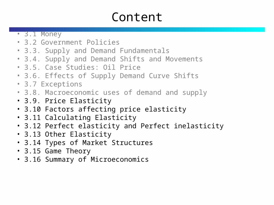
Content• 3.1 Money• 3.2 Government Policies• 3.3. Supply and Demand Fundamentals• 3.4. Supply and Demand Shifts and Movements• 3.5. Case Studies: Oil Price• 3.6. Effects of Supply Demand Curve Shifts• 3.7 Exceptions• 3.8. Macroeconomic uses of demand and supply• 3.9. Price Elasticity• 3.10 Factors affecting price elasticity• 3.11 Calculating Elasticity• 3.12 Perfect elasticity and Perfect inelasticity• 3.13 Other Elasticity• 3.14 Types of Market Structures• 3.15 Game Theory• 3.16 Summary of Microeconomics

3.9 Price Elasticity of demand

• It is useful to know how the quantity demanded or supplied will change when the price changes. This is known as the price elasticity of demand and the price elasticity of supply.

• If a monopolist decides to increase the price of their product, how will this affect their sales revenue?

Will the increased unit price offset the likely decrease in sales volume?

If a government imposes a tax on a good, thereby

increasing the effective price, how will this affect the

quantity demanded?

$


• Price elasticity of demand – An elasticity that measures the nature and degree of the

relationship between changes in quantity demanded of a good and changes in its price.


• For all normal goods, a price drop results in an increase in the quantity demanded by consumers.

• The demand for a good is relatively inelastic when the quantity demanded does not change much with the price change.

• Goods and services for which no substitutes exist are generally inelastic.


• Example– Demand for an antibiotic is highly inelastic when it alone

can kill an infection resistant to all other antibiotics.

– Rather than die of an infection, patients will generally be willing to pay whatever is necessary to acquire enough of the antibiotic to kill the infection.


• Necessities and Inelasticity– Inelastic demand is commonly associated with

"necessities," although there are many more reasons a good or service may have inelastic demand other than the fact that consumers may "need" it.


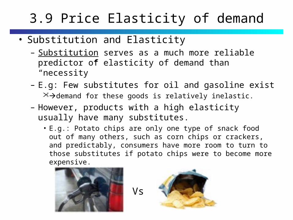
• Substitution and Elasticity – Substitution serves as a much more reliable predictor of

elasticity of demand than “necessity”

– E.g: Few substitutes for oil and gasoline exist demand for these goods is relatively inelastic.

– However, products with a high elasticity usually have many substitutes.

• E.g.: Potato chips are only one type of snack food out of many others, such as corn chips or crackers, and predictably, consumers have more room to turn to those substitutes if potato chips were to become more expensive.

Vs

3.10 Factors affecting price elasticity

• Factors affecting price elasticity– Availability of Substitutes

– The good is habit forming or obligatory

– The proportion of the consumer's income

– Duration of the demand shortage


• 3.10.1 Availability of Substitutes– Easily substitutable goods will enable buyers to switch to an alternative

good and thus such goods will exhibit greater elasticity than goods that do not have substitutes available

– It is important to understand that a given good is in essence unique and thus the comparability of the available substitutes in terms of quality to the original good is an important sub-variable.

– The better the substitutes can replace the original good in terms of desirability, affordability, practicality etc. the more elastic the good will become.


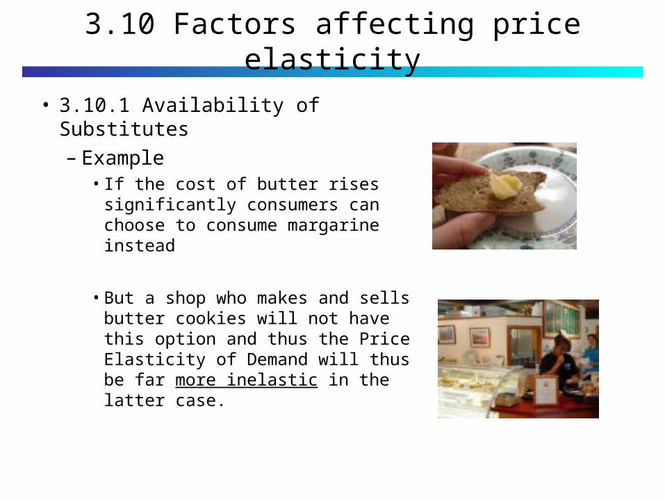
• 3.10.1 Availability of Substitutes– Example

• A driver used to use the Western Harbour Tunnel could switch to use the Central Harbour Tunnel if the Western Harbour Tunnel fares rise.

• However, it may be inconvenient and longer journey time and thus will form part of his consideration before switching the route

• It may take a certain price difference before he chooses this option representing the substitute's quality.


• 3.10.1 Availability of Substitutes– Example

• If the cost of butter rises significantly consumers can choose to consume margarine instead

• But a shop who makes and sells butter cookies will not have this option and thus the Price Elasticity of Demand will thus be far more inelastic in the latter case.


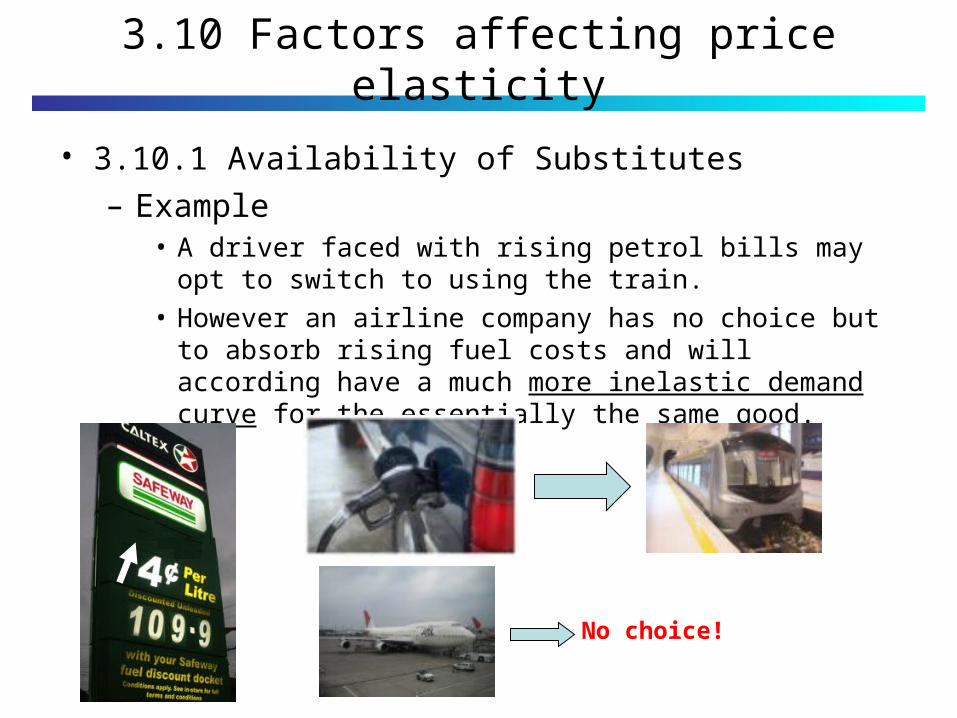
• 3.10.1 Availability of Substitutes – Example

• A driver faced with rising petrol bills may opt to switch to using the train.

• However an airline company has no choice but to absorb rising fuel costs and will according have a much more inelastic demand curve for the essentially the same good.

No choice!


• 3.10.2. The good is habit forming or obligatory– Addictive drugs, whether psychologically addictive or

physically addictive, and other goods where dependency plays a key role will naturally exhibit inelastic properties.

– At aggregate level, rising costs of such goods are unlikely to reduce demand significantly.

– Classic examples of such goods would be alcohol and tobacco.


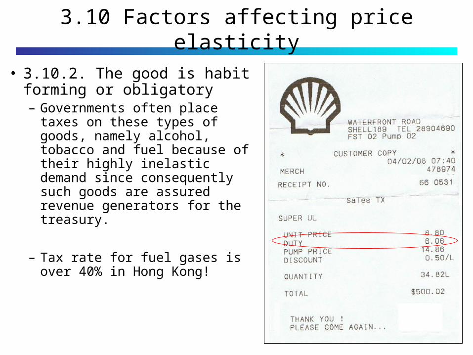
• 3.10.2. The good is habit forming or obligatory– Governments often place taxes

on these types of goods, namely alcohol, tobacco and fuel because of their highly inelastic demand since consequently such goods are assured revenue generators for the treasury.

– Tax rate for fuel gases is over 40% in Hong Kong!


• 3.10.3. The proportion of the consumer's income– Goods which typically make up a small proportion of

people's income will exhibit inelastic qualities.

– Conversely, goods which form a large proportion of people's income will cause greater responses in demand to comparable % increases or decreases in price.

– Example• If cinema ticket costs rise by 20%, decreases in demand are

unlikely to be pronounced.

• However a 15% drop in a "luxury" good such as a car or LCD Television changes in demand are likely to be relatively greater.


• 3.10.4. Duration of the demand shortage– Generally the greater the shortage period, the more

possible it may be for a good to be replaced with a substitute.

– Example: Home • A gas user faced with rising gas bills will unlikely be able

to switch to electric alternatives overnight due to possibly contractual tie-ins and time needed to change a stove to electric hob for example.

• However over 3 months, a switch is far more viable and the Price Elasticity of Demand will be accordingly more elastic.

– Likewise, prices are dynamic.• Over short time periods, prices of substitutes maybe static• Over longer periods, the price of substitutes may drop,

making them more appealing.

?

3.11 Calculating Elasticity

• Definitions

– Linear Elasticity • is the % change in one variable divided by the % change in another

variable

– Arc elasticity• calculates the elasticity over a range of values

– Point elasticity• uses differential calculus to determine the elasticity at a specific

point)

3.11. Calculation of Elasticity

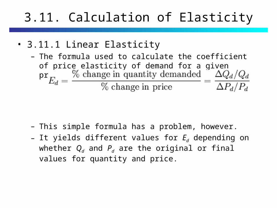
• 3.11.1 Linear Elasticity– The formula used to calculate the coefficient of price elasticity of

demand for a given product is

– This simple formula has a problem, however.

– It yields different values for Ed depending on whether Qd and Pd are the original or final values for quantity and price.


• 3.11.1 Linear Elasticity

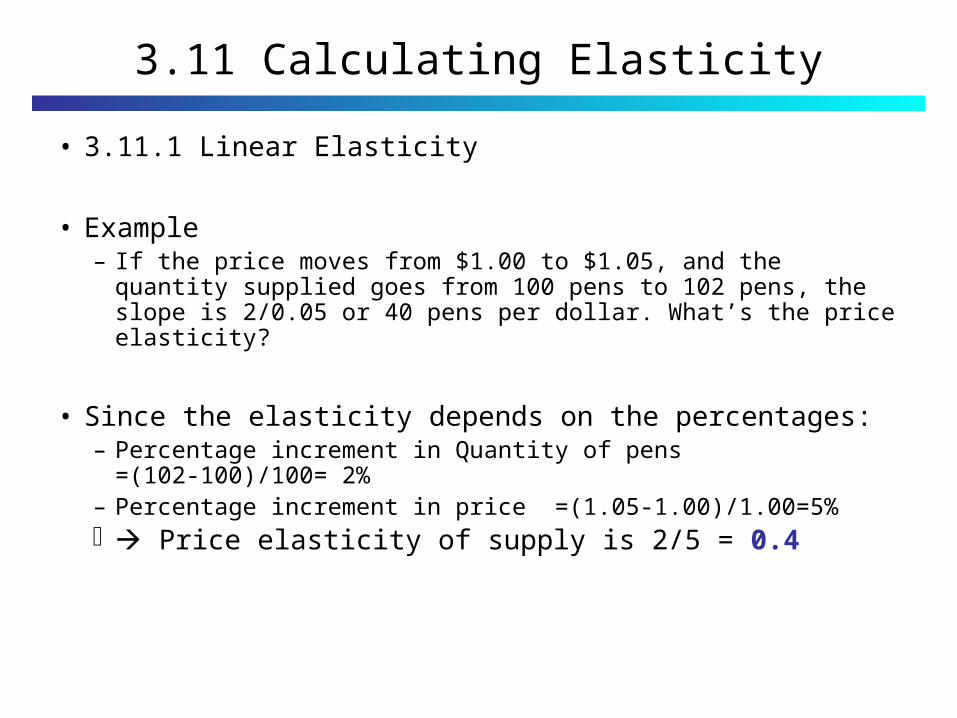
• Example– If the price moves from $1.00 to $1.05, and the quantity supplied

goes from 100 pens to 102 pens, the slope is 2/0.05 or 40 pens per dollar. What’s the price elasticity?

• Since the elasticity depends on the percentages:– Percentage increment in Quantity of pens =(102-100)/100= 2%– Percentage increment in price =(1.05-1.00)/1.00=5% Price elasticity of supply is 2/5 = 0.4


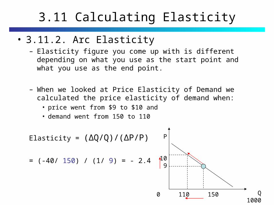
• 3.11.2. Arc Elasticity– Elasticity figure you come up with is different depending on what you

use as the start point and what you use as the end point.

– When we looked at Price Elasticity of Demand we calculated the price elasticity of demand when:

• price went from $9 to $10 and

• demand went from 150 to 110

Elasticity = (∆Q/Q)/(∆P/P)

= (-40/ 150) / (1/ 9) = - 2.4

Q1000

P

109

0 110 150


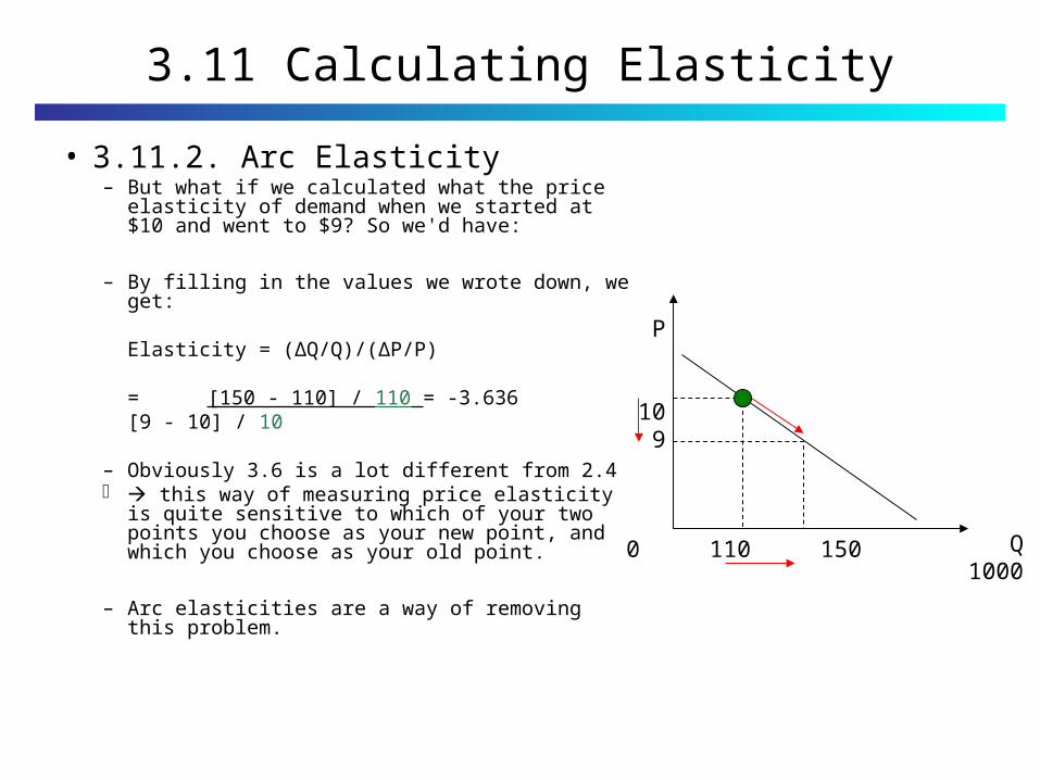
• 3.11.2. Arc Elasticity– But what if we calculated what the price elasticity of

demand when we started at $10 and went to $9? So we'd have:

– By filling in the values we wrote down, we get:

Elasticity = (∆Q/Q)/(∆P/P)

= [150 - 110] / 110 = -3.636[9 - 10] / 10

– Obviously 3.6 is a lot different from 2.4 this way of measuring price elasticity is quite

sensitive to which of your two points you choose as your new point, and which you choose as your old point.

– Arc elasticities are a way of removing this problem.

Q1000

P

109

0 110 150


• 3.11.2. Arc Elasticity

– When calculating Arc Elasticities, the basic relationships stay the same. So when we're calculating Price Elasticity of Demand we still use the basic formula:

Elasticity = % Change in Quantity Demanded

% Change in Price

Before

DemandNEW - DemandOLD

DemandOLD

DemandNEW – DemandOLD

½ ( DemandOLD + DemandNEW )

After: To calculate an arc-elasticity, we use the following formula:

This formula takes an average of the old quantity demanded and the new quantity demanded on the denominator.


• 3.11.2. Arc Elasticity

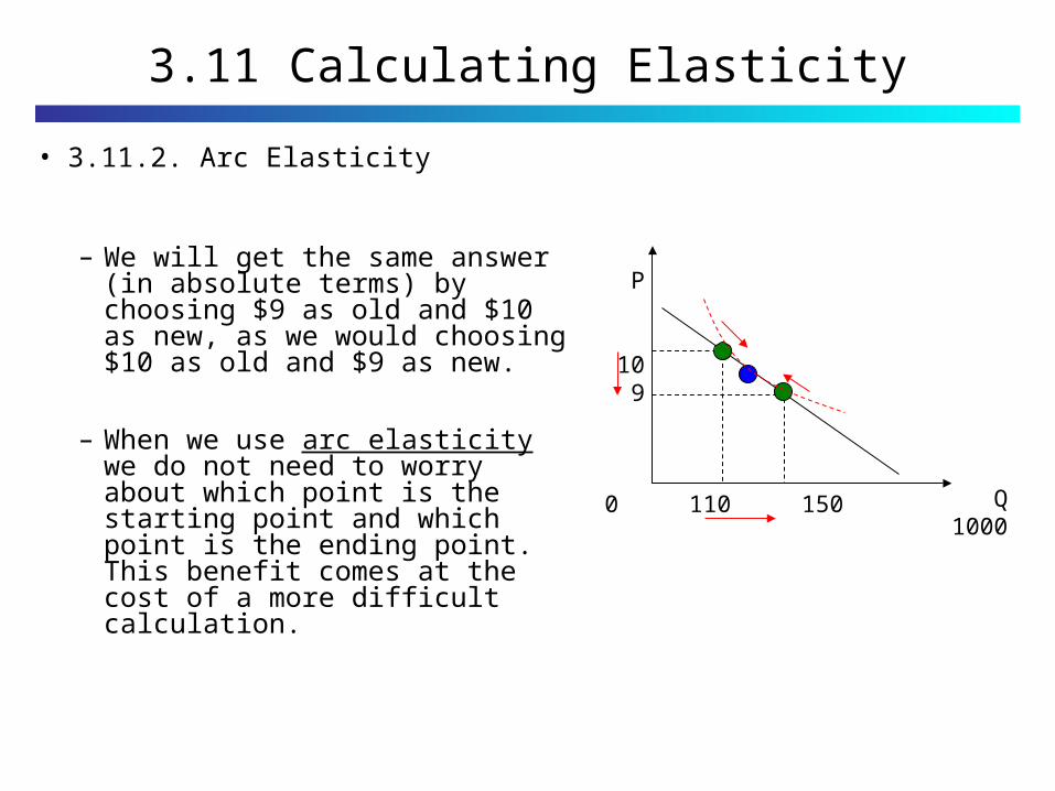
– We will get the same answer (in absolute terms) by choosing $9 as old and $10 as new, as we would choosing $10 as old and $9 as new.

– When we use arc elasticity we do not need to worry about which point is the starting point and which point is the ending point. This benefit comes at the cost of a more difficult calculation.

Q1000

P

109

0 110 150


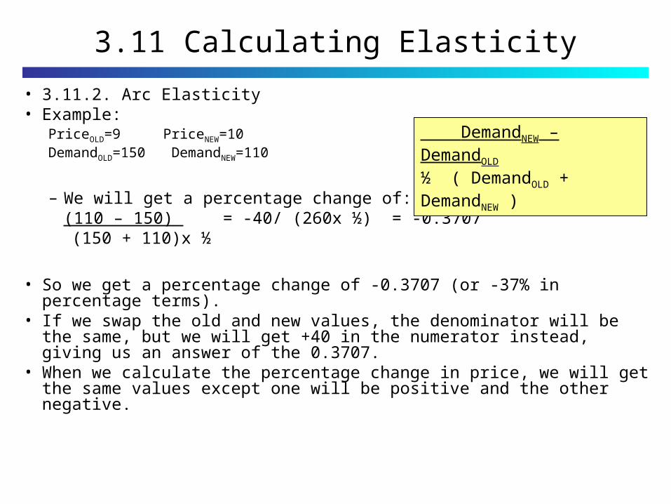
• 3.11.2. Arc Elasticity• Example:

PriceOLD=9 PriceNEW=10 DemandOLD=150 DemandNEW=110

– We will get a percentage change of:(110 – 150) = -40/ (260x ½) = -0.3707

(150 + 110)x ½

• So we get a percentage change of -0.3707 (or -37% in percentage terms).• If we swap the old and new values, the denominator will be the same, but

we will get +40 in the numerator instead, giving us an answer of the 0.3707. • When we calculate the percentage change in price, we will get the same

values except one will be positive and the other negative.

DemandNEW – DemandOLD

½ ( DemandOLD + DemandNEW )


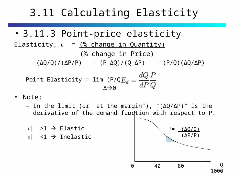
• 3.11.3 Point-price elasticityElasticity, = (% change in Quantity)

(% change in Price) = (∆Q/Q)/(∆P/P) = (P ∆Q)/(Q ∆P) = (P/Q)(∆Q/∆P)

Point Elasticity = lim (P/Q)(∆Q/∆P) =

∆0

• Note:– In the limit (or "at the margin"), "(∆Q/∆P)" is the derivative of the demand

function with respect to P.

>1 Elastic

<1 Inelastic

Q1000

P

0 40 80

= (∆Q/Q)(∆P/P)


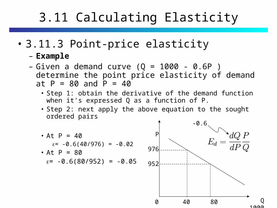
• 3.11.3 Point-price elasticity– Example– Given a demand curve (Q = 1000 - 0.6P ) determine the

point price elasticity of demand at P = 80 and P = 40• Step 1: obtain the derivative of the demand function when it's

expressed Q as a function of P.• Step 2: next apply the above equation to the sought ordered pairs

• At P = 40= -0.6(40/976) = -0.02

• At P = 80= -0.6(80/952) = -0.05

Q1000

P

976

952

0 40 80

-0.6


• 3.11.4. Total Revenue Test– It is a means for determining

whether demand is elastic or inelastic.

• If price Total revenue, (Pt A B)

– then demand can be said to be inelastic, since the increase in price does not have a large impact on quantity demanded.

• If price total revenue, (Pt.B C)

– then demand can be said to be elastic, since the increase in price has a large impact on quantity demanded.

Q1000

P

A

B

C

Area under the demand curve is the revenue


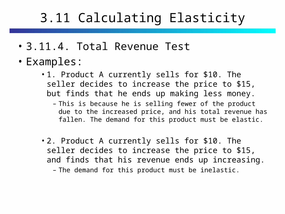
• 3.11.4. Total Revenue Test

• Examples:• 1. Product A currently sells for $10. The seller decides to

increase the price to $15, but finds that he ends up making less money.

– This is because he is selling fewer of the product due to the increased price, and his total revenue has fallen. The demand for this product must be elastic.

• 2. Product A currently sells for $10. The seller decides to increase the price to $15, and finds that his revenue ends up increasing.

– The demand for this product must be inelastic.

3.11 Elasticity and revenue

• 3.11.4. Total Revenue Test

– A set of graphs shows the relationship between demand and total revenue.

– In the elastic range (|| > 1), • Elasticity Revenue • Price Revenue

– In the inelastic range (|| < 1), • Elasticity Revenue • Price Revenue

Area under the

demand curve is

the revenue

elastic range Inelastic range

elastic range, decreasing

3.12 Perfect elasticity and Perfect inelasticity

• 3.11.4. Total Revenue Test– When the price elasticity of demand for a good is inelastic (|| < 1),

• the % change in quantity is smaller than that in price. when the price is raised, the total revenue of producers rises, and vice

versa.

– When the price elasticity of demand for a good is elastic (|| > 1),• the % change in quantity demanded is greater than that in price.• Hence, when the price is raised, the total revenue of producers falls, and

vice versa.

– When the price elasticity of demand for a good is unit elastic (or unitary elastic) (|| = 1),

• the % change in quantity is equal to that in price.


• Example - Find out the optimal pricing that maximize revenue:– Given a demand curve. – Determine the optimal price that maximize

revenueRevenue, R = Price x Qty

R = P x (1000-50P) = 1000P-50P2

Maximum when dR/ dP = 0

dR/dP = 1000 - 2x50P

dR/dP =0 P = 10 Q

P

20

10

0 500 1000

Q = 1000 - 50P

Q = 1000 - 50P

Mid Point is the Optimal Point!


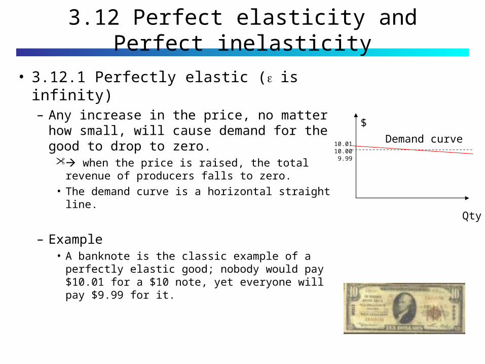
• 3.12.1 Perfectly elastic ( is infinity)– Any increase in the price, no matter how

small, will cause demand for the good to drop to zero. when the price is raised, the total revenue of

producers falls to zero.

• The demand curve is a horizontal straight line.

– Example• A banknote is the classic example of a perfectly

elastic good; nobody would pay $10.01 for a $10 note, yet everyone will pay $9.99 for it.

Qty

$

Demand curve10.0110.00 9.99


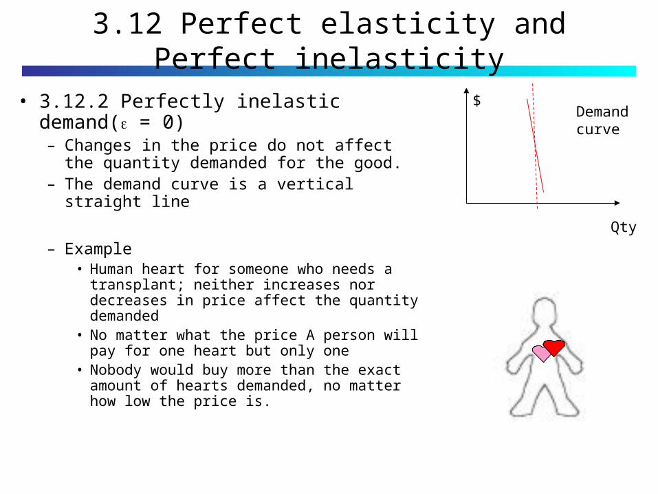
• 3.12.2 Perfectly inelastic demand( = 0) – Changes in the price do not affect the quantity

demanded for the good. – The demand curve is a vertical straight line

– Example• Human heart for someone who needs a

transplant; neither increases nor decreases in price affect the quantity demanded

• No matter what the price A person will pay for one heart but only one

• Nobody would buy more than the exact amount of hearts demanded, no matter how low the price is.

Qty

$Demand curve


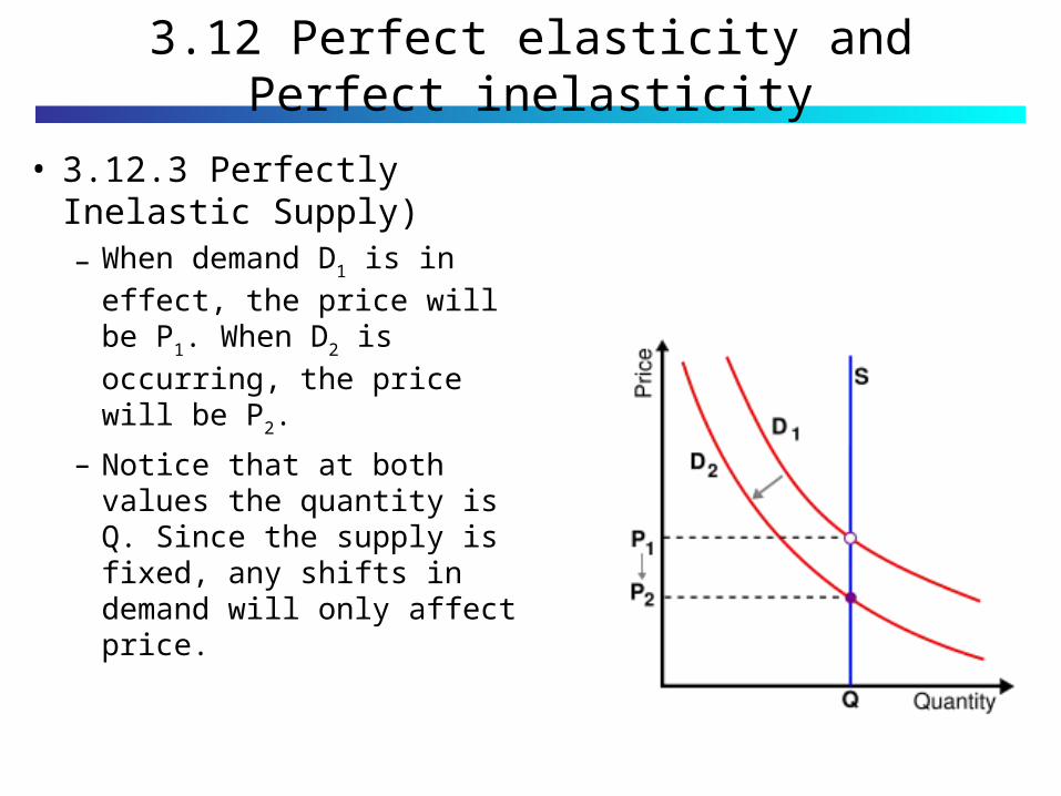
• 3.12.3. Perfectly Inelastic Supply (Vertical supply curve )– An example of perfectly inelastic supply, or zero

elasticity, is represented as a vertical supply curve– When demand D1 is in effect, the price will be P1.

– When D2 is occurring, the price will be P2.

– Notice that at both values the quantity is Q. Since the supply is fixed, any shifts in demand will only affect price.


• 3.12.3 Perfectly Inelastic Supply)– When demand D1 is in effect,

the price will be P1. When D2

is occurring, the price will be P2.

– Notice that at both values the quantity is Q. Since the supply is fixed, any shifts in demand will only affect price.


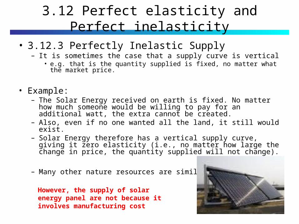
• 3.12.3 Perfectly Inelastic Supply– It is sometimes the case that a supply curve is vertical

• e.g. that is the quantity supplied is fixed, no matter what the market price.

• Example:– The Solar Energy received on earth is fixed. No matter how much

someone would be willing to pay for an additional watt, the extra cannot be created.

– Also, even if no one wanted all the land, it still would exist. – Solar Energy therefore has a vertical supply curve, giving it zero

elasticity (i.e., no matter how large the change in price, the quantity supplied will not change).

– Many other nature resources are similar

However, the supply of solar energy panel are not because it involves manufacturing cost

3.13. Other Elasticity

• Other Elasticity in relation to other variables– Price elasticity of supply– Income elasticity of demand– Cross elasticity of demand

3.13 Other Elasticity

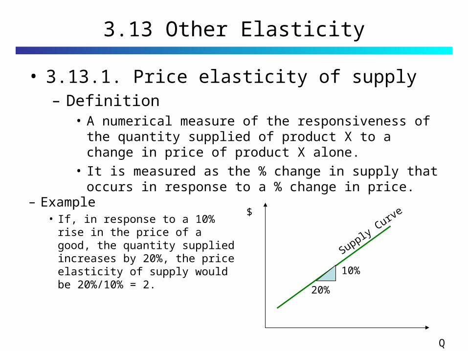
• 3.13.1. Price elasticity of supply– Definition

• A numerical measure of the responsiveness of the quantity supplied of product X to a change in price of product X alone.

• It is measured as the % change in supply that occurs in response to a % change in price.

– Example• If, in response to a 10% rise in

the price of a good, the quantity supplied increases by 20%, the price elasticity of supply would be 20%/10% = 2.

Q

$

10%

20%

Supply Curve


• 3.13.1. Price elasticity of supply– In the short term:

• The supply quantity can be different from the amount produced, as manufacturers will have stocks which they can build up or run down.

– In the long run:• However, quantity supplied and quantity produced are

synonymous.


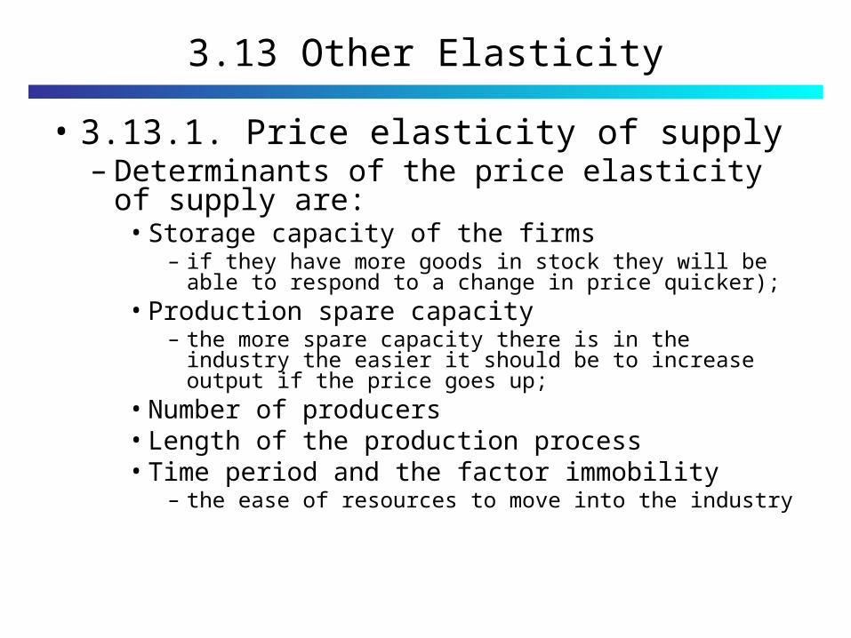
• 3.13.1. Price elasticity of supply – Determinants of the price elasticity of supply are:

• Storage capacity of the firms – if they have more goods in stock they will be able to respond

to a change in price quicker); • Production spare capacity

– the more spare capacity there is in the industry the easier it should be to increase output if the price goes up;

• Number of producers• Length of the production process• Time period and the factor immobility

– the ease of resources to move into the industry


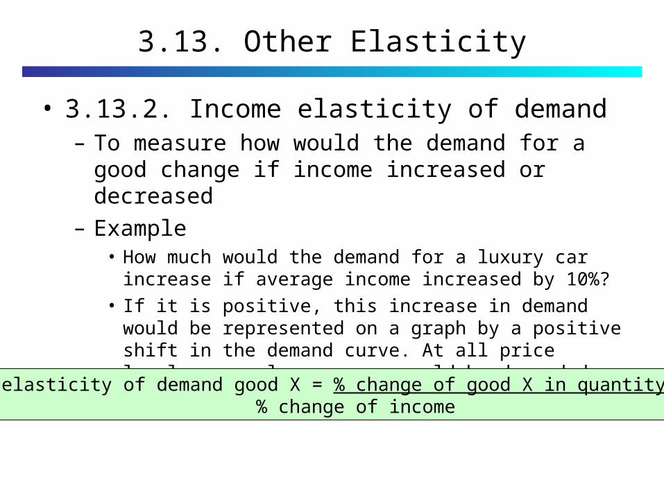
• 3.13.2. Income elasticity of demand– To measure how would the demand for a good change if

income increased or decreased

– Example• How much would the demand for a luxury car increase if average

income increased by 10%?

• If it is positive, this increase in demand would be represented on a graph by a positive shift in the demand curve. At all price levels, more luxury cars would be demanded.

Income elasticity of demand good X = % change of good X in quantity demand% change of income


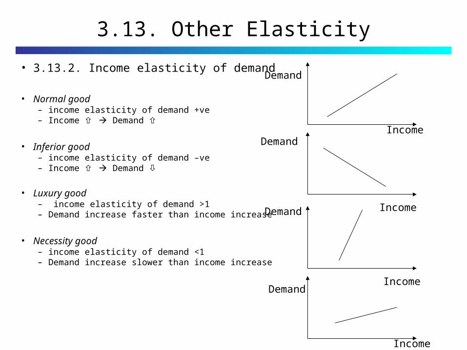
• 3.13.2. Income elasticity of demand

• Normal good – income elasticity of demand +ve– Income Demand

• Inferior good– income elasticity of demand –ve– Income Demand

• Luxury good– income elasticity of demand >1 – Demand increase faster than income increase

• Necessity good– income elasticity of demand <1 – Demand increase slower than income increase

Income

Income

Income

Income

Demand

Demand

Demand

Demand


• 3.13.3 Cross elasticity of demand– It measures the responsiveness of the quantity demanded of a good to a

change in the price of another good. – This is often considered when looking at the relative changes in

demand when studying complement and substitute goods.

– Complement goods are goods that are typically utilized together, where if one is consumed, usually the other is also.

• E.g. Bread and Butter, Coffee and Milk, Fuel and Car; Computers and Software

– Substitute goods are those where one can be substituted for the other, and if the price of one good rises, one may purchase less of it and instead purchase its substitute.


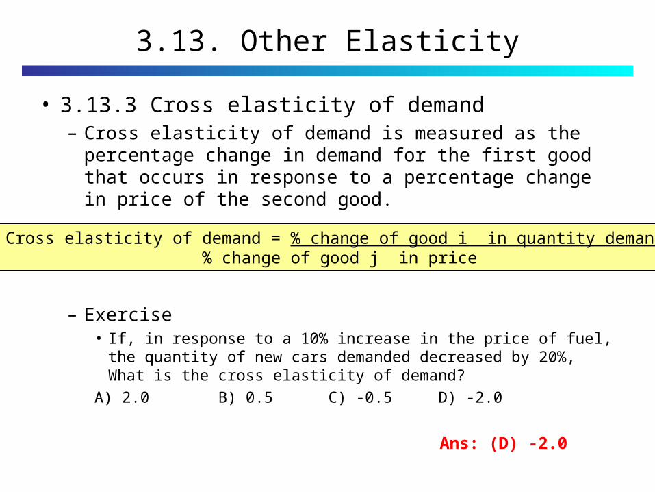
• 3.13.3 Cross elasticity of demand– Cross elasticity of demand is measured as the percentage

change in demand for the first good that occurs in response to a percentage change in price of the second good.

– Exercise• If, in response to a 10% increase in the price of fuel, the quantity of

new cars demanded decreased by 20%, What is the cross elasticity of demand?

A) 2.0 B) 0.5 C) -0.5 D) -2.0

Cross elasticity of demand = % change of good i in quantity demand % change of good j in price

Ans: (D) -2.0

3.14 Types of Market Structures

• Basic Market Structures– There are four types of Market

Structures• Perfect Competition

– Considerable no of Similar Firms

• Monopoly – One Firm

• Oligopoly – Few Firms

• Monopolistic Competition – Many Firms show product differentiation


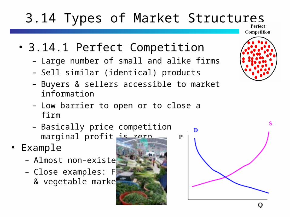
• 3.14.1 Perfect Competition– Large number of small and alike firms

– Sell similar (identical) products

– Buyers & sellers accessible to market information

– Low barrier to open or to close a firm

– Basically price competition until marginal profit is zero.

• Example– Almost non-existent.

– Close examples: Fruit & vegetable market.


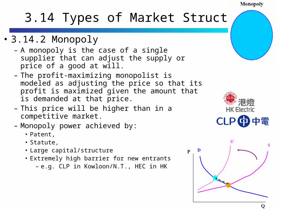
• 3.14.2 Monopoly– A monopoly is the case of a single supplier that can

adjust the supply or price of a good at will. – The profit-maximizing monopolist is modeled as

adjusting the price so that its profit is maximized given the amount that is demanded at that price.

– This price will be higher than in a competitive market.

– Monopoly power achieved by:• Patent,• Statute, • Large capital/structure • Extremely high barrier for new entrants

– e.g. CLP in Kowloon/N.T., HEC in HK


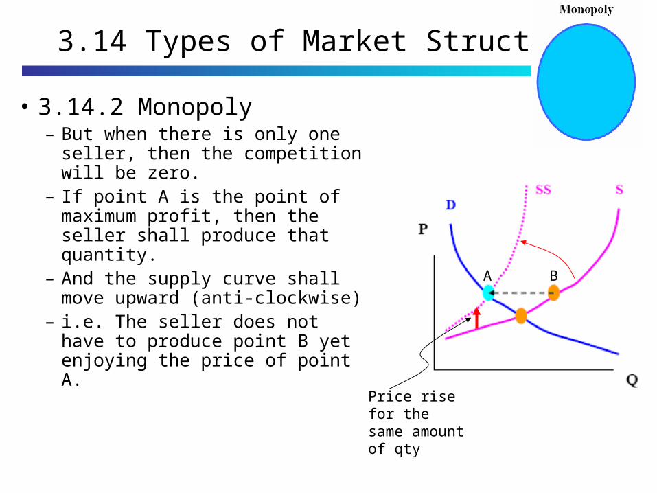
• 3.14.2 Monopoly– But when there is only one seller,

then the competition will be zero.– If point A is the point of

maximum profit, then the seller shall produce that quantity.

– And the supply curve shall move upward (anti-clockwise)

– i.e. The seller does not have to produce point B yet enjoying the price of point A.

A B

Price rise for the same amount of qty


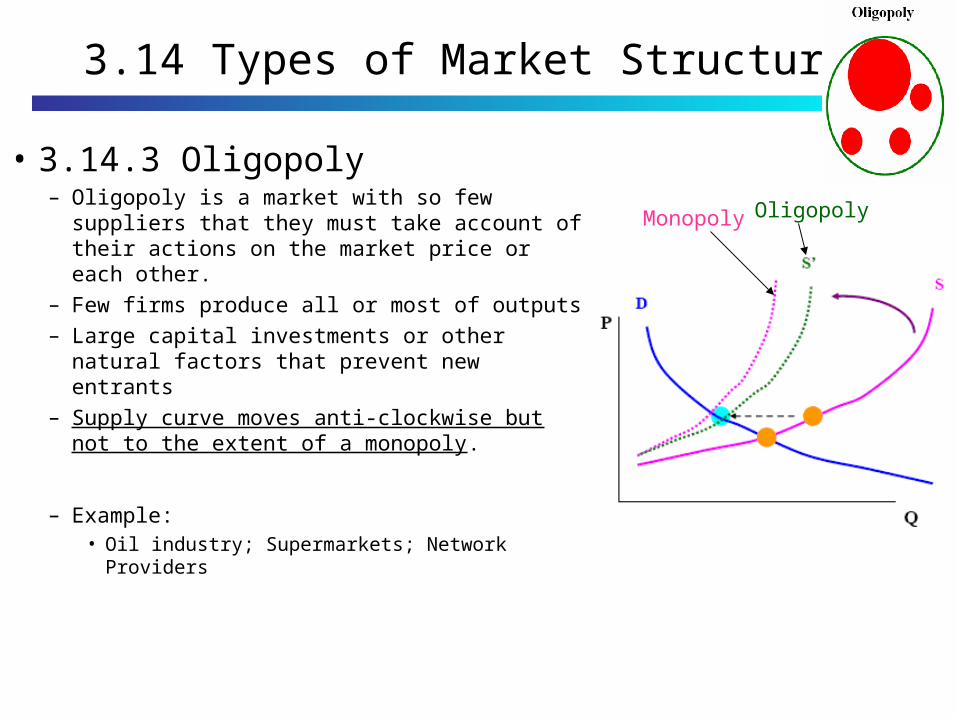
• 3.14.3 Oligopoly– Oligopoly is a market with so few suppliers

that they must take account of their actions on the market price or each other.

– Few firms produce all or most of outputs

– Large capital investments or other natural factors that prevent new entrants

– Supply curve moves anti-clockwise but not to the extent of a monopoly.

– Example:• Oil industry; Supermarkets; Network Providers

Monopoly Oligopoly


• 3.14.3 Oligopoly– If there are many firms in the market, but a few dominates

the market, with an extremely high concentration ratio of market shares, is also treated as an Oligopoly.

– In general, Oligopoly can be healthy if the firms maintain sufficiently keen and clean competition.

– It is common for oligopoly firms to produce explicit or implicit collaboration called Cartel ( 企業聯合 ) (alliance)

– When Cartel arrangements become “illegal”, they’re called Collusion ( 勾結 ).


• 3.14.4 Monopolistic Competition– Many firms in the market

• Firms produce similar products but differentiates from each other (product differentiation to create “monopoly” power)

• Entry barrier is medium

• As products are different, it’s hard to define a single demand curve and a single supply curve for the whole category

• Perhaps we may view each differentiated product individually, or look it them as a superposition of all the curves.

– e.g. Stationery, drinks, many convenience goods.


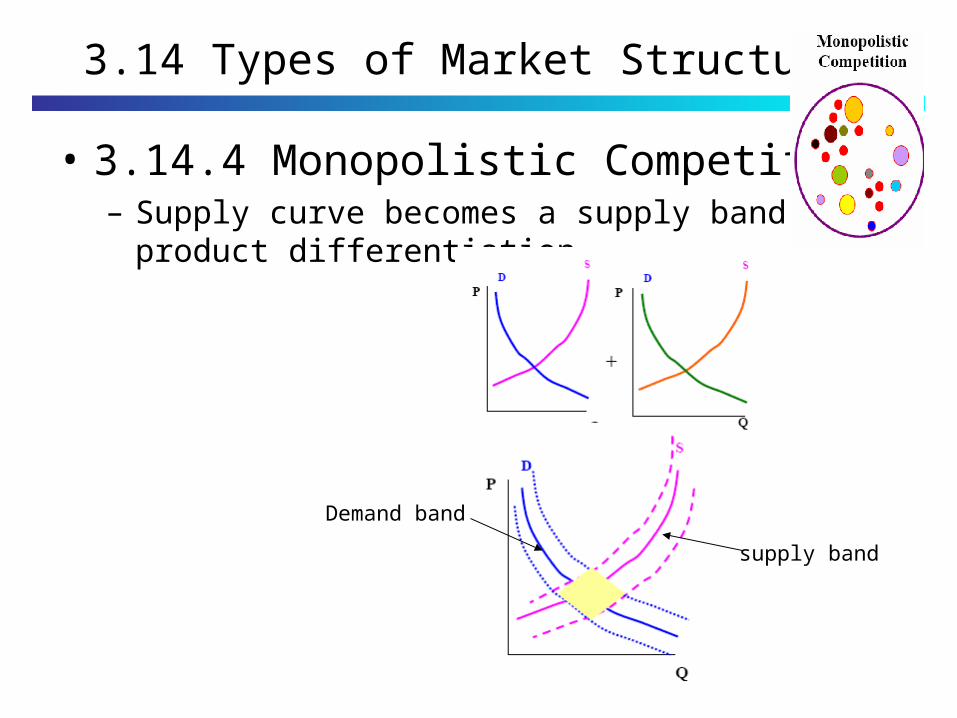
• 3.14.4 Monopolistic Competition– Supply curve becomes a supply band by product

differentiation.

supply band

Demand band

3.15 Game theory

• The above example, with two sellers only, is an oligopoly.

• The outcome in which Peter and Mary each produce 40 gallons looks like some sort of equilibrium. This outcome is called Nash Equilibrium, named after economic theorist John Nash.

• A Nash Equilibrium is a situation in which economic actors interacting with one another each choosing their best strategy given the strategies the others have chosen.

• That leads to the use of Game Theory. One well known and typical example is the Prisoners’ Dilemma.

3.15 Game Theory

• 3.15.1 The prisoners’ dilemma– A story about two criminals who have been captured by the

police. Let’s call them Peter & David.– The Police have enough evidence to convict Peter & David

of the minor crime of posting erotic photos on the internet, so that each would spend 1 year in jail.

– The police also suspect that the two criminals have committed blackmail together, but they lack the hard evidence to convict them of this major crime, unless one of them admits.

– The police question Peter & David in separate rooms, and they offer each of them the following deal:

3.15 Game Theory

“Right now, we can lock you up for 1 year. If you admit blackmail and implicate your partner, however we’ll give you immunity and you can go free. Your partner will get 20 years in jail.

But if you both admit to the crime, we won’t need your testimony and we can avoid the cost of a trial, so you will each get an immediate sentence of 8 years.”

3.15 Game Theory

• If you are Peter who cares only about his own sentences, what would you do?

• However, you don’t know for sure what choice that David will make. – Reference: N G Mankiw, Principles of Economics 2nd ed.,

Harcourt

– A) Stay Silent

– B) Admit blackmail and implicate David

3.15 Game Theory

• The dilemma arises when one assumes that both prisoners only care about minimizing their own jail terms.

• Each prisoner has 2 options: – to co-operate with his partner and stay quiet, or

– to betray his partner in return for a lighter sentence.

• The outcome of each choice depends on the choice of their partner, but each prisoner must choose without knowing what his partner has chosen.

• In deciding what to do in strategic situations, it is normally important to predict what others will do.

A

BA

3.15 Game Theory

• If you knew the other prisoner would stay silent, – your best move is to betray as you then walk free instead of receiving the minor

sentence.

• If you knew the other prisoner would betray, – your best move is still to betray, as you receive a lesser sentence than by silence.

• The other prisoner reasons similarly, and therefore also chooses to betray.

• One may think that he would get a shorter jail period (8 yrs vs 20 yrs) if he betrays than if he stays silent.

But in fact it is worse off than if they both had stayed silent (1 yr vs 8 yrs)

Peter Stays Silent Peter Betrays

David Stays Silent Each serves 1 years David serves 20 yearsPeter goes free

David Betrays David goes freePeter serves 20 years

Each serves 8 years

3.15 Game Theory

• The prisoner's dilemma is a type of non-zero-sum game in which two players may be "cooperative” or “uncooperative” with each other.

• In most of the game theory game, the only concern of each individual player ("prisoner") is maximizing his/her own payoff, without any concern for the other player's payoff.

• In this case, a rational choice leads the two players to both play uncooperatively even though each player's individual reward would be greater if they both are cooperative.

3.15 Game Theory

• Who innovate the Game Theory?– John Nash visited

HKU in 2003 and presented the Game Theory

3.15 Game Theory

• How was the Game Theory innovated?

• A Beautiful Mind is a 2001 biographical film about John Forbes Nash, the Nobel Laureate (Economics) mathematician.

• The story begins in the early years of Nash's life at Princeton University as he develops his "original idea" that will revolutionize the world of mathematics.

• It won four Academy Awards, including– Best Picture,– Best Director, – Best Adapted Screenplay, and – Best Supporting Actress.

• The film has been criticized for its inaccurate portrayal of some aspects of Nash's life.

Let’s watch a movie

3.15 Game Theory: A Beautiful MindSource: http://www.youtube.com/watch?v=2d_dtTZQyUM&feature=related

3.15 Game Theory

• What we have learnt from the movie?– “Best result comes from everyone in the group doing what's best

for himself. Incomplete. Incomplete. Because the best result will come when everyone in the group doing what's best for himself and the group.”

John Nash– John Nash proved mathematically that complete self-interest is

not in the best interest of the group.– “Adam Smith's theory is incomplete. Self-interest alone can lead

to disaster for all” John Nash demonstrated mathematically. – Self-interest coupled with concern for the good of the group is

most likely to benefit everyone.

3.15 Game Theory

• More about John Nash and the Game Theory

• http://obelix.lib.hku.hk/av/feature.html

References

• http://en.wikipedia.org/wiki/Price_elasticity_of_demand

• http://obelix.lib.hku.hk/av/feature.html• http://obelix.lib.hku.hk/av/feature.html• http://www.netmba.com/econ/micro/demand/elasticit

y/price/• http://economics.about.com/cs/micfrohelp/a/priceelas

ticity.htm

Documents

ELEC15- Engineering Economics & Finance Day 4 Session 3: Microeconomics-2 Dr. Wilton W.T. Fok Room CYC703 Tel: 2857 8490