Embed Size (px)
Citation preview

12/4/2017
1
1
Solving RLC Circuits: Instructions
When you are presented with a switched or pulsed RLC circuit
and asked to solve for v(t) or i(t) somewhere in the circuit, for all time…
(1) Identify the circuit as containing two (and only two) energy storage elements
(i.e. a single Leq and a single Ceq).
(2) Determine 1 initial condition just before the switch/pulse, e.g. v(0–) .
(3) Determine 2 conditions just after the switch/pulse, e.g. v(0+) and d/dtv(0+) ,
with the knowledge that vC(0–) = vC(0+) , iL(0–) = iL(0+) ,
iC(0+) = C d/dtvC(0+), vL(0+) = L d/dtiL(0+) .
(4) Determine final conditions (a long time after the switch/pulse), e.g. v(∞) .
(5) Identify the circuit as a series or parallel RLC circuit
and find the Thevenin equivalent resistance seen by the LC pair, Rth .
(6) Calculate α and ω0 and determine the circuit damping (over, under, critical) .
(7) Assume the appropriate solution form and use α, ω0, initial conditions,
& the final condition to determine the complete (particular) solution.
All slides and content courtesy of Dr. Gregory J. Mazzaro
ELEC 201 – Electric Circuit Analysis I
Lecture 9(d)
RLC Circuit
Example
3
Solve for vR(t) for all values of t
and determine the settling time ts .
Example: RLC Circuit #1
4
Solve for vR(t) for all values of t
and determine the settling time ts .
( )0 48 VRv−
=
( )0 48 VRv+
=
( ) 0 VR
v ∞ =
( )0 0R
dv
dt
+=
overdamped
• Find 4 boundary conditions
& decide on the damping…
• Assume the appropriate form for t > 0 and solve for all 5 unknowns…
( ) 1 2
1 2 3
s t s tx t X e X e X= + + 2 2
1,2 0s α α ω= − ± −
Example: RLC Circuit #1
( ) ( ) ( )
( ) ( )0
15
2 24 1 240
124
10 1 240
α
ω
= =
= =
12/4/2017
2
5
Solve for vR(t) for all values of t
and determine the settling time ts .
( )0 48 VRv −=
( )0 48 VRv +=
( ) 0 VRv ∞ =
( )0 0R
dv
dt
+=
( ) 1 2
1 2 3
c t c t
Rv t V e V e V= + +05.0 , 4.9α ω= =
2 2
1,2 1 25.0 5.0 4.9 4, 6c c c= − ± − ⇒ ≈ − ≈ −2 2
1,2 0c α α ω= − ± −
( ) 4 6
1 2 3
t t
Rv t V e V e V
− −= + +
Substituting 2 of the 5 unknowns
into the overdamped solution…
Example: RLC Circuit #1
6
Solve for vR(t) for all values of t
and determine the settling time ts .
( )0 48 VRv −=
( )0 48 VRv +=
( ) 0 VRv ∞ =
( )0 0R
dv
dt
+=
( ) 4 6
1 2 3
t t
Rv t V e V e V
− −= + +
Making use of the initial & final conditions…
( ) 1 2 30 48 VR
v V V V+
= + + =
( ) 3 0 VR
v V∞ = =( ) 1 20 4 6 0R
dv V V
dt
+= − − =
Solving the 3 equations with 3 unknowns…1 2 3144 V , 96 V, 0V V V= = − =
Example: RLC Circuit #1
7
Solve for vR(t) for all values of t
and determine the settling time ts .
( ) 4 6
48 V 0
144 96 V 0R t t
tv t
e e t− −
<=
− >
Example: RLC Circuit #1
8
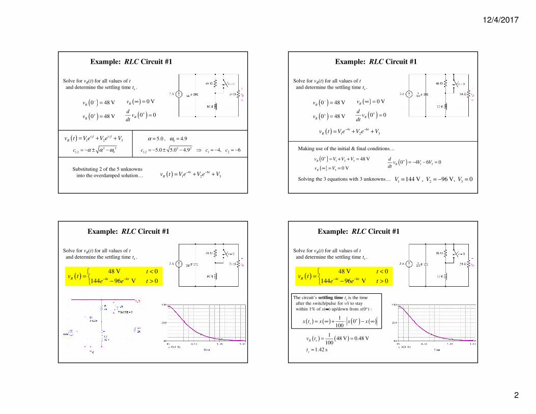
Solve for vR(t) for all values of t
and determine the settling time ts .
The circuit’s settling time ts is the time
after the switch/pulse for v/i to stay
within 1% of x(∞∞∞∞) up/down from x(0+) :
( ) ( ) ( ) ( )1
0100
sx t x x x+
≈ ∞ + ⋅ − ∞
( ) ( )1
48 V 0.48 V100
1.42 s
R s
s
v t
t
= =
≈
( ) 4 6
48 V 0
144 96 V 0R t t
tv t
e e t− −
<=
− >
Example: RLC Circuit #1

12/4/2017
3
9
Solve for vR(t) for all values of t
and determine the settling time ts .
t = 0:1e-3:1.5;
v_R = 144*exp(-4*t) - 96*exp(-6*t);
plot(t,v_R)
axis([0 1.5 0 50])
grid
ylabel('v_R (volts)')
xlabel('Time (seconds)')
( ) 4 6
48 V 0
144 96 V 0R t t
tv t
e e t− −
<=
− >
Example: RLC Circuit #1
All content courtesy of Dr. Gregory J. Mazzaro
ELEC 201 – Electric Circuit Analysis I
Lecture 9(e)
More RLC Circuit
Examples
11
Is the circuit (at right) underdamped,
overdamped, or critically damped?
Example: RLC Circuit #2
12
Is the circuit (at right) underdamped,
overdamped, or critically damped?
th0
1,
2
R
L LCα ω= =series RLC:
R is the Thevenin equivalent resistance
seen by the L & C in series…
A
B
no independent sources
must use a test source to find RthItest
Vtest
+
–
Example: RLC Circuit #2

12/4/2017
4
13
Is the circuit (at right) underdamped,
overdamped, or critically damped?
th0
1,
2
R
L LCα ω= =series RLC:
ItestVtest
+
–
test 1 A, 1 AI i= =
( ) ( ) ( ) ( )test
test
9 1 3 1 2 1 0
8 V
V
V
− + − + =
=
choose the test current:
solve for the test voltage:
their ratio is Rth: th test test8R V I= = Ω
Example: RLC Circuit #2
14
Is the circuit (at right) underdamped,
overdamped, or critically damped?
th0
1,
2
R
L LCα ω= =series RLC:
( ) ( )th 8 rad
0.82 2 5 s
R
Lα = = =
α < ω0, underdamped
( ) ( )0
3
1 1 rad10
s5 2 10LCω
−= = =
⋅
Example: RLC Circuit #2
15
PSpice: RLC Circuit #2
Is the circuit (at right) underdamped,
overdamped, or critically damped?
oscillates, therefore
underdamped
16
( )2 Vsv u t=
Is the circuit (below) underdamped,
overdamped, or critically damped?
235 Ω
4.7
nF
1
mHsv
Analog Discovery: RLC Circuit #3

12/4/2017
5
17
( )2 Vsv u t=
Analog Discovery: RLC Circuit #3
18
Analog Discovery: RLC Circuit #3
19
no oscillation, therefore
overdamped
Analog Discovery: RLC Circuit #3
20
1.5 kΩ
4.7
nF
1
mHsv
Is the circuit (below) underdamped,
overdamped, or critically damped?
( )2 Vsv u t=
Analog Discovery: RLC Circuit #4

12/4/2017
6
21
Analog Discovery: RLC Circuit #4
22
Analog Discovery: RLC Circuit #4
oscillates, therefore
underdamped
23
Example: RLC Circuit #5
Determine the damping of this circuit
(after t = 0).
24
After the switch closes, the circuit becomes
0
1 1,
2RC LCα ω= =For a parallel RLC circuit,
( ) ( )5
9
1 rad1.3 10
s2 200 20 10α
−= = ⋅
⋅ ( )( )5
03 9
1 rad10
s5 10 20 10ω
− −= =
⋅ ⋅
α > ω0, overdamped
Example: RLC Circuit #5
Determine the damping of this circuit
(after t = 0).

12/4/2017
7
25
PSpice: RLC Circuit #5
Determine the damping of this circuit
(after t = 0).
no oscillation, therefore
overdamped
26
PSpice: RLC Circuit #5
Determine the damping of this circuit
(after t = 0).
no oscillation, therefore
overdamped
27
Solve for i1(t) for all values of t
and plot i1 from t = 0 to t = ts .
Example: RLC Circuit #6
28
Solve for i1(t) for all values of t
and plot i1 from t = 0 to t = ts .
• Find 4 boundary conditions
& decide on the damping…
( ) ( )1
10 3 A 1.5 A
2i
−= − = −
( )0 0Li−
=
( ) ( ) ( )
( ) ( )
1 1
1
0 2 0 0 0
0 3 0 4.5 V
C
C
v i i
v i
− − −
− −
− − =
= = −
Before the step…
Example: RLC Circuit #6

12/4/2017
8
29
Solve for i1(t) for all values of t
and plot i1 from t = 0 to t = ts .
• Find 4 boundary conditions
& decide on the damping…
Just after the step…
( ) ( )0 0 0L L
i i− += =
( ) ( ) ( ) ( ) ( )1 10 0 2 0 0 0
C Lv i i v+ + + +
− + − − − =
KVL around right loop…
KVL around outer loop…
( ) ( ) ( ) ( ) ( )1 10 0 2 0 0 0C L
v i i v+ + + +
− − − − − =
( )1 0 0i+
=
( ) ( )0 0
4.5 V
L Cv v+ +
= −
=
vL
+
–
i1
Example: RLC Circuit #6
30
Solve for i1(t) for all values of t
and plot i1 from t = 0 to t = ts .
• Find 4 boundary conditions
& decide on the damping…
Also note:
( ) ( )1
10 0
2L
i i+ += − ( ) ( )
( )
( )
1
10 0
2
1 10
2
1 1 A4.5 0.225
2 10 s
L
L
d di i
dt dt
vL
+ +
+
= −
= −
= − = −
Just after the step…
Example: RLC Circuit #6
31
Solve for i1(t) for all values of t
and plot i1 from t = 0 to t = ts .
• Find 4 boundary conditions
& decide on the damping…
A long time after the step…
( ) 0Li ∞ =
( ) 0Cv ∞ =
( )1 0i ∞ =
(no independent source)
Example: RLC Circuit #6
32
Solve for i1(t) for all values of t
and plot i1 from t = 0 to t = ts .
• Find 4 boundary conditions
& decide on the damping…
We need Rth seen by the L, C to decide on the damping…
A
BVtest
+
–
Itest
choose Itest = 2 A…
test1 1 A
2
Ii = =
( ) ( ) ( )test
test
1 1 2 1 0
3 V
V
V
− + − − =
=
th test test1.5R V I= = Ω
Example: RLC Circuit #6

12/4/2017
9
33
Solve for i1(t) for all values of t
and plot i1 from t = 0 to t = ts .
• Find 4 boundary conditions
& decide on the damping…
For a series RLC circuit,
th0
1,
2
R
L LCα ω= =
( ) ( )
1.5 rad0.075
2 10 sα = =
( ) ( )0
1 rad0.316
s10 1ω = =
0α ω<
underdamped
( ) ( ) ( )1 1 2 3cos sint
d di t e I t I t I
α ω ω−= + +
…therefore the solution is of the form
Example: RLC Circuit #6
34
• Solve for I1, I2, I3…
Solve for i1(t) for all values of t
and plot i1 from t = 0 to t = ts .
( ) ( ) ( )1 1 2 3cos sint
d di t e I t I t I
α ω ω−= + +
( )10i ∞ =( )1
A0 0.225
s
di
dt
+= −
( )1 0 1.5 Ai−
= − ( )1 0 0 Ai+
=
( ) ( ) ( )0
1 1 2 3 1 30 cos 0 sin 0 0
d di e I I I I Iω ω+ −
= ⋅ + ⋅ + = + =
( ) ( )2 22 2
0 .316 .075
0.307 rad s
dω ω α= − = −
=
( ) ( ) ( )1 1 2 3 30 cos sin 0
d di I t I t I Iω ω∞ = ⋅ ⋅ + ⋅ + = =
( ) ( ) ( ) ( ) ( )1 1 2 1 2
1 2
0 cos sin sin cos
0.075 0.307 0.225
t t
d d d d d d
di e I t I t e I t I t
dt
I I
α αα ω ω ω ω ω ω+ − −= − + + − +
= − ⋅ + ⋅ = −
1
2
3
0 A
733 mA
0 A
I
I
I
=
= −
=
Example: RLC Circuit #6
35
Solve for i1(t) for all values of t
and plot i1 from t = 0 to t = ts .
( ) ( ) ( ) ( )
( ) ( )
1 1 1 1
1
10
100
1733 mA
100
s
s
i t i i i
i t
+≈ ∞ + − ∞
≈( )
0.0751
100
ln 1 100 0.075
4.6 0.075
st
s
s
e
t
t
−≈
≈ − ⋅
− ≈ − ⋅
60 ss
t ≈
( )( )1 0.075
1500 mA 0
733 sin 0.307 mA 0t
ti t
e t t−
− <=
− ⋅ ⋅ >
Example: RLC Circuit #6
36
Solve for i1(t) for all values of t
and plot i1 from t = 0 to t = ts .
t = -10:.1:100;
alpha = 0.075;
omega_d = 0.307;
I_1 = 0; I_2 = -733e-3; I_3 = 0;
i = (t>0).*(exp(-alpha*t).*(I_1*cos(omega_d*t) ...
+ I_2*sin(omega_d*t)) + I_3) + ...
(t<0).* -1.5;
plot(t,i,'Linewidth',2)
axis([-10 50 -1.6 0.4])
grid
ylabel('i_1 (A)')
xlabel('Time (s)')
( )( )1 0.075
1500 mA 0
733 sin 0.307 mA 0t
ti t
e t t−
− <=
− ⋅ ⋅ >
Matlab: RLC Circuit #6

12/4/2017
10
37
Solve for i1(t) for all values of t
and plot i1 from t = 0 to t = ts .
( )( )1 0.075
1500 mA 0
733 sin 0.307 mA 0t
ti t
e t t−
− <=
− ⋅ ⋅ >
PSpice: RLC Circuit #6