Einführung in Mathematica

Grundlegendes

Ausführen von Befehlen

4 + 1

5

H3 + 6L *7^2�70063

����������100

H* Symbolisches Rechnen *L2 a + 5 a

8490, 469, 532<Ha + bL Ha - bL8-50325, -234632, -6545<Expand@Ha + bL Ha - bLD8-50325, -234632, -6545<Simplify@a^2 - 2 a b + b^2D827225, 178084, 1225<H* Ergebniss unterdrücken *L4 + 1;

H* Befehle hintereinander ausführen *L2^104^55^23

1024

1024

11920928955078125

H* Sequenz *Lx = 1 ; y = x + 1; y + x

3

Eine Sequenz ist ein einfacher Ausdruck, und kann Funktionen als Parameter übergeben werden.Wichtig für das imperative Programmieren mit Mathematica.

Exp@x = 1; y = x + 1; y + xDã3

Syntax

Kommentare: (* ... *)Ausdrücke gruppieren: ( )Funktionsparamter: [ ]Listen, Mengen, Matrizen: { }Indizierung: [[ ]]

Zugriff auf berechnete Ergebnisse

2 + 3;

H* Aufrufen des zuletzt berechneten Ergebnisses *LSqrt@%D�!!!!5H* Aufrufen des vorletzten Ergebnisses *LSqrt@%%D�!!!!5H* Numerische Berechnung *LN@%D2.23607

Variablen und Zuweisungen

a = 2 + 3

5

2 mathematica_einfuehrung.nb

c = Sqrt@aD�!!!!5a = 10

10

c

�!!!!5H* Löschen von Variablen *LClear@a, cDa

a

b = 5

5

H* Alternativ mit dem Unset-Operator =. *Lb =.

b

b

Elementare Funktionen und Konstanten

Pi

Π

mathematica_einfuehrung.nb 3

N@Pi, 1000D3.14159265358979323846264338327950288419716939937510582097494459230781�640628620899862803482534211706798214808651328230664709384460955058223�172535940812848111745028410270193852110555964462294895493038196442881�097566593344612847564823378678316527120190914564856692346034861045432�664821339360726024914127372458700660631558817488152092096282925409171�536436789259036001133053054882046652138414695194151160943305727036575�959195309218611738193261179310511854807446237996274956735188575272489�122793818301194912983367336244065664308602139494639522473719070217986�094370277053921717629317675238467481846766940513200056812714526356082�778577134275778960917363717872146844090122495343014654958537105079227�968925892354201995611212902196086403441815981362977477130996051870721�134999999837297804995105973173281609631859502445945534690830264252230�825334468503526193118817101000313783875288658753320838142061717766914�730359825349042875546873115956286388235378759375195778185778053217122�6806613001927876611195909216420199

H* Eulersche Zahl *LE

ã

N@ED2.71828

H* Komplexe Einheit *LI

ä

I^2

-1

Cos@PiD-1

Sin@PiD0

Tan@PiD0

4 mathematica_einfuehrung.nb

Cot@PiDComplexInfinity

Exp@PiD - E^Pi

0

Log@E^2D2

Log@10, 100D2

Hilfe

?Sin

Sin@zD gives the sine of z. Mehr¼

?? Solve

Solve@eqns, varsD attempts to solve an equation or set of equations forthe variables vars. Solve@eqns, vars, elimsD attempts to solvethe equations for vars, eliminating the variables elims. Mehr¼

Attributes@SolveD = 8Protected<Options@SolveD = 8InverseFunctions ® Automatic,MakeRules ® False, Method ® 3, Mode ® Generic, Sort ® True,VerifySolutions ® Automatic, WorkingPrecision ® ¥<

Ausdrücke und Funktionen

Ausdrücke

Clear@xDf = 1 + Sqrt@xD1 +

�!!!!xf

1 +�!!!!x

mathematica_einfuehrung.nb 5

H* f ist keine Funktion *Lf@1DI1 +

�!!!!x M@1DH* Substitution *Lf �. x ® 1

2

Funktionen

Clear@f, xDBeim definieren von Funktionen müsssen die Variablen als Pattern (z.B.: var_ ) deklariert werden.

f@x_D := 1 + Sqrt@xD;f@3D1 +

�!!!!3Clear@gDACHTUNG!Die folgende Gleichung definiert keine Funktion.

g@xD := 1 + Sqrt@xDg@3Dg@3DMittelwert@x_, y_D := Hx + yL �2;Mittelwert@3, 5D4

"Set" und "SetDelayed"

Clear@ff, xD

6 mathematica_einfuehrung.nb

x = 4;

Bei Funktionsdefinitionen mittels "Set (=)" wird die rechte Seite sofort evaluiert.

ff@x_D = 2 x;

ff@xDff@3Dff@yD8

8

8

Clear@ff, xDx = 4;

Bei Funktionsdefinitionen mittels "SetDelayed (:=)" wird die rechte Seite lazy evaluiert.Dies ist normalerweise das gewünsche Verhalten.

ff@x_D := 2 x;

ff@xDff@3Dff@yD8

6

4

z = 3;

Globable Variablen sind trotzdem möglich.

gg@x_D := 2 x + z

mathematica_einfuehrung.nb 7

gg@xDgg@3Dgg@yD11

9

7

Listen, Mengen und Matrizen

Listen

li = 8a, b, c, d<8a, b, c, d<H* Zugriff auf Elemente *LFirst@liDLast@liDli@@1DDli@@3DDli@@-1DDli@@81, 3<DDa

d

a

c

d

8a, c<Append@li, aD8a, b, c, d, a<

8 mathematica_einfuehrung.nb

Length@liDReverse@liDDelete@li, 2D4

8d, c, b, a<8a, c, d<H* Aneinanderhängen von Listen *LJoin@li, 81, 2, 3<D8a, b, c, d, 1, 2, 3<

Erzeugen und Manipulieren von Listen

Range@10D81, 2, 3, 4, 5, 6, 7, 8, 9, 10<Range@5, 10D85, 6, 7, 8, 9, 10<Range@1, 10, 3D81, 4, 7, 10<Table@i^2, 8i, 1, 10<D81, 4, 9, 16, 25, 36, 49, 64, 81, 100<range = Range@10D;MemberQ@range, 5DMemberQ@range, 11DTrue

False

f@x_D := x^2;Map@f, 81, 2, 3, 4, 5<D81, 4, 9, 16, 25<

mathematica_einfuehrung.nb 9

H* Anonyme Funktionen *LMap@#^2 &, 81, 2, 3, 4, 5<D81, 4, 9, 16, 25<H* Elemente auswählen *LSelect@range, # > 5 && # < 8 &D86, 7<Nest@# + 1 &, 1, 5D6

Clear@fDNest@f, a, 5Df@f@f@f@f@aDDDDDSum@i, 8i, 1, 100<DProduct@i, 8i, 1, 100<D5050

9332621544394415268169923885626670049071596826438162146859296389521759�999322991560894146397615651828625369792082722375825118521091686400000�0000000000000000000

Mengen

li2 = 8a, c, e, f<8a, c, e, f<Union@li, li2D8a, b, c, d, e, f<Intersection@li, li2D8a, c<

10 mathematica_einfuehrung.nb

Complement@li, li2DComplement@li2, liD8b, d<8e, f<Subsets@Range@5DD88<, 81<, 82<, 83<, 84<, 85<, 81, 2<, 81, 3<, 81, 4<, 81, 5<, 82, 3<, 82, 4<,82, 5<, 83, 4<, 83, 5<, 84, 5<, 81, 2, 3<, 81, 2, 4<, 81, 2, 5<, 81, 3, 4<,81, 3, 5<, 81, 4, 5<, 82, 3, 4<, 82, 3, 5<, 82, 4, 5<, 83, 4, 5<, 81, 2, 3, 4<,81, 2, 3, 5<, 81, 2, 4, 5<, 81, 3, 4, 5<, 82, 3, 4, 5<, 81, 2, 3, 4, 5<<

Matrizen

A = 881, 2, 3<, 86, 3, 4<, 83, 4, 5<<881, 2, 3<, 86, 3, 4<, 83, 4, 5<<A �� MatrixForm

ikjjjjjj1 2 36 3 43 4 5

y{zzzzzzA �� TableForm

1 2 36 3 43 4 5

Det@AD8

Inverse@AD �� MatrixForm

ikjjjjjjjjjjjj

- 1����8

1����4

- 1����8

- 9����4

- 1����2

7����4

15������8

1����4

- 9����8

y{zzzzzzzzzzzz

mathematica_einfuehrung.nb 11

H* Matrix Multiplikation *LA . Inverse@AD �� MatrixForm

ikjjjjjj1 0 00 1 00 0 1

y{zzzzzzH* Multiplication mit Skalar *L2 A �� MatrixForm

ikjjjjjj2 4 612 6 86 8 10

y{zzzzzzA@@1, 1DD = 0; A �� MatrixForm

ikjjjjjj0 2 36 3 43 4 5

y{zzzzzzPolynome

Clear@f, x, yDf = Hx + yL^10 - Hx + y^2L^5Hx + yL10 - Hx + y2L5Expand@fD-x5 + x10 + 10 x9 y - 5 x4 y2 + 45 x8 y2 + 120 x7 y3 - 10 x3 y4 + 210 x6 y4 +252 x5 y5 - 10 x2 y6 + 210 x4 y6 + 120 x3 y7 - 5 x y8 + 45 x2 y8 + 10 x y9

Collect@f, xDx10 + 10 x9 y + 45 x8 y2 + 120 x7 y3 + 210 x6 y4 + x5 H-1 + 252 y5L +x4 H-5 y2 + 210 y6L + x3 H-10 y4 + 120 y7L + x2 H-10 y6 + 45 y8L + x H-5 y8 + 10 y9LCollect@f, yD-x5 + x10 + 10 x9 y + H-5 x4 + 45 x8L y2 + 120 x7 y3 + H-10 x3 + 210 x6L y4 +252 x5 y5 + H-10 x2 + 210 x4L y6 + 120 x3 y7 + H-5 x + 45 x2L y8 + 10 x y9

12 mathematica_einfuehrung.nb

Factor@fDx H-1 + x + 2 yLHx4 + x5 + x6 + x7 + x8 + 2 x4 y + 4 x5 y + 6 x6 y + 8 x7 y + 5 x3 y2 + 9 x4 y2 +

17 x5 y2 + 29 x6 y2 + 10 x3 y3 + 28 x4 y3 + 62 x5 y3 + 10 x2 y4 + 30 x3 y4 +86 x4 y4 + 20 x2 y5 + 80 x3 y5 + 10 x y6 + 50 x2 y6 + 20 x y7 + 5 y8L

Collect@f, x, FactorDx10 + 10 x9 y + 45 x8 y2 + 120 x7 y3 + 210 x6 y4 + 5 x y8 H-1 + 2 yL +5 x2 y6 H-2 + 9 y2L + 10 x3 y4 H-1 + 12 y3L + 5 x4 y2 H-1 + 42 y4L + x5 H-1 + 252 y5LCoefficient@f, x, 5D-1 + 252 y5

Coefficient@f, x^5D-1 + 252 y5

Exponent@f, xDExponent@f, x, MinD10

1

Exponent@f, yDExponent@f, y, MinD9

0

Analysis

Differentation

f = HSin@xD + Cos@xD^2L �Exp@xDã-x HCos@xD2 + Sin@xDLD@f, xD-ã-x HCos@xD2 + Sin@xDL + ã-x HCos@xD - 2 Cos@xD Sin@xDL

mathematica_einfuehrung.nb 13

H* 3. Ableitung nach x *LD@f, 8x, 3<D-ã-x HCos@xD2 + Sin@xDL + 3 ã-x HCos@xD - 2 Cos@xD Sin@xDL +

ã-x H-Cos@xD + 8 Cos@xD Sin@xDL - 3 ã-x H-2 Cos@xD2 - Sin@xD + 2 Sin@xD2LIntegration

H* Unbestimmtes Integral *LIntegrate@f, xD-

1�������10

ã-x H5 + 5 Cos@xD + Cos@2 xD + 5 Sin@xD - 2 Sin@2 xDLD@%, xD-

1�������10

ã-x H5 Cos@xD - 4 Cos@2 xD - 5 Sin@xD - 2 Sin@2 xDL +

1�������10

ã-x H5 + 5 Cos@xD + Cos@2 xD + 5 Sin@xD - 2 Sin@2 xDLTrigFactor@%D1�����2

ã-x H1 + Cos@2 xD + 2 Sin@xDLTrigFactor@fD1�����2

ã-x H1 + Cos@2 xD + 2 Sin@xDLH* Bestimmtes Integral *LIntegrate@f, 8x, 0, Pi<D1

�������10

H11 - ã-ΠLGrenzwerte

Limit@f, x ® InfinityD0

H* Grenzwert von links *LLimit@Tan@xD, x ® Π �2, Direction ® 1D¥

14 mathematica_einfuehrung.nb

H* Grenzwert von rechts *LLimit@Tan@xD, x ® Π �2, Direction ® -1D-¥

Symbolische Summen, Reihen

Sum@Binomial@n, iD 2^i, 8i, 0, n<D3n

Sum@1�i^2, 8i, 1, Infinity<DΠ2�������6

Symbolische Summen, Reihen

Sum@Binomial@n, iD 2^i, 8i, 0, n<D3n

Sum@1�i^2, 8i, 1, Infinity<DΠ2�������6

Grafik

Plot@Sin@xD + 1�2 Sin@2 xD + 1�4 Sin@2 xD, 8x, -Pi, Pi<D;

-3 -2 -1 1 2 3

-1.5

-1

-0.5

0.5

1

1.5

sinus = Table@Sin@x�10D, 8x, 1, 10^2<D;

mathematica_einfuehrung.nb 15

ListPlot@sinusD;

20 40 60 80 100

-1

-0.5

0.5

1

data = Table@8Cos@2 Pi x�20D, Sin@2 Pi x�20D<, 8x, 0, 20<D;ListPlot@data, PlotStyle ® 8PointSize@0.02D, Hue@0.7D<D;

-1 -0.5 0.5 1

-1

-0.5

0.5

1

16 mathematica_einfuehrung.nb

ListPlot@data, PlotJoined ® True, AspectRatio ® 1D;

-1 -0.5 0.5 1

-1

-0.5

0.5

1

Zahlentheorie

Euklidscher Algorithmus

H* Grösster gemeinsamer Teiler *LGCD@10, 15D5

ExtendedGCD@10, 15D85, 8-1, 1<<-1*10 + 1*15

5

H* Kleinstes gemeinsame Vielfache *LLCM@3, 4D12

GCD@2^2000 - 1, 3^1000 - 1D7145813125

mathematica_einfuehrung.nb 17

LCM@2^2000 - 1, 3^1000 - 1D2124195053270864771981385349571935831438980704980214484288980526676186�540337515520522368836851166261013165008729933741953544430162468464479�727461751151186344340945575858445926557266109885553627022228068783067�040585006640638208533320190808275570827485467618046904626080806824528�840421461862226415218170859165014941661612049604504369676960036923727�771267696427801070371508919605420590848320560475919989351827463726020�350764672836561764653224810275232738962409653825074880963423855162968�865272204060219037456940242749175725036178704374797419964970110566982�926207887564682912430080876423119914999972920369919548816517800613073�234429690810649717169538014283725989657747813120374611674289590357451�713469666802110705158488226888475560168433950863086094880326909910491�359355342398790980602125753813674562269490545450522533471918821702710�837319468010696342036223002322664482136921408812124958808978590137757�522338385567379743015312833980532537456968809973101980377711288035224�970808722357196893324274068159757092314801932147690662785428141728386�7070862085086201236153484021340000

Primzahlen und Faktorisierung

H* Berechnen der n-ten Primzahl *LPrime@1D2

Prime@10^9D22801763489

H* Liste der ersten 100 Primzahlen *LTable@Prime@iD, 8i, 1, 100<D82, 3, 5, 7, 11, 13, 17, 19, 23, 29, 31, 37, 41, 43, 47, 53, 59, 61, 67,71, 73, 79, 83, 89, 97, 101, 103, 107, 109, 113, 127, 131, 137, 139,149, 151, 157, 163, 167, 173, 179, 181, 191, 193, 197, 199, 211, 223,227, 229, 233, 239, 241, 251, 257, 263, 269, 271, 277, 281, 283,293, 307, 311, 313, 317, 331, 337, 347, 349, 353, 359, 367, 373,379, 383, 389, 397, 401, 409, 419, 421, 431, 433, 439, 443, 449,457, 461, 463, 467, 479, 487, 491, 499, 503, 509, 521, 523, 541<

H* Primzahl Test *LPrimeQ@19DPrimeQ@20DTrue

False

H* 20. Mersienne Primzahl H1961L *LTiming@PrimeQ@2^4423 - 1DD84.42633 Second, True<

18 mathematica_einfuehrung.nb

<< NumberTheory‘PrimeQ‘

ProvablePrimeQ@19DProvablePrimeQ@20DTrue

False

p = NextPrime@2^200D1606938044258990275541962092341162602522202993782792835301611

Timing@ProvablePrimeQ@pDDTiming@PrimeQ@pDD84.85626 Second, True<80.005999 Second, True<H* Primfaktorisierung *Lfactors = FactorInteger@2^200 - 1D883, 1<, 85, 3<, 811, 1<, 817, 1<, 831, 1<, 841, 1<, 8101, 1<,8251, 1<, 8401, 1<, 8601, 1<, 81801, 1<, 84051, 1<, 88101, 1<,861681, 1<, 8268501, 1<, 8340801, 1<, 82787601, 1<, 83173389601, 1<<MultiplyFactors@list_D := Times �� Map@#@@1DD^#@@2DD &, listDMultiplyFactors@factorsD == 2^200 - 1

True

Restklassen

Mod@67, 20DQuotient@76, 20D7

3

Timing@Mod@3^10000000, 77DD83.25651 Second, 67<

mathematica_einfuehrung.nb 19

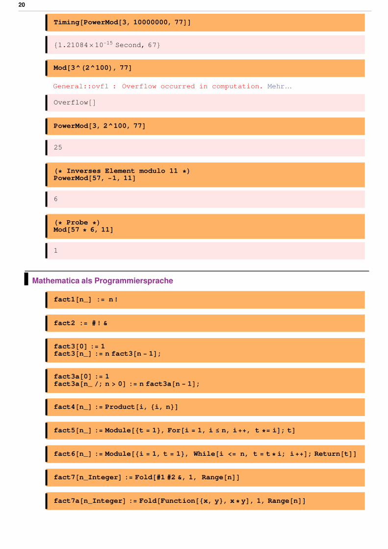
Timing@PowerMod@3, 10000000, 77DD81.21084´10-15 Second, 67<Mod@3^H2^100L, 77DGeneral::ovfl : Overflow occurred in computation. Mehr¼

Overflow@DPowerMod@3, 2^100, 77D25

H* Inverses Element modulo 11 *LPowerMod@57, -1, 11D6

H* Probe *LMod@57 * 6, 11D1

Mathematica als Programmiersprache

fact1@n_D := n!

fact2 := #! &

fact3@0D := 1fact3@n_D := n fact3@n - 1D;fact3a@0D := 1fact3a@n_ �; n > 0D := n fact3a@n - 1D;fact4@n_D := Product@i, 8i, n<Dfact5@n_D := Module@8t = 1<, For@i = 1, i £ n, i++, t *= iD; tDfact6@n_D := Module@8i = 1, t = 1<, While@i <= n, t = t*i; i++D; Return@tDDfact7@n_IntegerD := Fold@#1 #2 &, 1, Range@nDDfact7a@n_IntegerD := Fold@Function@8x, y<, x*yD, 1, Range@nDD

20 mathematica_einfuehrung.nb

fact7list@n_IntegerD := FoldList@#1 #2 &, 1, Range@nDDMyFold@f_, e_, 8<D := e;MyFold@f_, e_, list_D := MyFold@f, f@e, First@listDD, Rest@listDDfact8@n_IntegerD := MyFold@#1 #2 &, 1, Range@nDDfact9@n_D := Times �� Range@nDfact10@n_D := Apply@Times, Range@nDDfact11@n_ �; n ³ 0D := If@n � 0, 1, n fact11@n - 1DDfact12 = If@#1 == 0, 1, #1 #0@#1 - 1DD &;

à Laufzeitvergleiche

Timing@fact1@50000D;D80.286956 Second, Null<Timing@fact4@50000D;D80.453931 Second, Null<Timing@fact5@50000D;D85.8851 Second, Null<Timing@fact6@50000D;D85.8861 Second, Null<Timing@fact7@50000D;D85.18921 Second, Null<Timing@fact10@50000D;D80.411937 Second, Null<

mathematica_einfuehrung.nb 21