Embed Size (px)
Citation preview
Eindhoven University of Technology
MASTER
Stereo coding by two-channel linear prediction and rotation
Selten, T.P.J.
Award date:2004
DisclaimerThis document contains a student thesis (bachelor's or master's), as authored by a student at Eindhoven University of Technology. Studenttheses are made available in the TU/e repository upon obtaining the required degree. The grade received is not published on the documentas presented in the repository. The required complexity or quality of research of student theses may vary by program, and the requiredminimum study period may vary in duration.
General rightsCopyright and moral rights for the publications made accessible in the public portal are retained by the authors and/or other copyright ownersand it is a condition of accessing publications that users recognise and abide by the legal requirements associated with these rights.
• Users may download and print one copy of any publication from the public portal for the purpose of private study or research. • You may not further distribute the material or use it for any profit-making activity or commercial gain
Take down policyIf you believe that this document breaches copyright please contact us providing details, and we will remove access to the work immediatelyand investigate your claim.
Download date: 14. Jul. 2018
9~2..{
Eindhoven University of Technology Department of Electrical Engineering Signal Processing Systems TU/e
Stereo coding by two-channel linear
prediction and rotation
Master of Science thesis
Project period: 09-2003- 10-2004 Report Number: 19-04
Commissioned by:
Supervisors: Dr.ir. A.C. den Brinker (Philips Research) Ddr. L.L.M. Vogten (TU/e)
Additional Commission members: Prof.dr.ir. J.W.M. Bergmans (TU/e)
by T.P.J. Selten
The Department of Electrical Engineering of the Eindhoven University of Technology accepts no responsibility for the contents of M.Sc. theses or practical training reports
technische
universiteit eindhoven
TECHNISCHE UNIVERSITEIT EINDHOVEN
Department of Electrical Engineering
MASTER'S THESIS
Stereo coding by two-channel linear prediction and rotation
Supervisors
by
T.P.J. Selten
prof. dr. ir. J.W.M. Bergmans (TU/e) dr. ir. L.L.M. Vogten (TU /e) dr. ir. A.C. den Brinker (Philips Research)
Eindhoven, 20th October 2004

" If it will take ten years to make the machine with available technology, and only five years to make it with a new technology, and it will only take two years to invent the new technology, then you can do it in seven years by inventing the new technology first! "
NEAL STEPHENSON IN CRYPTONOMICON, 1999
Summary
In the context of an M.Sc. graduation project at Philips Research Laboratories in Eindhoven, this thesis concerns stereo coding as part of an audio coder. Audio coding aims at removing redundancies and irrelevancies from the audio signal to reduce the bit rate. Stereo coding aims at exploiting cross-channel redundancies and irrelevancies to attain a lower bit rate than the sum of the independently coded channels.
Desired is a stereo coding technique which allows perfect reconstruction at the high bit rate end (e.g., in the absence of quantization), and which is able to compete with the latest stereo coding methods at the low bit rates.
Known stereo coding methods, briefly discussed in this thesis, do not meet the desired criteria. The most efficient technique is parametric stereo coding (Binaural Cue Coding (BCC) and Optimal Coding of Stereo ( OSC)) which separates the signal into audio content and spatial information. By reducing the two audio channels to one and some side information, very low bit rates are achieved. However, the original can not be reconstructed perfectly.
In this thesis, we propose to use a two-channel (stereo) Linear Predictor (LP), based on FIR or IIR (Laguerre) filters in combination with a single rotator. A linear estimate of the current signal is made from the history of both channels. The LP allows perfect reconstruction. For the prediction filters Laguerre filters are chosen, because of their close resemblance to the psycho-acoustical Bark-scale, which is advantageous for lossy audio coding.
Optimizing the proposed system dissolves in two separate stages: optimizing the stereo LP and subsequently optimizing the rotator with the residual from the Stereo LP. An efficient way of optimizing the Stereo LP is using the block-Levinson algorithm, which only applies under the condition of equal orders of auto and cross predictors. Furthermore, two preliminary ideas for quantization of these optimal parameters are introduced in this thesis.
Stability of the proposed system is examined more closely in this thesis, the stability being determined through the synthesis filter of the Stereo LP. It is argued that stability is only guaranteed when equal orders of auto and cross predictors are used.
The proposed system is implemented in Matlab in combination with C, and works as expected. Preliminary experiments have been conducted to establish which parts of the residual signal have to be maintained in a transmission system and which parts can be compromised. Unlike the situation in BCC and OCS, the side signal can apparently not be discarded completely without causing problems, but fair results are already achieved by only transmitting 10% of the side signal, i.e. only low frequencies. Other methods are examined that would allow low bit rate coding and the most promising method appears to be Spectral Band Replication (SBR). This technique is very suitable due to the spectrally flat character of residual signals. With SBR only a part of the total bandwidth is transmitted, and this is applicable to both the main and the side signal. This suggests that low bit rate coders based on the proposed system are feasible.

Confidential
ll

Preface
The thesis before you is the result of my nine-months' graduation project, which has been conducted at Philips Research in order to obtain the degree Master of Science in Electrical Engineering from the University of Technology in Eindhoven (TU /e). This project has been initiated by the Audio Coding cluster, which is part of the Digital Signal Processing (DSP) group. This project was accepted under the responsibility of the research chair Signal Processing Systems, which is part of the capacity group Measurement and Control Systems at the department of Electrical Engineering of TU je.
Through this project I've seen, and participated in a larger research project aimed at developing audio coding algorithms. Thus I got involved in different stages of that project ranging from the stage of an early idea-like, the starting point of this project, until extensive listening tests for finished coders. It also let me "re-discover" music, which was gradually been pushed to the background. Attentive listening sometimes required for this project rubbed of to "normal" music listening, intensifying the experience, with maybe the exception of some excerpts of music and speech used for testing.
I would like to acknowledge the institutions and individuals that made it possible to deliver this thesis. First of all Philips Research Eindhoven which provided an inspiring working environment for this thesis, and furthermore I want to express my gratitude to my supervisors: dr. ir. Bert den Brinker at Philips Research, and to dr. ir. Leo Vogten and prof. dr. ir. Jan Bergmans for their guidance and support. I especially want to thank Bert for helping me out with writing this thesis. Furthermore, I want to thank my colleagues at the DSP group, and particularly Arijit Biswas M.Sc. for his close cooperation with this project. And finally, I would like to thank all the students who inhabited the DSP-student room during my time at Philips, making it such a pleasant stay.
lll

Confidential
IV
Contents
Summary
Preface
1. Introduction 1.1. Problem description and statement
1.2. Outline of this report ....... .
2. Background 2 .1. Binaural perception and stereo signals
2.2. Stereo Coding ........ .
2.2.1. Sum-Difference coding .
2.2.2. Intensity stereo coding .
2.2.3. Stereo linear prediction
2.2.4. Complex linear prediction
2.2.5. Rotation (VECMA) ...
2.2.6. Parametric stereo coding
3. Stereo LPC 3.1. Two-channel LP and rotation
3.2. Prediction filters . . . . . .. 3.3. Calculation of the optimal parameters
3.4. Practical problems and solutions . . .
3.4.1. Stability of the 2-channel synthesis filter . 3.4.2. Regularization of the Stereo LP optimization problem
3.4.3. Robustness of the stereo LP system . . .
3.4.4. Regularization of the rotator optimization
4. Quantization of the Stereo LPC coefficients 4.1. Transmission methods for one-channel Linear Prediction
4.2. Quantization of two-channel prediction parameters
4.2.1. Reflection Matrices ..... . 4.2.2. Coupling to OCS parameters ....... .
v
iii
1 3
4
5 5
8 8
10
11
13 13 14
17 18
20 22
26
27
28 28 30
31 31 34
34
34
Contents
5. Signal quantization experiments 5.1. Signals in the system .. . 5.2. Uniform quantization .. . 5.3. Nonuniform quantization. 5.4. Side signal removal . . . . 5.5. Synthetic side signal ... 5.6. Partial side signal transmission 5. 7. Spectral bandwidth replication 5.8. Conclusion from the experiments
6. Conclusions and Recommendations 6.1. Conclusions . . . . 6.2. Recommendations ...... .
A. Lists of abbreviations, notations and used excerpts A.l. List of abbreviations A.2. List of notations .. A.3. List of used excerpts
B. One-channel linear prediction
C. Rotation
D. Relation between Laguerre and tapped-delay-line LP systems
E. Separability of optimization
F. Matlab & C headers
Bibliography
vi
Confidential
37 37 40 41 42 43 43 44 45
47 47 48
49 49 50 50
51
57
61
63
67
73

1. Introduction
When listening to a live music performance, one can perceive the surroundings just by listening. You are able to pinpoint and track various sound sources on the stage, get a feeling of the size of the room played in (e.g. when played in a church) etc .. This because we are listening with a pair of ears. The spatial perception depends solely on the brain's processing of the acoustical signals received by both ears, and are condensed in a limited number of cues. These acoustical cues are in the form of intensity and time differences between both ears, but also interaural coherence plays a role. With these different cues we are possible to localize sound sources in a 3 dimensional space, with a considerably high accuracy (but dependent on the content of the sound and its source position).
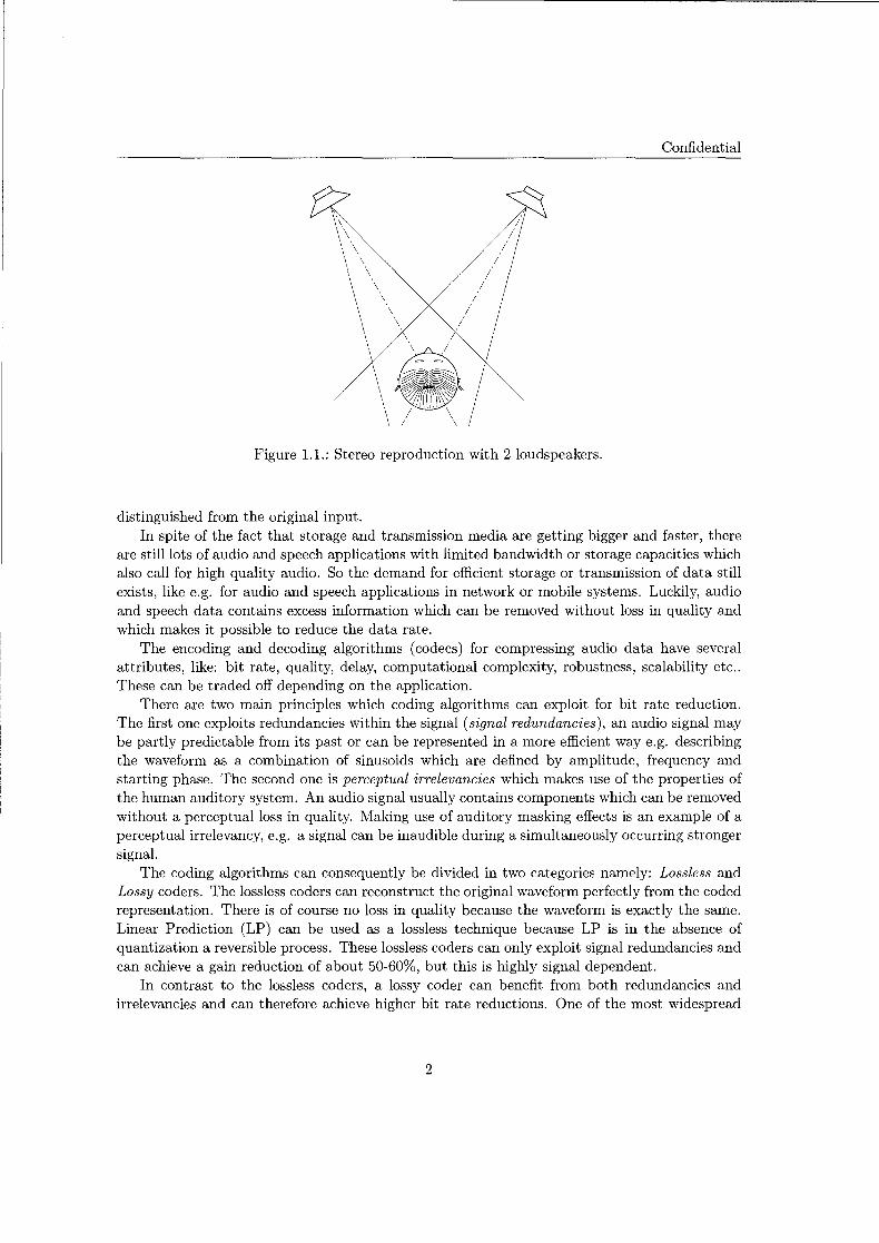
But these spatial cues are no longer present in a monophonic reproduction. Hence, stereophonic reproduction and of course recording methods were developed for trying to recreate the spatial sound image, similar to the live listening experience. The term stereophonic is derived from two Greek words: stereo, which means solid and implies multiple dimensions, and phonics, which means the science of sound. In the 1930's, Blumlein from Thorn E.M.I. and Fletcher et al. from Bell Laboratories independently did most of pioneering work for stereophonic recording and reproduction techniques [14]. For the reproduction of these early stereophonic sound multiple loudspeakers were used, ranging from 2 up to 80 (Flechter's wall of sound used an array of 80 microphones each connected to a corresponding loudspeaker, placed in an identical position, in a separate room). The movie industry applied the stereo sound in the 1960, and pushed the multichannel sound into the home market. Stereo is currently a widely accepted contraction of stereophonic, which generally refers to two-channel systems (see Fig. 1.1). Also headphones were used for reproduction and this is then called binaural or biphonic listening. An advantage of using headphones is that it is easier to control the received sound for the ears independently; with loudspeakers this left-right integrity of sound is not guaranteed.
The stereo sound was introduced and matured during the analog era, but since the introduction of the Compact Disc (CD) in the 1980's the recording and reproduction of wide-band audio has been shifted from the analog to the digital form. Nowadays the presence of the CD is ubiquitous. This digital form has quite some advantages over the analog way, like: high fidelity audio, a big dynamic range and its robustness. To represent the audio in digital format, quantization (subdivision into small but measurable increments for discrete moments in time) is needed and thus noise is introduced. To make the quantization noise inaudible, a sample frequency of 44.1 kHz was chosen at a resolution of 16 bits per sample which are coded with PCM. Because the CD mostly contains stereo audio, this results in a total bit rate of 44100 x 16 x 2 = 1411200 bits/sec. For some applications this high bit rate is an obstacle. The audio quality of the CD is considered to be transparent which means that the reconstructed audio output cannot be
1
Confidential
Figure 1.1.: Stereo reproduction with 2 loudspeakers.
distinguished from the original input. In spite of the fact that storage and transmission media are getting bigger and faster, there
are still lots of audio and speech applications with limited bandwidth or storage capacities which also call for high quality audio. So the demand for efficient storage or transmission of data still exists, like e.g. for audio and speech applications in network or mobile systems. Luckily, audio and speech data contains excess information which can be removed without loss in quality and which makes it possible to reduce the data rate.
The encoding and decoding algorithms ( codecs) for compressing audio data have several attributes, like: bit rate, quality, delay, computational complexity, robustness, scalability etc .. These can be traded off depending on the application.
There are two main principles which coding algorithms can exploit for bit rate reduction. The first one exploits redundancies within the signal (signal redundancies), an audio signal may be partly predictable from its past or can be represented in a more efficient way e.g. describing the waveform as a combination of sinusoids which are defined by amplitude, frequency and starting phase. The second one is perceptual irrelevancies which makes use of the properties of the human auditory system. An audio signal usually contains components which can be removed without a perceptual loss in quality. Making use of auditory masking effects is an example of a perceptual irrelevancy, e.g. a signal can be inaudible during a simultaneously occurring stronger signal.
The coding algorithms can consequently be divided in two categories namely: Lossless and Lossy coders. The lossless coders can reconstruct the original waveform perfectly from the coded representation. There is of course no loss in quality because the waveform is exactly the same. Linear Prediction (LP) can be used as a lossless technique because LP is in the absence of quantization a reversible process. These lossless coders can only exploit signal redundancies and can achieve a gain reduction of about 50-60%, but this is highly signal dependent.
In contrast to the lossless coders, a lossy coder can benefit from both redundancies and irrelevancies and can therefore achieve higher bit rate reductions. One of the most widespread
2
Confidential Chapter 1. Introduction
lossy coding standards for digital audio encoding is the MPEG-1 layer III standard, generally referred to as MP3. The achieved gain of these lossy coders is about 90%, e.g. MP3 can reduce a PCM file with a size of 40 megabyte to a 4 megabyte file. This makes them useful for network based applications. Lossy coders mainly depend on a psychoacoustic model which is based on knowledge of the human auditory system.
Since audio signals usually consist of at least two channels, which are supposed to be often related in some way, it may also be worthwhile to make use of inter-channel redundancies and irrelevancies. In [1] however is stated that there is not much correlation between the channels in the (short-term) time domain. But it can be easily shown that when recording a single sound source with a simple stereo microphone, the channels are related by their transfer functions. The cross-correlation in the frequency domain, therefore, shows more dependencies, especially the magnitudes of of the spectral coefficients [2]. However with the current digital mixing methods it is also easily feasible to create an artificial or synthetic stereo audio signal between which no cross-channel correlation is guaranteed.
There are already techniques which exploit cross-channel redundancies and/or irrelevancies, and these will be discussed later on in this report. But these techniques do not meet the desired criteria, hence this project was started.
1.1. Problem description and statement
This graduation project is done within the coding cluster of the DSP group from Philips Research Laboratories Eindhoven. The context of this is project is stereo coding. Stereo coding aims at removing redundancy and irrelevancy from the stereo signal to attain lower bit rates than the sum of the bit rates of the independently coded channels while maintaining the same quality level. Some known stereo coding techniques, which are briefly described in section 2.2, are: mid/side stereo coding, intensity coding, rotators over the total band or per frequency band, and parametric stereo coding. The most promising technique appears to be parametric stereo coding, it outperforms standard solutions like mid/side and intensity stereo coding. A problem with this coding is that the original signal can not be reconstructed perfectly due to the used perceptual model.
This brings us to the problem statement of this thesis: We desire a stereo coding technique subject to the following criteria:
1. Encoder and decoder form a system allowing perfect signal reconstructing in the absence of signal quantization and, thus, near perfect signal reconstruction at the high bit rate end.
2. The encoder constructs a main and a side signal similar to those provided by parametric perceptual stereo coding since this is advantageous for low bit rate coding purposes.
We propose to use a technique which is able to meet these constrains namely Linear Predictive Coding (LPC), based on FIR or IIR-filtering, in combination with a single rotator. LPC is able to reduce the redundancy in stereo signals and it is able to reconstruct the original perfectly, in the absence of quantization. It is also an often employed tool in audio and speech coding
3

1.2. Outline of this report Confidential
but not widely used for stereo coding. In the proposed system LPC is combined with a single rotator for constructing the main and the side signal, like in parametric stereo coding.
The objective of this thesis is: to see if it is feasible to extend or adapt known linear prediction techniques, as already used in speech and audio coding, to a two-channel system, and pinpointing possible problem areas. Furthermore, a very low bit rate is required to successfully compete with the current state-of-the-art stereo audio coders. Therefore experiments have to be performed to examine if low bit rates are achievable with the proposed system. There is even doubt [30] whether using LP is an efficient tool for stereo coding purposes.
1.2. Outline of this report
Chapter 2 provides some background information: a brief introduction into binaural perception and the origin of stereo signals. It furthermore describes the known stereo coding methods with their aims and shortcomings. Chapter 3 introduces the proposed Stereo Linear Prediction scheme with two different prediction filter implementations. In addition, methods are elaborated for optimizing the parameters of the proposed scheme. Finally some problem areas are stated with possible solutions. In chapter 4 existing one-channel LPC quantization schemes are described. Furthermore two preliminary ideas are proposed for quantization of the transmission coefficients. In chapter 5 an example is given to see if the results are in line with the expectations, and also some preliminary experiments which describe possible methods for bit rate reduction. Finally, in chapter 6 conclusions are drawn and some recommendation for future work are made.
4
2. Background
This chapter provides the reader with some background information desired for this thesis. The reader is assumed to be acquainted with linear prediction and rotation. If this is not the case an explanation can be found in appendix B and C.
This chapter, firstly, describes human sound perception, in particular the binaural perception, and the origin of the stereo signals. Secondly, known stereo coding methods are described detailing why they do not meet our demands.
2.1. Binaural perception and stereo signals
Binaural perception
Sound is the perception of air pressure variations picked up through our ears, and by using both ears (binaural) we are able to localize sound sources in 3 dimensional space. This perception of spatial sound(s) depends on the processing of spatial cues. The received sound waves travelled (slightly) different paths to both ears, due to the shape of the head and the position of the ears on the head. Therefore, the sound pressures reaching the ears are not entirely identical. From these differences, spatial cues can be extracted. Cues for spatial hearing can originate from:
• Intensity differences • Time differences • Interaural coherence • Pinnea • Head/Source Movement
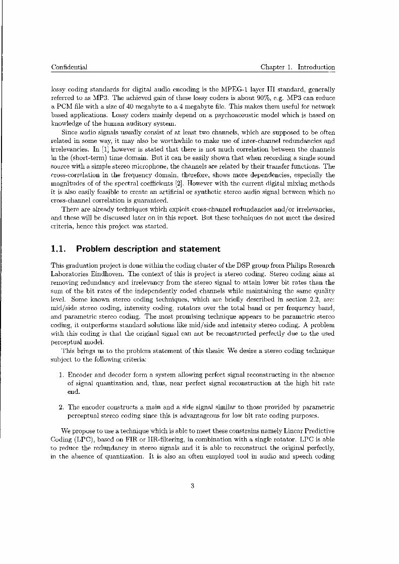
The Inter aural Intensity (or Level) Difference (liD) is related to the ratio of intensity of the sound pressures at both ears, the differences in intensity are mainly caused by the head. Sound coming from an off-centered source can vary in intensity in both ears due to the fact that the human head is an obstacle for the sound waves, therefore casts an acoustical shadow (Fig. 2.1), and thus the far ear receives less energy, the difference however is frequency and position dependent. At low frequencies liDs are insignificant, since the wavelength is much larger than the size of the head, and therefore these low frequencies do not cause large intensity differences (3dB for 500 Hz; 20dB for 6kHz). liDs due to propagational decay are usually less important than the decrease caused by the acoustic shadow, therefore only considerable for the more distant sound sources.
5

2.1. Binaural perception and stereo signals Confidential
Figure 2.1.: Acoustical shadow of the head at high frequencies.
For the same off-centered source, also the direct path for both ears differs in length, which results in a difference in time arrival. This is referred to Interaural Time Difference (lTD). For pure tones, this can be also be expressed as a phase difference (IPD). ITDs are dominant for frequencies below 1500 Hz. The ear which picks up the sound first determines the perceived direction of the sound (law of first wavefront or precedence effect). At the somewhat higher frequencies the human auditory system is not able to detect the fine-structure, however differences in the envelopes of the waveform can still be detected. For the pure tones, the maximum delay approaches at a phase lag of 180°, then the phase difference becomes ambiguous.
ITDs are not unique, i.e. multiple points in space have the same distances to both ears, thus giving the same lTD, and therefore causing a cone of confusion. Fortunately, other cues can resolve this ambiguity.
Not only the differences between both ears give spatial cues but also through similarities cues are obtained. Interaural Coherence (IC), defined as the overall similarity, can capture ambience properties (spatial diffuseness).
By using ITDs and liDs we can accurately localize sources in the horizontal plane (3.6° in front and 10° to the side [6]), but poorly in the median (vertical) plane. The sound perception in the median plane (vertical) differs because no time or intensity cues can aid in perception. However, changes in the spectrum are used, introduced through diffractions of pinnae and reflections from shoulder and torso. These are Head Related Transfer Functions, e.g. the pinnae can be seen as directional filter.
The previous cues are all static, i.e., it is assumed that listener and source have a fixed position in space. In practice, dynamic changes through head and/or source movement improve our source localizing (or tracking in case of source movement) capabilities and also resolve frontback ambiguity.
The human perceptive system is visual dominant, therefore sources can seem to emanate from a visual source, e.g., lips of a TV actor, rather than from the actual sound source, this is the so-called ventriloquist effect.
6
Confidential Chapter 2. Background
Stereophonic signals
The definition of stereophonic from the dictionary (Merriam-Webster) is: relating to, or constituting sound reproduction involving the use of separated microphones and two transmission channels to achieve the sound separation of a live hearing. In other words stereophonic is a way of recording and reproducing the sound will maintaining the complete spatial fidelity. However, Richard Heyser put this in a proper perspective by stating: "Stereo is merely an attempt to create the illusion of reality through the willing suspension of disbelief." [14].
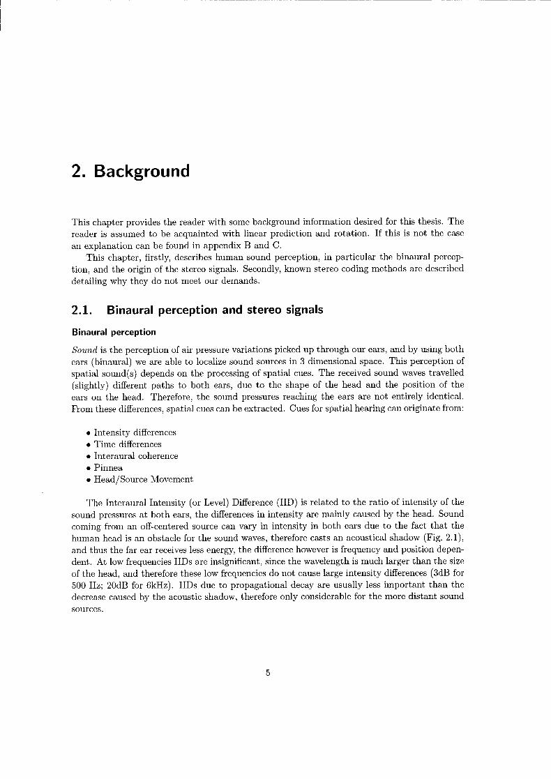
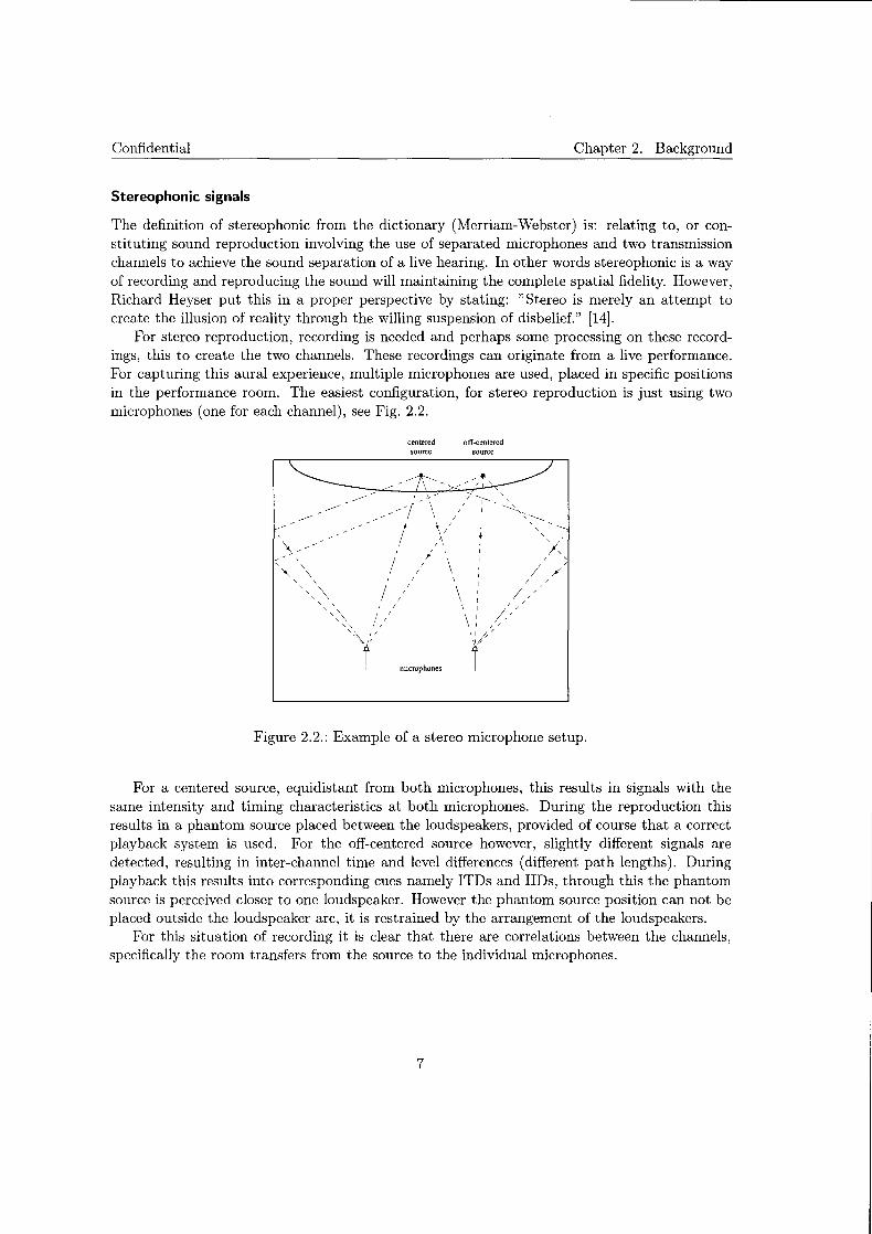
For stereo reproduction, recording is needed and perhaps some processing on these recordings, this to create the two channels. These recordings can originate from a live performance. For capturing this aural experience, multiple microphones are used, placed in specific positions in the performance room. The easiest configuration, for stereo reproduction is just using two microphones (one for each channel), see Fig. 2.2.
centered source
off-centered source
Figure 2.2.: Example of a stereo microphone setup.
For a centered source, equidistant from both microphones, this results in signals with the same intensity and timing characteristics at both microphones. During the reproduction this results in a phantom source placed between the loudspeakers, provided of course that a correct playback system is used. For the off-centered source however, slightly different signals are detected, resulting in inter-channel time and level differences (different path lengths). During playback this results into corresponding cues namely ITDs and liDs, through this the phantom source is perceived closer to one loudspeaker. However the phantom source position can not be placed outside the loudspeaker arc, it is restrained by the arrangement of the loudspeakers.
For this situation of recording it is clear that there are correlations between the channels, specifically the room transfers from the source to the individual microphones.
7

2.2. Stereo Coding Confidential
Another method for generating a stereo signal is by mixing pre-recorded (mono) signals. These can artificially be placed at different positions within the stereo image, by manipulating timing, intensity, reverberation etc. for both channels individually. For instance, a mono source can be panned by changing the intensity for both channels in a log and reverse-log manner [14]. A panoramic potentiometer (or pan pot in short) can be used for this artificially placing of different sources at different positions within the stereo image. By also introducing some timing differences a more natural spatial fidelity can be generated. This is of course a simple method for generating stereo signals, and a clear relation between channels exists.
However, practically mixing is more complex process where all kinds of technical considerations have to be taken into account, i.e which types of microphones to use, the placements of them, what is the goal for the reproduction: is it desired to re-create an sonic event or create a completely new one. Furthermore, different listener's perspectives are possible [14], i.e. "You are there" and "They are here" . With "You are there" the listener is transported into the same sonic environment as the event (the listener is put into the audience). With "They are here" it is attempted to bring the sonic event to the listener (the performers are put into the listener's room).
Some of these mixing methods, like creating a completely new event "where anything goes", can result in stereo signals with quite aribitrary relations between the channels.
2.2. Stereo Coding
Stereo coding aims at removing redundancies and irrelevancies from the stereo signal to attain lower bit rates than the sum of the separately coded channels, while maintaining the same quality level and preserving the spatial image. This is done by making use of the correlation between the channels or by exploiting binaural perceptual masking. The known stereo coding methods are:
• Sum Difference coding
• Intensity Stereo Coding
• Stereo Linear Prediction
• Complex Linear Prediction
• VECMA (Very Efficient Coding of Multichannel Audio)
• Parametric Stereo Coding
In the next subsections these techniques are briefly described with their advantages and shortcomings.
2.2.1. Sum-Difference coding
Sum-Difference coding, also known as Mid/Side coding, was first introduced by Johnston [25], as an extension to a transform coder. In this paper, it is proposed not to encode the left and
8
Confidential Chapter 2. Background
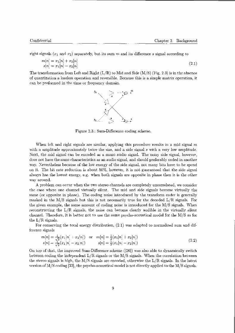
right signals (x1 and x2) separately, but its sum m and its difference s signal according to
m[n] = x1 [n] + x2[n] s[n] = x 1 [n] - x2[n] (2.1)
The transformation from Left and Right (1/R) to Mid and Side (M/S) (Fig. 2.3) is in the absence of quantization a lossless operation and reversible. Because this is a simple matrix operation, it can be preformed in the time or frequency domain.
m
a
x,
Figure 2.3.: Sum-Difference coding scheme.
When left and right signals are similar, applying this procedure results in a mid signal m
with a amplitude approximately twice the size, and a side signal s with a very low amplitude. Next, the mid signal can be encoded as a mono audio signal. The noisy side signal, however, does not have the same characteristics as an audio signal, and should preferably coded in another way. Nevertheless because of the low energy of the side signal, not many bits have to be spend on it. The bit rate reduction is about 50%, however, it is not guaranteed that the side signal always has the lowest energy, e.g. when both signals are opposite in phase then it is the other way around.
A problem can occur when the two stereo channels are completely uncorrelated, we consider the case where one channel virtually silent. The mid and side signals become virtually the same (or opposite in phase). The coding noise introduced by the transform coder is generally masked in the M/S signals but this is not necessarily true for the decoded 1/R signals. For the given example, the same amount of coding noise is introduced for the M/S signals. When reconstructing the 1/R signals, the noise can become clearly audible in the virtually silent channel. Therefore, it is better not to use the same psycho-acoustical model for the M/S as for the 1/R signals.
For conserving the total energy distribution, (2.1) was adapted to normalized sum and difference signals
m[n] = ~(x![n] + x2[n]) or m[n] = ~(x1[n] + x2[n]) s[n] = ~(xl[n]- x2[n]) s[n] = ~(xl[n]- x2[n])
(2.2)
On top of that, the improved Sum-Difference scheme ([26]) was also able to dynamically switch between coding the independent 1/R signals or the M/S signals. When the correlation between the stereo signals is high, the M/S signals are encoded, otherwise the 1/R signals. In the latest version of M/S coding [33], the psycho-acoustical model is not directly applied to the M/S signals.
g
2.2. Stereo Coding Confidential
2.2.2. Intensity stereo coding
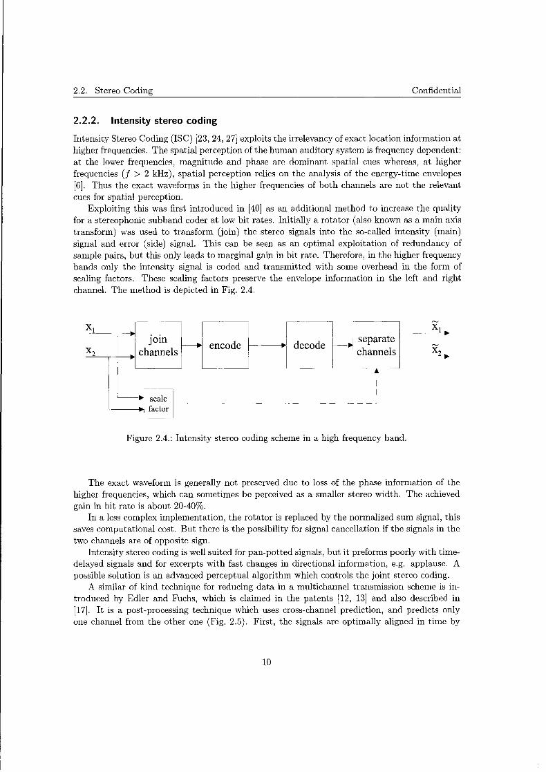
Intensity Stereo Coding (ISC) [23, 24, 27] exploits the irrelevancy of exact location information at higher frequencies. The spatial perception of the human auditory system is frequency dependent: at the lower frequencies, magnitude and phase are dominant spatial cues whereas, at higher frequencies (f > 2 kHz), spatial perception relies on the analysis of the energy-time envelopes [6]. Thus the exact waveforms in the higher frequencies of both channels are not the relevant cues for spatial perception.
Exploiting this was first introduced in [40] as an additional method to increase the quality for a stereophonic sub band coder at low bit rates. Initially a rotator (also known as a main axis transform) was used to transform (join) the stereo signals into the so-called intensity (main) signal and error (side) signal. This can be seen as an optimal exploitation of redundancy of sample pairs, but this only leads to marginal gain in bit rate. Therefore, in the higher frequency bands only the intensity signal is coded and transmitted with some overhead in the form of scaling factors. These scaling factors preserve the envelope information in the left and right channel. The method is depicted in Fig. 2.4.
XI
x2
_ .. ~
JOlll
channels
scale
~
~ enc ode
~·
decode J~ XI
t~~~::~ ~-------·-·~X~2 ..... ,---
1
I ~----
________________ j
Figure 2.4.: Intensity stereo coding scheme in a high frequency band.
The exact waveform is generally not preserved due to loss of the phase information of the higher frequencies, which can sometimes be perceived as a smaller stereo width. The achieved gain in bit rate is about 20-40%.
In a less complex implementation, the rotator is replaced by the normalized sum signal, this saves computational cost. But there is the possibility for signal cancellation if the signals in the two channels are of opposite sign.
Intensity stereo coding is well suited for pan-potted signals, but it preforms poorly with timedelayed signals and for excerpts with fast changes in directional information, e.g. applause. A possible solution is an advanced perceptual algorithm which controls the joint stereo coding.
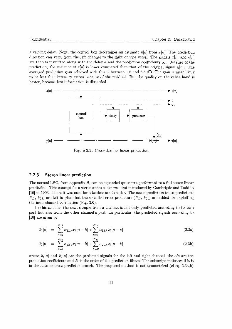
A similar of kind technique for reducing data in a multichannel transmission scheme is introduced by Edler and Fuchs, which is claimed in the patents [12, 13] and also described in [17]. It is a post-processing technique which uses cross-channel prediction, and predicts only one channel from the other one (Fig. 2.5). First, the signals are optimally aligned in time by
10
Confidential Chapter 2. Background
a varying delay. Next, the control box determines an estimate y[n] from x[n]. The prediction direction can vary, from the left channel to the right or vice versa. The signals x[n] and e[n] are then transmitted along with the delay d and the prediction coefficients ak. Because of the prediction, the variance of e[n] is lower compared than that of the original signal y[n]. The averaged prediction gain achieved with this is between 1.5 and 6.5 dB. The gain is most likely to be less than intensity stereo because of the residual. But the quality on the other hand is better, because less information is discarded.
x[n] --
~ x[n]
~- --~--~--~~~~-~-~· d -- - - - - ~ - - - - - - - - -- - - - - - - - - - - -· . ~
control 4 delay ______. predictor box
c--
---r-- 1\ ~ y[n]
+r-1\ ~\_ I_/ y[n] e[n]
Figure 2.5.: Cross-channel linear prediction.
2.2.3. Stereo linear prediction
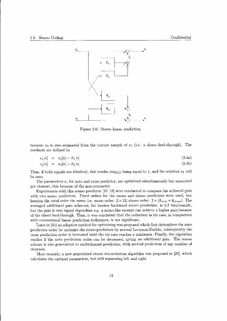
The normal LPC, from appendix B, can be expanded quite straightforward to a full stereo linear prediction. This concept for a stereo audio coder was first introduced by Cambrigde and Todd in [10] in 1993. There it was used for a lossless audio coder. The mono predictors (auto-predictors: P11 , P22) are left in place but the so-called cross-predictors (P12, P21) are added for exploiting the inter-channel correlation (Fig. 2.6).
In this scheme, the next sample from a channel is not only predicted according to its own past but also from the other channel's past. In particular, the predicted signals according to [10] are given by
N11 N~
L:an,kxl[n ~ k] + 'L:a12,kx2[n ~ k] (2.3a) k=l k=l N22 N21
L a22,kx2 [n ~ k] + L a21,kxl [n ~ k] (2.3b) k=l k=O
where x1 [n] and x2[n] are the predicted signals for the left and right channel, the a's are the prediction coefficients and N is the order of the prediction filters. The subscript indicates if it is in the auto or cross predictor branch. The proposed method is not symmetrical ( cf eq. 2.3a, b)
11
2.2. Stereo Coding Confidential
et +
" XI
+ +
--'x,:__ _ _j_ ________ _:r,+ffi-·______. e,
Figure 2.6.: Stereo linear prediction.
because x2 is also estimated from the current sample of x1 (i.e., a direct feed-through). The residuals are defined by
x1 [n] - ::h [n]
x2[n]- x2[n]
(2.4a)
(2.4b)
Thus, if both signals are identical, this results ina21,0 being equal to 1, and the residual e2 will be zero.
The parameters a, for auto and cross predictor, are optimized simultaneously but separated per channel, this because of the non-symmetry.
Experiments with this stereo predictor [10, 18] were conducted to compare the achieved gain with two mono predictors. Fixed orders for the mono and stereo predictors were used, but keeping the total order the same, i.e. mono order: 2 X 12; stereo order: 2 X (8auto + 4cross)· The averaged additional gain achieved, for lossless backward stereo prediction, is 0.3 bits/sample, but the gain is very signal dependent e.g. a mono-like excerpt can achieve a higher gain because of the direct feed-through. Thus, it was concluded that the reduction in bit rate, in comparison with conventional linear prediction techniques, is not significant.
Later in [31] an adaptive method for optimizing was proposed which first determines the auto prediction order by optimize the mono predictors by normal Levinson-Durbin, subsequently the cross prediction order is increased until the bit rate reaches a minimum. Finally, the algorithm verifies if the auto prediction order can be decreased, giving an additional gain. The stereo scheme is also generalized to multichannel prediction, with mutual prediction of any number of channels.
More recently, a new generalized stereo decorrelation algorithm was proposed in [20], which calculates the optimal parameters, but still separating left and right.
12
Confidential Chapter 2. Background
Finally, in [19] block Levinson [36] is proposed for the non-direct feed-trough branch, under the restriction of equal orders Nu = N12· In here, also forward adaption is compared with backward adaptation. Backward adaptation is used, such that no parameters a have to be transmitted. A proper method for quantizing these coefficients is not known.
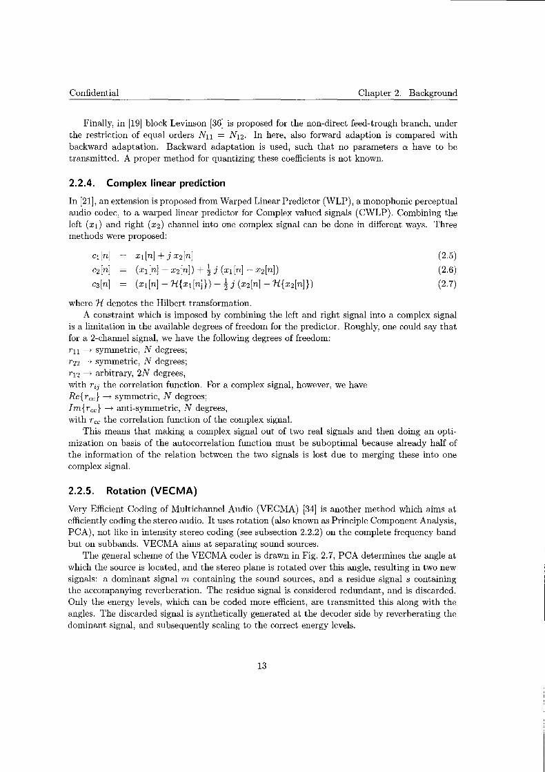
2.2.4. Complex linear prediction
In [21], an extension is proposed from Warped Linear Predictor (WLP), a monophonic perceptual audio codec, to a warped linear predictor for Complex valued signals (CWLP). Combining the left (xl) and right (x2) channel into one complex signal can be done in different ways. Three methods were proposed:
x1[n] + j x2[n]
(xl[n] + x2[n]) + ~ j (xl[n] - x2[n])
(x1[n]-1i{x1[n]}) + ~ j (x2[n]-1i{x2[n]})
where 1i denotes the Hilbert transformation.
(2.5)
(2.6)
(2.7)
A constraint which is imposed by combining the left and right signal into a complex signal is a limitation in the available degrees of freedom for the predictor. Roughly, one could say that for a 2-channel signal, we have the following degrees of freedom: ru ----+ symmetric, N degrees; r22 ----+ symmetric, N degrees; r12 ----+ arbitrary, 2N degrees, with Tij the correlation function. For a complex signal, however, we have Re{ree}----+ symmetric, N degrees; Im{ree}----+ anti-symmetric, N degrees, with Tee the correlation function of the complex signal.
This means that making a complex signal out of two real signals and then doing an optimization on basis of the autocorrelation function must be suboptimal because already half of the information of the relation between the two signals is lost due to merging these into one complex signal.
2.2.5. Rotation (VECMA)
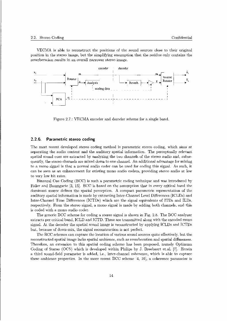
Very Efficient Coding of Multichannel Audio (VECMA) [34] is another method which aims at efficiently coding the stereo audio. It uses rotation (also known as Principle Component Analysis, PCA), not like in intensity stereo coding (see subsection 2.2.2) on the complete frequency band but on subbands. VECMA aims at separating sound sources.
The general scheme of the VECMA coder is drawn in Fig. 2. 7, PCA determines the angle at which the source is located, and the stereo plane is rotated over this angle, resulting in two new signals: a dominant signal m containing the sound sources, and a residue signal s containing the accompanying reverberation. The residue signal is considered redundant, and is discarded. Only the energy levels, which can be coded more efficient, are transmitted this along with the angles. The discarded signal is synthetically generated at the decoder side by reverberating the dominant signal, and subsequently scaling to the correct energy levels.
13
2.2. Stereo Coding Confidential
VECMA is able to reconstruct the positions of the sound sources close to their original position in the stereo image, but the simplifying assumption that the residue only contains the reverberation results in an overall narrower stereo image.
XI
x,
------
_ _______. III
Rotator rS-..
I I I I
PCA _C!.L----
encoder decoder
~Reverb. m~·-·---:r----··l>x1
Inverse
1--~{:;>--s Rotator .,. x,
I :6;
~Analysis I ; scaling data I --------~-----------
1 I
-----------~-------------------•
I I
Figure 2.7.: VECMA encoder and decoder scheme for a single band.
2.2.6. Parametric stereo coding
The most recent developed stereo coding method is parametric stereo coding, which aims at separating the audio content and the auditory spatial information. The perceptually relevant spatial sound cues are extracted by analyzing the two channels of the stereo audio and, subsequently, the stereo channels are mixed down to one channel. An additional advantage for mixing to a mono signal is that a normal audio coder can be used for coding this signal. As such, it can be seen as an enhancement for existing mono audio codecs, providing stereo audio at low to very low bit rates.
Binaural Cue Coding (BCC) is such a parametric coding technique and was introduced by Faller and Baumgarte [3, 15]. BCC is based on the assumption that in every critical band the dominant source defines the spatial perception. A compact parametric representation of the auditory spatial information is made by extracting Inter-Channel Level Differences (ICLDs) and Inter-Channel Time Differences (ICTDs) which are the signal equivalents of ITDs and ILDs, respectively. From the stereo signal, a mono signal is made by adding both channels, and this is coded with a mono audio coder.
The generic BCC scheme for coding a stereo signal is shown in Fig. 2.8. The BCC analyzer extracts per critical band, ICLD and ICTD. These are transmitted along with the encoded mono signal. At the decoder the spatial sound image is reconstructed by applying ICLDs and ICTDs but, because of down-mix, the signal reconstruction is not perfect.
The BCC schemes can capture the location of various sound sources quite effectively, but the reconstructed spatial image lacks spatial ambience, such as reverberation and spatial diffuseness. Therefore, an extension to this spatial coding scheme has been proposed, namely Optimum Coding of Stereo (OCS) which is developed within Philips by J. Breebaart et.al. [7]. Herein a third sound-field parameter is added, i.e., inter-channel coherence, which is able to capture these ambience properties. In the more recent BCC scheme [4, 16], a coherence parameter is
14

Confidential Chapter 2. Background
also included.
down mix
encoder decoder
BCC side information -------t----------------,
I I
audio encoder
I I I audio BCC
decoder synthesis
Figure 2.8.: Generic Binaural Cue Coding scheme.
X:, ...
The OCS scheme is generally the same as BCC (Fig. 2.8), the parameters are extracted from the stereo signal. The power ratio of the corresponding subband b is defined as
with X the DFT of signal x and where the summations extend over all k's within the sub band b. The inter-channel phase difference is obtained as follows
(2.9)
The inter-channel coherence is defined as
(2.10)
with X1 and X2 the DFT of the signals after phase alignment according to the estimated IPD. Next to the additional IC parameter, another difference with the BCC scheme is that the
down-mix is more refined. Furthermore, an Overall Phase Difference (OPD) is transmitted which enables reconstructing with the proper alignment,
The parameters are quantized according to their perceptual relevance, e.g., the IPD are not relevant for higher frequencies and are only transmitted for frequency bands up to about 2 kHz. The parameter bit rate is estimated at 7. 7 kbitsjsec, this is the additional bit rate needed to extend a mono to a stereo signal using OCS. This bit rate can be decreased further when by reducing the number of frequency bands (1 kbit/sec), thus achieving very low bit rates. Notwithstanding this success of OCS for the low bit rates, it appears to be difficult to attain transparency at high bit rates when using this technique. This is presumably due to the imposed model.
15

2.2. Stereo Coding Confidential
16
3. Stereo LPC
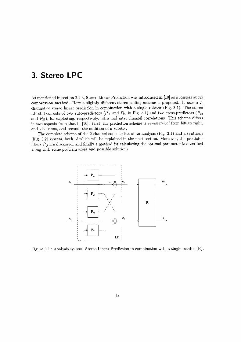
As mentioned in section 2.2.3, Stereo Linear Prediction was introduced in [10] as a lossless audio compression method. Here a slightly different stereo coding scheme is proposed. It uses a 2-channel or stereo linear prediction in combination with a single rotator (Fig. 3.1). The stereo LP still consists of two auto-predictors (Pn and P22 in Fig. 3.1) and two cross-predictors (P12 and P21), for exploiting, respectively, intra and inter channel correlations. This scheme differs in two aspects from that in [10]. First, the prediction scheme is symmetrical from left to right, and vice versa, and second, the addition of a rotator.
The complete scheme of the 2-channel co dec exists of an analysis (Fig. 3.1) and a synthesis (Fig. 3.2) system, both of which will be explained in the next section. Moreover, the predictor filters Pij are discussed, and finally a method for calculating the optimal parameter is described along with some problem areas and possible solutions.
-----------------------'
m ..
R
+ s
LP
Figure 3.1.: Analysis system: Stereo Linear Prediction in combination with a single rotator (R).
17

3.1. Two-channel LP and rotation Confidential
3.1. Two-channel LP and rotation
In this section, we describe the stereo LP analysis and synthesis and rotation systems.
Analysis system
The analysis system, or encoder, (Fig. 3.1) exist of two basic blocks, namely a stereo linear predictor and a rotator (R).
The Stereo Linear Predictor removes redundancies which are present in the input signals (x1
and x2), by making estimate signals ::h and x2 from the previous (filtered) samples of x1 and x 2 . The estimation for the left and right channel is abstractly given by
Na Nc
xl[n] = L an,kYl,k[n] + L a12,kY2,k[n] (3.1a)
k=l k=l
Nc Na
x2[n] = L a21,kYl,k[n] + L a22,kY2,k[n] (3.1b)
k=l k=l
with prediction coefficients aij,k (i,j = 1,2), auto prediction order Na, cross order Nc and the weighted input signals Yi,k = fk *Xi, where fk are the impulse responses of causal stable filters with no direct feed-through. The summations with coefficients an and a22 indicate the autopredictors, and the summations with coefficients a12 and a21 the cross-predictors. So unlike the scheme in [10], no direct feed-through is used.
The residual or prediction errors ( e1 and e2) originate from subtracting the estimated signals from the original ones:
Na Nc
e1 [n] = x1 [n] - x1 [n] = x1 [n] - L an,kYl,k [n] - L a12,kY2,k [n], (3.2a) k=l k=l
Nc Na
e2[n] = x2[n]- x2[n] = x2[n]- L a21,kYl,k[n]- L a22,kYl,k[n]. (3.2b) k=l k=l
In vector notation, and with the condition of equal orders i.e. Na = Nc = N, this can be written
as
N N , "'"' [ xl[n] ] "'"' [ an k f.[n] = !f.[n] - !!;_[n] = !f.[n] - L....- Ak~[n] = x [n] - L..._.- a '
k=l 2 k=l 21,k ] [
Yl,k [n] ] (3.3) Y2,k[n]
Transformed to frequency domain this will result in
E(z) = H(z). X(z) = [ 1- Pn(z) -P12(z) ] [ X1(z) ] - - -P21(z) 1- P22(z) X2(z)
(3.4)
18
Confidential Chapter 3. Stereo LPC
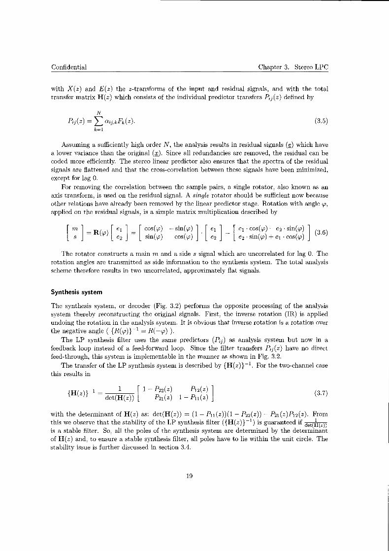
with X(z) and E(z) the z-transforms of the input and residual signals, and with the total transfer matrix H( z) which consists of the individual predictor transfers Pij ( z) defined by
N
Pij(z) = L aij,kFk(z). (3.5) k=1
Assuming a sufficiently high order N, the analysis results in residual signals (~) which have a lower variance than the original (;r,). Since all redundancies are removed, the residual can be coded more efficiently. The stereo linear predictor also ensures that the spectra of the residual signals are flattened and that the cross-correlation between these signals have been minimized, except for lag 0.
For removing the correlation between the sample pairs, a single rotator, also known as an axis transform, is used on the residual signal. A single rotator should be sufficient now because other relations have already been removed by the linear predictor stage. Rotation with angle r.p, applied on the residual signals, is a simple matrix multiplication described by
- sin(r.p) ] . [ e1 ] = [ e1 · cos(r.p)- e2 · sin(r.p) ] (3.6) cos(r.p) e2 e2 · sin(r.p) + e1 · cos(r.p)
The rotator constructs a main m and a side s signal which are uncorrelated for lag 0. The rotation angles are transmitted as side information to the synthesis system. The total analysis scheme therefore results in two uncorrelated, approximately flat signals.
Synthesis system
The synthesis system, or decoder (Fig. 3.2) performs the opposite processing of the analysis system thereby reconstructing the original signals. First, the inverse rotation (IR) is applied undoing the rotation in the analysis system. It is obvious that inverse rotation is a rotation over the negative angle ( { R( r.p)} - 1 = R( -r.p) ).
The LP synthesis filter uses the same predictors ( Pij) as analysis system but now in a feedback loop instead of a feed-forward loop. Since the filter transfers Pij(z) have no direct feed-through, this system is implementable in the manner as shown in Fig. 3.2.
The transfer of the LP synthesis system is described by {H(z)} - 1. For the two-channel case this results in
-1 1 [ 1 - p22 ( z) {H(z)} = det(H(z)) P21(z)
P12(z) ] 1- Pn(z)
(3.7)
with the determinant of H(z) as: det(H(z)) = (1- Pn(z))(1- P22(z))- P21(z)P12(z). From this we observe that the stability of the LP synthesis filter ( {H(z)} - 1) is guaranteed if det(i:J(z))
is a stable filter. So, all the poles of the synthesis system are determined by the determinant of H(z) and, to ensure a stable synthesis filter, all poles have to lie within the unit circle. The stability issue is further discussed in section 3.4.
19
3.2. Prediction filters Confidential
--------'
m
IR
: LP' L ______________________ I
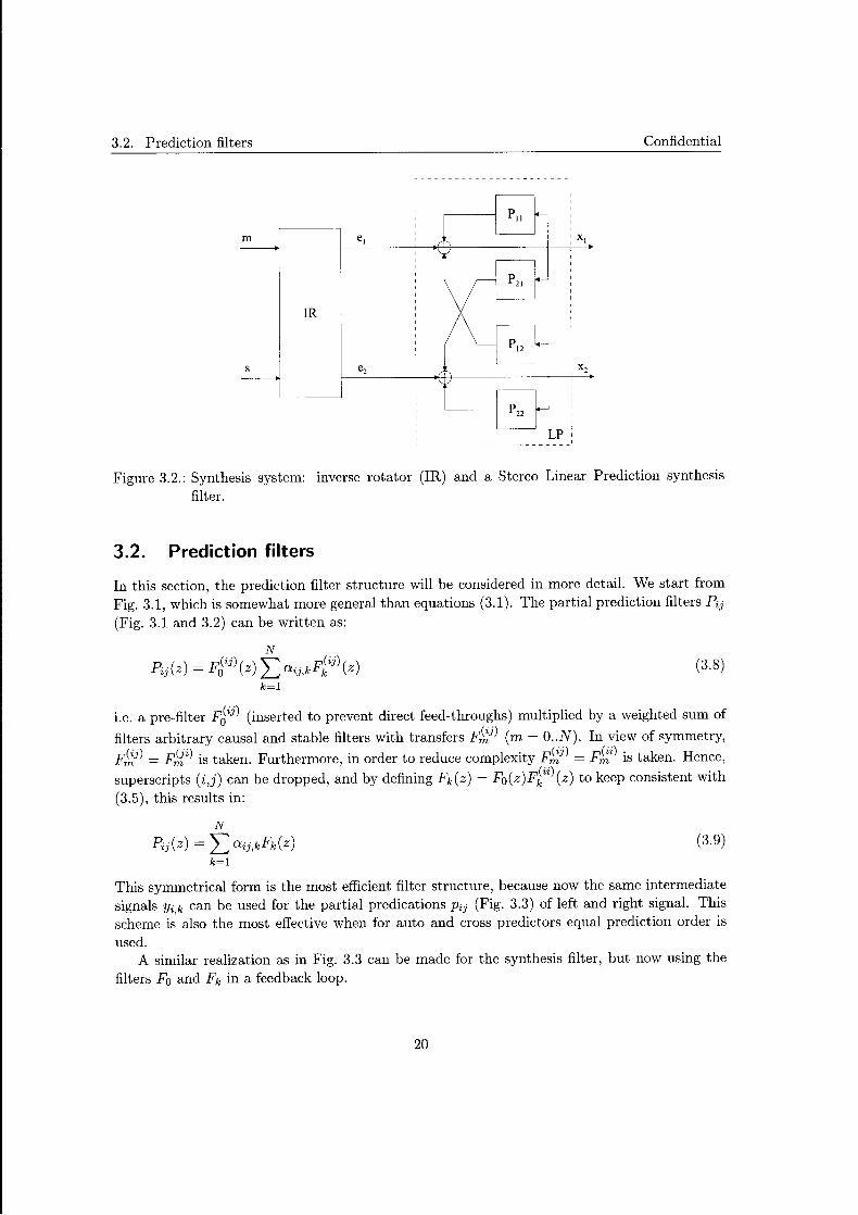
Figure 3.2.: Synthesis system: inverse rotator (IR) and a Stereo Linear Prediction synthesis filter.
3.2. Prediction filters
In this section, the prediction filter structure will be considered in more detail. We start from Fig. 3.1, which is somewhat more general than equations (3.1). The partial prediction filters Pij (Fig. 3.1 and 3.2) can be written as:
N (ij) (ij)
Pij(z) =Fa (z) 2::::a~ij,kFk (z) (3.8) k=l
i.e. a pre-filter FJij) (inserted to prevent direct feed-throughs) multiplied by a weighted sum of
filters arbitrary causal and stable filters with transfers F!:;j) (m = O .. N). In view of symmetry,
F!:;j) = F/r{i) is taken. Furthermore, in order to reduce complexity F!:;j) = F!:;i) is taken. Hence,
superscripts (i,j) can be dropped, and by defining Fk(z) = Fa(z)Fkii)(z) to keep consistent with (3.5), this results in:
N
Pij(z) = L O:ij,kFk(z) (3.9) k=l
This symmetrical form is the most efficient filter structure, because now the same intermediate signals Yi,k can be used for the partial predications Pij (Fig. 3.3) of left and right signal. This scheme is also the most effective when for auto and cross predictors equal prediction order is used.
A similar realization as in Fig. 3.3 can be made for the synthesis filter, but now using the filters Fa and Fk in a feedback loop.
20

Confidential Chapter 3. Stereo LPC
+
Figure 3.3.: Symmetrical filter implementation of a two-channel analysis predictor.
21
3.3. Calculation of the optimal parameters Confidential
The simplest choice for Fk(z) would be to use a Tapped-Delay-Line (TDL) as filter structure, i.e., Fk(z) = z-k. In this case (3.4) can be rewritten, using (3.9) and the TDL transfer, to a compact notation
N N ~[n] = L A~O£[n] or as transfer H(z) = L A~z-k (3.10)
k=O k=O
with A~= I= [ ~ ~ ] and A~= -Ai fori= l..N, still assuming equal orders (Na = Nc = N). From [8, 22], we know that for audio signals it is advantageous to take a warped filter struc
ture, according to a psycho-acoustical frequency scale (e.g. the Bark Scale) by using Laguerre filters. In the case of Laguerre filters, the filters Fk are given by
- -1 ,11- A2 (-A+ z-1)k-1 Fk(z)- z 1- z-1A 1- Az-1 (3.11)
with Laguerre coefficient IAI < 1. A warping factor A= 0.7564 (for sample frequency Fs = 44.1 kHz) gives a good correspondence to a Bark scale [39]. Performing LP on this warped scale places more emphasizes on accurate modelling of the spectral envelope of the input signal at the lower frequencies. A= 0 results in a TDL, like discussed above.
For the Laguerre system, the resulting transfer is given by
(3.12)
Conform [8], this expression can be rewritten to an all-pass line with the following notation
(3.13)
with a linear mapping from Ak to Bk.
3.3. Calculation of the optimal parameters
The outputs of the analysis system, as depicted in Fig. 3.1, are the main m and side s signal. Optimizing the parameters, i.e., the prediction coefficients and rotation angle, can be defined as an optimization problem which produces a maximum of a squared sum of the main signal (max {I:nlm[n]l 2} ), which automatically induces a minimum for the squared sum of the side signal (min {I:nls[n]i2} ).
It can be proved (see appendix E) that joint optimization of prediction coefficients a's and rotation angle r.p is equal to sequential optimization of a's based on minimization of the squared sum of the residual signals (min{I:nle1[n]l 2} and min{I:nle2[n]i2}), followed by PCA on the residuals e1 and e2. The calculation of the optimal prediction coefficients is now considered in more detail.
22
Confidential Chapter 3. Stereo LPC
Optimal stereo-LPC coefficients
For calculation of the optimal stereo LP coefficients, we can consider min {~nlel[n]i2} where er is determined by coefficients an,k, fork= l..Na, and a 12,k, fork= l..Nc. For convenience we introduce the following vectors:
[ei[O], ei[1], · · · , ei[L]]t for i = 1, 2,
[xi[ OJ, xi[1], · · · , xi[L]]t for i = 1, 2,
Yi,k [Yi,k[O], Yi,k[1], · · · , Yi,k[L]]t for i = 1, 2 and k = 1, · · · , max(Na, Nc)
(3.14)
(3.15)
(3.16)
with data length L, and
[aii,l, aii,2, , aii,Nalt for i = 1, 2
[aij,l, aij,2, · · · , aij,NJ for i, j = 1, 2 and i-!=- j.
Furthermore, we introduce the matrices Yi ( i, 1, 2) by
[771,1, Y1,2,
[Yi,l, Y1,2,
Yl,Na' Y2,1, Y2,2,
Yl,Ncl Y2,1, fh,2,
From the previous definitions, it follows that
l Y2,Nc] l
' Y2,Nal·
where [ Qn ] is a stacked vector of auto and cross prediction coefficients. Q12
a, is given by the normal equations
(3.17)
(3.18)
(3.19)
(3.20)
(3.21)
Thus, the optimal
(3.22)
From minimizing ~nle~[n]l, a similar normal equation can be obtained for the remaining coeffcients:
(3.23)
Calculation of the optimal a's can be done by directly solving these two sets of normal equations ((3.22) and (3.23)), but this is not always the most efficient way. For the condition of equal order Na = Nc = N, we have that Y1 = Y2 = Y resulting in the following set of equations
(3.24)
23
3.3. Calculation of the optimal parameters Confidential
For equal order, the square matrix yty consists of 4 Toeplitz matrices:
Rn,o Rn,-1 Rn,-(N-1) R21,o R21,-1
Rn,1 Rn,o Rn,-(N-2) R21,1 R21,o
yty= Rn,N-1 Rn,N-2 Rn,o R21,1 R21,o
R12,o R12,-1 R12,-(N-1) R22,o R22,-1
R12,1 R12,o R12,-(N-2) R22,1 R22,o
R12,N-1 R12,N-2 R12,o R22,1 R22,o
with
N-1
Rij,k = 2:: yi[n]yj[n + k] k=-(N-1)
R21,-(N-1)
R21,-(N-2)
R22,-(N-1)
R22,-(N-2)
If we now define a 2 x 2 block matrix (is not necessarily a Toeplitz), as
Rk = [ Rn,k R12,k ] R21,k R22,k
the matrix yty can be reorganized into a block- Toeplitz structure according to
Ro R-1 R-2 R-(N-1) Rt Ro R-1 R-(N-2) R2 Rt Ro R-(N-3)
RN-1 RN-2 RN-3 Ro
(3.25)
(3.26)
(3.27)
(3.28)
Symmetry of block-Toeplitz matrix is not guaranteed because Rk = R_kt but generally not
Rk #- R-k· The normal equation (3.24) can thus be written as
Ro · R_t R-2 R-N+l At Yt Rt Ro R-1 R-N+2 A2 Y2 Rt R2 Ro R-N+3 A3 Y3 (3.29)
RN-1 RN-2 RN-3 Ro AN YN
with equal-sized square matrices Rk, Ak and Yk, and where the prediction coefficients Ak are the unknowns to be solved. An iterative Levinson [37] type of algorithm can be used, namely the block-Levinson algorithm by Wiggins and Robinson (also known as Levinson-(Whittle)Wiggins-Robinson or LWR algorithm [41, 36]) which is an efficient way for solving this.
A difference with the normal (one-channel) Levinson algorithm is that, in the multichannelcase, matrix operations appear and special care has to be taken since matrix multiplications
24
Confidential Chapter 3. Stereo LPC
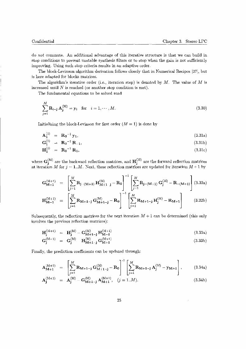
do not commute. An additional advantage of this iterative structure is that we can build in stop conditions to prevent unstable synthesis filters or to stop when the gain is not sufficiently improving. Using such stop criteria results in an adaptive order.
The block-Levinson algorithm derivation follows closely that in Numerical Recipes [37], but is here adapted for blocks matrices.
The algorithm's iterative order (i.e., iteration step) is denoted by M. The value of M is increased until N is reached (or another stop condition is met).
The fundamental equations to be solved read
M
LRi-j AJM) = Yi for i = 1, · · ·, M. j=1
Initializing the block-Levinson for first order (M = 1) is done by
A(1) 1
G(1) 1
H(1) 1
Ro-1 Y1>
Ro- 1 R-1,
Ro - 1 R1,
(3.30)
(3.31a)
(3.31b)
(3.31c)
where GjM) are the backward reflection matrices, and HjM) are the forward reflection matrices at iteration M for j = l..M. Next, these reflection matrices are updated for iteration M + 1 by
[ t, RJ-(M+l) H~~l-j - II, r 1
[t, Rj-(M+l) GjMl - R-(M+l) l (3.32a)
[t,RM+l-J G~~l-j- 11,]-l [t,RM+l-j HjMl- RM+ll (3.32b)
Subsequently, the reflection matrices for the next iteration M + 1 can be determined (this only involves the previous reflection matrices):
H~M+l) J
G~M+l) J
Finally, the prediction coefficients can be updated through:
A(M+l) M+1 [t RM+l-j G~l1-j - Ro]-
1 [t RM+1-j AJM) - YM+ll ]=1 J=1
(M) (M) (M+1) (. _ ) Aj - GM+l-j AM+l , J - l..M .
25
(3.33a)
(3.33b)
(3.34a)
(3.34b)
3.4. Practical problems and solutions Confidential
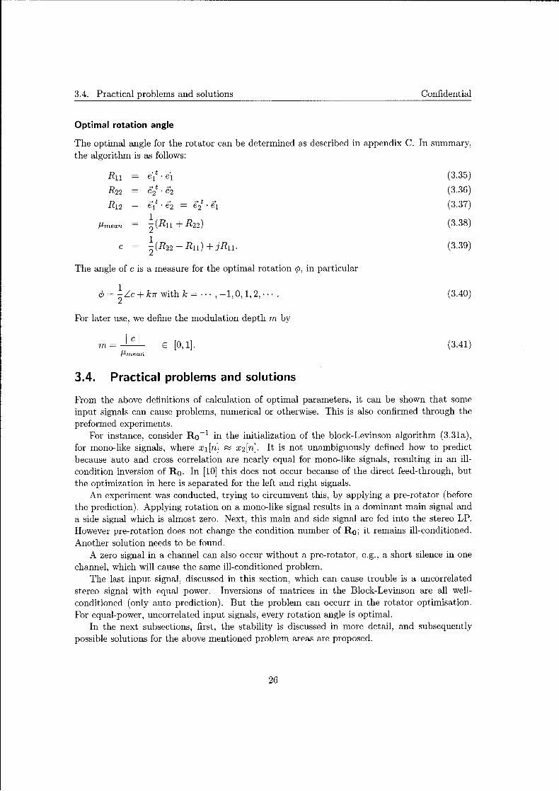
Optimal rotation angle
The optimal angle for the rotator can be determined as described in appendix C. In summary, the algorithm is as follows:
~t ~ e1 · e1 ~t ~ e2 · e2 -tt """'* -t -e1 · e2 e2 · e1
f..lrnean 1 "2(Rn + R22)
c ~(R22- Rn) + jRn.
The angle of c is a measure for the optimal rotation ¢, in particular
-+.=~L:c+brwithk=··· -1012 ··· '+' 2 ' ' ' ' ' .
For later use, we define the modulation depth m by
I c I m=--f..lrnean
E [0, 1].
3.4. Practical problems and solutions
(3.35)
(3.36)
(3.37)
(3.38)
(3.39)
(3.40)
(3.41)
From the above definitions of calculation of optimal parameters, it can be shown that some input signals can cause problems, numerical or otherwise. This is also confirmed through the preformed experiments.
For instance, consider Ro -l in the initialization of the block-Levinson algorithm (3.31a), for mono-like signals, where x1[n] ~ x2[n]. It is not unambiguously defined how to predict because auto and cross correlation are nearly equal for mono-like signals, resulting in an illcondition inversion of Ro. In [10] this does not occur because of the direct feed-through, but the optimization in here is separated for the left and right signals.
An experiment was conducted, trying to circumvent this, by applying a pre-rotator (before the prediction). Applying rotation on a mono-like signal results in a dominant main signal and a side signal which is almost zero. Next, this main and side signal are fed into the stereo LP. However pre-rotation does not change the condition number of R 0 ; it remains ill-conditioned. Another solution needs to be found.
A zero signal in a channel can also occur without a pre-rotator, e.g., a short silence in one channel, which will cause the same ill-conditioned problem.
The last input signal, discussed in this section, which can cause trouble is a uncorrelated stereo signal with equal power. Inversions of matrices in the Block-Levinson are all wellconditioned (only auto prediction). But the problem can occurr in the rotator optimisation. For equal-power, uncorrelated input signals, every rotation angle is optimal.
In the next subsections, first, the stability is discussed in more detail, and subsequently possible solutions for the above mentioned problem areas are proposed.
26

Confidential Chapter 3. Stereo LPC
3.4.1. Stability of the 2-channel synthesis filter
First of all, stability of the whole system is determined by the stability of the stereo synthesis LP filter, and the stability of this synthesis filter, as mentioned before, is determined by the roots of det(H(z)). This means that the synthesis system is stable if det(H(z)) #- 0 for lzl > 1.
According to Whittle [42], a stable solution is guaranteed when the block-Levinson algorithm is used. However, this algorithm only applies for equal orders of (Na = Nc) and gives no information concerning stability for unequal orders Na #- Nc (and Nc #- 0).
Experiments have been conducted, optimizing the system by solving the normal equations (3.22) and (3.23) for different orders. After analysis the prediction coefficients were examined, more specific the roots of the determinant of H ( z). Plotted in Fig. 3.4 is the maximum magnitude of these roots per frame. Fig. 3.4a depicts the result for order Na = Nc = 10, and the horizontal dashed line indicates the maximum for which stability of the synthesis filter is guaranteed. The experiment confirms that, for equal order, the synthesis filter is stable for all frames. In Fig. 3.4b the results are given for the case that Na = 10 and Nc = 3. It is clear that not in all frames a stable inverse system occurs.
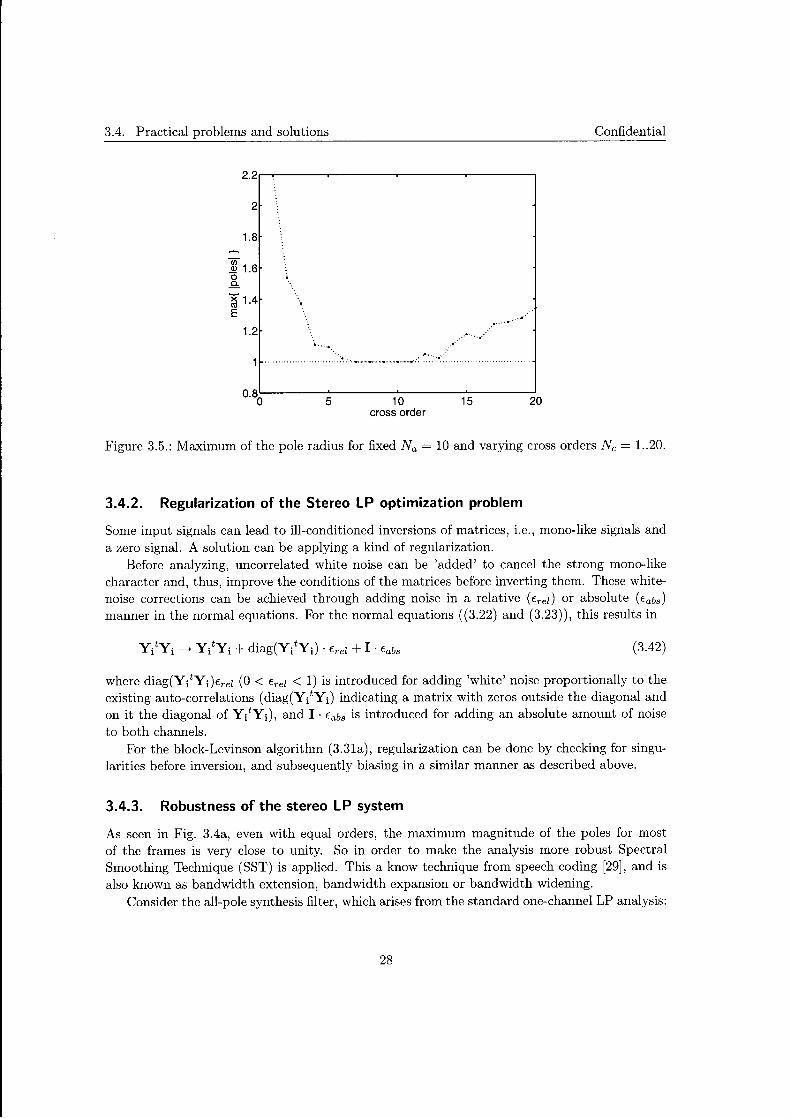
For experimentally finding the stable region, tests were preformed analyzing different excerpts with varying cross-prediction orders and a fixed auto prediction order [5]. Result are shown in Fig. 3.5 for Na = 10 and Nc = 1..20. For cross-orders of Nc = 7 until Nc = 11, a stable inverse system was found. However, such results are excerpt dependent, but all have the same trend, i.e., stable around the point of equal order and unstable regions before and after this point, where the width of stable region differs for various excerpts. We infer from this that stability of the synthesis filter can only be unconditionally guaranteed for Nc = 0 or Nc = Na.
0.8
-;j)
~ 0.6 ..£!,
x "' E 0.4
0.2
100 200 frame
(a)
300 400
1.4,....-------..-----;r----~------,
I o.8 0
..£!,
~0.6 E
0.4
0.2
%~---1~00 ____ 20~0---3~0-0--~400
frame
(b)
Figure 3.4.: Maximum of the pole radius of {H(z)}-1 (a) for Na = Nc = 10 and (b) for Na = 10 and Nc = 3. Used frame size is 1000 samples.
27
3.4. Practical problems and solutions
2.2,...-,.------.-----.-------.-------,
2
1.8
_gj 1.6 0 c.
-g 1.4 E
1.2
···• . .. .... '" ..... ~·.·.· ..................... .
5 10 cross order
.. · .•. . ··
15 20
Confidential
Figure 3.5.: Maximum of the pole radius for fixed Na = 10 and varying cross orders Nc = 1..20.
3.4.2. Regularization of the Stereo LP optimization problem
Some input signals can lead to ill-conditioned inversions of matrices, i.e., mono-like signals and a zero signal. A solution can be applying a kind of regularization.
Before analyzing, uncorrelated white noise can be 'added' to cancel the strong mono-like character and, thus, improve the conditions of the matrices before inverting them. These whitenoise corrections can be achieved through adding noise in a relative (Ere!) or absolute (Eabs)
manner in the normal equations. For the normal equations ((3.22) and (3.23)), this results in
(3.42)
where diag(Yityi)Ere! (0 < Erel < 1) is introduced for adding 'white' noise proportionally to the existing auto-correlations ( diag(Yityi) indicating a matrix with zeros outside the diagonal and on it the diagonal of yityi), and I· Eabs is introduced for adding an absolute amount of noise to both channels.
For the block-Levinson algorithm (3.31a), regularization can be done by checking for singularities before inversion, and subsequently biasing in a similar manner as described above.
3.4.3. Robustness of the stereo LP system
As seen in Fig. 3.4a, even with equal orders, the maximum magnitude of the poles for most of the frames is very close to unity. So in order to make the analysis more robust Spectral Smoothing Technique (SST) is applied. This a know technique from speech coding [29], and is also known as bandwidth extension, bandwidth expansion or bandwidth widening.
Consider the all-pole synthesis filter, which arises from the standard one-channel LP analysis:
28

Confidential Chapter 3. Stereo LPC
(3.43)
Applying SST on the predictor coefficients amounts to replacing ak by ale = -ykak giving a transfer H' ( z) according to
1 __ 1 -H(:_) 1 - Lf=l ak ( ~) -k - A ( ~) - '"'~
(3.44)
where -y is the smoothing factor (0 < -y::; 1). All the poles of the new filter H'(z) have shifted with a factor -y towards the origin (see Fig. 3.6), improving the stability. This at the expense of some of the whitening properties and the overall gain that can be achieved by the analysis
filter.
j Im
/X '+'
·I 0 IRe
~)<
·i
Figure 3.6.: Spectral smoothing shifts the poles towards zero.
This technique can also be extended for the two-channel case. Now consider the transfer for
the two-channel case
H( ) _ [ Hu(z) H1z(z) ] .th H· ·( ) __ 1_ _ 1 Z - Wl tJ Z - -
Hz1(z) Hzz(z) Aj(z) 1- Lf=l aij,kz-k (3.45)
Applying SST to the individual transfer functions, all with the same -y yields
(3.46)
Consider now the determinant of H' ( z):
det(H'(z)) H~1 (z) · Hiz(z)- H~1 (z) · H~z(z) z z z z z
Hu(-) · H1z(-)- Hz1(-) · Hzz(-) = det(H(-)) '"'( '"'( '"'( '"'( '"'(
(3.47)
29

3.4. Practical problems and solutions Confidential
From this, it is clear that applying the spectral smoothing on the individual transfers of the matrix results in a spectral smoothing of the determinant similar to that in the one-channel case. Windowing in the time domain (with w[k] = 'Yk k = O .. L) is equal to a convolution in the frequency domain with lowpass filter, and thus small peaks in frequency response H(z) are widened applying SST, hence the name.
A similar effect can be obtained before LP analysis, by windowing the autocorrelation function.
3.4.4. Regularization of the rotator optimization
For signals with no cross-correlation at lag 0 and equal power, no optimal angle is defined, every angle goes. In practice that means that for slightly different input signals, a totally different angle can emerge. Fortunately, ill-conditioned problems can be detected through the modulation depth; the modulation depth is a measure readily available when determining the optimal angle (see section 3.3).
There are two angles to which biasing is possible. First, from a coding point-of-view, it is most efficient to apply the same angle in the current as in the previous frame. This gives a smoother series of optimal angles over time, and can be exploited through coding the differences between succeeding angles instead of directly coding the angle. However, for quality reasons an angle of±~ is preferred at least for uncorrelated nearly equal power input signals because then degradations due to e.g., quantization will have the same effect on both signals, and is probably less annoying then when one channel is highly degradated.
In conclusion, for low modulation depths, biasing is wanted either towards the previous angle or the±~ angle.
Another suggestion could be to determine the optimal angle for a filtered signal (e.g., 4 kHz Low-pass) and applying this on the non-filtered signal. This from the background knowledge of intensity stereo: magnitude and phase are dominant spatial cues at the lower frequencies but not at the higher frequencies.
So far, no definite solution has been found and it is recommended to consider these issue more closely.
30
4. Quantization of the Stereo LPC coefficients
The proposed system uses forward adaptive linear prediction, therefore the LP coefficients need to be quantized, transmitted and stored, The main goal is of course to use the least amount of bits, and by a method which gives the least distortion to the analysis and synthesis characteristics. Direct quantization of the LP coefficients is not really efficient because of the large dynamic range of the filter coefficients, and it is known from the one-channel system that the spectral characteristics are extremely sensitive to such quantization. Also after such a quantization, the stability of the synthesis filter is not guaranteed. Therefore it is better to quantize the LP coefficients in some other representation.
Wanted is a representation with properties such as: parameters with a bounded range and an easy stability checking condition of synthesis filter. This chapter describe~, firstly, some known transmission methods for the one-channel case, and secondly, two possible methods are briefly introduced, which perhaps can be applied for the two-channel case.
4.1. Transmission methods for one-channel Linear Prediction
Some of the well-known representations for quantizing one-channel LP coefficients are:
• Reflection Coefficients (RC) and the arcsine representation;
• Log Area Ratio (LAR's);
• Line Spectrum Frequency (LSF's).
Reflection coefficients
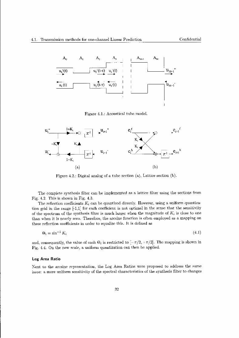
One way of representing the LP coefficients is by reflection coefficients (RC). This denomination is a result of the interpretation as physical parameters of an acoustical tube. In speech coding, where LP is a much applied tool, an acoustical tube is used to model the vocal tract. The model consists of a series of cylindrical tube sections with different diameters (see Fig 4.1), and can be described by reflection coefficients.
Reflection coefficients have the property that the associated filter is unconditionally stable if all the coefficients are of magnitude less than one. We note that the reflection coefficients are directly available, as intermediate variables, when the Levinson-Durbin algorithm (see appendix B) is used for solving the LP equations. In speech coding, acoustical tubes are used for modelling the vocal tract, and in the digital analog (see Fig. 4.2), the successive sections are specified by the reflection coefficients Ki.
31
4.1. Transmission methods for one-channel Linear Prediction Confidential
Ao Al Az A3 AM-1 AM
I UMH. u0+(t) u/(t-'t) u/(t) - - - ------ -----
..,._ ..,._ u0·(t) u2·(t-'t) u3·(t) I UM+l
-
I
Figure 4.1.: Acoustical tube model.
K, I ,------, u -_____..,..-~r--- i+l
1-K;
(a) (b)
Figure 4.2.: Digital analog of a tube section (a), Lattice section (b).
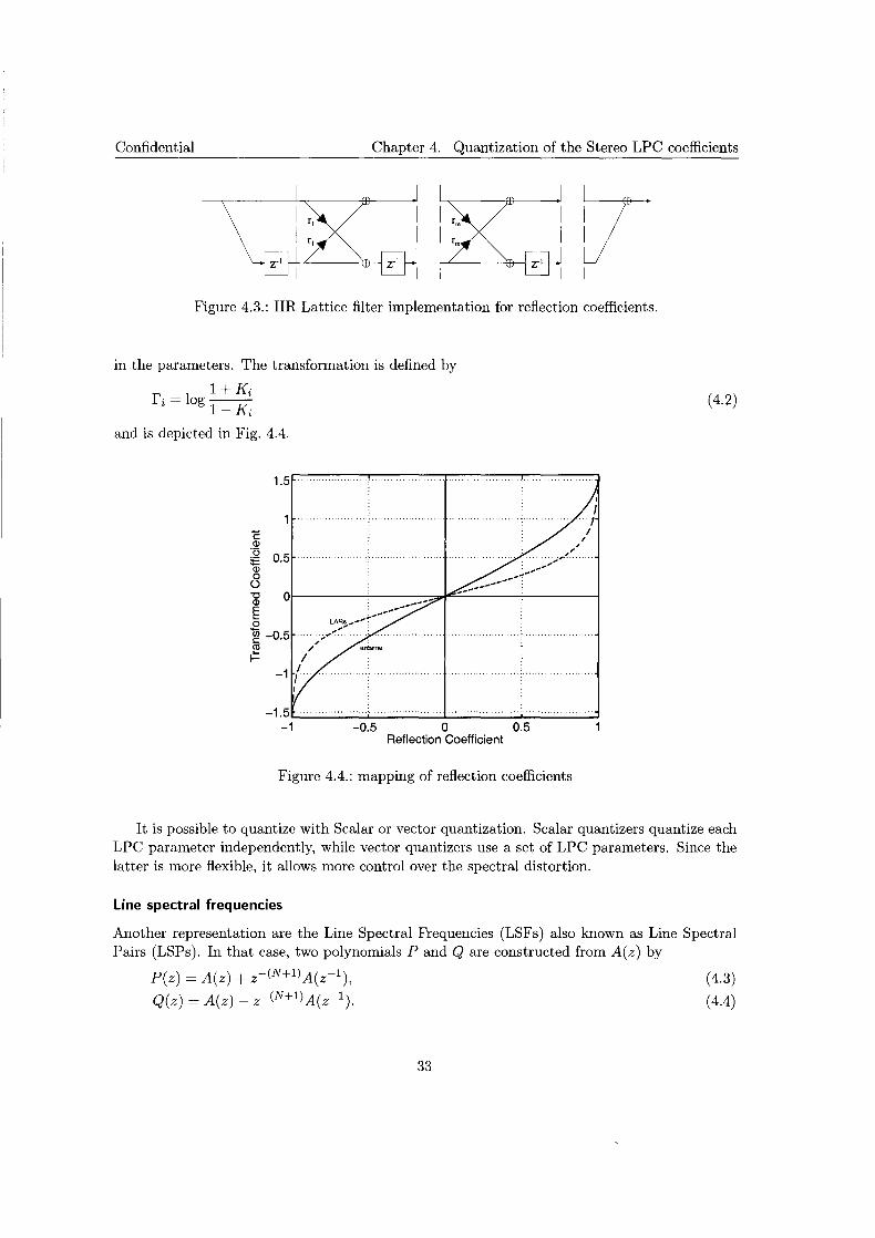
The complete synthesis filter can be implemented as a lattice filter using the sections from Fig. 4.2. This is shown in Fig. 4.3.
The reflection coefficients Ki can be quantized directly. However, using a uniform quantization grid in the range [-1,1] for each coefficient is not optimal in the sense that the sensitivity of the spectrum of the synthesis filter is much larger when the magnitude of Ki is close to one than when it is nearly zero. Therefore, the arcsine function is often employed as a mapping on these reflection coefficients in order to equalize this. It is defined as
( 4.1)
and, consequently, the value of each ei is restricted to [ -1r /2, +1r /2]. The mapping is shown in Fig. 4.4. On the new scale, a uniform quantization can then be applied.
Log Area Ratio
Next to the arcsine representation, the Log Area Ratios were proposed to address the same issue: a more uniform sensitivity of the spectral characteristics of the synthesis filter to changes
32
Confidential Chapter 4. Quantization of the Stereo LPC coefficients
Figure 4.3.: IIR Lattice filter implementation for reflection coefficients.
in the parameters. The transformation is defined by
ri =log 1 + Ki 1-Ki
and is depicted in Fig. 4.4.
-0.5 0 0.5 Reflection Coefficient
Figure 4.4.: mapping of reflection coefficients
(4.2)
It is possible to quantize with Scalar or vector quantization. Scalar quantizers quantize each LPC parameter independently, while vector quantizers use a set of LPC parameters. Since the latter is more flexible, it allows more control over the spectral distortion.
Line spectral frequencies
Another representation are the Line Spectral Frequencies (LSFs) also known as Line Spectral Pairs (LSPs). In that case, two polynomials P and Q are constructed from A(z) by
P(z) = A(z) + z-(N+1l A(z-1 ),
Q(z) = A(z)- z-(N+1) A(z-1 ).
33
(4.3)
( 4.4)
---------------------------------------------------------
4.2. Quantization of two-channel prediction parameters Confidential
If A(z) is minimum phase polynomial, then all the roots of P(z) and Q(z) lie on the unit circle. Furthermore, the roots of P(z) and Q(z) are interspersed. Thus, the LSFs are ordered and bounded. There is also a physical interpretation possible of these two polynomials [29]: P(z) corresponds to the vocal tract with the glottis closed and Q(z) with the glottis open.
4.2. Quantization of two-channel prediction parameters
For two-channel LP systems, the quantization of the filter coefficients is an unknown territory. The one-channel approaches described before do not apply immediately: they have to be adapted or extended in order to be applicable to the two-channel case. We describe two preliminary ideas on the quantization. We do not consider direct quantization of the matrix polynomial coefficients because, from the experience in the one-channel case, we assume that is about the worst you can do.
4.2.1. Reflection Matrices
Since the two-channel case is in so-far identical to the one-channel case that a (block-)Levinson algorithm applies, and since in the one-channel case both the arcsine and the LAR representation are coupled to the reflection coefficients, it seems worthwhile to consider the reflection matrices as arising in the block-Levinson algorithm as a possible source for quantization strategies.
A first problem that appears here is that, in contrast to the one-channel case, two sets of reflection matrices appear in a block-Levinson algorithm: one for the forward and one for the backward recursion. Having either one of them is insufficient to start the recursion. Therefore, transmission of the reflection matrices does not seem to be cost effective. Fortunately, both forward and backward reflection matrices can be derived from the so-called normalized reflection matrices. To do this, data concerning one additional matrix has to be transmitted. This data is then iteratively updated in order to be able to construct both reflection matrices from the normalized one.
A possible way for transmitting a (normalized) reflection matrix could be the following. As any matrix, it can be decomposed by either a singular value decomposition or an eigenvalue decomposition. In both cases, we obtain 2 rotation angles (coupled to the unitary matrices or the eigenvectors) and the singular values or eigenvalues. It is believed that transmitting these singular values or eigenvalues in the form of and arcsine or LAR presentation could be a possible way. Of course, it would also be possible to code both the eigenvalues in some (arithmetic/geometric) mean and difference value. Furthermore, the angles coupled to the vectors can be quantized as well, with an accuracy possibly dependent on the strength of its associated singular or eigenvalue.
4.2.2. Coupling to OCS parameters
In view of the experience and knowledge obtained with quantizing the Interaural Time Difference (lTD), Interaural Level Difference (ILD) and coherence values in OCS (subsection 2.2.6), it would be advantageous to have a coupling between these parameters and the parameters of a two-channel LP system. Although the description of the LP system in terms of an all-pass line
34

Confidential Chapter 4. Quantization of the Stereo LPC coefficients
(3.13) suggest that that is not impossible since the all-pass is a warping device and, consequently, DFT-transforms act like a uniform sampling on a perceptual frequency (Bark) scale (just like OCS), the relation between the OCS parameters and the two-channel LP parameters is certainly not straightforward. To start with, the LP system uses 4 parameters per section, where one could say that OCS works with 3 parameters per section. The extra fourth parameter in the LP system has probably to do with the overall whitening of both channels, an effect not taken into account in OCS.
So far, no research has been carried out on this specific topic. This is recommended because presumably this does not only lead to a method of quantization, but can also deepen our insights in both systems.
35

4.2. Quantization of two-channel prediction parameters Confidential
36

5. Signal quantization experiments
Next to the parameters (LP coefficients and rotation angle), other necessary information which needs to be transmitted or stored for reconstruction, are the rotated residual signals (main and side signal). If the proposed system is to compete with the state-of-the-art audio coders, it is also necessary to quantize these signals as efficiently as possible.
The bits spent on the parameters (or side information) are just assumed to be a small fraction of the total bit rate, because these parameters are transmitted only once per frame. The overall bit rate is therefore mainly determined by the costs of transmitting the residual signals. Therefore, several experiments were conducted to establish which parts or components of these main and side signals are essential in order to maintain a good quality of the reconstructed signal, and which parts can be compromised. These experiments (sections 5.2-5.7) were done with a collection of divers excerpts (see appendix A.3), representing different musical and speech(-like) signals.
Before discussing these experiments, we will first show the functioning of the system through an example (section 5.1).
Note that the experiments do not aim at removing psycho-acoustical irrelevancies, the purpose of the conducted experiments is examining how removing parts of the main and side signal affects the output. For removing the irrelevancies more insight into the proposed system and the inclusion of an appropriate psycho-acoustical model is needed.
5.1. Signals in the system
By means of plotting the different intermediate signals, we demonstrate the operation of the proposed analysis system. This is done for a part of an excerpt and with a sufficiently high prediction filter order, but similar results are achieved for other excerpts. Furthermore, we consider the estimated synthesis system.
Analysis system
The input signal, used for this example, is spread over multiple frames. It consists of both tonal and noise-like parts (Fig. 5.l(a)), and has an non-flat spectrum (Fig. 5.l(b)). Moreover, some similarities between both channels can be detected in the time domain.
The residual signals (e1 and ez), from which the predicted components have been removed, are shown in Fig. 5.2. The tonal parts of the input are almost completely removed (Fig. 5.2(a)), because of the high predictability of these parts. Furthermore, a clear drop in amplitude can be seen (cf. scales of y-axis in Fig. 5.l(a) and 5.2(a)), not only for the tonal parts but also for the
37

5.1. Signals in the system Confidential
more noise-like parts. This results in a drop of total energy and, in addition, energy is evenly distributed resulting in a nearly flat spectrum (Fig. 5.2(b)), because of redundancy removal.
Finally, possible correlation between sample pairs is removed through the rotator. This correlation at lag zero can still exists, because the LP only makes an estimates according to the history of both input signals, but not from the current samples. Therefore, after rotation we see a lower amplitude for the side signal, and a slight increase for the main signal (Fig. 5.3(a)). Furthermore, the spectrally flatter character is still maintained after rotation (Fig. 5.3(b) ).
INPUT
f[kHz] 22
t[ms] f[kHz]
(a) (b)
Figure 5.1.: Input signal in: Time domain (a), Frequency domain (b).
RESIDUAL RESIDUAL
.. ~~~ t[ms]
0 22
.. 1 ~~-~~· l:~~ <;!
-0 0:
0 0 22 t[ms] f[kHz]
(a) (b)
Figure 5.2.: Residual signals in: Time domain (a), Frequency domain (b).
Now, for the same example, an additional explanation is given according to Lissajous plots, in these plots the current sample of one channel is plotted against the current sample of the other channel for different instances in time. The Lissajous plot of the input (Fig. 5.4( a)) shows a strong dependence between both channels (here the mono component). Next, the residual signal, which results after LP, has a much lower variance than the input (Fig. 5.4(b)), but the dependence between the sample pairs of the channels still exists, with almost the same orientation as the input. Therefore, the rotator is used for removing this last correlation. The
38
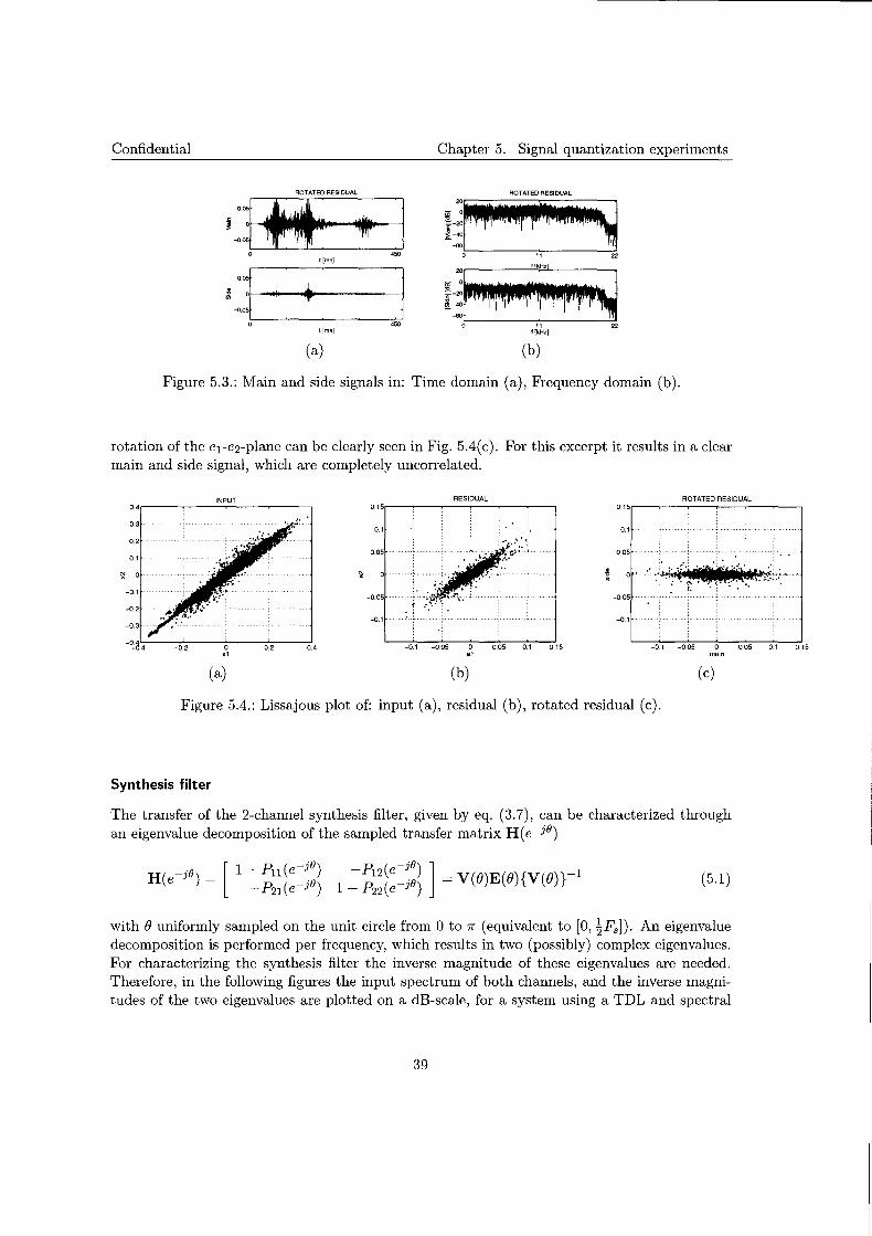
Confidential Chapter 5. Signal quantization experiments
ROTATED RESIDUAL
~~~~~~ 0 11 22
~~ 0 11 22
f{kHz]
450 t[ms]
0051 j -oo:f-----··+to------1
0~-~-----~-~.~~ t[ms]
(a) (b)
Figure 5.3.: Main and side signals in: Time domain (a), Frequency domain (b).
rotation of the e1-ez-plane can be clearly seen in Fig. 5.4(c). For this excerpt it results in a clear main and side signal, which are completely uncorrelated.
INPUT o.•,--~----'C..C..,.:.---'------,
(a)
RESIDUAL
-0.1 -0.05 0 e1
(b)
0 • ·: ... ~~~fl.,ll.t~~t~h:.:-0 :. • •••
-01
0.15
(c)
Figure 5.4.: Lissajous plot of: input (a), residual (b), rotated residual (c).
Synthesis filter
The transfer of the 2-channel synthesis filter, given by eq. (3.7), can be characterized through an eigenvalue decomposition of the sampled transfer matrix H( e-1 11 )
(5.1)
with() uniformly sampled on the unit circle from 0 to 7r (equivalent to [0, !F8 ]). An eigenvalue decomposition is performed per frequency, which results in two (possibly) complex eigenvalues. For characterizing the synthesis filter the inverse magnitude of these eigenvalues are needed. Therefore, in the following figures the input spectrum of both channels, and the inverse magnitudes of the two eigenvalues are plotted on a dB-scale, for a system using a TDL and spectral
39
0.15
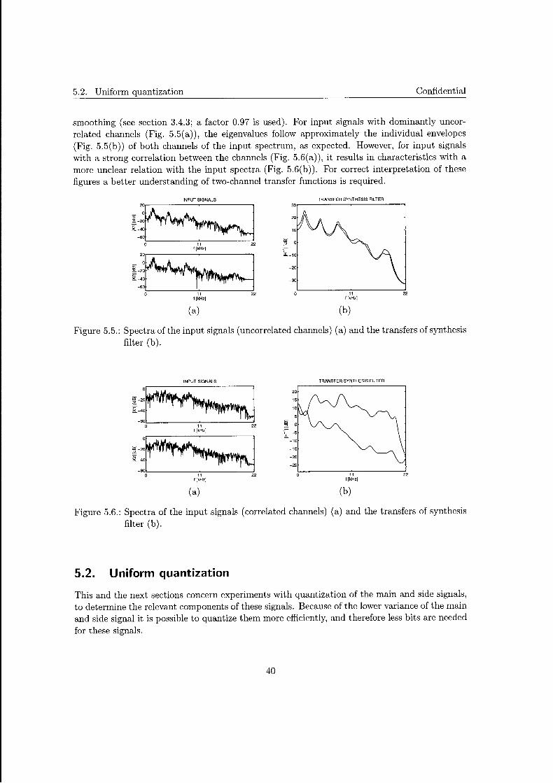
5.2. Uniform quantization Confidential
smoothing (see section 3.4.3; a factor 0.97 is used). For input signals with dominantly uncorrelated channels (Fig. 5.5(a)), the eigenvalues follow approximately the individual envelopes (Fig. 5.5(b)) of both channels of the input spectrum, as expected. However, for input signals with a strong correlation between the channels (Fig. 5.6(a)), it results in characteristics with a more unclear relation with the input spectra (Fig. 5.6(b)). For correct interpretation of these figures a better understanding of two-channel transfer functions is required.
INPUT SIGNALS
~-:~~-.AAho l ~-40~ r, ... ,,, ntr""l~
-BOO~-----:,":-, -------}22 l[kHz]
!-:~~ ~-40
-SOL__ ____ _:_._ ____ __.J
0 11 22 I[ kHz]
(a)
TRANSFER SYNTHESIS FILTER
(b)
Figure 5.5.: Spectra of the input signals ( uncorrelated channels) (a) and the transfers of synthesis filter (b).
INPUT SIGNALS
~·~ ~-40~ -WOL-----~,-,---~~22
l[kHz]
!-~~ ~-40
-00'------~----~ a 11 22 I[ kHz]
(a)
TRANSFER SYNTHESIS FJL TEA
(b)
Figure 5.6.: Spectra of the input signals (correlated channels) (a) and the transfers of synthesis filter (b).
5.2. Uniform quantization
This and the next sections concern experiments with quantization of the main and side signals, to determine the relevant components of these signals. Because of the lower variance of the main and side signal it is possible to quantize them more efficiently, and therefore less bits are needed for these signals.
40
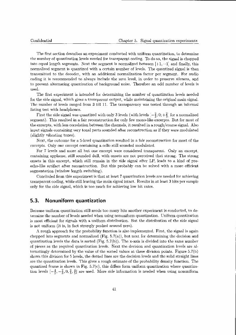
Confidential Chapter 5. Signal quantization experiments
The first section describes an experiment conducted with uniform quantization, to determine the number of quantization levels needed for transparent coding. To do so, the signal is chopped into equal length segments. Next the segment is normalized between [+1, -1] and finally, this normalized segment is quantized with a certain number of levels. The quantized signal is then transmitted to the decoder, with an additional normalization factor per segment. For audio coding it is recommended to always include the zero level, in order to preserve silences, and to prevent alternating quantization of background noise. Therefore an odd number of levels is used.
The first experiment is intended for determining the number of quantization levels needed for the side signal, which gives a transparent output, while maintaining the original main signal. The number of levels ranged from 3 till 11. The transparency was tested through an informal listing test with headphones.
First the side signal was quantized with only 3levels (with levels [-i; 0; +iJ for a normalized segment). This resulted in a fair reconstruction for only few mono-like excerpts. But for most of the excerpts, with less correlation between the channels, it resulted in a rough/coarse signal. Also input signals containing very tonal parts sounded after reconstruction as if they were modulated (slightly vibrating tones).
Next, the outcome for a 5-level quantization resulted in a fair reconstruction for most of the excerpts. Only one excerpt containing a cello still sounded modulated.
For 7 levels and more all but one excerpt were considered transparent. Only an excerpt, containing applause, still sounded dull, with onsets are not perceived that strong. The strong onsets in this excerpt, which still remain in the side signal after LP, leads to a kind of preecho-like artifact after reconstruction. But this probably can be solved with a more efficient segmentation (window length switching).
Concluded from this experiment is that at least 7 quantization levels are needed for achieving transparent coding, while still leaving the main signal intact. Results in at least 3 bits per sample only for the side signal, which is too much for achieving low bit rates.
5.3. Nonuniform quantization
Because uniform quantization still needs too many bits another experiment is conducted, to determine the number of levels needed when using nonuniform quantization. Uniform quantization is most efficient for signals with a uniform distribution. But the distribution of the side signal is not uniform (it is, in fact strongly peaked around zero).
A rough approach for the probability function is also implemented. First, the signal is again chopped into segments and normalized (Fig. 5.7(a)), but next for determining the decision and quantization levels the data is sorted (Fig. 5. 7(b) ). The x-axis is divided into the same number of pieces as the required quantization levels. Next the decision and quantization levels are alternatingly determined by the value of the sorted values at these division points. Figure 5. 7(b) shows this division for 5 levels, the dotted lines are the decision levels and the solid straight lines are the quantization levels. This gives a rough estimate of the probability density function. The quantized frame is shown in Fig. 5.7(c), this differs form uniform quantization where quantization levels [-i, -~, 0, ~' tl are used. More side information is needed when using nonuniform
41
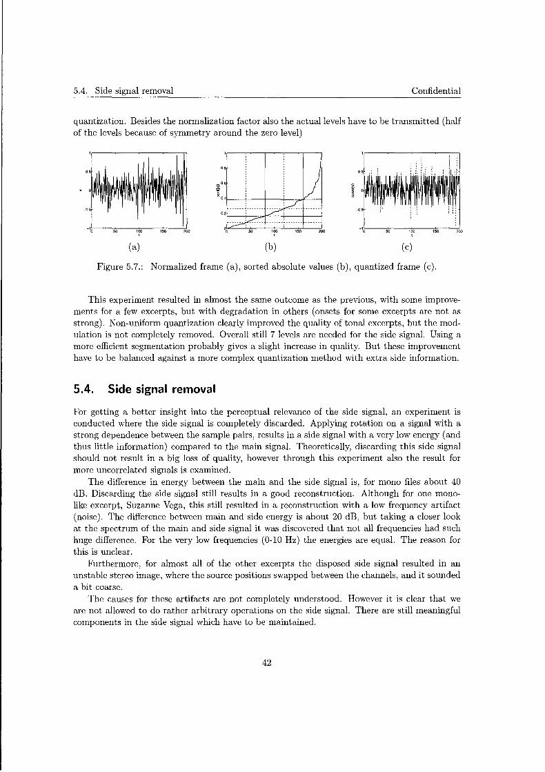
5.4. Side signal removal Confidential
quantization. Besides the normalization factor also the actual levels have to be transmitted (half of the levels because of symmetry around the zero level)
-1o!:------:so-o ----,1ooc:---~1so:::---'=!2oo 1
(a)
0.8
:::::::0.6
~ ~ 0 'f---'------ll--'----..,..fL___-l
(b)
- 1o'----...,soo-----~1oo,..--""'1s::-o --':,'200 1
(c)
Figure 5.7.: Normalized frame (a), sorted absolute values (b), quantized frame (c).
This experiment resulted in almost the same outcome as the previous, with some improvements for a few excerpts, but with degradation in others (onsets for some excerpts are not as strong). Non-uniform quantization clearly improved the quality of tonal excerpts, but the modulation is not completely removed. Overall still 7 levels are needed for the side signal. Using a more efficient segmentation probably gives a slight increase in quality. But these improvement have to be balanced against a more complex quantization method with extra side information.
5.4. Side signal removal
For getting a better insight into the perceptual relevance of the side signal, an experiment is conducted where the side signal is completely discarded. Applying rotation on a signal with a strong dependence between the sample pairs, results in a side signal with a very low energy (and thus little information) compared to the main signal. Theoretically, discarding this side signal should not result in a big loss of quality, however through this experiment also the result for more uncorrelated signals is examined.
The difference in energy between the main and the side signal is, for mono files about 40 dB. Discarding the side signal still results in a good reconstruction. Although for one monolike excerpt, Suzanne Vega, this still resulted in a reconstruction with a low frequency artifact (noise). The difference between main and side energy is about 20 dB, but taking a closer look at the spectrum of the main and side signal it was discovered that not all frequencies had such huge difference. For the very low frequencies (0-10 Hz) the energies are equal. The reason for this is unclear.
Furthermore, for almost all of the other excerpts the disposed side signal resulted in an unstable stereo image, where the source positions swapped between the channels, and it sounded a bit coarse.
The causes for these artifacts are not completely understood. However it is clear that we are not allowed to do rather arbitrary operations on the side signal. There are still meaningful components in the side signal which have to be maintained.
42

Confidential Chapter 5. Signal quantization experiments
5.5. Synthetic side signal
As described in the outcome of the previous experiment, the side signal still contains information on the position of the source, and this can not be discarded. Therefore, another experiment is conducted were a synthetic side signal is generated at de decoder side, to compensate for the loss in energy resulting after discarding the side signal.
Generating the synthetic side signal is done similar to OCS and VECMA. It is made by delaying the main signal (about 500 samples), to decorrelated it with the main signal (originally main and side signals are orthogonal) (Fig. 5.8). Next, the total energy of the frame is corrected, according to a scale factor determined at the encoder, for which one extra parameter is needed.
Again an informal listening test was used for determining the quality of this method. The synthetic side signal resolved the unstable stereo image issue. The source positions are now maintained, but it sounded very noisy, i.e. low frequency noise (below 250 Hz), for all the non-mono excerpts.
IR X LP-s
Figure 5.8.: Create Side out of delayed main signal.
5.6. Partial side signal transmission
Considering the previous two experiments, which both have low frequency artifacts, a follow up experiment is tried. Now only the low frequency (3-4kHz) part of the side signal (LF-side) is transmitted, omitting everything else. This resulted in a stable stereo image but still a somewhat noisy reconstruction. But the main problem, i.e. an unstable stereo image, which occurred when removing the side signal completely, were absent. Furthermore, the reconstruction is less noisy than with a synthetic side signal. This implies that most of the meaningful information of the side signal is in the low frequency part.
Next, this low frequency side signal is combined with the 'missing' high frequency part of the synthetic side signal. This resulted in an overall improvement, and led to fair results where most of the noise was removed.
The conclusion from these experiments is that a reduction to one channel is not directly possible, but fair result can been achieved with the original LF-side signal combined with the synthetic signal, which is an equivalent to a 1.1-channel system (in bandwidth) instead of a 2-channel.
43

5.7. Spectral bandwidth replication Confidential
5. 7. Spectral bandwidth replication
As done in speech coding, and more recently also applied in audio coding [11], we applied Spectral Bandwidth Replication (SBR) for reducing the total bandwidth.
With SBR (used in HE-AAC and MP3Pro) only the lower frequency part, i.e. half of the bandwidth, is transmitted, because of the lower psycho-acoustical importance of the temporal signal structure at high frequencies. In the decoder the reconstruction of the high frequency part is done by mapping the low frequency part to the missing high frequencies. Then these are shaped through some scaling data, in order to match the original data and finally some tonal and noise-like parts can be added. This bandwidth reduction makes it a very useful tool for applications which require low bit rate audio coding.
A sufficiently high prediction order used in the proposed scheme, results in a residual signal with a spectrally flat envelope, and which is still maintained after rotation (Fig. 5. 9( a)). Because of this signal property it is much easier to apply SBR, making it less complex. The main and/or side signal is downsampled with a decimation factor of 2 and 3th order Chebyshev filter, saving half the bandwidth. At the decoder the signals are upsampled again, resulting in a mirrored version of the lower part at the higher frequencies (Fig. 5.9(b)). No additional side information is needed because of the spectrally flat nature of the main and side signal. There is only a small aliaising difference at the highest frequencies, but this will be shaped through the synthesis filter.
ROTATED RESIDUALS
~-:~-.:J E-40
r1. I II"., .. ,I. ·.~' '11'1 '1 ··~
-B~.L------:,:':-,----~22 f [kHz]
20~ CD o ~ -20 til -40
-S~L------,:';-,----~22 f [kHz]
(a)
ROTATED RESIDUALS
~-:~-E _40
r I . I I'" I' I • 'I I 1· . ·1 I I' 'I 'I "I I I . I ]
-B~.L------:,,....-------=!.22 f[kHz]
20~ CD o ~ -20 Cl) -40
-B~.L-------:,,...-------=!.22 f[kHz]
(b)
Figure 5.9.: Original main and side signals (a), main and side signal after mirroring at de decoder side.
Two experiments where conducted, first applying SBR on the side signal only, and next applying SBR on both side and main signal, generated using prediction order 20.
Only SBR on the side signal results in almost transparent reconstructions for most of the excerpts. Only a small difference was perceived for the castanets excerpt, in which some high frequency noise can be heard. Applying SBR on both main and side resulted a slight degradation for some of the excerpts (compared to the previous experiment), e.g. in the castanets more high frequency noise is introduced.
Main conclusion is that the quality is good, although not completely transparent for all excerpts.
44
Confidential Chapter 5. Signal quantization experiments
5.8. Conclusion from the experiments
From the experiments we conclude that the side signal can not be discarded completely. There are still meaningful components in the side signal which have to be maintained, but other experiments indicate that most important components are within the lower frequency region.
The most promising technique for attaining a low bit rate is bandwidth reduction through SBR, which can be easily used on the spectrally flat signals. Furthermore, it can be applied on the side signal as well as on the main signal, resulting in the equivalent bandwidth of one mono channel. Overall, we can probably do slightly better than OCS/BCC, because the side signal can be reduced even further, and this suggests that low bit rate coders based on the proposed system are feasible.
45

5.8. Conclusion from the experiments Confidential
46

6. Conclusions and Recommendations
6.1. Conclusions
The aim of this thesis was to explore a stereo coding technique capable of providing similar or better performance, in quality /bit rate balance, than existing coders, and for both the high and the low bit rate levels. It was argued that known stereo coding techniques do not simultaneously deliver the best performance at both bit rate levels.
Considered was a 2-channel Linear Prediction (LP) plus rotator, since this allows perfect reconstruction (which is in line with the best quality at high bit rate end) and allows the construction of a main and side signal (similar to OCS; the best low bit rate stereo coding tool).
For the proposed system it was shown that the optimization dissolves in two separate stages: optimizing the stereo LP and subsequently optimizing the rotator with the residual from the Stereo LP. For the prediction filters Laguerre filters are chosen, because of their close resemblance with the psycho-acoustical Bark-scale, which is advantageous for lossy audio coding. For equal cross and auto prediction orders the block Levinson algorithm applies, which is an efficient way of optimizing the Stereo LP. The block Levinson algorithm implies that the synthesis system is stable, for equal orders, and that the required order can be adaptively determined.
This system is implemented and tested. The tests show that the implemented system operates as expected. Special care was needed for some pathological input signals.
A number of informal listening experiments were performed to establish which components of the residual signal have to be maintained in a transmission system and which parts can be compromised. Discarding the side signal completely gives problems for most cases, but fair results are already achieved by only transmitting 10% of the side signal (only low frequencies). But in view of the spectral flattening, Spectral Band Replication (SBR) appears to be a method which allows low bit rate coding for the proposed system.
47

6.2. Recommendations Confidential
6.2. Recommendations
On basis of the research reported here and in line with the conclusions given above, we have the following list of recommendations:
• Regularization needs to be considered in more detail, this thesis only describes preliminarily solutions.
• Efficient quantization techniques for the parameters have to be developed, two possible directions for this are suggested within this thesis.
• To get a better insight into the required bit rate for the transmission of the residual signal, more experiments are required. This in order to pin down the essential components of the residual signal.
• Finally, the total complexity has to be estimated and compared with the existing coding systems.
48
A. Lists of abbreviations, notations and used excerpts
A.l. List of abbreviations
BCC CELP DFT FFT FIR HE-AAC ICLD ICTD IID IIR ILD lTD LAR LP LPC LSF LSP LWR ocs PCA PCM SBR SVD TDL VECMA
Binaural Cue Coding Code Excited Linear Prediction Discrete Fourier Transform Fast Fourier Transform Finite Impulse Response High Efficiency Advanced Audio Coding Inter Channel Level Differences Inter Channel Time Differences Interaural Intensity Differences Infinite Impulse Response Interaural Level Differences Interaural Time Differences Log Area Ratios Linear Prediction Linear Predictive Coding Line Spectral Frequencies Line Spectral Pairs Levinson Wiggins Robinson algorithm Optimum Coding of Stereo Principle Component Analysis Pulse Code Modulation Spectral Bandwidth Replication Singular Value Decomposition Tapped Delay Line Very Efficient Coding of Multichannel Audio
49

A.2. List of notations
A.2. List of notations
Symbol Explanation a, b, c A,B,D x[n] X(z) x x A,B,C Q,Q,f X!
X2 A(m)
Operator
* c*
Lowercase letters are signals in the time domain Uppercase letters are signals in the frequency domain Discrete time index n of signal x Frequency index z of signal X Predicted signal of x Reconstructed signal of x Bold uppercase letters are matrices Underlined lowercase letters are vectors Left channel of stereo signal Right channel of stereo signal Matrix A in a loop at iteration m
Explanation convolution Complex conjugated of c Determinant of matrix A Inverse of matrix A Transpose of matrix A Complex conjugate of matrix A Conjugate transpose of matrix A
A.3. List of used excerpts
The following excerpts are used all wav-files with a sample frequency of 44 1 kHz. '
Title Content Duration Suzanne Vega- Tom's Diner Voice (mono-like) 0:10 German male Voice (mono-like) 0:08 Speech English Female Voice (mono-like) 0:07 Trumpet Single instrument 0:10 Orchestra Multiple instruments 0:12 Quiz Tune Multiple instruments 0:11 Harpsichords Single instrument 0:07 Castanets Single instrument 0:07 Harmonica Single instrument 0:27 Bag pipes Single instrument 0:11 Xylophone Single instrument 0:10 Piano Single instrument 0:13 Applause Applause 0:10 Pop Multiple instruments 0:10 Byrds - Eight Miles High Multiple instruments 0:33 Carmen- L'amour est un oiseau rebelle Opera 0:10
50
Confidential
B. One-channel linear prediction
For removing redundancies within an (audio) signal, Linear Prediction (LP) [35, 28] can be used. This because successive samples are often highly correlated. So it should be possible to get a good estimate of the current sample from its preceding ones and thereby to decorrelate the samples. The predicted signal is modelled as a linear combination of its past values by
N
x[nJ = :L akx[n- kJ (B.l) k=l
with the prediction signal x, the weights ak as linear predictor coefficients and N is the number of preceding samples being used in the prediction (prediction order). The error which remains after subtracting the predicted signal x[n] from the original x[n] is called the prediction residual or prediction error e[n] and is given by
N
e[nJ = x[nJ- x[nJ = x[nJ- :L akx[n- kJ. k=l
(B.2)
Such a system is called an one-step ahead predictor because it tries to predict the next sample from its previous ones. This results in an all-zero prediction filter, of order N (see Fig. B.l), and with an impulse response a[k] = -ak (k = l..N with a[O] = 1). The corresponding transfer function of the analysis filter is given by
N
A(z) = Lakz-k (B.3) k=O
With the correct predictor coefficients (the computation of these optimal parameters will be explained later on), the short-term correlations between samples of the residual have been minimized, and this leads to an approximately flat spectral envelope for the residual, that is if a sufficiently high order is used. Therefore, the analysis filter is also known as a whitening filter.
The variance of the residual is lower (or equal for a signal with no correlation) than the original, therefore it can be quantized more efficiently. However, this is signal dependent, because some signals are more predictable than others. This ratio in variances of the residual and the input signal is called the prediction gain, and is defined as
or (B.4)
51
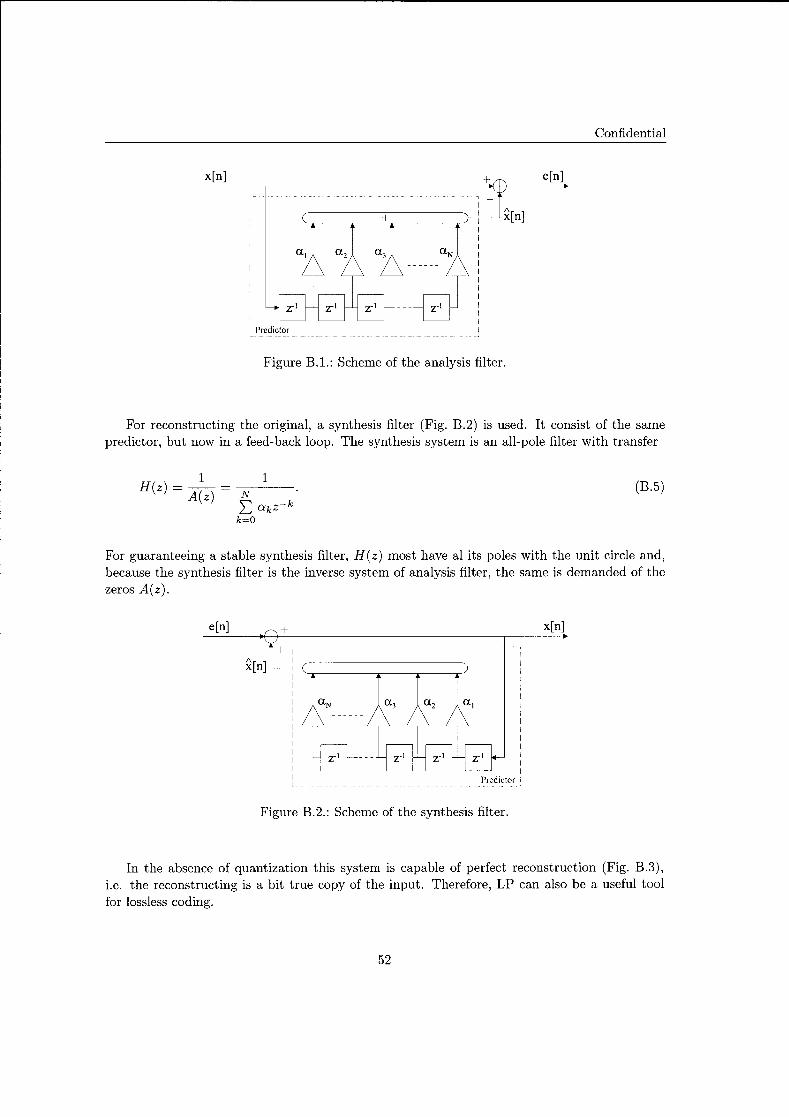
Confidential
~[n]
Predictor
Figure B.l.: Scheme of the analysis filter.
For reconstructing the original, a synthesis filter (Fig. B.2) is used. It consist of the same predictor, but now in a feed-back loop. The synthesis system is an all-pole filter with transfer
(B.5)
For guaranteeing a stable synthesis filter, H(z) most have al its poles with the unit circle and, because the synthesis filter is the inverse system of analysis filter, the same is demanded of the zeros A(z).
e[n] x[n]
Predictor
Figure B.2.: Scheme of the synthesis filter.
In the absence of quantization this system is capable of perfect reconstruction (Fig. B.3), i.e. the reconstructing is a bit true copy of the input. Therefore, LP can also be a useful tool for lossless coding.
52
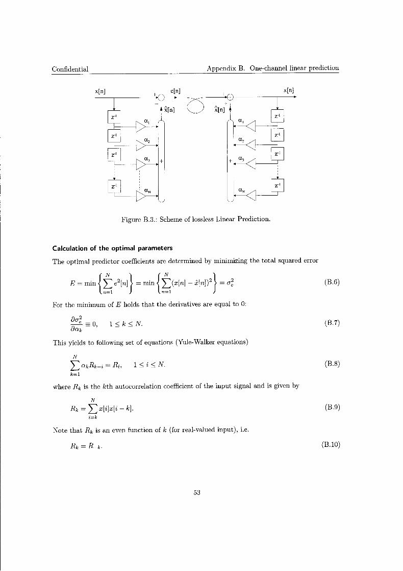
Confidential Appendix B. One-channel linear prediction
x[n] + e[n] x[n]
Figure B.3.: Scheme of lossless Linear Prediction.
Calculation of the optimal parameters
The optimal predictor coefficients are determined by minimizing the total squared error
E ~min {t, e2[n]} ~min {t,(x[n[- X[n])2} ~a;
For the minimum of E holds that the derivatives are equal to 0:
1 :::; k :::; N.
This yields to following set of equations (Yule-Walker equations)
N
L DkRk-i = Ri,
k=l
1 :::; i :::; N.
where Rk is the kth autocorrelation coefficient of the input signal and is given by
N
Rk = L_x[i]x[i- k]. i=k
Note that Rk is an even function of k (for real-valued input), i.e.
53
(B.6)
(B.7)
(B.8)
(B.9)
(B.10)
Confidential
Equation B.8 can be rewritten in a matrix notation
Rg=r. (B.ll)
with the (N x N) autocorrelation matrix R given by
Ro R-1 R_z R-N+l R1 Ro R-1 R-N+2
R= Rz R1 Ro R-N-3 (B.12)
RN-1 RN-2 RN-3 Ro
which has a Hermitian Toeplitz structure and in the case of real-valued input signals a symmetric Toeplitz structure. The optimal prediction coefficients are stacked into a vector (g = [a1,a2,··· ,aN]t),andr.isalsoastackedvector(g= [R1,Rz,··· ,RN]t). Theoptimalprediction coefficients can be computed by solving B.ll, this results in
(B.13)
Using the autocorrelation method this requires ~3 + O(N2) operations (multiplications and
divisions) [35]. However, by making use of the structure of the matrix R (symmetric Toeplitz) it is possible
to solve B.13 in a more efficient manner. Like in the recursive Levinson-Durbin algorithm which also makes use of the fact that the vector r. comprises the same elements as in the autocorrelation matrix R. The algorithm can be specified as follows
Eo Ro (B.14a)
R + LN i-lR
ki i k=1 aj i-j
(B.14b) Ei-1
( i) ai ki (B.l4c)
( i) aj
(i-1) + k (i-1) aj iai-j 1::;j:=;i-1 (B.14d)
Ei (1- kr)Ei-1 (B.14e)
Equations B.14 b-e are solved recursively for i = 1, 2, · · · , N, where (i) denotes the iteration step, and the intermediate ki are also known as reflection coefficients. This method requires only N 2 + O((N)) operations and, because also all solutions are computed for all orders less than N, it also possible to adaptively determine the order, by incorporating other stop conditions, e.g. dependent on the energy Ei.
54
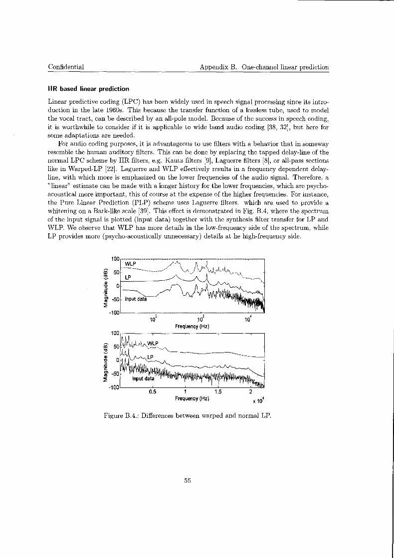
Confidential Appendix B. One-channel linear prediction
IIR based linear prediction
Linear predictive coding (LPC) has been widely used in speech signal processing since its introduction in the late 1960s. This because the transfer function of a lossless tube, used to model the vocal tract, can be described by an all-pole model. Because of the success in speech coding, it is worthwhile to consider if it is applicable to wide band audio coding [38, 32], but here for some adaptations are needed.
For audio coding purposes, it is advantageous to use filters with a behavior that in someway resemble the human auditory filters. This can be done by replacing the tapped delay-line of the normal LPC scheme by IIR filters, e.g. Kautz filters [9], Laguerre filters [8], or all-pass sections like in Warped-LP [22]. Laguerre and WLP effectively results in a frequency dependent delayline, with which more is emphasized on the lower frequencies of the audio signal. Therefore, a "linear" estimate can be made with a longer history for the lower frequencies, which are psychoacoustical more important, this of course at the expense of the higher frequencies. For instance, the Pure Linear Prediction (PLP) scheme uses Laguerre filters. which are used to provide a whitening on a Bark-like scale [39]. This effect is demonstrated in Fig. B.4, where the spectrum of the input signal is plotted (input data) together with the synthesis filter transfer for LP and WLP. We observe that WLP has more details in the low-frequency side of the spectrum, while LP provides more (psycho-acoustically unnecessary) details at he high-frequency side.
100 WLP /V'~. '\ •
10 ~-...._______ / \ 1-J~'..I\ j,,J
50 - A. j \., vJ; ~ V\ "0 LP ,, --A , --~\-----~ ._, G)
0 ~~ '0 .a ·c; ~ 01 -50 Ill ::.;!
-100 10
2 1d
4 10
Frequency (Hz)
ro ~ G) "0 :I
~ 01 Ill :2
-100 0.5 2
Frequency (Hz) X 10
4
Figure B.4.: Differences between warped and normal LP.
55

Confidential
56

C. Rotation
A basic building block in the proposed system is the rotator. Rotation, main axis transform, applying Singular Value Decomposition (SVD) or Principle Component Analysis (PCA) are all identical transformations, all with the same intention namely to minimize the covariance between sets of data.
Rotating over an angle cp (counter clockwise around the origin) in a two-dimensional plane is defined by multiplying the data sets with the transformation matrix R
R( ) = ( cos(cp) - sin(cp) ) . 'P sin( cp) cos( cp)
(C.l)
Note that the inverse rotation is equal to the rotation with the negative angle
(C.2)
For audio coding, rotation is used for removing correlations between the current samples of the two channels (Fig. C.l), which results in a main and a side signal.
e I m am
R
e 2 si de
_________ _. cp
Figure C.l.: Scheme of a 2-channel rotator.
Applying the matrix operation (eq. C.l) to the stereo signal (e1 and e2) results in the following
relation
( m[n] ) = ( cos(cp) - sin(cp) ) . ( e1[n] ) = ( el[n]· cos(cp)- e2[n]· sin(cp) ) (C 3) s[n] sin(cp) cos(cp) e2[n] el[n]· sin(cp) + e2[n]· cos(cp) · ·
For the mono-like input signal, shown in figure C.2(a), the strong dependence between channels can be easily detected in a Lissajous plot (in here current values of x1 are plotted against current values of x2 for different instances in time) (Fig. C.3(a)). After rotation it results in a main signal (m[n]) with the mono component, and a low energy side signal with the "differences" of both channels (C.2(b)). The second Lissajous plot (Fig. C.3(b)) shows clearly the rotation of the x1 - x2-plane, and also the orthogonality (uncorrelated) of the main and side signal.
57
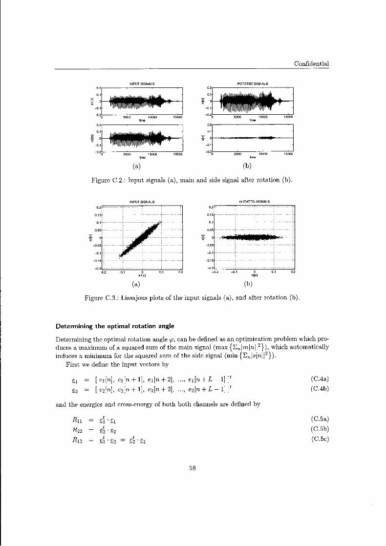
INPUT SIGNALS ROTATED SIGNALS
~ ::1~---------' -0.1-
-0.20L_ __ -:::':": __ ---,.:-~--.,.,.....,_,.J
"'" . : I 5000 10000 15000
time time
(a) (b)
Figure C.2.: Input signals (a), main and side signal after rotation (b).
INPUT SIGNALS
~··· -o~o~2:'-'-"-"--""'o.""1 =="'--~o ====""'o.1====~o.2
e1[n[
(a)
ROTATED SIGNALS
(b)
Confidential
Figure C.3.: Lissajous plots of the input signals (a), and after rotation (b).
Determining the optimal rotation angle
Determining the optimal rotation angle cp, can be defined as an optimization problem which produces a maximum of a squared sum of the main signal (max {I;nlm[n]l2} ), which automatically induces a minimum for the squared sum of the side signal (min {I;nls[n]i2} ).
First we define the input vectors by
[ el[n], el[n + 1], e1[n + 2], ... , e1[n + L- 1]]t [ e2[n], e2[n + 1], e2[n + 2], ... , e2[n + L- 1]]t
and the energies and cross-energy of both both channels are defined by
Rn t ~1. ~1
R22 t ~2. ~2
R12 t ~1. ~2
t ~2. ~1
58
(C.4a)
(C.4b)
(C.5a)
(C.5b)
(C.5c)
Confidential Appendix C. Rotation
From the definition
(C.6)
with (C.4) and (C.5), J can be rewritten to:
Ru + Rzz Ru- Rzz . 1= 2
+ 2
cos(2<p)+Rlzsm(2<p). (C.7)
Since J is a periodic function with periodicity n, we infer the following: 1. the maximum of J is attained for values cp + kn ( k E N); 2. the minimum of J is attained for values (/; + kn (k E N); 3. the minimums and maximums are 1r /2 apart: (/; = cp + kn /2.
In particular, we have 1. Jo = ~(Ru + Rzz) is the mean value over all <p;
2. J1 = ~(Ru + Rzz) + J(Ru- Rzz)2 /4 + Rr2 the maximum of J;
3. ]z = ~(Ru + Rzz)- J(Ru - Rzz) 2 /4 + Rr2 the minimum of J. We note that there is always a maximum and minimum except when J(R11 - R 22 ) 2 /4 + Rr2 = 0. We define the modulation depth d as the ratio of the mean J0 and
the excursion from the mean:
d = 2 J(Ru- Rzz) 2 /4 + Rr2 ,
Ru + Rzz (C.8)
and 0 < d < 1. If d ~ 0, then action has to be taken to guarantee a well-defined solution.
Define
c = R u - Rzz + 1. R
2 1,2
and
¢ = L.c
We then have
J = Io +lei cos(2<p- ¢)
and thus
¢/2 (+kn),
cp + 1f /2 ( +kn).
To remove ambiguity, we take (/; = cp + 1r /2.
59
(C.9)
(C.lO)
(C.ll)
(C.12a)
(C.l2b)

Confidential
60
D. Relation between Laguerre and tapped-delay-line LP systems
In this appendix, it is shown that a two-channel LP Laguerre system is theoreticaly equivalent to a LP TDL system with prefiltering. The consequence of this equivalence is the following. Assume that for all input signals and under certain optimization conditions, the LP TDL system yields stable synthesis filters. Then, under the same optimization conditions, the optimized LP Laguerre system will do so as well.
The equivalence can be shown as follows. Consider the predictor transfers
-1 N ~ (->.+z-1)k-1 Pij(z) = z L:C:l:ij,k 1- >.z-1 1- >.z-1
k=1 (D.l)
We can rewrite this to
Pi ·(z) = z-1 L~=1 Dij,k~ ( ->. + z-1)k-1 (1- >.z-1)N-k - z-1Qij(z) J (1- >.z-1 )N (1 - >.z-1 )N
(D.2)
where Qij is a N- 1st order polynomial. In view of the N free coefficients Dij,k, the polynomial Qij is an arbitrary polynomial of order N- 1.
Consider now the transfers Hij. • Fori# j we have Hij = -Pij and, therefore, free parameters in the Laguerre cross-predictors is equivalent to free parameters in a TDL cross-predictor when operating on a filtered input signal where the pre-filter is given by the transfer function ( 1 - >.z-1 rN. • Fori= j we have Hii = 1- Pii· Bringing this under a common denominator yields
(D.3)
The polynomial Qij(z) is an Nth order polynomial with its constant term equal to one and all other coefficients are free. Also this is consistent with a pre-filtered TDL case.
In conclusion, the optimal Laguerre LP is identical to having a pre-filter running on both channels and performing a TDL-based LP. The latter procedure is however ill-conditioned for typical input signals.
From the previous analysis, the attained increased modelling capability at the low-frequency side of the spectrum for the Laguerre LP system with >. > 0 can be easily understood. The pre-filtering puts more emphasis on the LF part of the spectrum and, therefore, increased coding gain can be achieved when modelling that part accurately.
61

Confidential
62

E. Separability of optimization
Suppose we have two signal x1 and x2. Furthermore, we have a set of regressor signals Yk, k = 1, 2, · · · , 2K. Typically these will be filtered versions of Xt, e.g.,
Y2i-1
Y2i
(E.1)
(E.2)
where x1 and x2 are both filtered with the same set of filters hi, i = 1, 2, · · · , K. We construct the signal 11 according to
2K
11 = cos(¢)x1 + sin(¢)x2- L '"YkYk· k=l
Consider the criterion J with
n
We will see later on that there is typically a single maximum and a single minimum of J as a function of the free parameters ¢ and '"Y such that when minimising/maximising J we have in fact constructed a two-port (x1, x2) --> (m, s) with m and s the main and side signal.
Consider the maximum and minimum of J. These are called J1 and h and the associated
signals are /11 and 112:
and
J 1 max.p,'YJ,
J2 = max.p,'YJ,
{¢,1'} = argmax.p,'YJ,
{~,i'} = argmax.p,'YJ.
The coefficients '"Yk for which J attains its minimum or maximum are given by
Q'"Y = P = cos(¢)P(l) + sin(¢)P(2)
where
Qk,l LYt(n)yk(n), n
p(l) k Lxl(n)yk(n),
n
p(2) k L x2(n)yk(n).
n
63
(E.3)
(E.4)
(E.5)
(E.6)
(E.7)
(E.8)
(E.9)

Accordingly, we define
Q-1 p(l)'
Q-1p(2l,
cos(¢)1'(1) + sin(¢)'y(2l.
Confidential
(E.lO)
(E.ll)
(E.l2)
Thus, given an¢, the optimal coefficients 1 are known. Note that 1(1) and 1(2) can be determined independently from ¢. We further note that 1(1) and 1(2) can be interpreted as the solutions of the following minimization problems:
n
and
n
respectively, with
2K "' (1) e1 x1-~ lk Yk,
k=1
2K
e2 = X2- 2:: rk2)Yk·
k=1
(E.13)
(E.l4)
Consequently, both solutions can be considered to stem from the minimization of T1 + T2. We note that it is also possible to interpret these coefficients as solutions to the minimization of
n
This can be easily shown as follows. First note that minimization of To is equal to minimization of T(f. Setting the derivative of T(f equal to zero yields
(E.15)
(E.16)
where Y is a matrix containing the signals Yk: Y = [Y1, Y2, · · · , Y2K ]. Under the assumption that ei e2 ::/:- 0 (this is only attainable in pathological cases), this leads to
(-Yt)(x2- Y1(2))
(-Yt)(x1- yl(ll)
0,
0,
i.e, equivalent conditions to (E.lO) and (E.ll).
64
(E.17)
(E.18)
Confidential Appendix E. Separability of optimization
Consider now the optimal rjJ. We assume real-valued signals. We have
J = (cos(rjy)xi + sin(rjJ)x~ + /'tyt) · (cos(rjJ)x1 + sin(rjJ)x2 + Y')').
Eliminating /' using
/'=cos( rP )Q-1 p(l) +sin( rP )Q-1 p(2)
leads to
with
xixl- p(l)tQ-lp(ll,
X~X2- p(2)t Q-1 p(2)'
xi X2 - p(l)t Q-1 p(2).
(E.19)
(E.20)
(E.21)
From Ru, R22 and R12, the optimal rjJ readily follows (for the maximum and the minimum of
J; see later). We can introduce the auxiliary signals
el = Xl- y/'(ll,
e2 = x2 - Y ')'(2),
and have
t e1 e1, t e2e2, t el e2.
(E.22)
(E.23)
(E.24)
(E.25)
(E.26)
Thus, the problem of finding the optimal rjJ and /'k minimising/maximising J and of constructing e can be easily done in four steps: 1. finding the optimal /'(1) and 1'(2), 2. constructing the signals e1 and e2, 3. finding the optimal rotation (PCA) for the signals e1 and e2, 4. applying this rotator to these signals in order to construct the signals f-11 and f-12 corresponding to a maximum and minimum of J.
In conclusion, the original problem is now split into two separate stages, each involving a separate optimization. In the first two-channel system, we minimize the powers of e1 and e2 and absolute value of their cross-power. This results in spectrally flat signals e1 and e2 and a spectrally flat cross-power (under certain conditions for the filters hi)· In the second step, the rotator, we rotate the signals e1 and e1 such that the resulting signals are orthogonal.
65

Confidential
66
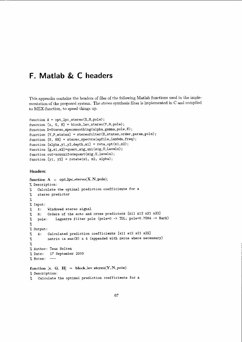
F. Matlab & C headers
This appendix contains the headers of files of the following Matlab functions used in the implementation of the proposed system. The stereo synthesis filter is implemented in C and compiled to MEX-function, to speed things up.
function A= opt_lpc_stereo(X,N,pole); function [x, G, H] = block_lev_stereo(Y,N,pole); function D=Stereo_specsmoothing(alpha,gamma,pole,N); function [Y,P,states] = stereofilter(X,states,order,param,pole); function [S, HH] = stereo_spectra(apfile,lambda,freq); function [alpha,y1,y2,depth,a1] = rota_opt(x1,x2); function [g,s1,s2]=quant_sig_uni(sig,U,Levels); function out=nonuniformquant(sig,U,levels); function [y1, y2] = rotate(x1, x2, alpha);
Headers:
function A = opt.Jpc_stereo(X, N, pole); % Description: % Calculate the optimal prediction coefficients for a % stereo predictor
% % Input: % X: Windowed stereo signal % N: Orders of the auto and cross predictors [n11 n12 n21 n22] % pole: Laguerre filter pole (pole=O -> TDL; pole=0.7564 ->Bark)
% % Output: % A: % %
Calculated prediction coefficients [a11 a12 a21 a22] matrix is max(N) x 4 (appended with zeros where necessary)
% Author: Teun Selten % Date: 17 September 2003 %Notes:
function [x, G, H] = block_lev_stereo(Y,N,pole); % Description: % Calculate the optimal prediction coefficients for a
67

% stereo predictor
% % Input: % Y: % N: % pole: % % Output: % x: % %
Windowed stereo signal Order of filter N=>l
Laguerre filter pole (pole=O -> TDL; pole=0.7564 ->Bark)
Calculated prediction coefficients [all a12 a21 a22] matrix is N x 4
% Author: Teun Selten % Date: 3 May 2004 % Notes:
function D = Stereo_specsmoothing(alpha, gamma, pole, N); % Description: % Apply spectral smoothing with vector [1 gamma gamma-2 .. gamma-N] % on all 4 sets of stereo LP coefficients simultaneous and re-normalizes % to [1 0 0 1; . . . . ; ... ]
% % Input: % alpha: laguerre filter coefficients of stereoLPC coder % gamma: initial weight of spectral smoothing vector % pole: laguerre pole % N: order of stereoLPC coder
% % Output: % D: smoothed stereoLPC laguerre coefficients.
% % Author: Teun Selten % Date: 12 January 2004 % Notes:
function [Y, P, states] = stereofilter(X, states, order, param, pole); % Description: % Filters the data in vector X with the filter described by % the vectors in param [all; a21; a12; a22;] to create the filtered % data Y. The filter is a auto-cross stereo filter.
%
Confidential
% yl [n]
% y2 [n] %
xl[n] - SUM(all(k) * xl[n-k] ,k=l:K)- SUM(a12(k) * x2[n-k],k=l:L) x2[n] - SUM(a22(k) * x2[n-k] ,k=l:K)- SUM(a21(k) * xl[n-k],k=l:L)
% Input: % X: stereo signal
68
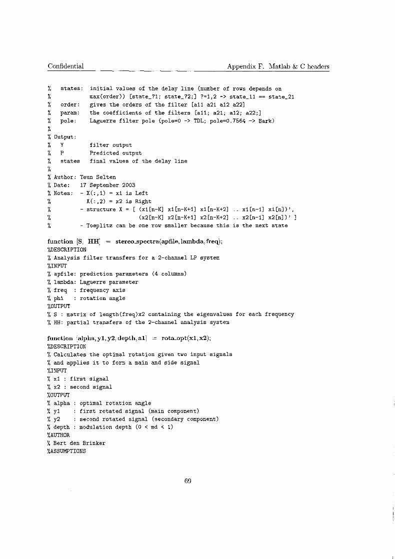
Confidential Appendix F. Matlab & C headers
% % % % % %
states:
order:
initial values of the delay line (number of rows depends on max(order)) [state_?!; state_?2;] ?=1,2 -> state_11 == state_21 gives the orders of the filter [a11 a21 a12 a22]
param: pole:
the coefficients of the filters [a11; a21; a12; a22;] Laguerre filter pole (pole=O -> TDL; pole=0.7564 ->Bark)
% Output: % y
% p
% states % % Author: % Date: % Notes: % % %
filter output Predicted output final values of the delay line
Teun Selten 17 September 2003 - X(:,1) = x1 is Left
X(:,2) = x2 is Right - structure X= [ (x1[n-K] x1[n-K+1] x1[n-K+2]
(x2[n-K] x2[n-K+1] x2[n-K+2] x1 [n-1] x1 [n]) ' , x2 [n-1] x2 [n]) ' ]
% Toeplitz can be one row smaller because this is the next state
function [S, HH] = stereo_spectra(apfile, lambda, freq); %DESCRIPTION % Analysis filter transfers for a 2-channel LP system %INPUT % apfile: prediction parameters (4 columns) % lambda: Laguerre parameter % freq frequency axis % phi rotation angle %OUTPUT % S : matrix of length(freq)x2 containing the eigenvalues for each frequency % HH: partial transfers of the 2-channel analysis system
function [alpha, yl, y2, depth, al] = rota_opt(xl, x2); %DESCRIPTION % Calculates the optimal rotation given two input signals % and applies it to form a main and side signal %INPUT % x1 : first signal % x2 : second signal %OUTPUT
optimal rotation angle % alpha % y1 % y2 % depth %AUTHOR
first rotated signal (main component) second rotated signal (secondary component) modulation depth (0 < md < 1)
% Bert den Brinker %ASSUMPTIONS
69

% x1 and x2 have the same size (vectors) % x1 and x2 are real-valued
function [g, sl, s2] = quanLsig_uni(sig, U, Levels); %DESCRIPTION % returns quantized signal and gains %INPUT % sig % u
signal segment size
% Levels: number of representation levels per sample %OUTPUT % g : quantization step per segment % s1 representation levels % s2 : quantized signal
function out= nonuniformquant(sig, U, levels); % Description: % Quantize the input signal with a non uniform quantizer
% % Input: % sig: the to be quantized input signal % U: block-length % levels: number op levels (must be an odd number)
% % Output: % out: quantized output signal % % Author: Teun Selten % Date: 16 January 2004 % Notes:
function [yl, y2] = rotate(xl, x2, alpha); % Description: % Rotates the given two input signals over alpha
% % Input: % x1 : first signal % x2 : second signal % alpha : rotation angle
% % Output: % y1 first rotated signal % y2 : second rotated signal
% % Author: Teun Selten % Date: 10 October 2003
70
Confidential

Confidential
% Notes: % from function rota_opt from Bert den Brinker % xi and x2 have the same size (vectors) % xi and x2 are real-valued
MatLab call for Mex-file
Appendix F. Matlab & C headers
out= dec_StereoJ.aguerre_fast(residual, apfile, datalength, pole, order);
% % Input:
% residual (i:length(input),2)
% apfile (i:(order *#segments) ,4)
% datalength data length of a segment
% pole laguerre pole
% order order of the synthesis filter
% % Output:
% out: (i:length(input),2)
71

Confidential
72

Bibliography
[1] Bauer, D. and D. Seitzer: "Statistical properties of high quality stereo signals in the time domain." IEEE Int. Conf. on Acoustics, Speech, and Signal Processing (ICASSP-89), Glasgow, Scotland. 23-26 May 1989. Vol 3, pp. 2045-2048.
[2] Bauer, D. and D. Seitzer: "Frequency domain statistics of high quality stereo signals." 86th AES Conv., Hamburg, Germany, February 1989. Preprint 2748.
[3] Baumgarte, F. and C. Faller: "Estimation of auditory spatial cues for binaural cue coding." IEEE Proc. ICASSP-02, Orlando, Florida USA. 13-17 May 2002. Vol. 2, pp 1801 - 1804, .
[4] Baumgarte, F. and C. Faller: "Binaural cue coding-Part I: Psychoacoustic fundamentals and design principles." IEEE Trans. on Speech f!3 Audio Processing, November 2003. Vol. 11, no. 6, pp 509 - 519.
[5] Biswas, A. and T. Selten, B. den Brinker: "Stability of the synthesis filter in stereo linear prediction." Proc. 15th ProRISC, Veldhoven, Netherlands, 25-26 November 2004.
[6] Blauert, J.: "Spatial Hearing; The psychophysics of human sound localization." The MIT Press, Cambridge England, 1997. ISBN 0-262-02413-6.
[7] Breebaart, J. and S. van de Par, A. Kohlrausch, E. Schuijers: "High-quality parametric spatial audio coding at low bitrates." 116th AES Conv., Berlin, Germany, May 2004.
Preprint 6072.
[8] den Brinker, A.C. and F. Riera-Palou: "Pure linear prediction." 115th AES Conv., New York, USA, September 2003. Preprint 5924
[9] den Brinker, A.C. and V. Voitishchuk, S.J.L. van Eijndhoven: "IIR-based pure linear prediction." IEEE Trans. on Speech f!3 Audio Processing, Januari 2004. Vol. 12, no. 1, pp
68- 75.
[10] Cambridge, P. and M. Todd: "Audio data compression techniques." 94th AES Conv., Berlin, Germany, March 1993. Preprint 3584.
[11] Dietz, M. and L. Liljeryd, K. Kjorling, 0. Kunz: "Spectral band replication, a Novel Approach in Audio Coding." 112th AES Conv., Munich, Germany, May 2002. Preprint
5553.
[12] Robert Bosch GmbH. "Verfahren zur redundanzreduktion." Inventors: Edler, B. and H. Fuchs. IPC8 H04B1/66. Deutsches Patentamt, DE 43 20 990 A 1. 5 January 1995.
73

Bibliography Confidential
[13] Robert Bosch GmbH. "Method for reducing data in a multi-channel data transmission" Inventors: Edler, B. and H. Fuchs. IPC6 H04B 1/66. United States Patent, US 5,511,093 A. 23 April 1996.
[14] Everest, F.A. and R. Streicher: "The new stereo soundbook." TAB Books McGraw-Hill, Blue Ridge Summit, PA, USA, 1992. ISBN 0-8306-3903-9.
[15] Faller, C. and F. Baumgarte: "Binaural cue coding: a novel and efficient representation of spatial audio." IEEE Proc. ICASSP '02, Orlando, Florida USA. 13-17 May 2002. Vol. 2, pp 1841 - 1844.
[16] Faller, C. and F. Baumgarte: "Binaural cue coding-Part II: schemes and applications." IEEE Trans. on Speech €3 Audio Processing, November 2003. Vol. 11 no. 6 pp 520- 531.
[17] Fuchs, H.: "Improving joint stereo audio coding by adaptive inter-channel prediction." IEEE Workshop on Appl. of Signal Processing to Audio and Acoustics, 17-20 October 1993. pp. 39-42.
[18] Fuchs, H.: "Improving MPEG audio coding by backward adaptive linear stereo prediction." 99th AES Conv., New York, October 1995. Preprint 4086.
[19] Garcia, J. and P. Gournay, R. Lefebvre: "Backward linear prediction for lossless coding of stereo audio." 116th AES Conv., Berlin, Germany, May 2004. Preprint 6076.
[20] Ghido, F.: "An asymptotically optimal predictor for stereo lossless audio compression." IEEE Computer Society Press Proc. Data Compression Conference DCC 2003, Snowbird, Utah, USA. 25-27 March 2003. pp 429.
[21] Harma, A. and U.K. Laine: "An experimental audio codec based on warped linear prediction of complex valued signals." IEEE ICASSP-97, Munich, Germany, 21-24 April 1997. vol 1, pp. 323-326.
[22] Harma, A. and U.K. Laine: "A comparison of warped and conventional linear predictive coding." IEEE Transactions on Speech €3 Audio Processing, July 2001. Vol 9, no 5, pp. 579-588.
[23] Herre, J. and E. Eberlein, K. Brandenburg: "Combined stereo coding." 93rd AES Conv., San Francisco, USA, October 1992. Preprint 3369.
[24] Herre, J. and K. Brandenburg, D. Lederer: "Intensity stereo coding." 96th AES Conv., Amsterdam, Netherlands, February 1994. Preprint 3379.
[25] Johnston, J.D.: "Perceptual transform coding ofwideband stereo signals." IEEE ICASSP-89, Glasgow, Scotland. 23-26 May 1989. Vol 3, pp. 1993-1996.
[26] Johnston, J.D. and A.J. Ferreira: "Sum-difference stereo transform coding." IEEE ICASSP-92, San Francisco, USA. 23-26 March 1992. Vol 2, pp. 569-572.
74

Confidential Bibliography
[27] Johnston, J. and J. Herre, M. Davis, U. Gbur: "MPEG-2 NBC audio- Stereo an multichannel coding methods." 101st AES Conv., Los Angeles, USA, November 1996. Preprint 4383.
[28] Jayant, N.S. and P. Noll: "Digital coding of waveforms. Principles and applications to speech and video." Prentice-Hall Inc, Englewood Cliffs, NJ, USA, 1984, ch. 6. ISBN 0-1321-1913-7.
[29] Kleijn, W.B. and K.K. Paliwal: "Speech coding and synthesis" Elsevier Science B. V., Amsterdam, Netherlands, 1995. ISBN 0-4448-2169-4
[30] Kuo, S.S. and Johnston, J.D.: "A study of why cross channel prediction is not applicable to perceptual audio coding." IEEE Signal Processing Letters, September 2001. Vol 8, no 9, pp. 245-247.
[31] Liebchen, T.: "Lossless audio using adaptive multichannel prediction." 113th AES Conv., Los Angeles, USA, October 2002. Preprint 5680.
[32] Lin, X. and R.A. Salami, R. Steele: "High quality audio coding using analysis-by-synthesis technique." IEEE Proc. ICASSP-91, Toronto, Canada. 14-17 April 1991. Vol.5, pp. 3617-3620.
[33] Liu, C.M. and W.C. Lee, Y.H. Hsiao: "M/S coding based on allocation entropy" Proc. 6th Conf. on Digital Audio Effects (DAFX-03), London, UK, 8-11 September 2003.
[34] van Loon, M.W.: "Very efficient coding of multi-channel audio." Philips PR-TN 2003/00428, 2003.
[35] Makhoul, J: "Linear prediction: A tutorial review." Proc. IEEE, April 1975. vol. 63, no. 4, pp. 561 - 580.
[36] Marple, S.L. Jr.: "Digital spectral analysis with applications." Prentice-Hall Inc, Englewood Cliffs, NJ, USA, 1987. Ch. 15. ISBN 0-1321-4149-3.
[37] Press, W.H. and B.P. Flannery, S.A. Teukolsky, W. T. Vetterling: "Numerical recipes in C: The art of scientific computing." Cambridge University Press, Cambridge, UK, 1988. ISBN 0-5214-3108-5.
[38] Singhal, S.: "High quality audio coding using multipulse LPC." IEEE Proc. ICASSP-90, Albuquerque, New Mexico USA. 3-6 April 1990. Vol.2, pp. 1101 - 1104.
[39] Smith, J.O. and J.S. Abel: "Bark and ERB bilinear transforms." IEEE Trans. on Speech Audio Processing, November 1999. Vol.6, pp. 697- 708.
[40] van der Waal, R.G. and R.N.J. Veldhuis: "Subband coding of stereophonic digital audio signals." IEEE ICASSP-91, Toronto, Canada. 14-17 April 1991. Vol 5, pp. 3601 - 3604.
[41] Wiggins, R.A. and E.A. Robinson: "Recursive solution to the multichannel filtering problem." Journal of Geophysical Research, 15 April 1965. Vol 70, No. 8, pp. 1885 - 1891.
75

Bibliography Confidential
[42] Whittle, P.: "On the fitting of multivariate autoregressions, and the approximate canonical factorization of a spectral density matrix." Biometrika, 1963. Vol. 50, pp. 129-134.
76