An Experimental and Numerical Investigation of Nonlinear Normal

Modes in Geometrically Nonlinear Structures

by

David Adam Ehrhardt

A dissertation submitted in partial fulfillment of the requirements for the degree of

DOCTOR OF PHILOSOPHY

(Engineering Mechanics)

at the

UNIVERSITY OF WISCONSIN-MADISON

2015

Date of final oral examination: 05/12/2015

The dissertation is approved by the following members of the Final Oral Committee:

Matthew S. Allen, Associate Professor, Engineering Physics

Daniel C. Kammer, Professor, Engineering Physics

Roderic S. Lakes, Professor, Engineering Physics

Melih Eriten, Assistant Professor, Mechanical Engineering

Timothy J. Beberniss, Aerospace Engineer, Air Force Research Laboratory

© Copyright by David A. Ehrhardt 2015

All Rights Reserved

i

Abstract

The design of modern structures operating in dynamic environments has placed emphasis

on light weight, flexible, and reusable structures, that lead to nonlinear force-displacement

relationships. In contrast, the test and analysis techniques that are available to guide designers are

fundamentally based on linear force-displacement relationships. The discrepancy between the

techniques needed and those that are available has motivated the pursuit of a better

understanding of how nonlinearity manifests in the field of structural dynamics. Although

nonlinear behavior can manifest in infinitely many ways, there are several features that can be

commonly observed in nonlinear structures. For example, the dynamic response amplitude can

be seen to depend on input energy or amplitude, the underlying (e.g. about some equilibrium)

linear modes of vibration become coupled at high dynamic response amplitudes, and higher

harmonics are generated in the response when the structure is subjected to a sinusoidal input. In

this context, new nonlinear test and analysis techniques should be developed to address the

generally observed behavior. This dissertation seeks to contribute to the nonlinear dynamic

testing of structures in two ways: first by presenting a means of collecting large number of DOF

measurements from the linear and nonlinear structure, and second by improving the means the

nonlinear structure is experimentally characterized with the improved implementation of the

nonlinear normal mode (NNM) concept in a testing environment.

The first contribution of this work to the state of the art extends the use of the spatially

dense measurement techniques of Three Dimensional-Digital Image Correlation (3D-DIC) and

Continuous-scan Laser Doppler Vibrometry (CSLDV) to nonlinear vibration measurements, and

presents the first experimental comparison of both techniques. 3D-DIC and CSLDV exhibit

limitations under certain loading conditions, deformation amplitudes, and complexity of spatial

ii

deformation as will be discussed in this dissertation. The full-field deformation information

available with 3D-DIC and CSLDV is especially beneficial when studying the thin walled

structures that are examined here. In linear response regimes, these structures are sensitive to

initial geometric imperfections which will effect the global dynamics of the structure. When only

a few measurement points are available, as with traditional test methods, there typically is not

enough information to tell what imperfections my be present and what effect they have on the

dynamics of a structure. In contrast, imperfections are clearly visible in full-field deformation

measurements. Furthermore, in nonlinear response regimes, these structures exhibit a nonlinear

coupling between linear normal modes, which is evident in the strength of the higher harmonics

and the deformation shape at each harmonic. This nonlinear coupling can be characterized using

the full-field deformation available at each harmonic.

This work's second contribution is the development of a new stepped-sine testing strategy

that allows the experimentalist to more easily isolate the nonlinear normal modes (NNMs) of the

structure of interest. NNMs are not necessarily synchronous periodic solutions of the

conservative nonlinear equations of motion (EOM) and can be arranged to compactly present

nonlinear behavior in frequency-energy plots (FEPs). A substantial amount of previous work

involving NNMs has focused on low dimension, or low degree of freedom (DOF), nonlinear

systems. This work seeks to exploit recent advancements that allow the computation of NNMs

for continuous structures with geometric nonlinearities. This is of particular interest since well

separated linear normal modes (LNMs) of such structures can become coupled, as evident by the

harmonic content observed in a nonlinear response regimes. This coupling causes an unexpected,

and possibly detrimental, change in the deformation of the structure. The harmonic content and

deformation shapes along FEP branches are key to the characterization of the nonlinear coupling

iii

of a structure's LNMs as a structure operates in nonlinear response regimes. This necessitates the

need for full-field measurements in the experimental identification of an NNM since the once

well separated LNMs are now commensurate at several harmonics in the response. Therefore, a

multi-harmonic input force is needed to isolate each LNM motion at each harmonic The required

input force is identified by tuning the fundamental frequency and amplitudes of the force at each

harmonic until the force/velocity plots of the positive and negative portions of the periodic cycle

overlay.

The use of full-field measurement techniques to isolate a structure's NNMs gives ample

spatial information when comparing test and analysis as a structure transitions from a linear

response regime to a nonlinear response regime. As will be shown, a structure's full-field

deformation provides valuable insight to the nonlinear deformation experienced by a structure.

Now that these methods can be used to identify the way in which the LNMs combine to produce

each NNM, a nonlinear experimental model can be identified from the measurements by

projecting the nonlinear deformation onto the structures LNMs. This experimental model allows

one to compare the actual performance of the structure with numerically calculated modal

models in much more detail and is shown to help guide model updating efforts.

iv

Acknowledgements

My path to a Ph.D. has included 22 years focusing on my education. Teachers and

professors have been central to my success and require my deepest gratitude. First and foremost,

I would like to thank my advisor, Dr. Matt Allen, for his assistance and patience during my time

at UW-Madison. He support and guidance have further deepened my understanding and desire to

pursue my research path. I would also like to thank my previous advisor, Dr. Jorge Abanto-

Bueno, for setting me on my current path to a Ph.D. I would not have achieved my current level

of academic success without continuous encouragement from my former teacher, Mr. Roger

Leach, who has always pushed me to continue to learn.

I would also like to extend my gratitude to my Ph.D. committee for taking the time to

review the material in this dissertation and provide feedback. I'd like to extend a special thanks to

Tim Beberniss for his help in the lab and support when using high speed 3D-DIC for all of my

summers spent in Ohio.

I have had the pleasure of meeting many talented colleagues throughout my time spent at

UW-Madison and Bradley University. These researchers are too numerous to list, but have been

key to the development of this work.

I am grateful for receiving financial support from the Wisconsin Alumni Research

Foundation and the Morgridge Distinguished Graduate Fellowship as well as the J. Gordon

Baker Fellowship.

Finally, I would like to thank my family and friends for all of their support and

encouragement during my time as a student. Without their reinforcement I probably would not

be where I am today. My wife and parents have always been the a positive force throughout my

academic career and I am eternally grateful.

v

Abbreviations

3D-DIC Three-Dimensional Digital Image Correlation

CSLDV Continuous-scan Laser Doppler Vibrometry

DOF Degree-of-freedom

EOM Equations of Motion

FEA Finite Element Analysis

FEM Finite Element Model

FRF Frequency Response Function

LNM Linear Normal Mode

MAC Modal Assurance Criterion

MIF Mode Indicator Function

MO Mode Orthogonality

NNM Nonlinear Normal Mode

V&V Verification and Validation

vi

Contents

Abstract........................................................................................................................................... i

Acknowledgements ...................................................................................................................... iv

Abbreviations ................................................................................................................................ v

Contents ........................................................................................................................................ vi

1 Introduction........................................................................................................................... 1

1.1 Motivation ......................................................................................................................... 1

1.2 Full-Field Measurement Techniques ................................................................................. 6

1.3 Nonlinear Normal Modes ................................................................................................ 10

1.4 Proposed Test and Analysis Methodology ...................................................................... 17

1.5 Scope of the Dissertation................................................................................................. 20

2 The use of Continuous-scan Laser Doppler Vibrometry and 3D Digital Image

Correlation for Full-Field Linear and Nonlinear Measurements .......................................... 22

2.1 Introduction ..................................................................................................................... 22

2.2 Continuous-scan Laser Doppler Vibrometry................................................................... 22

2.3 Three-Dimensional Digital Image Correlation................................................................ 26

2.4 Experimental Setup.......................................................................................................... 30

2.5 Measurement of Linear and Nonlinear Response of a Clamped-Clamped Flat Beam.... 33

2.5.1 Beam Description............................................................................................... 33

2.5.2 Linear Response Comparison............................................................................. 36

2.5.3 Nonlinear Response Comparison ....................................................................... 40

2.6 Measurement of Linear and Nonlinear Response of a Clamped Flat Plate..................... 43

2.6.1 Flat Plate Structure ............................................................................................. 43

vii

2.6.2 Linear Plate Response Comparison.................................................................... 46

2.6.3 Nonlinear Plate Response Comparison .............................................................. 48

2.7 Summary.......................................................................................................................... 51

3 Experimental Identification of Nonlinear Normal Modes .............................................. 54

3.1 Introduction ..................................................................................................................... 54

3.2 Linear Normal Modes...................................................................................................... 58

3.2.1 Introduction ........................................................................................................ 58

3.2.2 Measuring Linear Normal Modes with Force Appropriation ............................ 59

3.3 Nonlinear Normal Modes ................................................................................................ 62

3.3.1 Introduction ........................................................................................................ 62

3.3.2 Numerical Example of NNM ............................................................................. 63

3.3.3 Measuring NNMs with Force Appropriation ..................................................... 67

3.3.3.1 Theoretical Development ................................................................................... 67

3.3.3.2 Numerical Example of Stepped Sine Measurement of NNM............................ 70

3.3.3.3 Numerical Example of Free Decay Measurement of NNM............................... 74

3.3.3.4 Comparison of NNM Measurement Methods.................................................... 77

3.4 Application to Clamped-Clamped Flat Beam with Geometric Nonlinearity .................. 78

3.4.1 Flat Beam Description........................................................................................ 78

3.4.2 Experimental Setup ............................................................................................ 80

3.4.3 Flat Beam Experimental Results ........................................................................ 82

3.4.3.1 Effect of Magnetic Driver on the Dynamics of the Beam.................................. 82

3.4.3.2 Voltage-Velocity plots and phase lag of harmonics........................................... 84

3.4.3.3 Experimental Frequency-Amplitude Results ..................................................... 89

viii

3.4.3.4 Full-Field Deformation Shapes .......................................................................... 94

3.5 Application to Axi-symmetric Curved Plate with Geometric Nonlinearity .................... 96

3.5.1 Plate Description ................................................................................................ 96

3.5.2 Plate NNM Calculation ...................................................................................... 99

3.5.3 Plate NNM Measurement................................................................................. 101

3.6 Summary........................................................................................................................ 105

4 Model Updating and Validation using Experimentally Measured Linear and

Nonlinear Normal Modes ......................................................................................................... 107

4.1 Introduction ................................................................................................................... 107

4.2 Modeling Considerations............................................................................................... 108

4.3 Model updating of Clamped-Clamped Flat Beam with Geometric Nonlinearity ......... 109

4.3.1 Flat Beam Description...................................................................................... 109

4.3.2 Flat Beam Linear Comparison ......................................................................... 110

4.3.3 Flat Beam Nonlinear Comparison.................................................................... 112

4.4 Model updating of Clamped-Clamped Curved Beam with Geometric Nonlinearity.... 115

4.4.1 Curved Beam Description ................................................................................ 115

4.4.2 Curved Beam Linear Comparison.................................................................... 116

4.4.3 Curved Beam Nonlinear Comparison .............................................................. 118

4.5 Summary........................................................................................................................ 120

5 Summary............................................................................................................................ 122

5.1 Continuous-scan Laser Doppler Vibrometry and Three Dimensional-Digital Image

Correlation .............................................................................................................................. 122

5.2 Experimental Identification of Nonlinear Normal Modes............................................. 124

ix

5.3 Model Updating and Validation using Experimentally and Numerically Determined

Linear and Nonlinear Normal Modes ..................................................................................... 125

6 Future Work...................................................................................................................... 126

6.1 Characterization and Optimization of Experimental Setup for Continuous-scan Laser

Doppler Vibrometry and Three Dimensional-Digital Image Correlation .............................. 126

6.2 Experimental Identification of Nonlinear Normal Modes............................................. 126

6.3 Update Models using Nonlinear Normal Modes........................................................... 127

6.4 Model Validation using Nonlinear Measured and Simulated Responses...................... 127

Acknowledgements ................................................................................................................... 128

Appendix – Publications of PhD work.................................................................................... 129

References .................................................................................................................................. 131

1

1 Introduction

1.1 Motivation

The testing and analysis of a machine or structure are key steps to support decision

making during the design process. For instance, complementary results from a test and an

analysis are used to identify areas of uncertainty between the physical machine or structure and

the mathematical model used to describe it. Alternatively, individual results from an analysis are

used when the machine or structure of interest operates outside the ranges of available testing

facilities. Similarly, individual results from a test are used when the machine or structure

operates within knowledge gaps of analysis methods. In current practice, an analytical model

will not typically be used without first comparing its response to tests on the structure of interest;

otherwise unexpected errors can distort results and lead to incorrect design decisions. In this

context, formal guidelines have been created to aid in the establishment of a suitable comparison

between test and analysis under the title of model validation, which is a branch of Verification

and Validation (V&V) [1]. Model validation seeks to answer the question, "Are we solving the

correct equations?" by comparing the physical and modeled structure under expected loading

conditions [2]. Prior to model validation, a model calibration is performed, where fundamental

properties of the physical and modeled structure are compared with the goal of determining the

correct model order, selected structural parameters, and quantifying uncertainty within the

physical and modeled structure. Due to the overlapping relationship between test and analysis

throughout the model validation process, advancements in testing techniques are motivated by

advances in analysis methods, and visa-versa.

2

When considering the field of structural vibrations, a substantial amount of work has built

model calibration metrics around dynamic linear force-displacement relationships [3-6]. These

metrics hinge on the quantification of invariant dynamic properties inherent to the linear normal

modes (LNMs) of a structure (e.g. resonant frequencies and mode shapes), and include resonant

frequency error, frequency response functions, modal assurance criterion (MAC), etc. [7].

Physically, LNMs represent uncoupled synchronous motions of a structure defined by its

undamped free vibration characteristics. Mathematically, LNMs represent non-trivial solutions to

the conservative unforced equations of motion (EOM):

( ) ( ) 0=+ tt KxxM && (1.1)

For an n degree of freedom (DOF) system, M is an n x n mass matrix, K is an n x n

stiffness matrix, x(t) is an n x 1 vector of the displacement of the system, and ẍ(t) is an n x 1

vector of the acceleration of the system. Assuming harmonic motion, ( ) ( )tt ωcosXx = , the EOM

can be recast as an eigenvalue/vector problem:

( ) 02

=− ΦMωK n

(1.2)

Where the n x 1 eigenvalues (ωn) and the n x n eigenvectors (Φ) define the LNMs of a

structure. For a linear structure such as this, the LNMs are amplitude invariant, decouple the

EOM due to their orthogonality, and can be used to find an analytical solution for the free and

forced vibrations of the structure through the superposition principle. Exploiting the properties of

LNMs in structural vibrations has been the cornerstone to developing test and analysis

techniques in the areas of finite element model updating [4], experimental modal analysis [5],

and model reduction [8].

3

A central idea behind these techniques is the use of a truncated set of dynamically

important LNMs to define the structure's global free or forced deformations and guide the model

calibration. It is left to the engineer to decide which set of LNMs to measure in a test or use in an

analysis, and there are several techniques to aid in this decision [8]. The number of LNMs

included in the truncated set further defines the minimum number and location of measured or

modeled degrees of freedom (DOF). In current practice, the number of DOF within a test is

typically tens to hundreds, while analysis methods can produce millions. In standard practice, the

data available from an analysis is reduced or interpolated to compare with test data. The

assumption is made that the reduced DOF used in an experiment can capture the LNMs of a

structure well. However, structures whose dynamics are sensitive to the definition of the initial

static equilibrium (e.g. thin beams and plates) can experience variations in LNMs that are not

captured by the truncated set of DOF, underlining the need for more experimental measurement

DOF. A second assumption this process makes is that the physical structure behaves linearly,

justifying the use of LNMs as a basis for the model calibration process. However, the linearity

assumption is well known as the exception rather than the rule for real world structures, and the

increasing desire to design nonlinear structures has accentuated the short comings of using

LNMs as a basis for nonlinear model calibration. This dissertation seeks to address these model

calibration shortcomings in two ways: first by presenting a means of collecting spatially dense

measurements from the linear and nonlinear structure, and second by developing a new stepped-

sine testing strategy that allows the experimentalist to more easily isolate the nonlinear normal

modes. These objectives are explained in detail below.

The total available number of DOF in a test is presently limited by the use of traditional

discrete sensors (e.g. accelerometers, linearly varying displacement transducers, and strain

4

gauges). The number of such sensors that can be used in a test is restricted by cost and their

effect on the structural response. For example, when a large number of such sensors are attached

to the structure, the mass loading effects will decrease the natural frequencies and distort the

mode shapes of a structure. Advanced measurement techniques, such as Continuous-scan Laser

Doppler Vibrometry (CSLDV) [9] and high speed Three Dimensional-Digital Image Correlation

(3D-DIC) [10], have been developed to obtain more spatial information of a structure's

deformation while reducing the effect on the response of a structure. Both techniques are

relatively new and have not been effectively compared as a structure deforms from linear to

nonlinear response regimes in a vibratory environment. Additionally, the combination of

CSLDV and 3D-DIC within the framework of a nonlinear normal mode, which is expounded

upon in the next paragraph, provides the information needed to diagnose how the LNMs are

coupled as a response transitions from a linear to a nonlinear response regime.

The generalization of a mode of vibration to accommodate nonlinear responses has lead

to the definition of nonlinear normal modes (NNMs). Rosenberg [11] first defined a NNM as a

synchronous motion of the nonlinear system which provided a direct extension of the LNM

concept. This definition has been broadened to include not necessarily synchronous periodic

motions of the conservative nonlinear equations of motion (EOM) [12, 13]. The extended

definition allows NNMs to contain phenomena including bifurcations [12], internal resonances

[14], and strong dependence on the amplitude of the response [15]. The primary body of work on

NNMs has been on their analytical and numerical calculation for low DOF systems [13]. Few

works have been published in which an NNM of a physical structure has been isolated

experimentally [16, 17], perhaps because of the complex dynamics associated with a NNM

response. Over the past several decades, phase separation [18-20], and phase resonance

5

techniques [21, 22], have been explored to experimentally characterize a nonlinear structure. The

development of these methods has relied on the assumption that the damping observed in a

structure is well defined; however, this is not generally the case for real structures. By

approaching the measurement of a NNM as a stepped-sine test, an appropriation vector can be

realized at each subsequent step removing the need for this damping assumption. However, the

multi-harmonic nature of the response makes determining the correct appropriation vector

difficult in practice. This thesis proposes a means of isolating an NNM, and shows that by simply

monitoring a force-velocity plot (which is easy to implement in real time) one can tune the

frequency and harmonic amplitudes in the force to isolate an NNM.

For the purposes of this thesis, the final goal of the comparison of test and analysis is to

create a calibrated model that captures the dynamics of a structure in the response regions of

interest which can then be applied to other loading conditions not considered in a physical test

scenario. If a structure behaves linearly, the accurate modeling of LNMs over a frequency range

of interest can give the designer confidence in the predicted structural deformation in a dynamic

environment. The use of LNMs to update the underlying analytical model is well established in

the field of structural dynamics [4]. As previously discussed, the dynamic test and analysis

procedures built on LNMs cannot be directly applied to the determination of NNMs; however, it

is useful to first determine the LNMs (e.g. about some equilibrium) of the nonlinear structure to

be used as a starting point when updating the nonlinear model. This now becomes the first step in

the model calibration process used for this dissertation shown in Fig. 1.1. LNMs define an

unambiguous model of the structure in its initial state providing an anchor for the model

calibration. With the fully updated linear models, the NNMs can be calculated using an assumed

initial form of the nonlinearity. Alternatively, the form of the nonlinearity can be determined

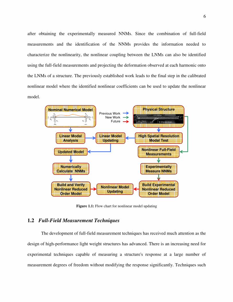
6

after obtaining the experimentally measured NNMs. Since the combination of full-field

measurements and the identification of the NNMs provides the information needed to

characterize the nonlinearity, the nonlinear coupling between the LNMs can also be identified

using the full-field measurements and projecting the deformation observed at each harmonic onto

the LNMs of a structure. The previously established work leads to the final step in the calibrated

nonlinear model where the identified nonlinear coefficients can be used to update the nonlinear

model.

Linear Modal

Analysis

High Spatial Resolution

Modal Test

Experimentally

Measure NNMs

Nominal Numerical Model

KT KT

KAKA

Kθ

Kθ

Numerically

Calculate NNMs

Physical Structure

Build and Verify

Nonlinear Reduced

Order Model

Build Experimental

Nonlinear Reduced Order Model

Nonlinear Full-Field

MeasurementsUpdated Model

Linear Model

Updating

Previous Work

New Work

Future

Nonlinear Model Updating

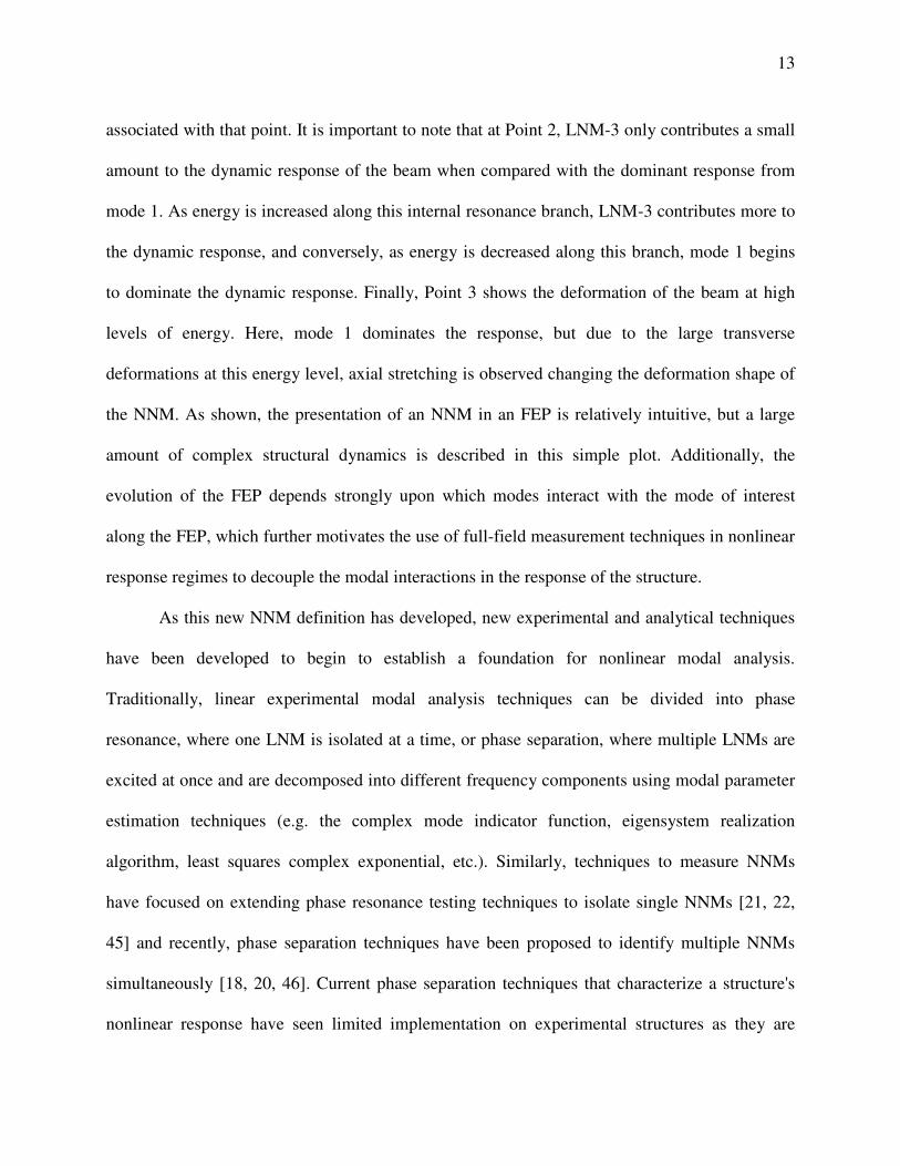
Figure 1.1: Flow chart for nonlinear model updating

1.2 Full-Field Measurement Techniques

The development of full-field measurement techniques has received much attention as the

design of high-performance light weight structures has advanced. There is an increasing need for

experimental techniques capable of measuring a structure's response at a large number of

measurement degrees of freedom without modifying the response significantly. Techniques such

7

as Continuous-scan Laser Doppler Vibrometry (CSLDV) and high-speed Three Dimensional-

Digital Image Correlation (3D-DIC) have been developed to meet this need. Both CSLDV and

high-speed 3D-DIC are capable of measuring the response at thousands of points across the

surface of a structure. However, these techniques involve additional processing to extract

velocities or displacements when compared with traditional measurement techniques.

A Laser Doppler Vibrometer (LDV) is a device capable of measuring the velocity of a

single stationary point on the surface of a deforming structure by calculating the Doppler shift of

the reflected laser light. CSLDV extends the LDV concept by continuously moving the laser by a

known pattern across the surface of a deforming structure instead of dwelling at a single location.

The motion of the laser requires additional consideration in the experimental setup since, the

quality of the reflected laser signal is key to the accurate measurement of velocity and the

measurement grid is dependent on the selected scan pattern. Measurements with CSLDV also

require an additional processing step when compared with LDV measurements because the

continuously moving measurement point requires the measurement to be described by a linear

time-varying or, more specifically, linear time-periodic dynamic model [23]. The benefit

provided by the continuously moving measurement point is an increased measurement resolution

with drastically decreased measurement time when compared with the conventional approach of

individually dwelling at a measurement location for a prescribed length of time. Various

algorithms have been devised to determine the mode shapes of a structure along a continuously

moving laser scan path. For example, Ewins et al. treated the operational deflection shape as a

polynomial function of the moving laser position [9, 24-27]. They showed that sideband

harmonics appear in the measured spectrum separated by the scan frequency, and that the

amplitudes of the sidebands can be used to determine polynomial coefficients describing the

8

deformation shape. Allen et al. later presented a lifting approach for impulse response

measurements [28, 29]. The lifting approach groups the responses at the same location along the

laser path. Hence, the lifted responses appear to be from a set of pseudo sensors attached to the

structure, allowing conventional modal analysis routines to extract modal parameters from the

CSLDV measurements. Recently, Linear Time Periodic (LTP) system theory has been used to

derive modal identification algorithms that parallel traditional linear time invariant (LTI) system

theory [30-33]. Therefore, a structure's dynamic response due to virtually any type of loading

(measured or unmeasured) can be measured over the laser scan path through the use of the input-

output transfer functions and power spectrums similar to classical LTI modal analysis.

2D-DIC uses a single camera to match planar deformations throughout a series of

captured images and has been widely used in fracture mechanics. 3D-DIC extends this idea to all

three spatial dimensions by adding a second camera and a second set of captured images of the

deforming surface. Through a series of coordinate transformations, the full-field 3D deformation

of a structure is measured [10]. When considering the application of 3D-DIC to the dynamic

measurements of structures undergoing large deformation, issues such as lighting, camera

placement, field and depth of view for the physical setup are critical to obtain accurate

measurements. For sample rates greater than 100 fps, these considerations require measurements

to be obtained through an additional step of post processing. Schmidt et al. [34] presented early

work on the use of high-speed digital cameras to measure deformation and strain experienced by

test articles under impact loadings. Similarly, Tiwari et al. [35] used two high-speed CMOS

cameras in a stereo-vision setup to measure the out of plane displacement of a plate subjected to

a pulse input. The transient deformations measured compared favorably with work previously

published and showed the capability of the 3D-DIC system in a high-speed application, although

9

over a short time history. Niezrecki et al. [36], Helfrick et al. [37], and Warren et al. [38]

measured mode shapes of several structures using discrete 3D-DIC in a frequency range below

200Hz. Niezrecki et al. and Helfrick et al. also combined accelerometers, vibrometers, and

dynamic photogrammetry to compare the measured mode shapes and natural frequencies

obtained with 3D-DIC. Each technique provided complementary results showing the capability

of 3D-DIC, although 3D-DIC was not processed along the entire surface of the structure. Abanto

Bueno et al. [39], Beberniss and Ehrhardt [40, 41], and Ehrhardt et al. [42, 43] explored

measurement error in full-full field 3D-DIC vibration measurements in frequency ranges up to

1000Hz made on structures subjected to random and sinusoidal loading. In such environments

3D-DIC provided accurate 3D deformation fields of the structures investigated. Due to the

extended duration of at test to obtain higher frequency deformations, handling the large amount

of data in conjunction with the image files limits the use of 3D-DIC in vibration measurements.

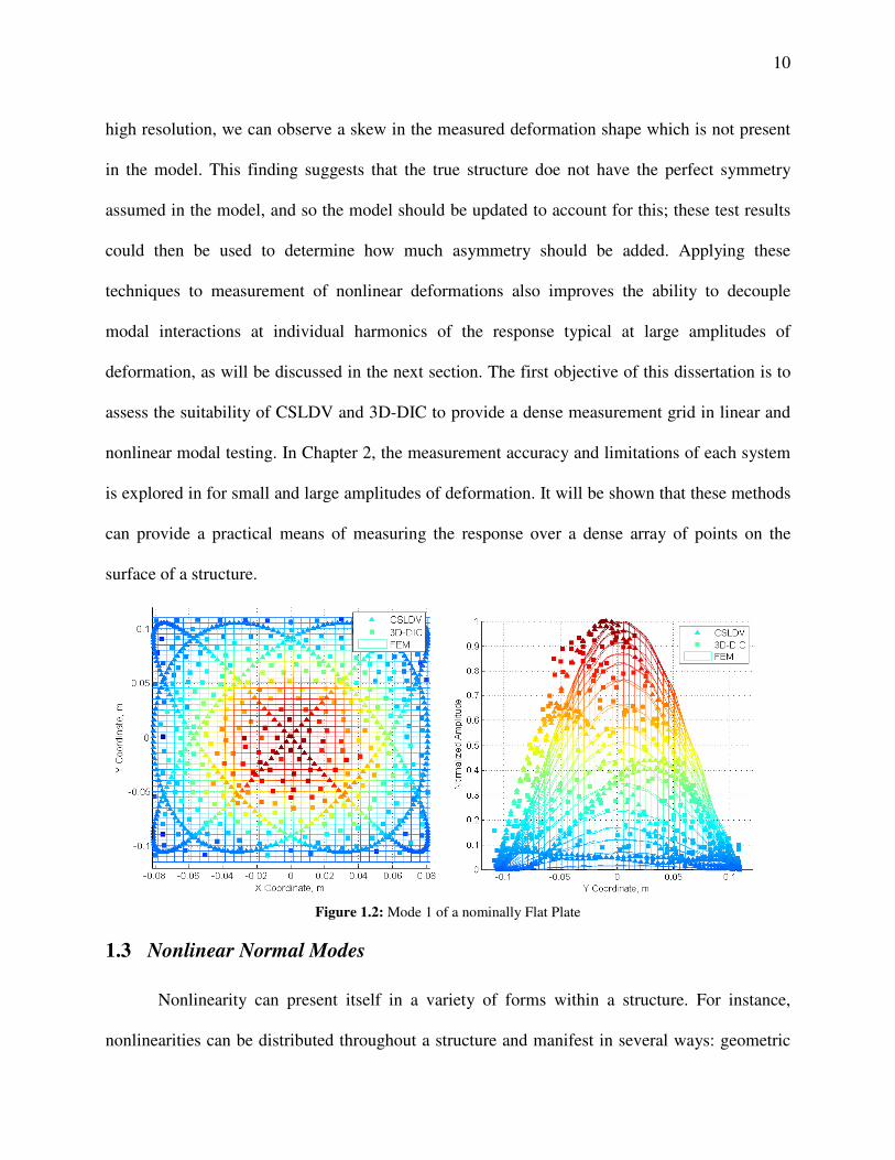
These techniques provide an unprecedented number of measured DOF, allowing one to

make a much more informative comparison between test and analysis and provides insight to

variations of the underlying physical structure (e.g. variations in initial conditions). This is

illustrated in Fig. 1.2, where the first mode of a finite element model of a flat plate considered in

this work is overlaid on measurements of the first mode of the flat plate using CSLDV (shown

with triangles) and 3D-DIC (shown with squares). For reference between the two plots, the

amplitude of deformation is color coded from low (blue) to high (red) amplitude. These results

will be discussed in more detail later, but for now it is interesting to note that CSLDV and 3D-

DIC provide a comparable number of DOF between the measured and calculated mode shape. It

is also of note that the measurement grid differences between CSLDV and 3D-DIC are inherent

to their implementation, as will be discussed in Chapter 2. Because these methods provide such

10

high resolution, we can observe a skew in the measured deformation shape which is not present

in the model. This finding suggests that the true structure doe not have the perfect symmetry

assumed in the model, and so the model should be updated to account for this; these test results

could then be used to determine how much asymmetry should be added. Applying these

techniques to measurement of nonlinear deformations also improves the ability to decouple

modal interactions at individual harmonics of the response typical at large amplitudes of

deformation, as will be discussed in the next section. The first objective of this dissertation is to

assess the suitability of CSLDV and 3D-DIC to provide a dense measurement grid in linear and

nonlinear modal testing. In Chapter 2, the measurement accuracy and limitations of each system

is explored in for small and large amplitudes of deformation. It will be shown that these methods

can provide a practical means of measuring the response over a dense array of points on the

surface of a structure.

Figure 1.2: Mode 1 of a nominally Flat Plate

1.3 Nonlinear Normal Modes

Nonlinearity can present itself in a variety of forms within a structure. For instance,

nonlinearities can be distributed throughout a structure and manifest in several ways: geometric

11

nonlinearity (e.g. large deformations of flexible elastic continua such as beams and plates),

inertia nonlinearity (e.g. Coriolis accelerations of translating and rotating bodies), material

nonlinearity (e.g. nonlinear stress/strain relationships), or damping nonlinearity (e.g. distributed

fluid layer on structure surface). Other nonlinearities occur at discrete locations such as a joint

nonlinearity (e.g. dry friction and stick/slip from relative motion of joint) and vibro-impacts (e.g.

clearance constraints). Presently, there has been no general test and analysis methodology that

can be applied to all nonlinearities since each type of nonlinearity has a distinct mathematical

form and give rise to vastly different physics. However, there are several phenomena that are

common to many types of nonlinear structures including response amplitude dependence,

coupling between linear modes of vibration, and the generation of integer related higher-

harmonic responses. The nonlinear normal mode (NNM) concept extends many of the

conceptual benefits of linear normal modes (LNMs) to nonlinear systems. Similar to the LNMs

previously introduced in Eqns. (1.1) and (1.2), the definition of NNMs is rooted in the

conservative homogeneous EOM, which can be written as follows:

( ) ( ) ( )txtt ,nlfKxxM ++&& (1.3)

Where fnl represents the nonlinear stiffness coupling between the displacements which is

of particular interest for this dissertation. A NNM is defined as not necessarily synchronous

solutions of the conservative nonlinear EOM. The extended definition allows NNMs to contain

phenomena including bifurcations [12], internal resonances [14], and strong dependence on the

amplitude of the response [15]. Due to the complex nature of the dynamics included in a NNM, a

graphical depiction of the NNMs is key to their use in test and analysis of nonlinear structures.

The use of a frequency-energy plot (FEP) has become relatively standard in the examination of

12

NNMs [44] and groups 'families' of NNMs with similar dynamic properties together which aids

the comparison of experimentally measured and numerically calculated NNMs.

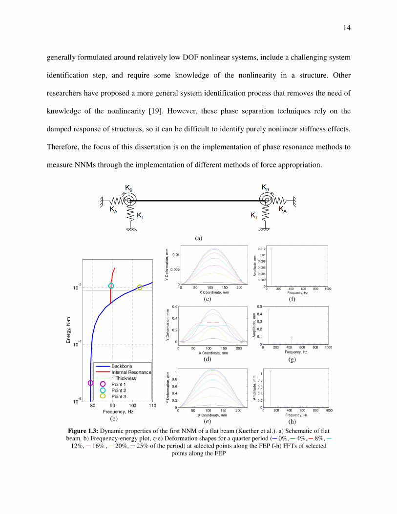
For example, the dynamics of the first 'family' of NNMs of the clamped-clamped flat

beam investigated in this dissertation are shown in Fig. 1.3. The FEP in Fig. 1.3b contains two

'families' of NNMs. The first family, shown in blue, is the nonlinear continuation of LNM-1 and

is typically termed the backbone branch or NNM-1. Along this backbone, it is observed that the

fundamental frequency exhibits a spring hardening dependence on the total energy of the

response of the beam or in other words, NNM-1 exhibits an increase of the fundamental

frequency vibration with increasing energy. The second 'family' of NNMs, shown in red, is a

bifurcation from the NNM-1 backbone and pertains to a 5:1 nonlinear harmonic coupling in the

response of the beam. This coupling is known to arise because of interactions between the

underlying linear modes of the structure; specifically this branch pertains to a coupling between

LNM-1 and LNM-3. On this branch, the deformation shape is a combination of the deformations

of the underlying LNMs and higher harmonics in the temporal response are key to understanding

this nonlinear coupling.

The dynamic characteristics of these NNMs can be further understood though the

examination of the deformation of the beam throughout a quarter period of response (Figs. 1.3c-

e) and the Fourier coefficients of center point beam deflection over a period of the response

(Figs. 1.3f-h) at selected points along the frequency-energy plot (FEP). Beginning in the linear

region of the response, Point 1 shows a LNM-1 deformation of the beam, which is confirmed in

the deformation shape and Fourier coefficients of the point. Point 2 refers to the response of the

5:1 harmonic interaction, which contains a primarily LNM-3 deformation of the beam. This can

again be confirmed through the examination of the deformation shape and Fourier coefficients

13

associated with that point. It is important to note that at Point 2, LNM-3 only contributes a small

amount to the dynamic response of the beam when compared with the dominant response from

mode 1. As energy is increased along this internal resonance branch, LNM-3 contributes more to

the dynamic response, and conversely, as energy is decreased along this branch, mode 1 begins

to dominate the dynamic response. Finally, Point 3 shows the deformation of the beam at high

levels of energy. Here, mode 1 dominates the response, but due to the large transverse

deformations at this energy level, axial stretching is observed changing the deformation shape of

the NNM. As shown, the presentation of an NNM in an FEP is relatively intuitive, but a large

amount of complex structural dynamics is described in this simple plot. Additionally, the

evolution of the FEP depends strongly upon which modes interact with the mode of interest

along the FEP, which further motivates the use of full-field measurement techniques in nonlinear

response regimes to decouple the modal interactions in the response of the structure.

As this new NNM definition has developed, new experimental and analytical techniques

have been developed to begin to establish a foundation for nonlinear modal analysis.

Traditionally, linear experimental modal analysis techniques can be divided into phase

resonance, where one LNM is isolated at a time, or phase separation, where multiple LNMs are

excited at once and are decomposed into different frequency components using modal parameter

estimation techniques (e.g. the complex mode indicator function, eigensystem realization

algorithm, least squares complex exponential, etc.). Similarly, techniques to measure NNMs

have focused on extending phase resonance testing techniques to isolate single NNMs [21, 22,

45] and recently, phase separation techniques have been proposed to identify multiple NNMs

simultaneously [18, 20, 46]. Current phase separation techniques that characterize a structure's

nonlinear response have seen limited implementation on experimental structures as they are

14

generally formulated around relatively low DOF nonlinear systems, include a challenging system

identification step, and require some knowledge of the nonlinearity in a structure. Other

researchers have proposed a more general system identification process that removes the need of

knowledge of the nonlinearity [19]. However, these phase separation techniques rely on the

damped response of structures, so it can be difficult to identify purely nonlinear stiffness effects.

Therefore, the focus of this dissertation is on the implementation of phase resonance methods to

measure NNMs through the implementation of different methods of force appropriation.

(a)

0 50 100 150 2000

0.005

0.01

X Coordinate, mm

Y D

efo

rmation,

mm

(c)

0 200 400 600 800 10000

0.002

0.004

0.006

0.008

0.01

0.012

Frequency, Hz

Am

plitu

de

, m

m

(f)

0 50 100 150 200

0

0.2

0.4

0.6

X Coordinate, mm

Y D

efo

rmati

on,

mm

(d)

0 200 400 600 800 10000

0.1

0.2

0.3

0.4

0.5

Frequency, Hz

Am

pli

tud

e,

mm

(g)

10-6

10-4

10-2

80 90 100 110

Frequency, Hz

Ene

rgy,

N-m

Backbone

Internal Resonance

1 Thickness

Point 1

Point 2

Point 3

(b)

0 50 100 150 2000

0.2

0.4

0.6

0.8

1

X Coordinate, mm

Y D

efo

rmati

on,

mm

(e)

0 200 400 600 800 10000

0.2

0.4

0.6

0.8

1

Frequency, Hz

Am

pli

tud

e,

mm

(h)

Figure 1.3: Dynamic properties of the first NNM of a flat beam (Kuether et al.). a) Schematic of flat

beam. b) Frequency-energy plot, c-e) Deformation shapes for a quarter period (─ 0%, ─ 4%, ─ 8%, ─

12%, ─ 16% , ─ 20%, ─ 25% of the period) at selected points along the FEP f-h) FFTs of selected

points along the FEP

15

Atkins et al. [22] presented a force appropriation of nonlinear systems (FANS) method

using a multi-point multi-harmonic force vector to isolate a linear normal mode (LNM) of

interest. This permits the direct nonlinear characteristics of the isolated mode to be calculated

without modal coupling terms. Peeters et al. [16, 21] showed that a multi-point multi-harmonic

sine wave could isolate a single NNM. For application to real world structures, it was then

demonstrated that a single-point single harmonic force could be used to isolate a response in the

neighborhood of a single NNM with good accuracy [16, 47]. In these investigations, once phase

lag quadrature was met, the input force was turned off and the response allowed to decay tracing

the backbone of the NNM. Building off of this work, Ehrhardt et al. [48] used step sine testing to

measure the response around a specific NNM and at several input forcing levels leading to

nonlinear frequency response functions (FRFs). From these FRFs, responses in the neighborhood

of the NNM can be isolated from measured responses. Similarly, using manually tuned stepped

sine excitation, Ehrhardt et al. [45] showed the ability to isolate a NNM through incrementally

increasing force levels and adjusting the frequency of the input force to experimentally measure

a NNM. This method drastically reduces the amount of data measured while isolating a NNM,

making the implementation of full-field measurements feasible.

For the calculation of nonlinear normal modes (NNMs), several analytical and numerical

techniques are available. Analytical techniques, such as the method of multiple scales [12, 13,

49, 50] and the harmonic balance approach [15], are typically restricted to structures where the

equations of motion are known in closed form, so analysis is limited to simple geometries. This

dissertation is focused on realistic (e.g. FEM) models for a structure where the analytical

methods are not usually practical. To expand the calculation of NNMs to more complex

geometries, asymptotic [51] and continuation based [12, 13, 52] numerical methods have been

16

developed to calculate NNMs of discrete systems. Recently, numerical methods based on

continuation have also been extended to calculate NNMs of larger scale structures [52-54] using

MATLAB® coupled with a commercial FEA code such as Abaqus®. Of interest for this

dissertation, Kuether et al. [52] proposed a direct method to compute the NNMs of full-ordered

models termed the applied modal force (AMF) algorithm. Similarly, Allen et al. [55] used

nonlinear reduced order models (NLROMs) to calculate the NNMs of a structure, allowing

NNMs to be calculated of more complex structures at a modest computational cost.

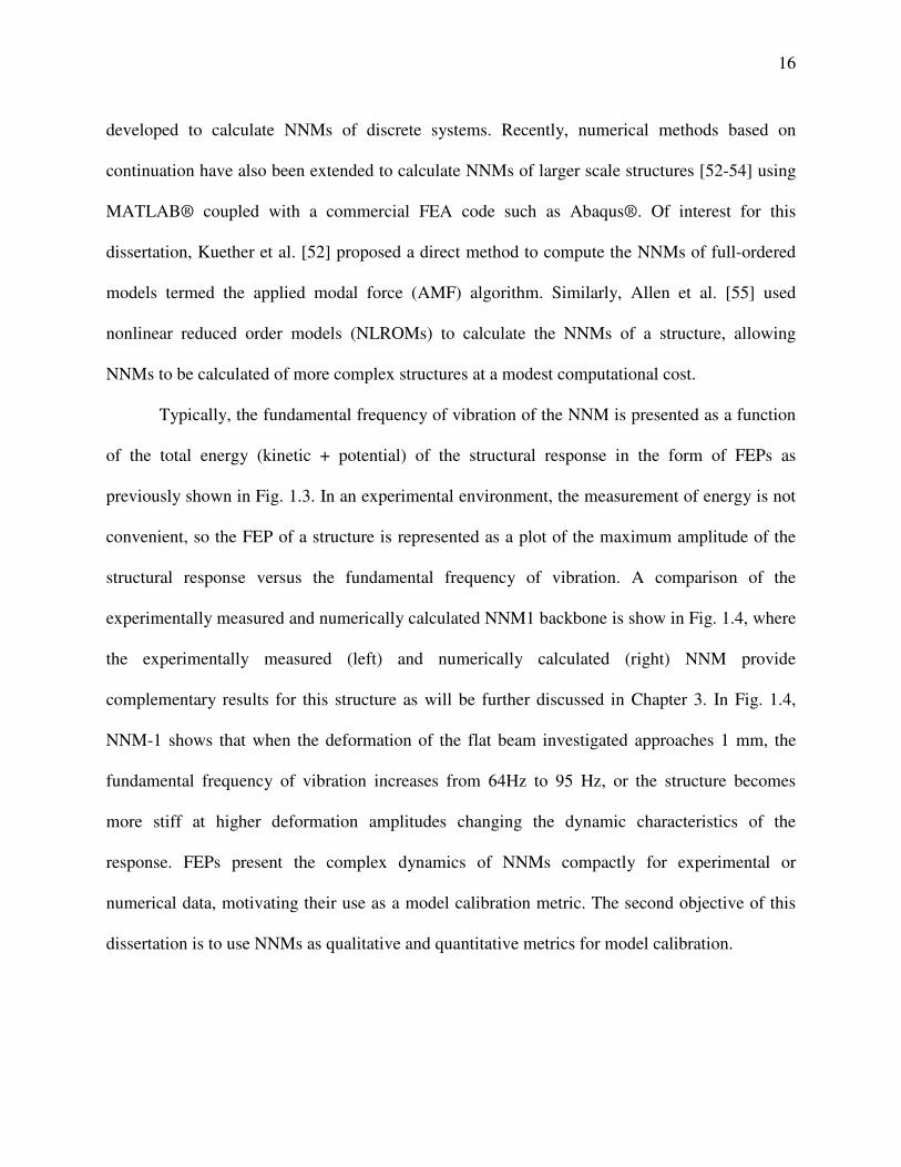
Typically, the fundamental frequency of vibration of the NNM is presented as a function

of the total energy (kinetic + potential) of the structural response in the form of FEPs as

previously shown in Fig. 1.3. In an experimental environment, the measurement of energy is not

convenient, so the FEP of a structure is represented as a plot of the maximum amplitude of the

structural response versus the fundamental frequency of vibration. A comparison of the

experimentally measured and numerically calculated NNM1 backbone is show in Fig. 1.4, where

the experimentally measured (left) and numerically calculated (right) NNM provide

complementary results for this structure as will be further discussed in Chapter 3. In Fig. 1.4,

NNM-1 shows that when the deformation of the flat beam investigated approaches 1 mm, the

fundamental frequency of vibration increases from 64Hz to 95 Hz, or the structure becomes

more stiff at higher deformation amplitudes changing the dynamic characteristics of the

response. FEPs present the complex dynamics of NNMs compactly for experimental or

numerical data, motivating their use as a model calibration metric. The second objective of this

dissertation is to use NNMs as qualitative and quantitative metrics for model calibration.

17

Figure 1.4: Experimental frequency-maximum deformation plot of beam

(Left). Numerical frequency-energy plot of beam (Right).

1.4 Proposed Test and Analysis Methodology

This work proposes the use of continuous-scan laser Doppler vibrometry (CSLDV) and

3-dimensional digital image correlation (3D-DIC) to measure nonlinear normal modes (NNMs)

of geometrically nonlinear structures using manually tuned single point multi-harmonic

excitation where frequency and amplitude of the input force are adjusted to track a NNM. A flow

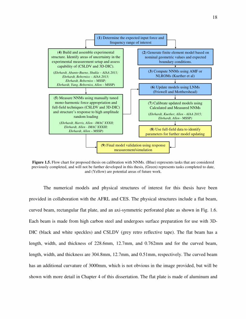
chart describing the model calibration procedure used and the work completed for this

dissertation is shown in Fig. 1.5. LNMs and NNMs were measured and calculated on structures

provided in collaboration with the Air Force Research Lab (AFRL) at Wright Patterson Air

Force Base and Cummins Emissions Solutions (CES) in steps (1-6). Using the resulting LNMs

and NNMs, the models were updated to accurately capture the structural dynamics in linear and

nonlinear response regimes in steps (7-8). Finally, the models are being validated through the use

of linear and nonlinear response measurement and simulation in step (9). The following provides

an in depth discussion of the structures investigated, the tasks completed and avenues of future

work.

60 65 70 75 80 85 90 95 100 10510

-2

10-1

100

Frequency, Hz

Max D

ispla

cem

en

t, m

m

Flat Beam, NNM 1

70 80 90 100 110 120 130 140 150 16010

-7

10-6

10-5

10-4

10-3

10-2

10-1

En

erg

y

Frequency, Hz

Flat Beam, NNM 1

18

(1) Determine the expected input force and

frequency range of interest

(4) Build and assemble experimental

structure. Identify areas of uncertainty in the

experimental measurement setup and assess

capability of (CSLDV and 3D-DIC).

(Ehrhardt, Abanto-Bueno, Shukla – AIAA 2011;

Ehrhardt, Beberniss – AIAA 2013;

Ehrhardt, Beberniss – MSSP;

Ehrhardt, Yang, Beberniss, Allen – MSSP)

(2) Generate finite element model based on

nominal geometric values and expected

boundary conditions.

(5) Measure NNMs using manually tuned

mono-harmonic force appropriation and

full-field techniques (CSLDV and 3D-DIC)

and structure’s response to high amplitude

random loading

(Ehrhardt, Harris, Allen - IMAC XXXII;

Ehrhardt, Allen - IMAC XXXIII;

Ehrhardt, Allen – MSSP)

(3) Compute NNMs using AMF or

NLROMs (Kuether et al)

(7) Calibrate updated models using

Calculated and Measured NNMs

(Ehrhardt, Kuether, Allen - AIAA 2015;

Ehrhardt, Allen - MSSP)

(9) Final model validation using response

measurement/simulation

(8) Use full-field data to identify

parameters for further model updating

(6) Update models using LNMs

(Friswell and Motthershead)

Figure 1.5. Flow chart for proposed thesis on calibration with NNMs. (Blue) represents tasks that are considered

previously completed, and will not be further developed in this thesis, (Green) represents tasks completed to date,

and (Yellow) are potential areas of future work.

The numerical models and physical structures of interest for this thesis have been

provided in collaboration with the AFRL and CES. The physical structures include a flat beam,

curved beam, rectangular flat plate, and an axi-symmetric perforated plate as shown in Fig. 1.6.

Each beam is made from high carbon steel and undergoes surface preparation for use with 3D-

DIC (black and white speckles) and CSLDV (grey retro reflective tape). The flat beam has a

length, width, and thickness of 228.6mm, 12.7mm, and 0.762mm and for the curved beam,

length, width, and thickness are 304.8mm, 12.7mm, and 0.51mm, respectively. The curved beam

has an additional curvature of 3000mm, which is not obvious in the image provided, but will be

shown with more detail in Chapter 4 of this dissertation. The flat plate is made of aluminum and

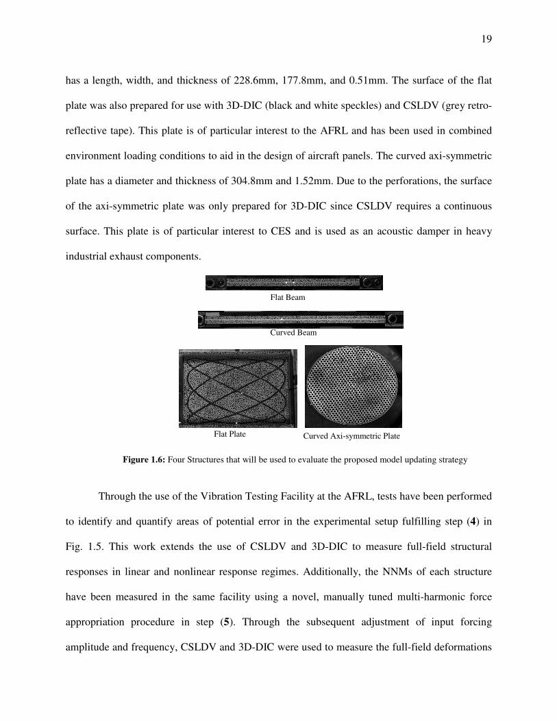
19

has a length, width, and thickness of 228.6mm, 177.8mm, and 0.51mm. The surface of the flat

plate was also prepared for use with 3D-DIC (black and white speckles) and CSLDV (grey retro-

reflective tape). This plate is of particular interest to the AFRL and has been used in combined

environment loading conditions to aid in the design of aircraft panels. The curved axi-symmetric

plate has a diameter and thickness of 304.8mm and 1.52mm. Due to the perforations, the surface

of the axi-symmetric plate was only prepared for 3D-DIC since CSLDV requires a continuous

surface. This plate is of particular interest to CES and is used as an acoustic damper in heavy

industrial exhaust components.

Flat Beam

Flat Plate

Curved Beam

Curved Axi-symmetric Plate

Figure 1.6: Four Structures that will be used to evaluate the proposed model updating strategy

Through the use of the Vibration Testing Facility at the AFRL, tests have been performed

to identify and quantify areas of potential error in the experimental setup fulfilling step (4) in

Fig. 1.5. This work extends the use of CSLDV and 3D-DIC to measure full-field structural

responses in linear and nonlinear response regimes. Additionally, the NNMs of each structure

have been measured in the same facility using a novel, manually tuned multi-harmonic force

appropriation procedure in step (5). Through the subsequent adjustment of input forcing

amplitude and frequency, CSLDV and 3D-DIC were used to measure the full-field deformations

20

along the NNM backbone curve. In collaboration with the AFRL and CES, FEMs based on

nominal geometry and boundary conditions have also been provided in step (2), and through the

use of recently developed methods [52, 56], NNMs have been calculated for each baseline model

in step (3). Using the full-field static measurements taken with 3D-DIC and measured full-field

LNMs of the structures, the initial geometry, boundary conditions, and material properties of

each model have been updated (6). The compact presentation of NNMs in an FEP have been

used to validate the linearly updated models, fulfilling step (7).

For future work, the final steps of the model calibration procedure, step (8), can be

completed by using the measured full-field dynamic data at all harmonics in the response to

identify the nonlinear modal interactions in the structures. A final model validation step can then

be performed using additional measured and simulated response data, completing step (9) and

the model calibration process.

1.5 Scope of the Dissertation

The dissertation is organized as follows. Chapter 2 introduces the CSLDV and 3D-DIC

measurement systems and compares the relative merits of each technique in the measurement of

linear and nonlinear dynamic responses. It is shown that each technique is capable of providing a

dense measurement grid when used to measure the dynamic response of a flat beam and flat

rectangular plate The suitability of CSLDV and 3D-DIC in the nonlinear model updating frame

is also explored here. In Chapter 3, the concept of NNMs is presented in more detail with a

specific focus on their measurement as applied to a flat beam and a curved axi-symmetric plate.

Previous work has detailed the numerical calculation of NNMs, so only a brief summary is

21

presented. Using the experimentally and numerically determined NNMs, a qualitative validation

is performed on a flat beam and a curved beam through updating their boundary conditions and

material properties and is presented in Chapter 4. Chapter 5 provides a summary of the

dissertation and Chapter 6 identifies future work that has been uncovered in the development of

this dissertation.

22

2 The use of Continuous-scan Laser Doppler Vibrometry and 3D Digital

Image Correlation for Full-Field Linear and Nonlinear Measurements

2.1 Introduction

The development of non contact full-field measurement techniques has received

increased attention as the design of high-performance structures has advanced. Due to complex

geometries and the lightweight nature of these structures, there is an increasing need for

experimental techniques capable of measuring the response at a large number of degrees of

freedom without modifying the structural response significantly. Techniques such as

Continuous-Scan Laser Doppler Vibrometry (CSLDV) and high-speed Three-dimensional

Digital Image Correlation (high-speed 3D-DIC) have been developed to meet this need. Both

CSLDV and high-speed 3D-DIC are non-contact, non-destructive, and capable of accurately

measuring the dynamic response at thousands of points across the surface of a structure. Both

techniques are also capable of providing "real-time" measurements, but this has seen limited to

no implementation for several reasons. In the case of 3D-DIC, significant computational power

is needed to move and manipulate the thousands of image files sampled for each test. For

CSLDV, real time measurement is theoretically feasible with the implementation of the

harmonic power spectrum algorithm, but to the best of the authors knowledge this has never been

done. For this work, these limitations are avoided by post-processing the data acquired with both

methods.

2.2 Continuous-scan Laser Doppler Vibrometry

CSLDV is an extension of traditional Laser Doppler Vibrometry (LDV), where the laser

point, instead of dwelling at a fixed location, is continuously moving across a measurement

23

surface. Therefore, obtaining vibration frequencies and deformation shapes from CSLDV signals

is more challenging than from LDV signals since the moving measurement location requires the

system to be treated as time-varying. Though this motion complicates the post-processing, the

benefit provided by the continuously moving point is an increased measurement resolution with

a drastically decreased measurement time when compared with traditional LDV. Several

algorithms have been devised to determine a structure's deformation along the laser scan path.

For example, Ewins et al. treated the operational deflection shape as a polynomial function of the

moving laser position [9, 25-27, 57, 58]. They showed that sideband harmonics appear in the

measured spectrum, each separated by the scan frequency, and that the amplitudes of the

sidebands can be used to determine the polynomial coefficients. Allen et al. later presented a

lifting approach for impulse response measurements [29, 59]. The lifting approach breaks the

CSLDV signal into sets of measurements from each location along the laser path. Hence, the

lifted responses appear to be from a set of pseudo sensors attached to the structure, allowing

conventional modal analysis routines to extract modal parameters from the CSLDV

measurements. However, this method works best when the laser scan frequency is high relative

to the natural frequencies of interest, and for some structures this increase the measurement noise

too much to be practical. Recently, algorithms based on Linear Time Periodic (LTP) system

theory [23, 60-64] were developed and used to derive input-output transfer function and power

spectrum relationships from CSLDV measurements allowing the extraction of a structure's

deformation from impulse, random, and sinusoidal excitations. When a structure is vibrating

sinusoidally, many of the methods simplify significantly and in this paper the simplest method

will be used based on Fourier analysis as was presented by Stanbridge, Martarelli, Ewins and Di

Maio [9, 25-27, 57, 58], and which is called the Fourier series expansion method in [59].

24

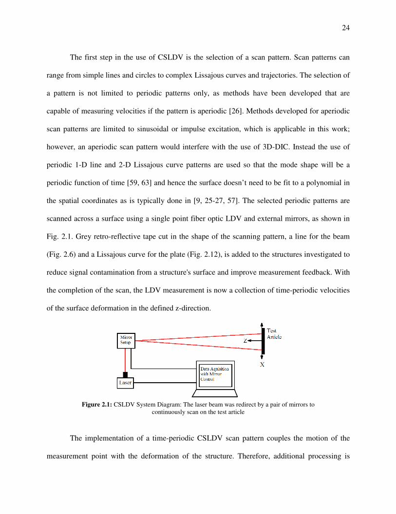
The first step in the use of CSLDV is the selection of a scan pattern. Scan patterns can

range from simple lines and circles to complex Lissajous curves and trajectories. The selection of

a pattern is not limited to periodic patterns only, as methods have been developed that are

capable of measuring velocities if the pattern is aperiodic [26]. Methods developed for aperiodic

scan patterns are limited to sinusoidal or impulse excitation, which is applicable in this work;

however, an aperiodic scan pattern would interfere with the use of 3D-DIC. Instead the use of

periodic 1-D line and 2-D Lissajous curve patterns are used so that the mode shape will be a

periodic function of time [59, 63] and hence the surface doesn’t need to be fit to a polynomial in

the spatial coordinates as is typically done in [9, 25-27, 57]. The selected periodic patterns are

scanned across a surface using a single point fiber optic LDV and external mirrors, as shown in

Fig. 2.1. Grey retro-reflective tape cut in the shape of the scanning pattern, a line for the beam

(Fig. 2.6) and a Lissajous curve for the plate (Fig. 2.12), is added to the structures investigated to

reduce signal contamination from a structure's surface and improve measurement feedback. With

the completion of the scan, the LDV measurement is now a collection of time-periodic velocities

of the surface deformation in the defined z-direction.

Figure 2.1: CSLDV System Diagram: The laser beam was redirect by a pair of mirrors to

continuously scan on the test article

The implementation of a time-periodic CSLDV scan pattern couples the motion of the

measurement point with the deformation of the structure. Therefore, additional processing is

25

required to separate the motion from the structural deformation in order to reconstruct the

vibration shapes. Consider the measurement of vibration along a single axis (the z-axis in this

instance) with a single point sensor. The measured response z(x,y,t) of a linear time invariant

(LTI) structure subjected to a single frequency force input is harmonic at the same frequency, f,

but with a different phase and amplitude at each point, so it can be written as follows.

tfieyxtyx **2),(Re(),,( πZz = (2.1)

Here x and y represent the sensor position on the surface. If CSLDV is used with a

periodic scan pattern, the measured response becomes time periodic, z = z(x(t),y(t),t), as follows

tfietytxttytx **2))(),((Re()),(),(( πZz = (2.2)

where the x- and y-coordinates change in time based on the predefined periodic motion

)2sin()(

)2cos()(

tfAty

tfAtx

yy

xx

π

π

=

= (2.3)

For the Lissajous patterns used here, the period TA of the scan pattern is determined by

both x- and y- scan frequency, as defined in Eqn. (2.4), and modifying the values for fx and fy

changes the density of the pattern across the scan.

=

====

y

y

x

xyyxx

A

Af

Nf

NTNTNf

T1

*1

***1

(2.4)

As the amplitude Z(x(t),y(t)) is periodic, it can be represented with a Fourier Series as

shown below.

( ) ( ) ∑

∞

−∞=

=+==n

tfin

nAAeTtttytx

*2

2

1)()(),(

πZZZZ

(2.5)

26

The periodic motion of the laser couples with the structural deformation inducing a

periodicity in the measurement. Inserting the Fourier series description of the deformation shape

into Eqn. (2.2), one obtains the Fourier description of the CSLDV signal shown in Eqn. (2.6); the

measured response using CSLDV includes motion at the input frequency and an infinite number

of harmonics separated by the scan frequency fA. Since the laser scan path is known, the

deformation of the structure can be recovered by measuring the amplitudes of all of these

harmonics, following a procedure similar to that which was presented in [63].

( ) ( ) ( )∑

∞

−∞=

+==n

tnffi

n

fti Aeetytxttytxππ 22

2

1)(),(),(),( ZZz

(2.6)

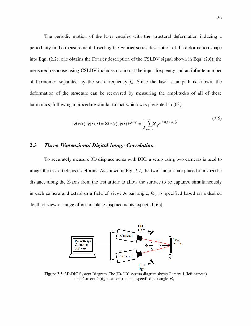
2.3 Three-Dimensional Digital Image Correlation

To accurately measure 3D displacements with DIC, a setup using two cameras is used to

image the test article as it deforms. As shown in Fig. 2.2, the two cameras are placed at a specific

distance along the Z-axis from the test article to allow the surface to be captured simultaneously

in each camera and establish a field of view. A pan angle, Θp, is specified based on a desired

depth of view or range of out-of-plane displacements expected [65].

Figure 2.2: 3D-DIC System Diagram. The 3D-DIC system diagram shows Camera 1 (left camera)

and Camera 2 (right camera) set to a specified pan angle, Θp.

27

Once the stereo camera setup is assembled and fixed, principles of triangulation are used

to establish each camera's position in reference to the global experimental coordinate system as

defined by:

TR +

=

Global

Global

Global

Camera

Camera

Camera

z

y

x

z

y

x (2.7)

Where R is the rotation matrix and T is the translation matrix for the coordinate system

transformation. Additionally, lens distortion and variations between the sensor of the camera and

the final images can be corrected through a bundle adjustment [10]. The coordinate system

transformation matrix is established through the use of images of a rigid known pattern or

calibration panel. With this calibration, the accuracy of the coordinate transformation matrix is

not limited to the pixel size of the imaged surface of the test specimen, but instead can be

interpolated on the sub pixel level (e.g. resolutions of about 0.03 pixels have been obtained [34]).

Once the calibration of the 3D-DIC system is established, images of the fully deformable

structure can be analyzed to obtain displacements. To achieve a sub pixel accuracy in the

determination of displacements, the surface of the structure is divided into areas of pixels or

subsets. Each subset in turn is fit with a surface following the form of:

( )( )

∆

∆

∂∂

∂∂

∂∂

∂∂

+∆∆

∂∂∂

∂∂∂

+

∆

∆

∂∂

∂∂

∂∂

∂∂

+

+

=

2

2

2

2

2

2

2

2

2

2

2

2

y

x

yb

xb

ya

xa

yx

yxb

yxa

y

x

yb

xb

ya

xa

b

a

y

x

B

A

(2.8)

28

Where A and B are the final deformed coordinates of the center of the subset, x and y are

the original coordinates, a and b are the rigid translation of the subset and the three remaining

matrices correspond to an affine, irregular, and quadratic deformation of the subset, respectively.

Using a correlation algorithm, each subset is matched through each imaged deformation

providing out of plane displacement accuracies on the order of 0.03 pixels (or 10 µm for the

field-of-view used in this work) depending on the correlation algorithm used. In-plane

deformations are measured with a greater accuracy when compared with purely out-of-plane

deformations since these deformation are less reliant on the higher order fit. Prior to testing, a

high-contrast random gray-scale pattern is applied to the measurement surface so the defined

subsets can be uniquely and accurately fit. As detailed in [10], triangulation of the subset

matching is used to determine the coordinate value of each measurement point.

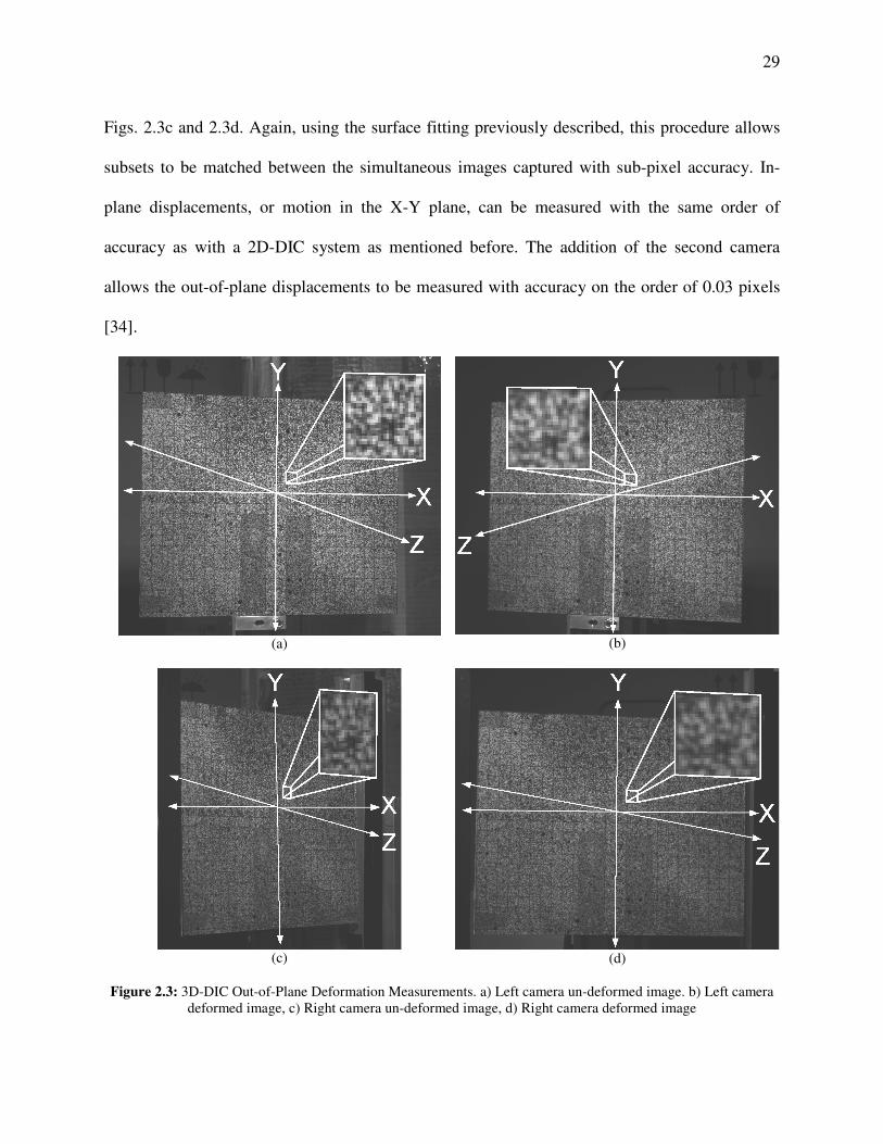
An example of the measurement of a out of plane rotation is shown in Fig. 2.3. During

characterization of the 3D-DIC system a measuring coordinate system as shown in Figs. 2.3a and

2.3b is established. Images are captured throughout deformation as shown in Figs. 2.3c and 2.3d.

Using the image captured in the un-deformed condition for Camera 1 (Fig. 2.3a), subsets of the

image are established. Subset matching is performed between the un-deformed condition for

Camera 1 and the un-deformed condition for Camera 2 (Fig. 2.3b). As the test article experiences

deformation, images are captured with each camera simultaneously. Subset matching is then

performed between the un-deformed image of Camera 1 (Fig. 2.3a) and the deformed image of

Camera 1 (Fig. 2.3c). Once the subsets have been established in the deformed image of Camera 1

(Fig. 2.3c), a second stage of subset matching is performed between the deformed image of

Camera 1 (Fig. 2.3c) and the deformed image of Camera 2 (Fig. 2.3d). An out-of-plane rigid

body rotation about the Y-axis of the un-deformed test article (Figs 2.3a and 2.3b) is shown in

29

Figs. 2.3c and 2.3d. Again, using the surface fitting previously described, this procedure allows

subsets to be matched between the simultaneous images captured with sub-pixel accuracy. In-

plane displacements, or motion in the X-Y plane, can be measured with the same order of

accuracy as with a 2D-DIC system as mentioned before. The addition of the second camera

allows the out-of-plane displacements to be measured with accuracy on the order of 0.03 pixels

[34].

(a)

(b)

(c)

(d)

Figure 2.3: 3D-DIC Out-of-Plane Deformation Measurements. a) Left camera un-deformed image. b) Left camera

deformed image, c) Right camera un-deformed image, d) Right camera deformed image

30

One difficulty in a 3D-DIC setup is establishing uniform lighting over large out-of-plane

deformations experienced by the test article. Since uniform lighting is hard to establish, accuracy

in out-of-plane measurements vary with Z distance from the test article. Also, to establish the 3D

measuring coordinate system, a system characterization that is more involved than the 2D case is

needed. Typically 10-20 images of a plate with a known pattern is subjected to a rigid-body

displacement in the desired measuring volume to create the 3D measuring coordinate system.

2.4 Experimental Setup

The physical experimental setup is shown in Fig. 2.4. In this setup, there are four main

systems: 1) exciter/ controller, 2) static 3D-DIC system, 3) dynamic 3D-DIC system, and 4) the

CSLDV system.

1) Excitation was provided by two separate exciters, both controlled in an open-loop

using a Wavetek Variable Phase Synthesizer. The low amplitude excitation was provided by an

Electro Corporation 2030 PHT magnetic pickup which was given a high voltage input from a

Piezo Amplifier. This induces a localized magnetic field providing a near single point input force

to ferrous materials. If non-ferrous materials are used or more force is required, a thin magnetic

metal dot can be added to a structure. The force exerted by the magnetic pickup was measured

using a force transducer mounted to a solid base between a solid base and the magnetic pickup

providing measurement of the reaction force with the base. Large amplitude excitation was

provided by shaking the base of the structure's clamping fixture which was mounted on a 5000N

MB dynamics shaker. However, this type of excitation provides symmetric inertial loading at a

constant acceleration and limits the ability to examine asymmetric motion of the structure. The

voltage input to the exciter was measured as well as the input force for the magnetic driver and

the base acceleration for the shaker. The velocity response and input voltage signals were

31

analyzed in real time using a Onosoki FFT Analyzer to track the phase between the signals.

Here, the input voltage was used instead of the measured force/acceleration to limit noise

contamination from the measurement sensors. However, the measured force/acceleration signals

were compared after measurement to ensure the correct phase relationship between input and

response was maintained. The structure's fundamental frequencies in linear and nonlinear

response regimes could then be determined by adjusting the frequency until the input voltage and

response velocity are 180 degrees out of phase.

2) The static 3D-DIC system consists of two Prosilica GT2750 CCD cameras with a full

resolution of 2750 x 2200 pixels with a maximum frame rate of 20 fps. For this experimental

setup, full resolution images were used since the amount of available memory in the cameras was

not limited and to include the greatest amount of pixels in the measurement . The static system

uses 18mm lenses and is positioned at a standoff distance of 580mm with a camera angle of 26

degrees. All static displacements were determined using a commercial 3D-DIC software Aramis

using subsets of 31x31 pixels with a 13 pixel overlap across the entire surface of the plate. A

250mm x 200mm calibration panel was used to establish the measurement volume and lead to a

calibration deviation of 0.032 pixels for this camera resolution or 0.004 mm for this field of

view.

3) The dynamic 3D-DIC system includes two Photron, high speed 12-bit CMOS cameras

(model Fastcam SA5 775K-M3K). Each camera has 32GB of memory onboard with a maximum

resolution of 1024×1024 pixels. For each experimental setup, image size was adjusted to fit as

much of the structure in the frame of both cameras. The dynamic system uses 85mm lenses at a

stand off distance of 1370mm with a camera angle of 24.4 degrees. All dynamic displacements

were determined using a software extension of Aramis called IVIEW Real Time Sensor [66]

32

using subsets of 15x15 pixels. In order to minimize the heat generated and remove the electrical

noise produced by the lighting systems that are typically used in high-speed DIC systems, two

305×305 LED light panels were used. The cameras and the data acquisition system were

simultaneously started using an external TTL trigger. Measurement points were selected to avoid

the retro-reflective tape, so there is no overlap of measurements between CSLDV and 3D-DIC.

This was done to reduce the measurement noise previously seen in the static measurements and

provide better tracking for the DIC algorithm. A 250mm x 200mm calibration panel was used to

establish the measurement volume and lead to a calibration deviation of 0.02 pixels for this

camera resolution or 0.007 mm for this field of view.

4) The continuous-scan mechanism was built using a Polytec OFV-552 fiber optic laser

vibrometer with a sensitivity of 125 mm/s/V and the same external mirror system that was used

in [29]. The mirrors were positioned at a stand off distance of 2.4m, which was selected to

minimize the scan angle, which was a maximum of 7.3 degrees in x-direction and 5.4 degrees in

y-direction for both setups, and yet keep the laser close enough to maintain a high quality signal.

The external mirror system consisted of two galvanometer scanners in open-loop control; each

scanner had a position detector that measured the instantaneous rotation angle, allowing precise

and accurate control and measurement of the laser position. The control and data acquisition

system was built using a National Instruments PXI system. A LabVIEW program was developed

to integrate several features including the function generator, data acquisition, and signal

processing. The line and Lissajous patterns used for this investigation have a x-direction scan

frequency of 3 Hz and the y-direction scan frequency is 4 Hz. Data was collected at each steady

state response level with a sampling frequency of 10,240Hz for 2 minutes.

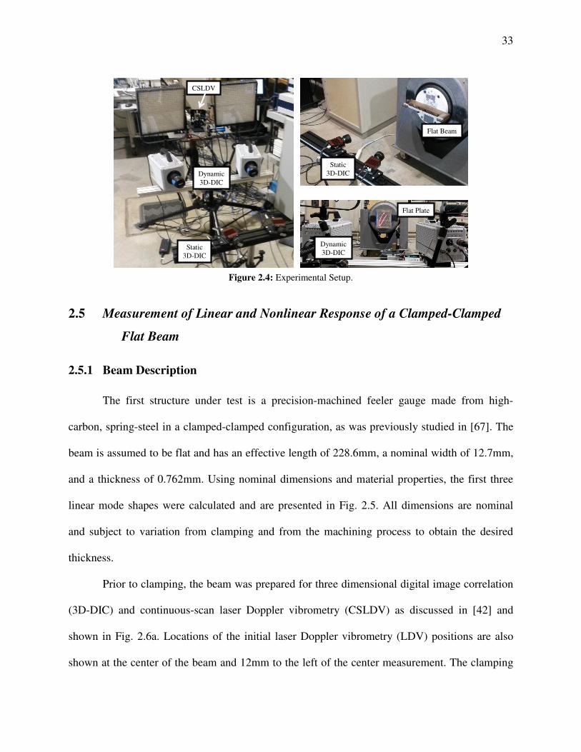
33

Static

3D-DIC

Dynamic

3D-DIC

CSLDV

Static

3D-DIC

Flat Beam

Flat Plate

Dynamic

3D-DIC

Figure 2.4: Experimental Setup.

2.5 Measurement of Linear and Nonlinear Response of a Clamped-Clamped

Flat Beam

2.5.1 Beam Description

The first structure under test is a precision-machined feeler gauge made from high-

carbon, spring-steel in a clamped-clamped configuration, as was previously studied in [67]. The

beam is assumed to be flat and has an effective length of 228.6mm, a nominal width of 12.7mm,

and a thickness of 0.762mm. Using nominal dimensions and material properties, the first three

linear mode shapes were calculated and are presented in Fig. 2.5. All dimensions are nominal

and subject to variation from clamping and from the machining process to obtain the desired

thickness.

Prior to clamping, the beam was prepared for three dimensional digital image correlation

(3D-DIC) and continuous-scan laser Doppler vibrometry (CSLDV) as discussed in [42] and

shown in Fig. 2.6a. Locations of the initial laser Doppler vibrometry (LDV) positions are also

shown at the center of the beam and 12mm to the left of the center measurement. The clamping

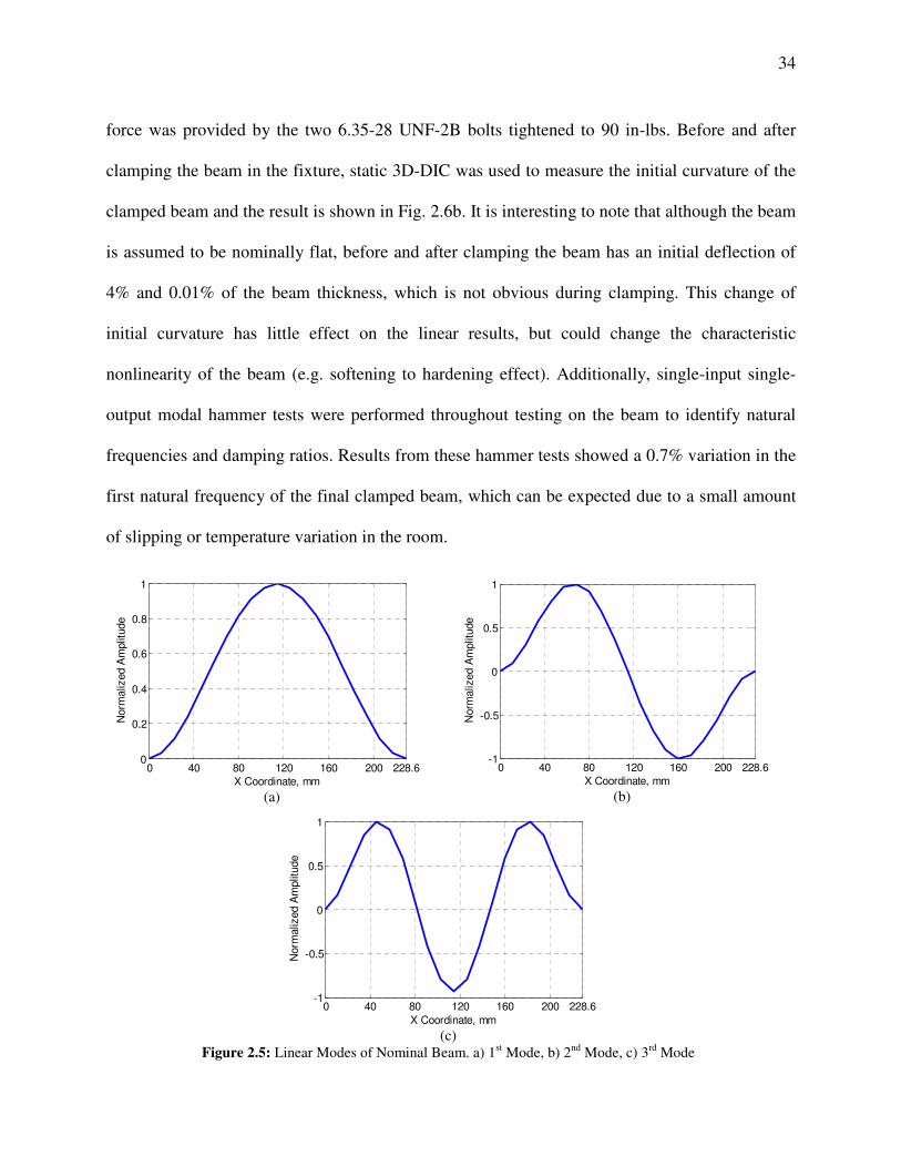
34

force was provided by the two 6.35-28 UNF-2B bolts tightened to 90 in-lbs. Before and after

clamping the beam in the fixture, static 3D-DIC was used to measure the initial curvature of the

clamped beam and the result is shown in Fig. 2.6b. It is interesting to note that although the beam

is assumed to be nominally flat, before and after clamping the beam has an initial deflection of

4% and 0.01% of the beam thickness, which is not obvious during clamping. This change of

initial curvature has little effect on the linear results, but could change the characteristic

nonlinearity of the beam (e.g. softening to hardening effect). Additionally, single-input single-

output modal hammer tests were performed throughout testing on the beam to identify natural

frequencies and damping ratios. Results from these hammer tests showed a 0.7% variation in the

first natural frequency of the final clamped beam, which can be expected due to a small amount

of slipping or temperature variation in the room.

0 40 80 120 160 200 228.60

0.2

0.4

0.6

0.8

1

Norm

aliz

ed A

mplit

ude

X Coordinate, mm (a)

0 40 80 120 160 200 228.6-1

-0.5

0

0.5

1

X Coordinate, mm

Norm

aliz

ed A

mplit

ude

(b)

0 40 80 120 160 200 228.6-1

-0.5

0

0.5

1

X Coordinate, mm

Norm

aliz

ed A

mplit

ude

(c)

Figure 2.5: Linear Modes of Nominal Beam. a) 1st Mode, b) 2

nd Mode, c) 3

rd Mode

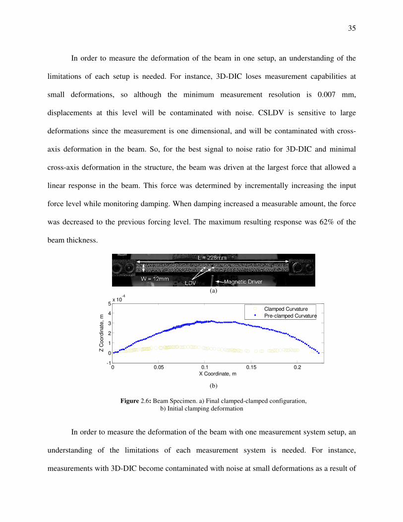
35

In order to measure the deformation of the beam in one setup, an understanding of the

limitations of each setup is needed. For instance, 3D-DIC loses measurement capabilities at

small deformations, so although the minimum measurement resolution is 0.007 mm,

displacements at this level will be contaminated with noise. CSLDV is sensitive to large

deformations since the measurement is one dimensional, and will be contaminated with cross-

axis deformation in the beam. So, for the best signal to noise ratio for 3D-DIC and minimal

cross-axis deformation in the structure, the beam was driven at the largest force that allowed a

linear response in the beam. This force was determined by incrementally increasing the input

force level while monitoring damping. When damping increased a measurable amount, the force

was decreased to the previous forcing level. The maximum resulting response was 62% of the

beam thickness.

(a)

0 0.05 0.1 0.15 0.2-1

0

1

2

3

4

5x 10

-4

X Coordinate, m

Z C

oord

inate

, m

Clamped Curvature

Pre-clamped Curvature

(b)

Figure 2.6: Beam Specimen. a) Final clamped-clamped configuration,

b) Initial clamping deformation

In order to measure the deformation of the beam with one measurement system setup, an

understanding of the limitations of each measurement system is needed. For instance,

measurements with 3D-DIC become contaminated with noise at small deformations as a result of

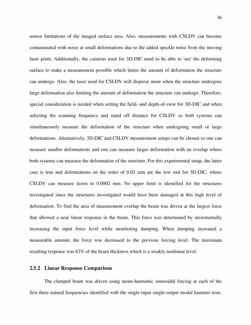
36

sensor limitations of the imaged surface area. Also, measurements with CSLDV can become

contaminated with noise at small deformations due to the added speckle noise from the moving

laser point. Additionally, the cameras used for 3D-DIC need to be able to 'see' the deforming

surface to make a measurement possible which limits the amount of deformation the structure

can undergo. Also, the laser used for CSLDV will disperse more when the structure undergoes

large deformation also limiting the amount of deformation the structure can undergo. Therefore,

special consideration is needed when setting the field- and depth-of-view for 3D-DIC and when

selecting the scanning frequency and stand off distance for CSLDV so both systems can

simultaneously measure the deformation of the structure when undergoing small or large

deformations. Alternatively, 3D-DIC and CSLDV measurement setups can be chosen so one can

measure smaller deformations and one can measure larger deformation with an overlap where

both systems can measure the deformation of the structure. For this experimental setup, the latter

case is true and deformations on the order of 0.02 mm are the low end for 3D-DIC, where

CSLDV can measure down to 0.0002 mm. No upper limit is identified for the structures

investigated since the structures investigated would have been damaged at this high level of

deformation. To find the area of measurement overlap the beam was driven at the largest force

that allowed a near linear response in the beam. This force was determined by incrementally

increasing the input force level while monitoring damping. When damping increased a

measurable amount, the force was decreased to the previous forcing level. The maximum

resulting response was 62% of the beam thickness which is a weakly nonlinear level.

2.5.2 Linear Response Comparison

The clamped beam was driven using mono-harmonic sinusoidal forcing at each of the

first three natural frequencies identified with the single-input single-output modal hammer tests.

37

The beam's steady state response under these forcing conditions was measured using high-speed

3D-DIC and CSLDV. Fig. 2.7(a) shows an example of the response spectrum from 3D-DIC

measured at the center of the beam when it is forced at the first natural frequency. Only the out-

of-plane displacements are shown for 3D-DIC since the axial and transverse displacements are in

the noise of the measurement. As expected, a single harmonic is seen in the response at 71.3Hz,

which is the forcing frequency. Fig. 2.7 (b) shows an example of the response spectrum from

CSLDV measured as the laser scans the beam's surface. In addition to the primary harmonic of

the response at 71.3Hz, several side-bands are observed in the response spectrum each separated

by the scanning frequency of 3Hz. As previously discussed, an infinite number of sidebands are

expected for CSLDV, but Fig. 2.7(b) shows sideband harmonics higher than the 6th order are

buried in the noise floor. So, no harmonics above the 6th order were used when construction the

mode shape. The Fourier coefficients for harmonics of n = -6:6 were then used to construct the

mode shape along the laser path. The second and third bending mode shapes were reconstructed

using the Fourier coefficients that stood out about the noise floor, which ended up being

harmonics n=-10...10 and n=-15...15.

0 20 40 60 8010

-4

10-2

100

102

Frequency, Hz

Mag P

SD

0 20 40 60 8010

-2

100

102

104

Frequency, Hz

Mag P

SD

-7

-6

-5

-4 -3

-2 -1

0

1

2

3

4

5

6

7

fA = 3Hz

Figure 2.7: Linear Response Spectrum Comparison. 3D-DIC (Left) and CSLDV (Right)

38

Figure 2.8 compares the mode shapes obtained by CSLDV and 3D-DIC when exciting

near each of the three resonance frequencies. Figure 2.8a contains the mode shape at 71.3Hz and

shows the difference between the mode shapes measured with CSLDV and the measurement

points obtained with high-speed 3D-DIC. Similarly, Fig. 2.8b and 2.8c show the mode shapes at

205.5Hz and 411.4Hz. The MAC values between DIC and the CSLDV shapes are shown in Tab.

2.1 along with the frequency errors previously discussed. It is noted that MAC values for modes

1 and 2 are above 0.99 showing excellent correlation between CSLDV and high-speed 3D-DIC;

for the third mode at 411 Hz the maximum displacement was only 0.21mm measured at

411.4Hz, high-speed 3D-DIC begins to exhibit larger errors in the mode shape, which is shown

in Fig. 2.8c, leading to a MAC value of 0.6572.

0 30 60 90 120 150 180 210 228.60

0.2

0.4

0.6

0.8

1

X Coordinate, mm

Norm

aliz

ed A

mplit

ude

CSLDV

3D-DIC

(a)

0 30 60 90 120 150 180 210 228.6-1

-0.5

0

0.5

1

X Coordinate, mm

Norm

aliz

ed A

mplit

ude

CSLDV

3D-DIC

(b)

0 30 60 90 120 150 180 210 228.6

-1

-0.5

0

0.5

1

X Coordinate, mm

Norm

aliz

ed A

mplit

ude

CSLDV

3D-DIC

(c)

Figure 2.8: Modes shapes from Steady State Excitation. a) Mode 1 at 71.3Hz, b) Mode 2 at 204.5Hz, and c) Mode 3 at

411.4Hz.

39

Table 2.1: Modal Comparison

Mode

fn AVG

Modal

Hammer

Test, Hz

% Change

between Pre- and

Post- Experiment

Modal Hammer

Tests

fn CSLDV,

Hz

% Error

CSLDV fn DIC, Hz % Error DIC MAC

1 71.75 -0.70 71.24 -0.7112 71.30 -0.6269 0.9995

2 204.35 -0.49 204.33 -0.0117 204.50 0.0747 0.9981 Sinusoidal

3 411.45 -0.12 411.05 -0.0972 411.39 -0.0134 0.6572

Additionally an asymmetry is seen in the mode shapes of modes 2 and 3 which is

believed a result of asymmetry of the boundary conditions or the initial curvature in the beam.

Both measurement methods capture the asymmetry in mode 2, but the asymmetry for mode 3 is

apparently not detected as accurately in CSLDV as with 3D-DIC. The accuracy of each method

is difficult to ascertain for the measurement of mode 3 since 3D-DIC begins to lose measurement

resolution and higher harmonics from CSLDV measurements are buried in the noise of the laser

signal. In either case, the asymmetry would be undetectable unless the dynamic response is

observed with the large number of measurement points.

It is also important to note that while the smooth nature of the CSLDV mode shapes

seems to suggest that they are infallible, they are in fact an approximation of the true mode

shapes obtained by expanding them in a Fourier series of the time-varying scan pattern. The

accuracy of the reconstructed mode shape depends on the number of harmonics included in the

Fourier series approximation. As mentioned previously, thirteen clearly dominant harmonics (i.e.

n=-6...6) were observed for the first mode. The neglected harmonics were at least a few orders of

magnitude smaller than the dominant ones, so one would be inclined to have high confidence in

that shape. The harmonics n = -8...8 were also used to reconstruct the first bending mode shape,

40

the results was only 0.068% different from the shape that was shown which used harmonics n = -

6...6. Furthermore, because the laser is scanning along a line with CSLDV, when the

measurements are noisy, the mode shapes measured on the forward and backward parts of the

sweep tend to differ giving an indication of the error. Here, the forward and backward sweeps

overlay completely suggesting that the shapes shown are quite accurate.

2.5.3 Nonlinear Response Comparison

As a structure is pushed towards the nonlinear regime, a single harmonic input force

results in a multi-harmonic response. Figure 2.9 shows the resulting nonlinear response spectrum

for 3D-DIC and CSLDV. For 3D-DIC, 10 harmonics of the forcing frequency can be easily

identified in the measured response. The additional harmonics seen in the 3D-DIC response near

140 Hz can be attributed to previously identified fan noise from the camera cooling fans. As

discussed later, the deformation shape at all 10 harmonics cannot be fully visualized for 3D-DIC

due to variations in the measurement across the surface, especially when the response has small

displacement. For CSLDV, the scanning laser permits the identification of 7 harmonics of the

forcing frequency in the measured response. Due to increased laser dispersion from the 3Hz

motion of the laser the noise floor is increased reducing the ability to identify all 10 of the

fundamental harmonic components. Also, at higher harmonics, the deformation shape of the

beam becomes more complex, so more side band harmonics are needed to reconstruct the

deformation shape of the beam. However, the added noise of the scanning laser reduces the

ability to identify side band harmonics in the measured response.

41

0 100 200 300 400 500 600 700 800 900 100010

-1

100

101

102

103

104

Frequency, Hz

Ma

g P

SD

100 200 300 400 500 600 700 800 900 1000

100

101

102

103

104

105

Frequency (Hz)

Ma

g P

SD

Figure 2.9: Nonlinear Beam Response Spectrum Comparison. (Left) 3D-DIC and (Right) CSLDV

Full-field measurements of a deforming structure, such as this beam, are especially

beneficial for nonlinear deformations since the spatial deformation of the beam can be identified

at each harmonic. These measurements can then in turn be used in model updating to identify

nonlinear coupling in the beam's modes. Fig. 2.10a-e shows the deformation patterns along the

beam for selected harmonics. Fig. 2.10a shows the first harmonic of the response, or the

fundamental harmonic, which resembles the first linear mode of a flat beam as expected. There is

a small shift in the deformation of the first harmonic made with CSLDV and 3D-DIC, but both

systems correctly show a zero deformation at the clamps of the beam. Each measurement system

establishes an independent reference coordinate system, and this shift corresponds to a 6 degree

rotation about the y-axis of one of the measurement systems relative to the other. This is

certainly within the uncertainty in the alignment of the two measurement systems. Fig. 2.10b

shows the second harmonic of the response, which resembles the second linear mode of a flat

beam, with a factor of two difference between the peak deformation of each lobe. The maximum

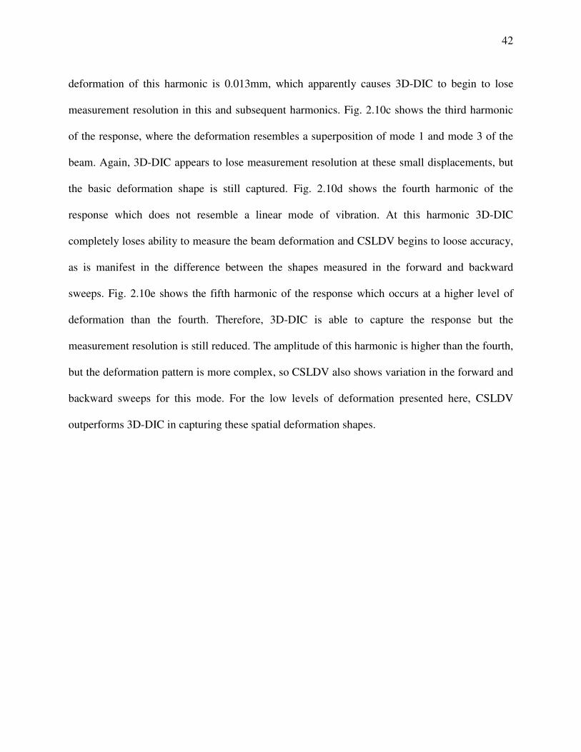
42

deformation of this harmonic is 0.013mm, which apparently causes 3D-DIC to begin to lose

measurement resolution in this and subsequent harmonics. Fig. 2.10c shows the third harmonic

of the response, where the deformation resembles a superposition of mode 1 and mode 3 of the

beam. Again, 3D-DIC appears to lose measurement resolution at these small displacements, but

the basic deformation shape is still captured. Fig. 2.10d shows the fourth harmonic of the

response which does not resemble a linear mode of vibration. At this harmonic 3D-DIC

completely loses ability to measure the beam deformation and CSLDV begins to loose accuracy,

as is manifest in the difference between the shapes measured in the forward and backward

sweeps. Fig. 2.10e shows the fifth harmonic of the response which occurs at a higher level of

deformation than the fourth. Therefore, 3D-DIC is able to capture the response but the

measurement resolution is still reduced. The amplitude of this harmonic is higher than the fourth,

but the deformation pattern is more complex, so CSLDV also shows variation in the forward and

backward sweeps for this mode. For the low levels of deformation presented here, CSLDV

outperforms 3D-DIC in capturing these spatial deformation shapes.

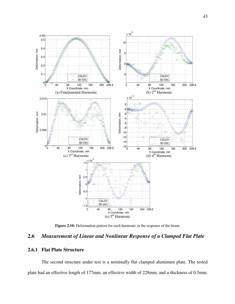
43

0 40 80 120 160 200 228.60

0.1

0.2

0.3

0.4

0.5

0.55

X Coordinate, mm

Defo

rmation,

mm

CSLDV

3D-DIC

(a) Fundamental Harmonic

0 40 80 120 160 200 228.6

-5

0

5

10

x 10-3

X Coordinate, mm

Defo

rmation,

mm

CSLDV

3D-DIC

(b) 2

nd Harmonic

0 40 80 120 160 200 228.60

0.005

0.01

0.015

X Coordinate, mm

Defo

rmation,

mm

CSLDV

3D-DIC

(c) 3

rd Harmonic

0 40 80 120 160 200 228.6-16

-14

-12

-10

-8

-6

-4

-2

0

2

x 10-4

X Coordinate, mm

Defo

rmation,

mm

CSLDV

3D-DIC

(d) 4

th Harmonic

0 40 80 120 160 200 228.6

-1.5

-1

-0.5

0

0.5

1

1.5x 10

-3

X Coordinate, mm

Defo

rmation,

mm

CSLDV

3D-DIC

(e) 5

th Harmonic

Figure 2.10: Deformation pattern for each harmonic in the response of the beam.

2.6 Measurement of Linear and Nonlinear Response of a Clamped Flat Plate

2.6.1 Flat Plate Structure

The second structure under test is a nominally flat clamped aluminum plate. The tested

plate had an effective length of 177mm, an effective width of 228mm, and a thickness of 0.5mm.

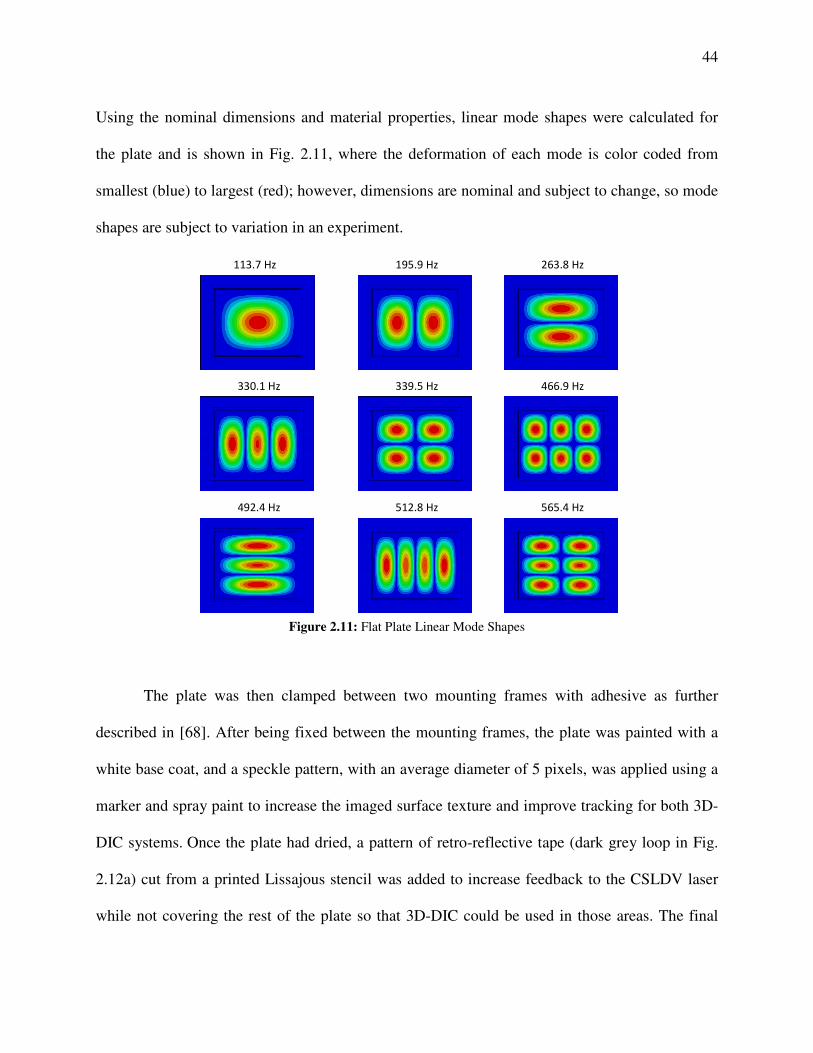
44

Using the nominal dimensions and material properties, linear mode shapes were calculated for

the plate and is shown in Fig. 2.11, where the deformation of each mode is color coded from

smallest (blue) to largest (red); however, dimensions are nominal and subject to change, so mode

shapes are subject to variation in an experiment.

113.7 Hz 195.9 Hz 263.8 Hz

330.1 Hz 339.5 Hz 466.9 Hz

492.4 Hz 512.8 Hz 565.4 Hz

Figure 2.11: Flat Plate Linear Mode Shapes

The plate was then clamped between two mounting frames with adhesive as further

described in [68]. After being fixed between the mounting frames, the plate was painted with a

white base coat, and a speckle pattern, with an average diameter of 5 pixels, was applied using a

marker and spray paint to increase the imaged surface texture and improve tracking for both 3D-

DIC systems. Once the plate had dried, a pattern of retro-reflective tape (dark grey loop in Fig.

2.12a) cut from a printed Lissajous stencil was added to increase feedback to the CSLDV laser

while not covering the rest of the plate so that 3D-DIC could be used in those areas. The final

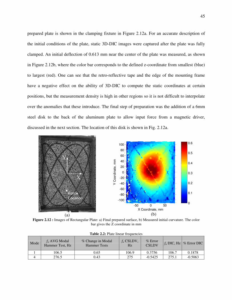
45

prepared plate is shown in the clamping fixture in Figure 2.12a. For an accurate description of

the initial conditions of the plate, static 3D-DIC images were captured after the plate was fully

clamped. An initial deflection of 0.613 mm near the center of the plate was measured, as shown

in Figure 2.12b, where the color bar corresponds to the defined z-coordinate from smallest (blue)

to largest (red). One can see that the retro-reflective tape and the edge of the mounting frame

have a negative effect on the ability of 3D-DIC to compute the static coordinates at certain

positions, but the measurement density is high in other regions so it is not difficult to interpolate

over the anomalies that these introduce. The final step of preparation was the addition of a 6mm

steel disk to the back of the aluminum plate to allow input force from a magnetic driver,

discussed in the next section. The location of this disk is shown in Fig. 2.12a.

(a)

-50 0 50

-100

-80

-60

-40

-20

0

20

40

60

80

100

X Coordinate, mm

Y C

oord

inate

, m

m

0

0.1

0.2

0.3

0.4

0.5

0.6

(b)

Figure 2.12 : Images of Rectangular Plate: a) Final prepared surface, b) Measured initial curvature. The color

bar gives the Z coordinate in mm

Table 2.2: Plate linear frequencies

Mode fn AVG Modal

Hammer Test, Hz

% Change in Modal

Hammer Tests

fn CSLDV,

Hz

% Error

CSLDV fn DIC, Hz % Error DIC

1 106.5 0.65 106.9 0.3756 106.7 0.1878

4 276.5 0.43 275 -0.5425 275.1 -0.5063

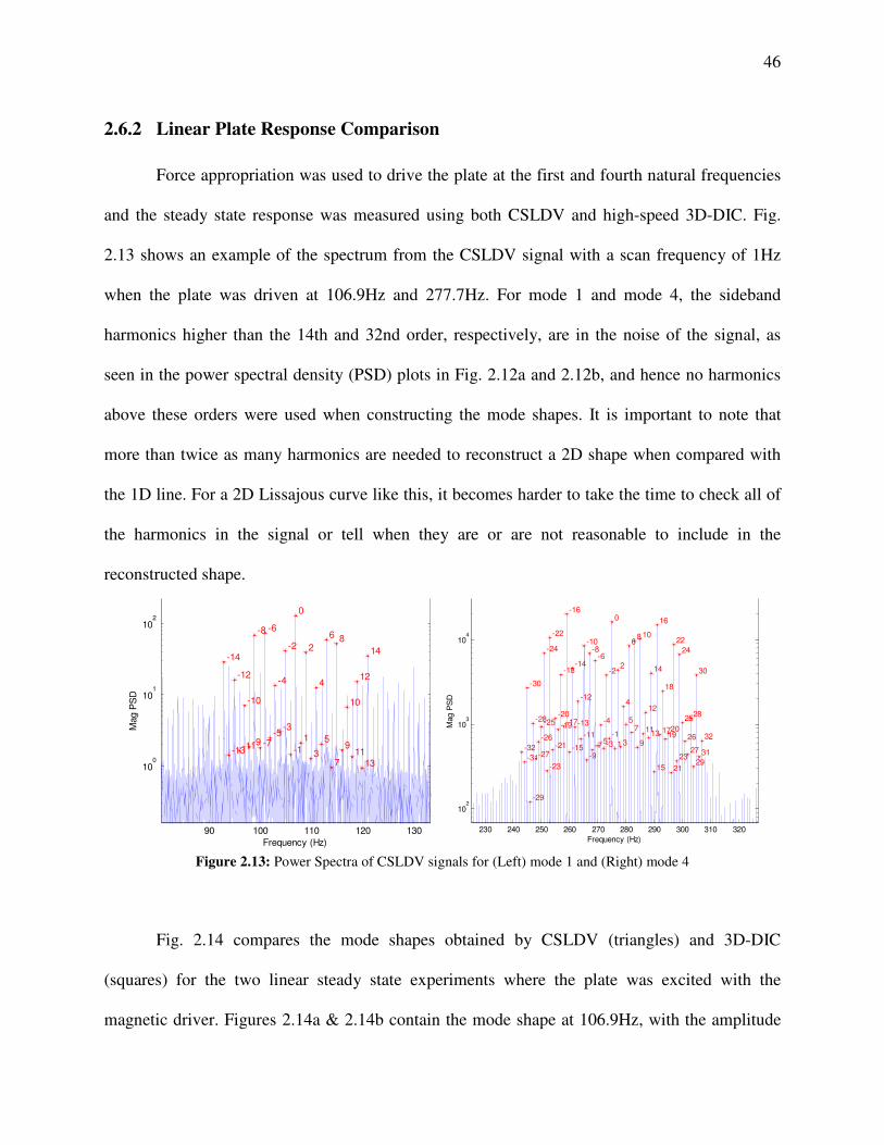
46

2.6.2 Linear Plate Response Comparison

Force appropriation was used to drive the plate at the first and fourth natural frequencies

and the steady state response was measured using both CSLDV and high-speed 3D-DIC. Fig.

2.13 shows an example of the spectrum from the CSLDV signal with a scan frequency of 1Hz

when the plate was driven at 106.9Hz and 277.7Hz. For mode 1 and mode 4, the sideband

harmonics higher than the 14th and 32nd order, respectively, are in the noise of the signal, as

seen in the power spectral density (PSD) plots in Fig. 2.12a and 2.12b, and hence no harmonics

above these orders were used when constructing the mode shapes. It is important to note that

more than twice as many harmonics are needed to reconstruct a 2D shape when compared with

the 1D line. For a 2D Lissajous curve like this, it becomes harder to take the time to check all of

the harmonics in the signal or tell when they are or are not reasonable to include in the

reconstructed shape.

90 100 110 120 130

100

101

102

Frequency (Hz)

Mag P

SD

-14

-13

-12

-11

-10

-9

-8

-7

-6

-5

-4

-3

-2

-1

0

1

2

3

4

5

6

7

8

9

10

11

12

13

14

230 240 250 260 270 280 290 300 310 320

102

103

104

Frequency (Hz)

Mag P

SD

-32 -31

-30

-29

-28

-27

-26

-25

-24

-23

-22

-21

-20 -19

-18

-17

-16

-15

-14

-13

-12

-11

-10

-9

-8

-7

-6

-5

-4

-3

-2

-1

0

1

2

3

4 5

6

7

8

9

10

11

12

13

14

15

16

17

18

19

20

21

22

23

24

25

26 27

28

29

30

31

32

Figure 2.13: Power Spectra of CSLDV signals for (Left) mode 1 and (Right) mode 4

Fig. 2.14 compares the mode shapes obtained by CSLDV (triangles) and 3D-DIC

(squares) for the two linear steady state experiments where the plate was excited with the

magnetic driver. Figures 2.14a & 2.14b contain the mode shape at 106.9Hz, with the amplitude

47

color coded from low (blue) to high (red) amplitude. Although the defined measurement grids

for CSLDV and 3D-DIC don't overlap, both measurements show good agreement between both

techniques. Since there are no directly overlapping measurement points, MAC values cannot be

calculated to compare the measured shapes, so only a qualitative comparison is made. The focus

of this work was on modes of a rectangular plate that would be excited with the use of symmetric

loading (i.e. in the application of interest the aircraft panels are excited by uniform pressure

loads), so the next linear mode examined was mode 4. Since mode 4, is symmetric it can be

excited with base excitation from the larger shaker. Figures 2.14c & 2.14d contain the mode

shape at 277.70 Hz and again show good agreement between measurements.

-0.05 0 0.05

-0.1

-0.05

0

0.05

0.1

X Coordinate, m

Y C

oord

inate

, m

CSLDV

3D-DIC

(a)

-0.05 0 0.050

0.1

0.2

0.3

0.4

0.5

0.6

0.7

0.8

0.9

1

X Coordinate, m

Norm

aliz

ed A

mplit

ude

CSLDV

3D-DIC

(b)

-0.05 0 0.05

-0.1

-0.05

0

0.05

0.1

X Coordinate, m

Y C

oord

inate

, m

CSLDV

3D-DIC

(c)

-0.1 -0.05 0 0.05 0.1-1

-0.8

-0.6

-0.4

-0.2

0

0.2

0.4

0.6

0.8

1

Y Coordinate, m

Norm

alized A

mp

litu

de

CSLDV

3D-DIC

(d)

Figure 2.14: Mode Shape Comparison between CSLDV and 3D-DIC. a) & b) Mode 1, c) & d) Mode 4

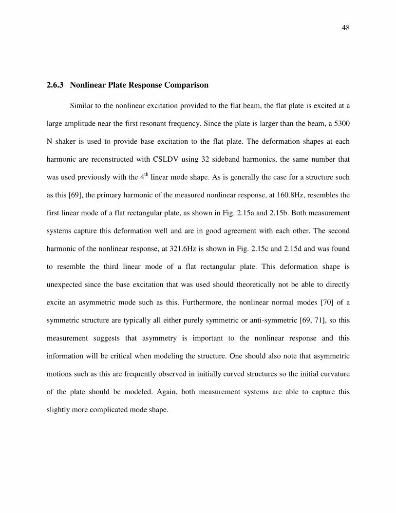
48

2.6.3 Nonlinear Plate Response Comparison

Similar to the nonlinear excitation provided to the flat beam, the flat plate is excited at a

large amplitude near the first resonant frequency. Since the plate is larger than the beam, a 5300

N shaker is used to provide base excitation to the flat plate. The deformation shapes at each

harmonic are reconstructed with CSLDV using 32 sideband harmonics, the same number that

was used previously with the 4th

linear mode shape. As is generally the case for a structure such

as this [69], the primary harmonic of the measured nonlinear response, at 160.8Hz, resembles the

first linear mode of a flat rectangular plate, as shown in Fig. 2.15a and 2.15b. Both measurement

systems capture this deformation well and are in good agreement with each other. The second

harmonic of the nonlinear response, at 321.6Hz is shown in Fig. 2.15c and 2.15d and was found

to resemble the third linear mode of a flat rectangular plate. This deformation shape is

unexpected since the base excitation that was used should theoretically not be able to directly

excite an asymmetric mode such as this. Furthermore, the nonlinear normal modes [70] of a

symmetric structure are typically all either purely symmetric or anti-symmetric [69, 71], so this

measurement suggests that asymmetry is important to the nonlinear response and this

information will be critical when modeling the structure. One should also note that asymmetric

motions such as this are frequently observed in initially curved structures so the initial curvature

of the plate should be modeled. Again, both measurement systems are able to capture this

slightly more complicated mode shape.

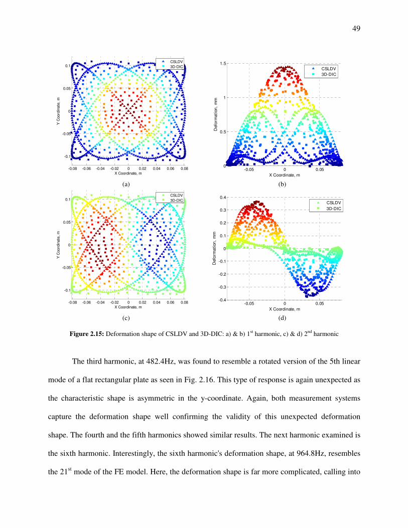
49

-0.08 -0.06 -0.04 -0.02 0 0.02 0.04 0.06 0.08

-0.1

-0.05

0

0.05

0.1

X Coordinate, m

Y C

oord

inate

, m

CSLDV

3D-DIC

(a)

-0.05 0 0.050

0.5

1

1.5

X Coordinate, m

Defo

rma

tion

, m

m

CSLDV

3D-DIC

(b)

-0.08 -0.06 -0.04 -0.02 0 0.02 0.04 0.06 0.08

-0.1

-0.05

0

0.05

0.1

X Coordinate, m

Y C

oord

inate

, m

CSLDV

3D-DIC

(c)

-0.05 0 0.05-0.4

-0.3

-0.2

-0.1

0

0.1

0.2

0.3

0.4

X Coordinate, m

Defo

rma

tion

, m

m

CSLDV

3D-DIC

(d)

Figure 2.15: Deformation shape of CSLDV and 3D-DIC: a) & b) 1st harmonic, c) & d) 2

nd harmonic

The third harmonic, at 482.4Hz, was found to resemble a rotated version of the 5th linear

mode of a flat rectangular plate as seen in Fig. 2.16. This type of response is again unexpected as

the characteristic shape is asymmetric in the y-coordinate. Again, both measurement systems

capture the deformation shape well confirming the validity of this unexpected deformation

shape. The fourth and the fifth harmonics showed similar results. The next harmonic examined is

the sixth harmonic. Interestingly, the sixth harmonic's deformation shape, at 964.8Hz, resembles

the 21st mode of the FE model. Here, the deformation shape is far more complicated, calling into

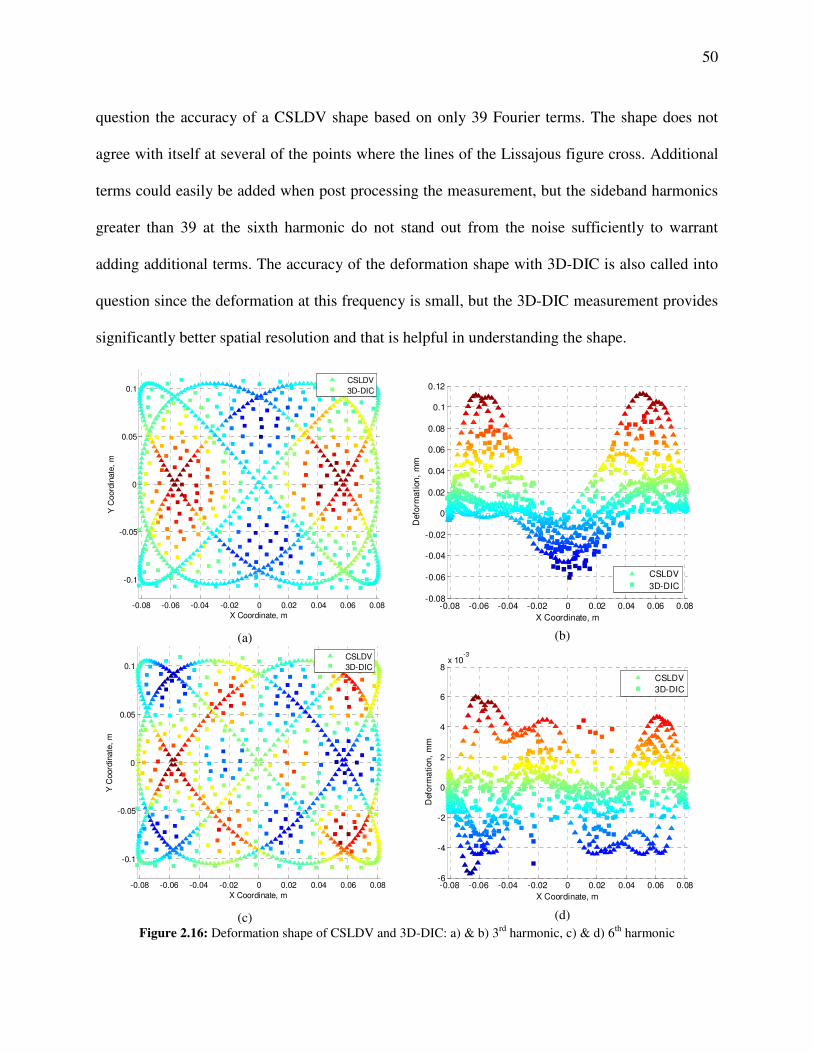
50

question the accuracy of a CSLDV shape based on only 39 Fourier terms. The shape does not

agree with itself at several of the points where the lines of the Lissajous figure cross. Additional

terms could easily be added when post processing the measurement, but the sideband harmonics

greater than 39 at the sixth harmonic do not stand out from the noise sufficiently to warrant

adding additional terms. The accuracy of the deformation shape with 3D-DIC is also called into

question since the deformation at this frequency is small, but the 3D-DIC measurement provides

significantly better spatial resolution and that is helpful in understanding the shape.

-0.08 -0.06 -0.04 -0.02 0 0.02 0.04 0.06 0.08

-0.1

-0.05

0

0.05

0.1

X Coordinate, m

Y C

oord

inate

, m

CSLDV

3D-DIC

(a)

-0.08 -0.06 -0.04 -0.02 0 0.02 0.04 0.06 0.08-0.08

-0.06

-0.04

-0.02

0

0.02

0.04

0.06

0.08

0.1

0.12

X Coordinate, m

Defo

rma

tion

, m

m

CSLDV

3D-DIC

(b)

-0.08 -0.06 -0.04 -0.02 0 0.02 0.04 0.06 0.08

-0.1

-0.05

0

0.05

0.1

X Coordinate, m

Y C

oord

inate

, m

CSLDV

3D-DIC

(c)

-0.08 -0.06 -0.04 -0.02 0 0.02 0.04 0.06 0.08-6

-4

-2

0

2

4

6

8x 10

-3

X Coordinate, m

Defo

rma

tion,

mm

CSLDV

3D-DIC

(d)

Figure 2.16: Deformation shape of CSLDV and 3D-DIC: a) & b) 3rd

harmonic, c) & d) 6th

harmonic

51

2.7 Summary

The mode shapes and natural frequencies of a clamped-clamped flat steel beam and a

fully clamped rectangular aluminum plate were identified using CSLDV and high speed 3D-

DIC. CSLDV was able to measure 1708 points across the surface of the beam and 10240 points

across the surface of the plate. However, the information in the measurement is not governed by

the number of points used to define the shape but by the number of Fourier coefficients that can

be identified to describe the time-varying shape. In fact, decreasing the sample rate, and hence

the number of sampled points, has sometimes been found to increase the resolution of the

measurement [72]. The number of harmonics is especially important when a more complex 2-D

measurement grid is used. Hence, the main disadvantage of CSLDV is that the harmonics

describing the shapes are measured rather than the shapes at individual points, and so there may

be uncertainty as to whether a feature in the measured deformation is really meaningful.

On the other hand, CSLDV offers a few benefits over high-speed 3D-DIC: CSLDV can

measure at large stand off distances, maintains accuracy over larger test specimens, and current

LDVs clearly have much higher measurement resolution than DIC, down to tens of nano-meter/s

velocities or pico-meter displacements. Some of that resolution can be lost to speckle noise when

scanning the laser, and this was observed in the measurement of higher modes for the plate in

this study, but even then CSLDV was shown to be more accurate than DIC when capturing the

small amplitude linear vibration of the beam and plate. For the (small-amplitude) higher

harmonics of the nonlinear response the results were mixed; while CSLDV did have a lower

noise floor the number of harmonics required to describe the motion increased significantly and

in some cases accurate shapes still could not be measured. Finally, one should note that the

52

quality of the CSLDV measurement depends on the type of laser, the surface quality, scanning

frequency and other parameters so while we expect these trends to hold, the relative performance

may be different for other structures.

High speed 3D-DIC was computed with 82 points for the beam and 300 points for the

plate; however, a denser measurement grid could have been obtained if needed since the images

were stored and post processed to obtain displacements. For the given field of view and

geometry, 2500 points can be computed in a 2D grid across the surface of the beam and the

measurement resolution is independent of measurement duration or excitation type. (In CSLDV,

the spatial information is captured in empty regions between the excitation frequencies lines in

the spectrum, and hence one must consider the input type, scan frequency, speckle noise, and the

properties of the system to successfully capture measurements.)

The spatial resolution of the acquired mode shape measured with high speed 3D-DIC is

dependent on the stand off distance and the camera resolution; therefore, if more accurate

measurements are needed, the camera setup needs to be moved closer to the test specimen, or a

higher resolution camera is needed. Additionally, since high frequencies correspond to smaller

displacements, high-speed 3D-DIC loses ability to measure mode shapes at higher frequencies.

One benefit high-speed 3D-DIC has over CSLDV is the ability to provide a 2D grid of

measurement points equally spaced across the specimen surface. CSLDV provided

measurements over a less optimal grid of points. Furthermore, 3D-DIC measures the three

dimensional deformations providing near full-field measurements in all deformation axes.

Indeed, with 3D-DIC one can capture the in-plane motions of the surface even more accurately

than the out-of-plane motions, whereas CSLDV can only capture the motion along the axis of the

53

incident laser beam. While the in-plane motions were still too small for 3D-DIC to resolve for

the flat structures investigated here, this feature could prove valuable for curved structures.

Both techniques can provide dense measurements along surfaces, as long as each

technique can "see" the surface. To provide accurate measurements, both techniques require

surface preparation, unless the material used for the test piece fulfills specific requirements (e.g.

a random pattern for 3D-DIC and a sufficiently reflective pattern for CSLDV). For DIC, this

surface preparation is especially important when response levels are small, or in a structure's

linear range. For CSLDV, surface preparation becomes more important when the vibration

amplitude becomes small relative to speckle noise, and also as the laser standoff distance (or

field of view) increases.

Finally, this study has illustrated that when full-field velocities or displacements are

measured (i.e. as opposed to the usual case where the motion is only captured at a few points),

inconsistencies in the dynamic behavior of the structure under test can be identified and provide

insight to modeling and predicting dynamic behavior. Here, the CSLDV and DIC shapes

revealed asymmetry in the 2nd and 3rd bending mode shapes of the beam and a skew in mode 1

of the bending mode shape of the plate, which was probably due to (un-modeled) asymmetry in

the boundary conditions or initial geometry of the plate since it is thin. If a traditional test were

performed with only a few measurement points, one would not be likely to detect this, nor would

they have sufficient information to update the model to account for it.

54

3 Experimental Identification of Nonlinear Normal Modes

This chapter was taken from a draft of a journal paper that will soon be submitted, and

as a result the first few paragraphs repeat some of the theory that was reviewed in the

introduction.

3.1 Introduction

Over the past several decades a suite of testing and modeling techniques has been

developed to quantify the dynamic motion of a structure using modal properties (eg. resonant

frequencies, mode shapes, and damping ratios) [5, 73, 74]. The measured or calculated modal

properties are typically used to quantify the inertial (mass), elastic (stiffness), and dissipation

(damping) characteristics of a structure. Modal properties provide the benefit of describing

global dynamics of a structure with a small number of physical degrees of freedom (DOF) due to

several attributes inherent to their determination (eg. orthogonality, invariance, and

superposition). Linear Normal Modes (LNMs) are built on the assumption of linear force-

displacement relationships. The classical, undamped LNMs that are our focus here are a special

case of Complex Modes, and are only valid when the structure exhibits proportional damping or

when any coupling of the classical modes due to damping is negligible [75, 76]. The derivation

and further description of LNMs can be found in many engineering dynamics or vibrations

textbooks [76-79]. When a structure exhibits the nonlinear force-displacement relationships that

are typical under large amplitude loading conditions, the concepts behind LNMs break down,

the LNMs (e.g. those that could be defined for small deformations about some reference state)

become coupled and the resonance frequency shows a strong dependence on amplitude.

Therefore, testing and analysis techniques created around a structure's LNMs cannot be directly

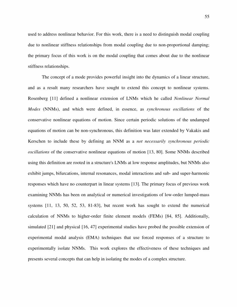
55

used to address nonlinear behavior. For this work, there is a need to distinguish modal coupling

due to nonlinear stiffness relationships from modal coupling due to non-proportional damping;

the primary focus of this work is on the modal coupling that comes about due to the nonlinear

stiffness relationships.

The concept of a mode provides powerful insight into the dynamics of a linear structure,

and as a result many researchers have sought to extend this concept to nonlinear systems.

Rosenberg [11] defined a nonlinear extension of LNMs which he called Nonlinear Normal

Modes (NNMs), and which were defined, in essence, as synchronous oscillations of the

conservative nonlinear equations of motion. Since certain periodic solutions of the undamped

equations of motion can be non-synchronous, this definition was later extended by Vakakis and

Kerschen to include these by defining an NNM as a not necessarily synchronous periodic

oscillations of the conservative nonlinear equations of motion [13, 80]. Some NNMs described

using this definition are rooted in a structure's LNMs at low response amplitudes, but NNMs also

exhibit jumps, bifurcations, internal resonances, modal interactions and sub- and super-harmonic

responses which have no counterpart in linear systems [13]. The primary focus of previous work

examining NNMs has been on analytical or numerical investigations of low-order lumped-mass

systems [11, 13, 50, 52, 53, 81-83], but recent work has sought to extend the numerical

calculation of NNMs to higher-order finite element models (FEMs) [84, 85]. Additionally,

simulated [21] and physical [16, 47] experimental studies have probed the possible extension of

experimental modal analysis (EMA) techniques that use forced responses of a structure to

experimentally isolate NNMs. This work explores the effectiveness of these techniques and

presents several concepts that can help in isolating the modes of a complex structure.

56

In EMA, the idea of identifying nonlinearity in the measurement of a structural response

is well understood since most techniques break down in the presence of nonlinear behavior [46].

EMA methodologies have therefore been developed to average out observed nonlinearities,

avoid nonlinear behavior, or to fit a linear model that approximates the nonlinear behavior of the

structure at a specific response amplitude. It must be noted that as experimental technologies

have improved accuracy, a much higher incidence of nonlinearity has been observed than in

previous years bringing the shortcomings of these linear EMA methodologies to light more

frequently [86]. EMA methodologies can be broadly split into two areas classified by the number

of LNMs measured during a test. Phase Resonance Methods (PRMs) excite one LNM at a time

by tuning the input force so that the measured response is the LNM of interest. Phase Separation

Methods (PSMs) excite multiple LNMs at a time with broadband excitation so that the LNMs

can be isolated from the measured response by using modal parameter estimation techniques.

There are certainly other classifications of modal analysis techniques that can provide a more

complete description of the concepts of EMA, but this classification is adequate for the

discussion that follows.

The most popular and easily implemented methods available today for EMA are PSMs,

where several or all LNMs of interest are excited simultaneously with the use of broadband

random, transient, or swept/stepped sine forcing. The modes of vibration are then isolated in

these measurements through the use of modal parameter estimation techniques. A good

reference for this type of testing and analysis can be found in [5, 73]. In the presence of

nonlinearity, PSMs break down in the parameter estimation step since the response no longer has

the mathematical form expected for a linear system. The extension of the parameter

identification step in PSMs to nonlinear regimes has seen much attention [18, 46]. This is by no

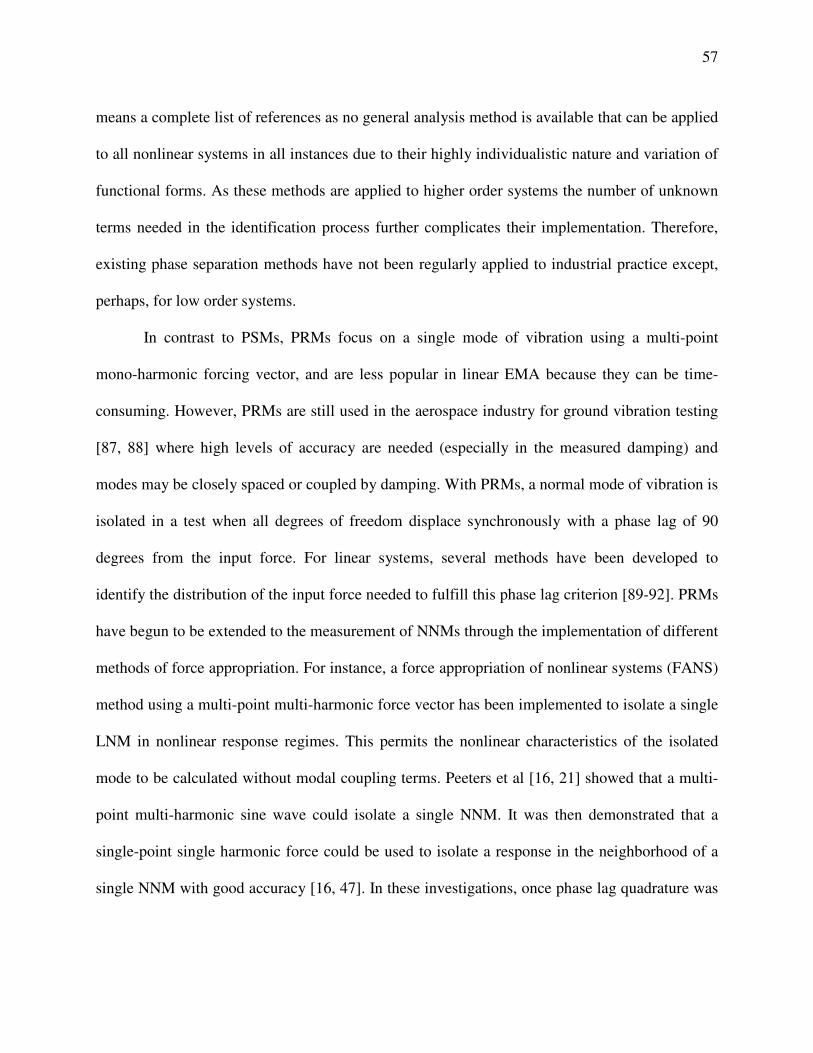
57

means a complete list of references as no general analysis method is available that can be applied

to all nonlinear systems in all instances due to their highly individualistic nature and variation of

functional forms. As these methods are applied to higher order systems the number of unknown

terms needed in the identification process further complicates their implementation. Therefore,

existing phase separation methods have not been regularly applied to industrial practice except,

perhaps, for low order systems.

In contrast to PSMs, PRMs focus on a single mode of vibration using a multi-point

mono-harmonic forcing vector, and are less popular in linear EMA because they can be time-

consuming. However, PRMs are still used in the aerospace industry for ground vibration testing

[87, 88] where high levels of accuracy are needed (especially in the measured damping) and

modes may be closely spaced or coupled by damping. With PRMs, a normal mode of vibration is

isolated in a test when all degrees of freedom displace synchronously with a phase lag of 90

degrees from the input force. For linear systems, several methods have been developed to

identify the distribution of the input force needed to fulfill this phase lag criterion [89-92]. PRMs

have begun to be extended to the measurement of NNMs through the implementation of different

methods of force appropriation. For instance, a force appropriation of nonlinear systems (FANS)

method using a multi-point multi-harmonic force vector has been implemented to isolate a single

LNM in nonlinear response regimes. This permits the nonlinear characteristics of the isolated

mode to be calculated without modal coupling terms. Peeters et al [16, 21] showed that a multi-

point multi-harmonic sine wave could isolate a single NNM. It was then demonstrated that a

single-point single harmonic force could be used to isolate a response in the neighborhood of a

single NNM with good accuracy [16, 47]. In these investigations, once phase lag quadrature was

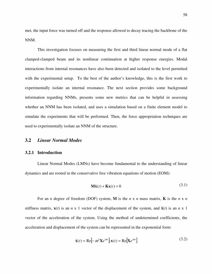
58

met, the input force was turned off and the response allowed to decay tracing the backbone of the

NNM.

This investigation focuses on measuring the first and third linear normal mode of a flat

clamped-clamped beam and its nonlinear continuation at higher response energies. Modal

interactions from internal resonances have also been detected and isolated to the level permitted

with the experimental setup. To the best of the author’s knowledge, this is the first work to

experimentally isolate an internal resonance. The next section provides some background

information regarding NNMs, presents some new metrics that can be helpful in assessing

whether an NNM has been isolated, and uses a simulation based on a finite element model to

simulate the experiments that will be performed. Then, the force appropriation techniques are

used to experimentally isolate an NNM of the structure.

3.2 Linear Normal Modes

3.2.1 Introduction

Linear Normal Modes (LMNs) have become fundamental to the understanding of linear

dynamics and are rooted in the conservative free vibration equations of motion (EOM):

0)()( =+ tt KxxM && (3.1)

For an n degree of freedom (DOF) system, M is the n x n mass matrix, K is the n x n

stiffness matrix, x(t) is an n x 1 vector of the displacement of the system, and ẍ(t) is an n x 1

vector of the acceleration of the system. Using the method of undetermined coefficients, the

acceleration and displacement of the system can be represented in the exponential form:

[ ] [ ]titi etet ωωω XxXx Re)(;Re)( 2 =−=&& (3.2)

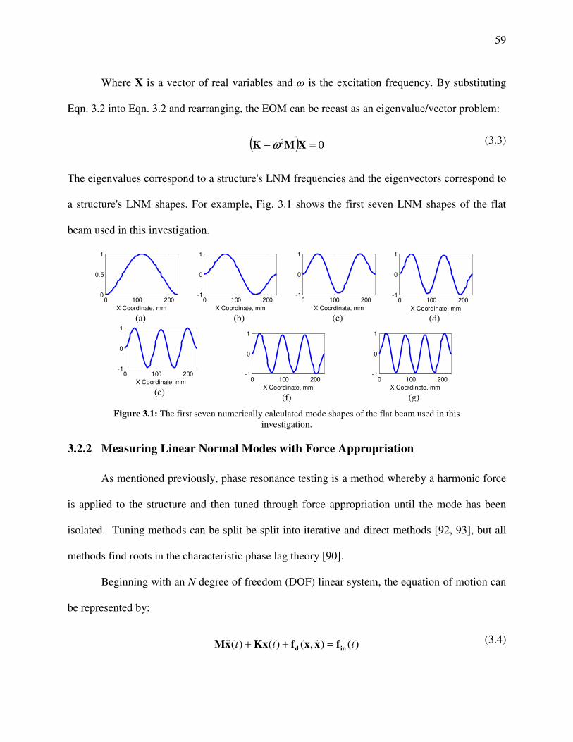
59

Where X is a vector of real variables and ω is the excitation frequency. By substituting

Eqn. 3.2 into Eqn. 3.2 and rearranging, the EOM can be recast as an eigenvalue/vector problem:

( ) 02 =− XMK ω (3.3)

The eigenvalues correspond to a structure's LNM frequencies and the eigenvectors correspond to

a structure's LNM shapes. For example, Fig. 3.1 shows the first seven LNM shapes of the flat

beam used in this investigation.

0 100 2000

0.5

1

X Coordinate, mm (a)

0 100 200-1

0

1

X Coordinate, mm (b)

0 100 200-1

0

1

X Coordinate, mm (c)

0 100 200-1

0

1

X Coordinate, mm

(d)

0 100 200-1

0

1

X Coordinate, mm (e)

0 100 200-1

0

1

X Coordinate, mm (f)

0 100 200-1

0

1

X Coordinate, mm (g)

Figure 3.1: The first seven numerically calculated mode shapes of the flat beam used in this

investigation.

3.2.2 Measuring Linear Normal Modes with Force Appropriation

As mentioned previously, phase resonance testing is a method whereby a harmonic force

is applied to the structure and then tuned through force appropriation until the mode has been

isolated. Tuning methods can be split be split into iterative and direct methods [92, 93], but all

methods find roots in the characteristic phase lag theory [90].

Beginning with an N degree of freedom (DOF) linear system, the equation of motion can

be represented by:

)(),()()( ttt ind fxxfKxxM =++ &&& (3.4)

60

Where M is the mass matrix, K is the stiffness matrix, fd is the vector of damping forces

that depend on the response of the structure, fin(t) is the input force vector and ẍ(t), ẋ(t), and x(t)

describe the structure's response. Using the method of undetermined coefficients, the structural

response to a harmonic excitation is also assumed to be harmonic. Therefore, it can be assumed

that the response and input force shown in Eqn. 3.4, take the forms:

( )[ ] ( )[ ] ( )[ ]tititi etetet ωθωθωω inin FfXxXx Re)(;Re)(;Re)( 2 ==−= −−&&

(3.5)

Where X and Fin and are vectors of real force and response amplitudes, respectively,

variables, ω is the excitation frequency, and θ is the phase lag of the response to the force (all

response coordinates also have the same phase lag). There are several forms fd can take

depending on the dissipation characteristics expected in the structure investigated (e.g. a beam

[94]). Two common forms of damping are viscous and structural, which have the following

form:

( ) ( )[ ]θωθωω −− += titieiei DXCXfd Re

(3.6)

Where iωC is related to viscous damping and iD is related to structural damping, and

both are 90 degrees out of phase from the response do the i term in each expression. As a results,

both are proportional to a structure's velocity. If only one type of damping is assumed, C or D

could be set to zero and the general form of damping, fd, would only contain the remaining

damping characteristics. Using the definitions established in Eqns. 3.5 and 3.6, Eqn. 3.4 can be

separated into imaginary and real parts with the phase in the complex exponential separated into

sine and cosine terms.

( )[ ] 0cossin2 =−− XFMK d θθω (3.7)

61

( )[ ] ind FXFMK =+− θθω sincos2 (3.8)

As discussed by de Veubeke [90], when the response has a delay of 90 degrees with the

input force vector, Eqn. 3.7 only contains the relationship between the stiffness and mass of the

structure and Eqn. 3.8 only contains the effect from damping, which is balanced by the input

force vector. For this phase criterion, the excitation frequency is at the undamped natural

frequency of the structure, ω = ωn, and the mono-phased response displacement, x, is the Normal

Mode shape.

Before proceeding to discuss nonlinear systems, it is beneficial to examine force that

must be applied to isolate a linear mode using the energy balancing technique [95-97]. If the

system is oscillating on a LNM, the power dissipated at any instant is:

)()( T

ttdiss xCxP &&= (3.9)

and the total energy dissipated for one period of response is:

∫∫ ==

TT

disscycdiss dtttdtE0

T

0

/ )()( xCxP &&

(3.10)

For an input forcing function fin(t), the energy the external force inputs into the system is:

∫=

T

cycin dtttE0

T

/ )()( infx&

(3.11)

At resonance the energy dissipated by the damping forces must equal the total energy

input to the system over the period T:

cycincycdiss EE // = (3.12)

62

For a structure with well separated modes, a single-point mono-harmonic force is all that

is needed to isolate a LNM. Note that such a force is not necessarily a good approximation to the

dissipative forces in the structure, but this works because the total energy input per cycle matches

the energy dissipated and the energy absorbed by modes other than the mode of interest ends up

being very small. In this context, when a single-point, mono-harmonic force is applied at a

location n on the structure, with amplitude A, the energy balance criterion in the equation above

becomes:

∫∫ =

T

ti

n

T

dtetAdttt0

T

0

T )()()( ωxxCx &&&

(3.13)

This energy balancing criterion provides a direct link from the computed LNMs to the

resonant response of the damped forced system [97]. In an experiment, the tuning of an input

force vector to fully appropriate a normal mode, or cancel damping in the structure, is not easily

accomplished due to the difficulty in correctly modeling the damping and restrictions based on

the experimental setup. An in situ "hard tuning" of the mode is sometimes needed to bring the

isolated mode to some specified level of accuracy increasing the required test time to fully

appropriate a mode. An overview and comparison of various force appropriation methods can be

found in [92].

3.3 Nonlinear Normal Modes

3.3.1 Introduction

Similar to the LNMs previously introduced, the NNM definition used in this work is

rooted in the conservative nonlinear free vibration EOM:

63

0),,:,()()( =++ xxxxxfKxxM nltt&& (3.14)

In addition to the terms in Eqn. 3.1, fnl is the nonlinear restoring force which is purely a

function of displacement (e.g. including only stiffness terms). The nonlinear restoring force can

be represented by many functional forms depending on the type of nonlinearity expected (e.g.

polynomial stiffness and damping, clearances, impacts, friction, and saturation effects). For the

pure geometric nonlinearity expected in the beam investigated here, a polynomial function can

be used to describe the nonlinear stiffness. For example, a second order polynomial corresponds

to a spring softening effect or decrease in the fundamental frequency of vibration for increasing

energy levels, and a third order polynomial corresponds to a spring hardening effect or an

increase in fundamental frequency. The clamped-clamped flat beam examined in this work

exhibits a nonlinear restoring force that could contain both cubic and quadratic terms as

expressed in Eqn. 3.15, both of which come about due to coupling between bending and axial

stretching. The EOM becomes more complicated as additional DOF are included, since the

polynomials need to include cross terms between all pairs of DOF (e.g. b12x1x2, see [71, 98] for a

more thorough treatment).

),,(),(),,:,( xxxxx baxxxxxfnl += (3.15)

3.3.2 Numerical Example of NNM

Prior to testing, a finite element model (FEM) was created for the flat clamped-clamped

beam studied here and in [52]. Several methods have been developed to calculate the NNMs [53,

82] of a finite element models such as this; the numerical results presented here are calculated

using the applied modal force numerical continuation technique [52].

64

For convenience, 'families' of NNMs can be presented in frequency-energy plots (FEPs)

based on the fundamental frequency of the response and total energy conserved over a period of

the response. Three distinct 'families' of NNMs of the flat beam will be discussed in this chapter.

The first 'family' corresponds to the nonlinear continuation of LNM-1, or the backbone of NNM-

1 and is shown in Fig. 3.2a in blue. The second 'family' corresponds to a 5:1 harmonic coupling

between LNM-1 and LNM3, or an internally resonant NNM-1-3 and is shown in Fig. 3.2a in red.

As seen in the FEP presented in Fig. 3.2a, the flat beam exhibits a spring hardening nonlinearity,

or an increase in the fundamental frequency of vibration with increased input energy as discussed

in [71, 99]. This figure captures a 36% change in the fundamental frequency of vibration in

NNM-1, shown in blue, and this large change is observed for relatively small response energies.

For reference, a demarcation is added to these plots showing where the maximum displacement

amplitude of the beam would be equal to one thickness (e.g. 0.76mm).

Throughout the blue curve (Fig. 3.2b), the LNM-1 dominates the response of the flat

beam, although a small broadening of the deformation shape is observed at higher energies due

to axial stretching of the beam. Along the red curve (Fig. 3.2b), the deformation shape seems to

contain a contribution from LNM-3 at higher energies due to the coupling between NNM-1 and

NNM-3. This can be verified through the examination of the deformation of the beam throughout

a quarter period of the response (Figs. 3.2c-e) and of the Fourier coefficients of the response

(Figs. 3.2f-h). As seen in Figs. 3.2c and 3.2e, which corresponds to Points 1 and 3 marked on the

FEP, the LNM-1 dominates the deformation shape and there are minimal contributions from

higher harmonics as Figs. 3.2f and 3.2g. The FFT and deformation at Point 2 on the IR branch of

NNM-1 are shown in Figs. 3.2d and 3.2g. As the fifth harmonic begins to increase at larger

amplitude responses further up the IR branch of NNM-1, the deformation begins to resemble a

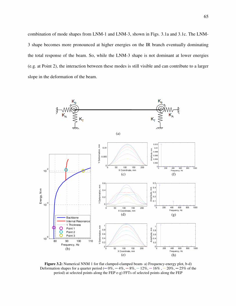
65

combination of mode shapes from LNM-1 and LNM-3, shown in Figs. 3.1a and 3.1c. The LNM-

3 shape becomes more pronounced at higher energies on the IR branch eventually dominating

the total response of the beam. So, while the LNM-3 shape is not dominant at lower energies

(e.g. at Point 2), the interaction between these modes is still visible and can contribute to a larger

slope in the deformation of the beam.

(a)

0 50 100 150 2000

0.005

0.01

X Coordinate, mm

Y D

efo

rmation,

mm

(c)

0 200 400 600 800 10000

0.002

0.004

0.006

0.008

0.01

0.012

Frequency, Hz

Am

plitu

de

, m

m

(f)

0 50 100 150 200

0

0.2

0.4

0.6

X Coordinate, mm

Y D

efo

rmati

on,

mm

(d)

0 200 400 600 800 10000

0.1

0.2

0.3

0.4

0.5

Frequency, Hz

Am

pli

tud

e,

mm

(g)

10-6

10-4

10-2

80 90 100 110

Frequency, Hz

Ene

rgy,

N-m

Backbone

Internal Resonance

1 Thickness

Point 1

Point 2

Point 3

(b)

0 50 100 150 2000

0.2

0.4

0.6

0.8

1

X Coordinate, mm

Y D

efo

rmati

on,

mm

(e)

0 200 400 600 800 10000

0.2

0.4

0.6

0.8

1

Frequency, Hz

Am

pli

tud

e,

mm

(h)

Figure 3.2: Numerical NNM 1 for flat clamped-clamped beam- a) Frequency-energy plot, b-d)

Deformation shapes for a quarter period (─ 0%, ─ 4%, ─ 8%, ─ 12%, ─ 16% , ─ 20%, ─ 25% of the

period) at selected points along the FEP e-g) FFTs of selected points along the FEP

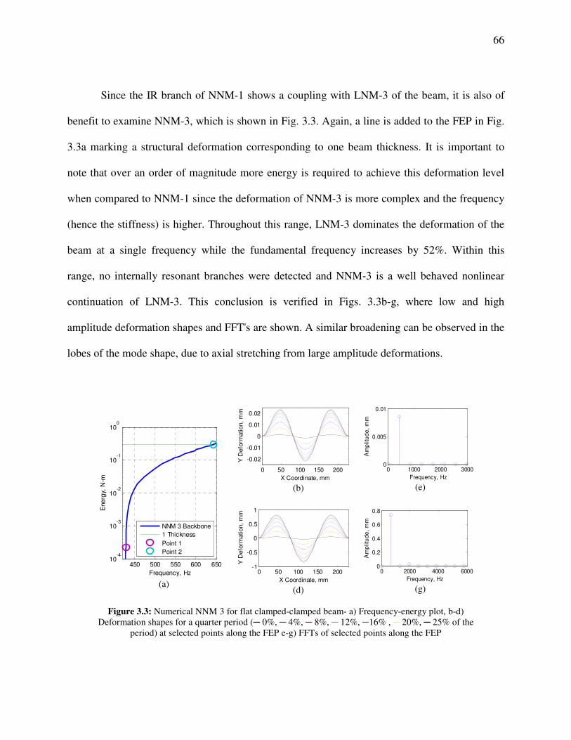
66

Since the IR branch of NNM-1 shows a coupling with LNM-3 of the beam, it is also of

benefit to examine NNM-3, which is shown in Fig. 3.3. Again, a line is added to the FEP in Fig.

3.3a marking a structural deformation corresponding to one beam thickness. It is important to

note that over an order of magnitude more energy is required to achieve this deformation level

when compared to NNM-1 since the deformation of NNM-3 is more complex and the frequency

(hence the stiffness) is higher. Throughout this range, LNM-3 dominates the deformation of the

beam at a single frequency while the fundamental frequency increases by 52%. Within this

range, no internally resonant branches were detected and NNM-3 is a well behaved nonlinear

continuation of LNM-3. This conclusion is verified in Figs. 3.3b-g, where low and high

amplitude deformation shapes and FFT's are shown. A similar broadening can be observed in the

lobes of the mode shape, due to axial stretching from large amplitude deformations.

0 50 100 150 200

-0.02

-0.01

0

0.01

0.02

X Coordinate, mm

Y D

efo

rmatio

n,

mm

(b)

0 1000 2000 30000

0.005

0.01

Frequency, Hz

Am

plitu

de

, m

m

(e)

450 500 550 600 65010

-4

10-3

10-2

10-1

100

Ene

rgy,

N-m

Frequency, Hz

NNM 3 Backbone

1 Thickness

Point 1

Point 2

(a)

0 50 100 150 200-1

-0.5

0

0.5

1

X Coordinate, mm

Y D

efo

rmatio

n,

mm

(d)

0 2000 4000 60000

0.2

0.4

0.6

0.8

Frequency, Hz

Am

plitu

de

, m

m

(g)

Figure 3.3: Numerical NNM 3 for flat clamped-clamped beam- a) Frequency-energy plot, b-d)

Deformation shapes for a quarter period (─ 0%, ─ 4%, ─ 8%, ─ 12%, ─16% , ─ 20%, ─ 25% of the

period) at selected points along the FEP e-g) FFTs of selected points along the FEP

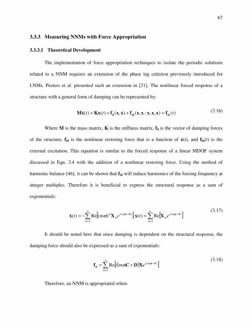
67

3.3.3 Measuring NNMs with Force Appropriation

3.3.3.1 Theoretical Development

The implementation of force appropriation techniques to isolate the periodic solutions

related to a NNM requires an extension of the phase lag criterion previously introduced for

LNMs. Peeters et al. presented such an extension in [21]. The nonlinear forced response of a

structure with a general form of damping can be represented by:

)(),,:,(),()()( ttt innld fxxxxxfxxfKxxM =+++ &&& (3.16)

Where M is the mass matrix, K is the stiffness matrix, fd is the vector of damping forces

of the structure, fnl is the nonlinear restoring force that is a function of x(t), and fin(t) is the

external excitation. This equation is similar to the forced response of a linear MDOF system

discussed in Eqn. 3.4 with the addition of a nonlinear restoring force. Using the method of

harmonic balance [46], it can be shown that fnl will induce harmonics of the forcing frequency at

integer multiples. Therefore it is beneficial to express the structural response as a sum of

exponentials:

[ ] [ ]∑∑

∞

=

−∞

=

− =−=1

)(

1

)(2 Re)(;)(Re)(m

tmi

m

m

tmi

m etemtθωθωω XxXx&&

(3.17)

It should be noted here that since damping is dependent on the structural response, the

damping force should also be expressed as a sum of exponentials:

( )[ ]∑

∞

=

−+=1

)(Rem

tmiemi

θωω XDCfd

(3.18)

Therefore, an NNM is appropriated when:

68

)(),( tind fxxf =& (3.19)

Simply stated, the response of a structure is on the NNM when the forcing function

exactly cancels the damping forces in the structure for all harmonics. In practice one cannot

apply a force that exactly cancels damping, so one wishes to apply a force that approximately

isolates an NNM and this can be computed using the energy balancing techniques [96, 97] that

was previously discussed. Returning to Eqn. (3.11), the mono-harmonic input force, fin(t), can be

expanded to a multi-harmonic force

( )1

sin( )

0

N

k

kj

A k t j nt

j n

ω=

=

= ≠

∑inf (3.20)

where n is the point at which the force is applied and ()j denotes the jth element of the vector.

Because the sine function are orthogonal over the fundamental period, T, when this is

inserted into the expression for Ein/cyc , one obtains a sum of terms that give the contribution of

each harmonic to Ein/cyc. Substituting this back into Eqn. (3.13) yields:

∑ ∫∫=

=N

k

T

tik

nk

T

dtetAdttt1 0

*

0

* )()()( ωxxCx &&&

(3.21)

In summary, given the known NNM motion, ẋ(t), and damping matrix, C, the multi-point

damping force, Cẋ, can be computed. From this, coefficients, Ak, of a multi-harmonic, single-

point force can be determined that would input the same energy per cycle when the structure

oscillates in the NNM of interest. This method was used numerically to determine the forced

responses needed to isolate a NNM in simulation. In practice the NNM is not known a priori, so

we wish to tune the input until an NNM is isolated. We seek a strategy whereby successive

69

changes in the amplitude and fundamental frequency the input force can be made that isolates an

NNM of interest.

For either of the damping models previously described, the damping force lags the

displacement of the structure by 90 degrees, or it will be in phase with the structure's velocity.

Additionally, measuring the input force and response velocity can often both be measured at the

point at which the structure is excited. Returning to Eqn. 3.19, na NNM is appropriated when the

input force is equal to the damping forces in the structure, or when the measured input force is

exactly 180° out of phase with the measured velocity. It is important to note that although a

mathematical model of damping can be assumed, the scaling factor of the damping force is not

known a priori, so only the phase information can be used in situ. This force-velocity

relationship is easy to monitor in a test and guides the determination of the amplitude and

frequency distribution of the force as will be shown both the simulation and experimental results

that follow. In order to find a the evolution of an NNM along a branch, this appropriation process

can be repeated at subsequent frequency and amplitude levels until the branch of the desired

NNM is identified. Since each point along the NNM corresponds to a time invariant periodic

response of the structure, the measured time series can be decomposed using a discrete Fourier

transform (if the sample increment and period are carefully chosen, or using least squares to

solve for the Fourier coefficients, as was done here).

The proposed technique to determine the frequency and amplitude distribution of the

force vector strongly depends on the assumption that the dissipative forces are solely dependent

on the velocity of the structural response. Therefore it is important to verify the quality of the

appropriated response independent of the force applied to the system. For linear structures, the

appropriated response is checked using a modal indicator function [92, 100]:

70

{ } { }{ } { }ZZ

ZZT

TReRe

=∆

(3.22)

Where Z is the complex Fourier coefficient vector of the response. This indicator has

been generalized to NNMs, termed the NNM Appropriation Indicator (NNMAI) [16]:

{ } { }{ } { }

∑=

=∆HN

k k

T

k

k

T

k

H

NNMZZ

ZZ

N 1

ReRe1 (3.23)

Where NH is the number of harmonics included in the indicator. For a perfectly

appropriated mode ∆ will give a value of 1 for both indicators.

3.3.3.2 Numerical Example of Stepped Sine Measurement of NNM

This can be demonstrated numerically for the beam previously described by computing

the forced response as a NNMs is approached. A Modified Crisfield integration technique is used

to find the dynamic response of the beam subjected to a single point input at the center of the

beam. For this numerical demonstration, linear modal damping ratios were identified

experimentally and applied to the model to create a linear modal damping matrix; the damping is

assumed not to change throughout the test. By monitoring the input force and velocity at the

center of the beam, one can tell that a mode has been isolated when the area of the input force-

velocity goes to zero. This is shown near the three points identified on the numerical NNM as

they represent a linear case (Point 1), an internally resonant case (Point 2), and a strongly

nonlinear case (Point 3). The results for Point 1 can be seen in Fig. 3.4. In addition to the

force/velocity relationship in Fig. 3.4a, MIFs have been calculated for the fundamental frequency

of the input and response and are given in the figure's caption. The phases of each harmonic are

71

provided in Tab. 3.1 and will be discussed subsequently. Each line color corresponds to an

increase in input frequency until the MIF is close to 1, while the input force amplitude is held

constant. As seen in Fig. 3.4a and 3.4b, with the increase in frequency, the response amplitude

increases. Since Point 1 is the near linear case, the higher harmonic content is minimal and the

force/velocity relationship appears to be linear once the NNM is isolated. For comparison with

Fig. 3.4b, the deformation over a quarter of a cycle is shown in Fig. 3.4c and is dominated by the

LNM-1 shape.

-5 0 5

-2

-1

0

1

2

x 10-4

Velocity, mm/s

Forc

e,

N

(a)

0 200 400 6000

5

10

Frequency, Hz

mm

/s

0 200 400 6000

2

4x 10

-4

Frequency, Hz

N

(b)

0 50 100 150 2000

0.005

0.01

0.015

0.02

X Coordinate, mm

Y C

oord

inate

, m

m

(c)

Figure 3.4: Appropriated force for Point 1 on NNM-1. a) Input force versus response velocity and b)

Amplitude of force and velocity Fourier coefficients at steps along the forced response of the beam for

increasing MIF values (∆): ─ 0.7456, ─ 0.9034, ─ 0.9931, ─ 0.9999, c) Deformation shapes for a quarter

period (─ 0%, ─ 4%, ─ 8%, ─ 12%, ─16% , ─ 20%, ─ 25% of the period)

72

Continuing on to Point 2, which is the internal resonance, a strong coupling is observed

between LNM-1 and LNM-3 as previously discussed. The steady-state responses for a single-

input multi-harmonic forcing amplitude as the frequency is increased are shown in Fig. 3.5. A

nonlinear force/velocity relationship is observed in Fig. 3.5a, and once again the area enclosed

by the curve decreases as the response approaches the true NNM as evidenced by the MIFs that

are given in the figure's caption. The total deformation of the response, shown in Fig. 3.5c,

resembles the deformation shape shown in Fig. 3.2c.

-400 -200 0 200 400-0.01

-0.005

0

0.005

0.01

Velocity, mm/s

Forc

e, N

(a)

0 100 200 300 400 5000

100

200

300

Frequency, Hz

mm

/s

0 100 200 300 400 5000

0.005

0.01

Frequency, Hz

N

(b)

0 50 100 150 200-0.1

0

0.1

0.2

0.3

0.4

0.5

0.6

X Coordinate, mm

Y C

oord

inate

, m

m

(c)

Figure 3.5: Appropriated force for Point 2. a) Input force versus response velocity and b) Amplitude of

force and velocity Fourier coefficients at steps along the forced response of the beam at increasing MIF

values (∆): ─ 0.5153, ─ 0.7747, ─ 0.9933, c) Deformation shapes for a half of a period (─ 0%, ─ 4%, ─

7%, ─ 11%, ─14% , ─ 18%, ─ 25%) of the period

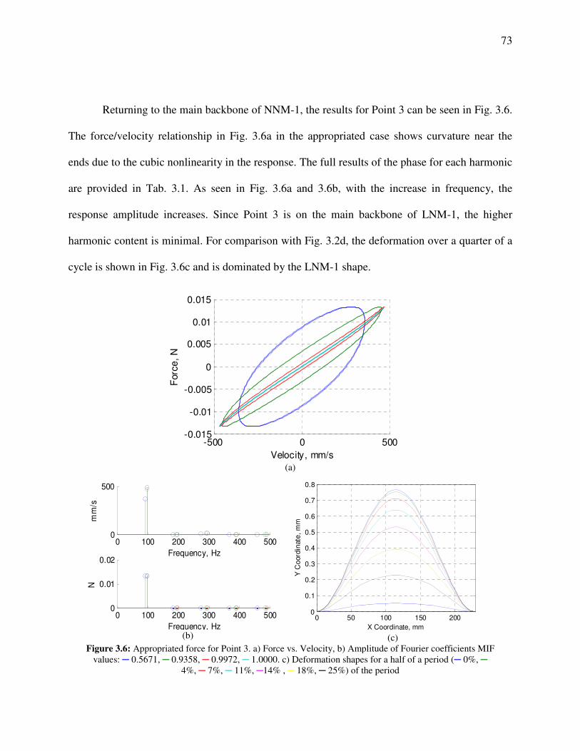
73

Returning to the main backbone of NNM-1, the results for Point 3 can be seen in Fig. 3.6.

The force/velocity relationship in Fig. 3.6a in the appropriated case shows curvature near the

ends due to the cubic nonlinearity in the response. The full results of the phase for each harmonic

are provided in Tab. 3.1. As seen in Fig. 3.6a and 3.6b, with the increase in frequency, the

response amplitude increases. Since Point 3 is on the main backbone of LNM-1, the higher

harmonic content is minimal. For comparison with Fig. 3.2d, the deformation over a quarter of a

cycle is shown in Fig. 3.6c and is dominated by the LNM-1 shape.

-500 0 500-0.015

-0.01

-0.005

0

0.005

0.01

0.015

Velocity, mm/s

Forc

e,

N

(a)

0 100 200 300 400 5000

500

Frequency, Hz

mm

/s

0 100 200 300 400 5000

0.01

0.02

Frequency, Hz

N

(b)

0 50 100 150 2000

0.1

0.2

0.3

0.4

0.5

0.6

0.7

0.8

X Coordinate, mm

Y C

oord

inate

, m

m

(c)

Figure 3.6: Appropriated force for Point 3. a) Force vs. Velocity, b) Amplitude of Fourier coefficients MIF

values: ─ 0.5671, ─ 0.9358, ─ 0.9972, ─ 1.0000. c) Deformation shapes for a half of a period (─ 0%, ─

4%, ─ 7%, ─ 11%, ─14% , ─ 18%, ─ 25%) of the period

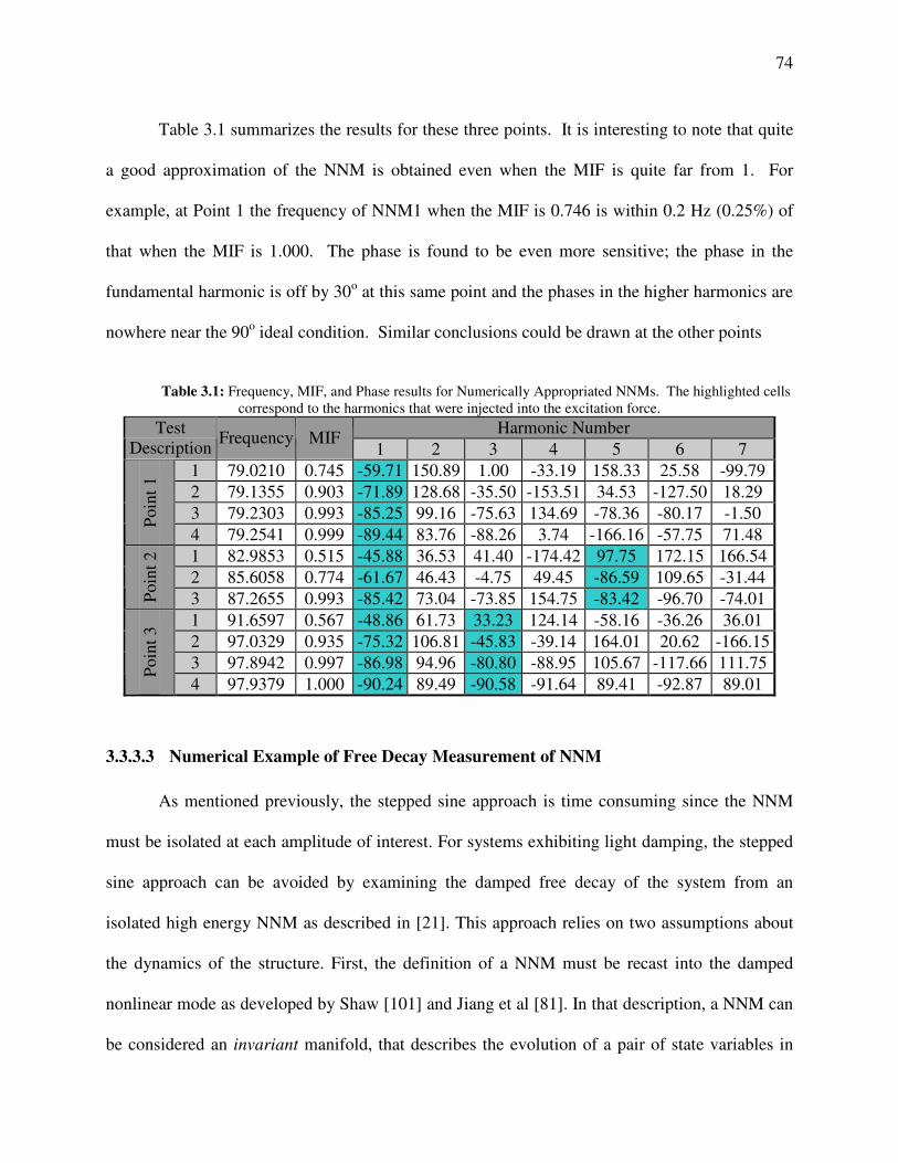
74

Table 3.1 summarizes the results for these three points. It is interesting to note that quite

a good approximation of the NNM is obtained even when the MIF is quite far from 1. For

example, at Point 1 the frequency of NNM1 when the MIF is 0.746 is within 0.2 Hz (0.25%) of

that when the MIF is 1.000. The phase is found to be even more sensitive; the phase in the

fundamental harmonic is off by 30o at this same point and the phases in the higher harmonics are

nowhere near the 90o ideal condition. Similar conclusions could be drawn at the other points

Table 3.1: Frequency, MIF, and Phase results for Numerically Appropriated NNMs. The highlighted cells

correspond to the harmonics that were injected into the excitation force.

Harmonic Number Test

Description Frequency MIF

1 2 3 4 5 6 7

1 79.0210 0.745 -59.71 150.89 1.00 -33.19 158.33 25.58 -99.79

2 79.1355 0.903 -71.89 128.68 -35.50 -153.51 34.53 -127.50 18.29

3 79.2303 0.993 -85.25 99.16 -75.63 134.69 -78.36 -80.17 -1.50

Po

int

1

4 79.2541 0.999 -89.44 83.76 -88.26 3.74 -166.16 -57.75 71.48

1 82.9853 0.515 -45.88 36.53 41.40 -174.42 97.75 172.15 166.54

2 85.6058 0.774 -61.67 46.43 -4.75 49.45 -86.59 109.65 -31.44

Po

int

2

3 87.2655 0.993 -85.42 73.04 -73.85 154.75 -83.42 -96.70 -74.01

1 91.6597 0.567 -48.86 61.73 33.23 124.14 -58.16 -36.26 36.01

2 97.0329 0.935 -75.32 106.81 -45.83 -39.14 164.01 20.62 -166.15

3 97.8942 0.997 -86.98 94.96 -80.80 -88.95 105.67 -117.66 111.75

Po

int

3

4 97.9379 1.000 -90.24 89.49 -90.58 -91.64 89.41 -92.87 89.01

3.3.3.3 Numerical Example of Free Decay Measurement of NNM

As mentioned previously, the stepped sine approach is time consuming since the NNM

must be isolated at each amplitude of interest. For systems exhibiting light damping, the stepped

sine approach can be avoided by examining the damped free decay of the system from an

isolated high energy NNM as described in [21]. This approach relies on two assumptions about

the dynamics of the structure. First, the definition of a NNM must be recast into the damped

nonlinear mode as developed by Shaw [101] and Jiang et al [81]. In that description, a NNM can

be considered an invariant manifold, that describes the evolution of a pair of state variables in

75

linear modal phase space. (Note that to describe interactions of modes one must retain a pari of

coordinates, (e.g. modal displacement and velocity), for each mode involved in the NNM

response yet that is not considered in any of the works on the resonant decay method of which

the authors are aware). Due to the invariance property of these manifolds, a motion that initiates

on the defined manifold will remain on the manifold for all time. Only under these conditions

can one be assured that the response will not depart from the manifold of interest as the energy

decays. Second, the undamped NNM must be viewed as an attractor of the damped free response

of the system, so that motions that initiate near the undamped NNM are drawn to it and decay

along the manifold. Third, the damping should be light so that the damped manifold is well

approximated by the undamped manifold. Under these conditions the free decay of a system

initiated on a NNM can be considered an approximation of the undamped NNM. Since the time

series measurements of the free decay are time variant, more complex signal processing

techniques such as the Wavelet Transform [102] and Hilbert Transform [103] are needed. A

recent interesting contribution to this type of analysis can be found here [19].

Returning to the simulation results for the fully appropriated responses at Point 2 and

Point 3, the force used to cancel damping within the system is turned off and the response is

calculated as the system decays. The Wavelet Transform and the Hilbert Transform can be used

to describe this decaying response. Using the building Wavelet toolbox in MATLAB®, a Morlet

wavelet is selected as the base family for the wavelet analysis. For the decay corresponding to

the Point 2 appropriated NNM, the time series and the wavelet transform are presented in Figs.

3.7a and 3.7b. The Wavelet Transform, shown in Fig. 3.7b, shows two dominant frequencies in

the response at 85.91Hz and 430Hz corresponding to a 5:1 harmonic interaction of the response,

although the response of the fundamental harmonic is an order of magnitude larger than the fifth

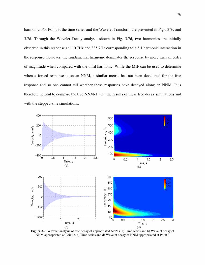
76

harmonic. For Point 3, the time series and the Wavelet Transform are presented in Figs. 3.7c and

3.7d. Through the Wavelet Decay analysis shown in Fig. 3.7d, two harmonics are initially

observed in this response at 110.7Hz and 335.7Hz corresponding to a 3:1 harmonic interaction in

the response; however, the fundamental harmonic dominates the response by more than an order

of magnitude when compared with the third harmonic. While the MIF can be used to determine

when a forced response is on an NNM, a similar metric has not been developed for the free

response and so one cannot tell whether these responses have decayed along an NNM. It is

therefore helpful to compare the true NNM-1 with the results of these free decay simulations and

with the stepped-sine simulations.

0 0.5 1 1.5 2 2.5-400

-200

0

200

400

Time, s

Velo

city,

mm

/s

(a)

(b)

0 1 2 3-1000

-500

0

500

1000

Time, s

Velo

city,

mm

/s

(c)

(d)

Figure 3.7: Wavelet analysis of free decay of appropriated NNMs. a) Time series and b) Wavelet decay of

NNM appropriated at Point 2. c) Time series and d) Wavelet decay of NNM appropriated at Point 3

77

3.3.3.4 Comparison of NNM Measurement Methods

Figure 3.8 compares the isolated NNM responses for the stepped-sine and free decay

experiments. The stepped-sine results were analyzed using Fourier series techniques and the

instantaneous amplitude and frequency of the decaying response was determined using the

Hilbert Transform. For the NNM-1 backbone, two decays were performed. Each decay was

initiated with the highest level of forcing amplitude, but at two different frequencies

corresponding to two different MIF values (1.000 and 0.5114) and therefore two levels of

accuracy in the appropriated forcing. The decay of the fully appropriated NNM-1 at Point 3 (MIF

= 1.000), is shown with a blue line and the decay of the partially appropriated response at Point 3

(MIF = 0.5114), is shown with the green line. Both decays overlay well showing the

effectiveness of the free decay in the isolation of NNM-1, even when the force does not perfectly

isolate the NNM. The blue and green circles show the starting points of each of these decays.

Two additional points were added, shown with cyan and magenta circles, corresponding to

NNMs that were isolated by iterating on the stepped sine input until a high MIF value was

obtained. This response appears to backbone of NNM-1 through the internal resonance branch

presented in Fig. 3.2. The third decay, shown in red, corresponds to the decay of the response off

of the IR branch of NNM-1. The starting point of this decay is shown as a red circle. It is

interesting to note that this decaying response does not solely decay on the internal resonance

branch (at 430Hz) before following the backbone of NNM-1, but instead follows a different path

with a dominant frequency closer to the NNM-1 backbone until settling onto LNM-1. This

illustrates a limitation to the free decay technique when the NNM exhibits strong modal coupling

as additional forcing is potentially need to follow the IR branch of NNM-1.

78

75 80 85 90 95 100 105 110 115

101

102

103

Frequency, Hz

Am

plitu

de

, m

m/s

Decay, MIF = 1.0000

Decay, MIF = 0.5114

Decay, MIF = 0.9933

Steady, MIF = 1.0000

Steady, MIF = 0.5114

Steady, MIF = 0.9933

Steady, MIF = 1.0000

Steady, MIF = 0.9999

Steady, MIF = 0.7456

Figure 3.8: Comparison of NNM measurement techniques.

3.4 Application to Clamped-Clamped Flat Beam with Geometric Nonlinearity

3.4.1 Flat Beam Description

The structure used for this investigation is a precision-machined feeler gauge made from

high-carbon, spring-steel in a clamped-clamped configuration previously studied in [67]. The

beam has a nominal effective length of 228mm, a width of 12mm, and a thickness of 0.76mm. It

is important to note that all presented dimensions are nominal and subject to variation from

clamping and stress variations from machining process to obtain the desired thickness. Prior to

clamping, the beam was prepared for three dimensional digital image correlation (3D-DIC) and

continuous-scan laser Doppler vibrometry (CSLDV) as discussed in [42] and shown in Fig. 3.9.

The clamping force was provided by four 6.35-28 UNF-2B bolts tightened to 9 N-m from left to

right. After clamping the beam to the fixture, a single-input single-output modal hammer test was

79

performed on the beam so linear natural frequencies and damping ratios could be identified as

well as a static 3D-DIC measurement so any initial geometry variations could be identified.

Additionally, operational modal analysis and CSLDV [63] were used to determine the mode

shapes of the beam. Results of the natural frequencies and damping ratios of the first ten modes

identified from the modal hammer test are shown in Tab. 3.2, and results of the first seven elastic

bending mode shapes are shown in Fig. 3.10. In Fig. 3.10, forward and backward sweeps of the

CSLDV setup were used independently to reconstruct the mode shapes, so deviations between

the two measurements give an indication of error in the measured shapes. For example, the lower

left lobe of the third mode shape shows a small difference between the forward and backward

sweep reconstructed shape indicating a deviation in the isolated mode. Since these errors are

relatively small, the two shapes are averaged, and the new averaged shape is used to decompose

the nonlinear CSLDV measurements as shown in the results section.

Figure 3.9: Beam Specimen

Table 3.2: Linear (low amplitude) natural frequencies of flat clamped-clamped beam

Mode

1

Mode

2

Mode

3

Mode

4

Mode

5

Mode

6

Mode

7

Mode

8

Mode

9

Mode

10

f, Hz 45.8 171.6 371.7 638.7 973.7 1376.5 1847.7 2387.2 2586.5 2994.7

ζ1 , % 0.38 0.12 0.09 0.08 0.08 0.07 0.06 0.06 0.04 0.06

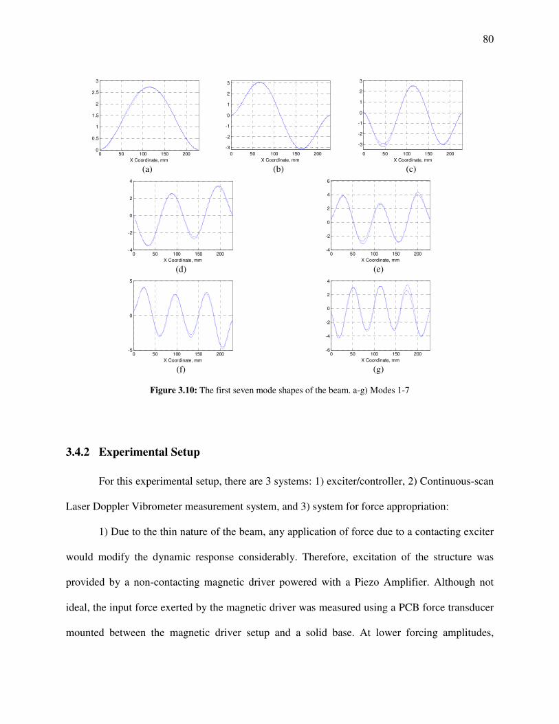
80

0 50 100 150 2000

0.5

1

1.5

2

2.5

3

X Coordinate, mm (a)

0 50 100 150 200

-3

-2

-1

0

1

2

3

X Coordinate, mm (b)

0 50 100 150 200

-3

-2

-1

0

1

2

3

X Coordinate, mm (c)

0 50 100 150 200-4

-2

0

2

4

X Coordinate, mm (d)

0 50 100 150 200-4

-2

0

2

4

6

X Coordinate, mm (e)

0 50 100 150 200-5

0

5

X Coordinate, mm (f)

0 50 100 150 200-6

-4

-2

0

2

4

X Coordinate, mm (g)

Figure 3.10: The first seven mode shapes of the beam. a-g) Modes 1-7

3.4.2 Experimental Setup

For this experimental setup, there are 3 systems: 1) exciter/controller, 2) Continuous-scan

Laser Doppler Vibrometer measurement system, and 3) system for force appropriation:

1) Due to the thin nature of the beam, any application of force due to a contacting exciter

would modify the dynamic response considerably. Therefore, excitation of the structure was

provided by a non-contacting magnetic driver powered with a Piezo Amplifier. Although not

ideal, the input force exerted by the magnetic driver was measured using a PCB force transducer

mounted between the magnetic driver setup and a solid base. At lower forcing amplitudes,

81

complementary results between the input voltage and measured force were found but showed a

small phase difference. At higher forcing amplitudes, the magnetic driver setup further

contaminated the measured force as discussed in the results section. At low and high forcing

amplitudes the response of the beam follows the input voltage building confidence in the use of

the voltage signal as the input force level.

2) Full-field dynamic measurements were taken using Continuous-scan laser Doppler

vibrometry (CSLDV) and full-static measurements were taken using three dimensional digital

image correlation (3D-DIC). Details for both of these measurement techniques can be found

[42]. 3D-DIC will be used to determine any initial curvature of the structure and CSLDV will be

used to determine the LNMs participating in the nonlinear response.

3) Prior to scanning the single point laser Doppler vibrometer (LDV) was used to

measure the response of the beam as it was subjected to a single frequency sinusoid at a specified

excitation amplitude. The voltage input to the exciter was measured as well as the input force for

the magnetic driver and the base acceleration for the shaker. The velocity response and input

voltage signals were measured in real time and displayed in a built LabView program capable of

modifying the amplitude and frequency distribution of the external force being input to the beam.

Here, the input voltage was used instead of the measured force to limit noise contamination from

the measurement sensors. The input frequency and amplitude distribution could then be

determined by adjusting the frequency of the fundamental harmonic and amplitudes of the input

harmonics until the input voltage and response velocity traced a line (e.g. the area enclosed by

the curve was zero). In a post processing step, the phase relationship for all harmonics was

examined more precisely.

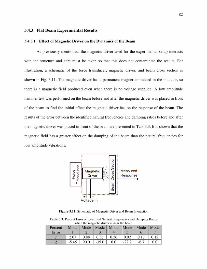
82

3.4.3 Flat Beam Experimental Results

3.4.3.1 Effect of Magnetic Driver on the Dynamics of the Beam

As previously mentioned, the magnetic driver used for the experimental setup interacts

with the structure and care must be taken so that this does not contaminate the results. For

illustration, a schematic of the force transducer, magnetic driver, and beam cross section is

shown in Fig. 3.11. The magnetic driver has a permanent magnet embedded in the inductor, so

there is a magnetic field produced even when there is no voltage supplied. A low amplitude

hammer test was performed on the beam before and after the magnetic driver was placed in front

of the beam to find the initial effect the magnetic driver has on the response of the beam. The

results of the error between the identified natural frequencies and damping ratios before and after

the magnetic driver was placed in front of the beam are presented in Tab. 3.3. It is shown that the

magnetic field has a greater effect on the damping of the beam than the natural frequencies for

low amplitude vibrations.

Figure 3.11: Schematic of Magnetic Driver and Beam Interaction

Table 3.3: Percent Error of Identified Natural Frequencies and Damping Ratios

when the magnetic driver is near the beam

Percent

Error

Mode

1

Mode

2

Mode

3

Mode

4

Mode

5

Mode

6

Mode

7

f 2.07 0.88 0.36 0.26 0.02 0.17 0.12

ξ -5.45 90.0 -35.0 0.0 -22.2 -6.7 0.0

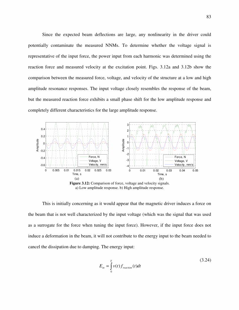
83

Since the expected beam deflections are large, any nonlinearity in the driver could

potentially contaminate the measured NNMs. To determine whether the voltage signal is

representative of the input force, the power input from each harmonic was determined using the

reaction force and measured velocity at the excitation point. Figs. 3.12a and 3.12b show the

comparison between the measured force, voltage, and velocity of the structure at a low and high

amplitude resonance responses. The input voltage closely resembles the response of the beam,

but the measured reaction force exhibits a small phase shift for the low amplitude response and

completely different characteristics for the large amplitude response.

0 0.005 0.01 0.015 0.02 0.025 0.03

-0.6

-0.4

-0.2

0

0.2

0.4

Time, s

Am

plitu

de

Force, N

Voltage, V

Velocity, mm/s

(a)

0 0.01 0.02 0.03 0.04 0.05

-4

-3

-2

-1

0

1

2

3

Time, s

Am

plitu

de

Force, N

Voltage, V

Velocity, mm/s

(b)

Figure 3.12: Comparison of force, voltage and velocity signals.

a) Low amplitude response. b) High amplitude response.

This is initially concerning as it would appear that the magnetic driver induces a force on

the beam that is not well characterized by the input voltage (which was the signal that was used

as a surrogate for the force when tuning the input force). However, if the input force does not

induce a deformation in the beam, it will not contribute to the energy input to the beam needed to

cancel the dissipation due to damping. The energy input:

dttftvE

T

reactionin ∫=0

)()(

(3.24)

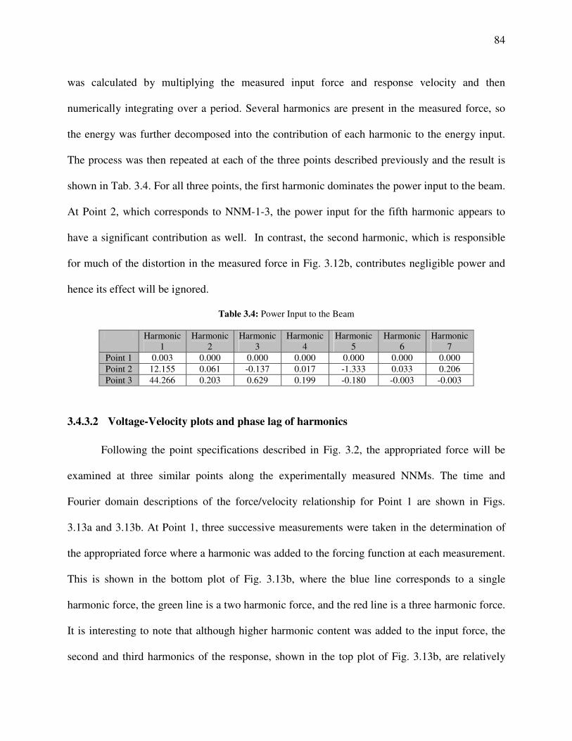
84

was calculated by multiplying the measured input force and response velocity and then

numerically integrating over a period. Several harmonics are present in the measured force, so

the energy was further decomposed into the contribution of each harmonic to the energy input.

The process was then repeated at each of the three points described previously and the result is

shown in Tab. 3.4. For all three points, the first harmonic dominates the power input to the beam.

At Point 2, which corresponds to NNM-1-3, the power input for the fifth harmonic appears to

have a significant contribution as well. In contrast, the second harmonic, which is responsible

for much of the distortion in the measured force in Fig. 3.12b, contributes negligible power and

hence its effect will be ignored.

Table 3.4: Power Input to the Beam

Harmonic

1

Harmonic

2

Harmonic

3

Harmonic

4

Harmonic

5

Harmonic

6

Harmonic

7

Point 1 0.003 0.000 0.000 0.000 0.000 0.000 0.000

Point 2 12.155 0.061 -0.137 0.017 -1.333 0.033 0.206

Point 3 44.266 0.203 0.629 0.199 -0.180 -0.003 -0.003

3.4.3.2 Voltage-Velocity plots and phase lag of harmonics

Following the point specifications described in Fig. 3.2, the appropriated force will be

examined at three similar points along the experimentally measured NNMs. The time and

Fourier domain descriptions of the force/velocity relationship for Point 1 are shown in Figs.

3.13a and 3.13b. At Point 1, three successive measurements were taken in the determination of

the appropriated force where a harmonic was added to the forcing function at each measurement.

This is shown in the bottom plot of Fig. 3.13b, where the blue line corresponds to a single

harmonic force, the green line is a two harmonic force, and the red line is a three harmonic force.

It is interesting to note that although higher harmonic content was added to the input force, the

second and third harmonics of the response, shown in the top plot of Fig. 3.13b, are relatively

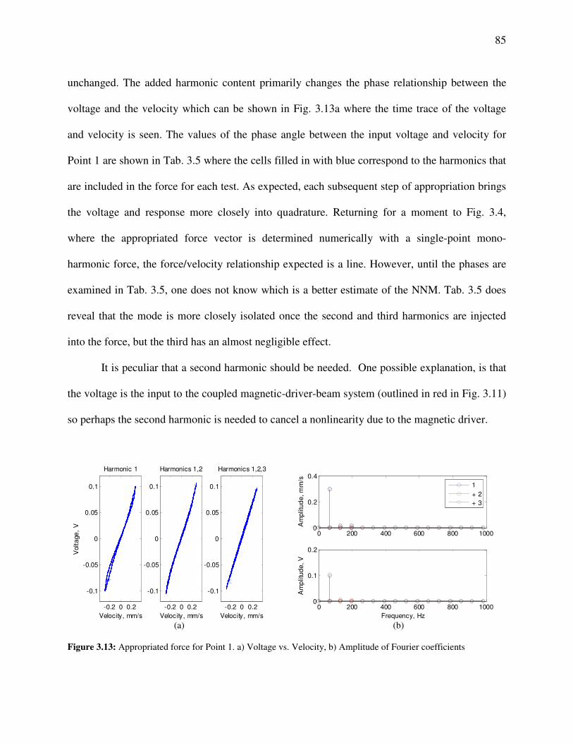
85

unchanged. The added harmonic content primarily changes the phase relationship between the

voltage and the velocity which can be shown in Fig. 3.13a where the time trace of the voltage

and velocity is seen. The values of the phase angle between the input voltage and velocity for

Point 1 are shown in Tab. 3.5 where the cells filled in with blue correspond to the harmonics that

are included in the force for each test. As expected, each subsequent step of appropriation brings

the voltage and response more closely into quadrature. Returning for a moment to Fig. 3.4,

where the appropriated force vector is determined numerically with a single-point mono-

harmonic force, the force/velocity relationship expected is a line. However, until the phases are

examined in Tab. 3.5, one does not know which is a better estimate of the NNM. Tab. 3.5 does

reveal that the mode is more closely isolated once the second and third harmonics are injected

into the force, but the third has an almost negligible effect.

It is peculiar that a second harmonic should be needed. One possible explanation, is that

the voltage is the input to the coupled magnetic-driver-beam system (outlined in red in Fig. 3.11)

so perhaps the second harmonic is needed to cancel a nonlinearity due to the magnetic driver.

-0.2 0 0.2

-0.1

-0.05

0

0.05

0.1

Harmonic 1

Velocity, mm/s

Volt

age

, V

-0.2 0 0.2

-0.1

-0.05

0

0.05

0.1

Velocity, mm/s

Harmonics 1,2

-0.2 0 0.2

-0.1

-0.05

0

0.05

0.1

Velocity, mm/s

Harmonics 1,2,3

(a)

0 200 400 600 800 10000

0.2

0.4

Am

plitu

de

, m

m/s

0 200 400 600 800 10000

0.1

0.2

Frequency, Hz

Am

plitu

de

, V

1

+ 2

+ 3

(b)

Figure 3.13: Appropriated force for Point 1. a) Voltage vs. Velocity, b) Amplitude of Fourier coefficients

86

This process is repeated for Points 2 and 3. Again, converging values of the phase are

observed between the voltage and velocity as higher harmonics are added to the input voltage. It

should be noted that since Point 2 (Fig. 3.14) and Point 3 (Fig. 3.15) correspond to a greater

nonlinear behavior of the beam, more harmonic content is needed to cancel the damping

observed. In the tests performed, the harmonics were tuned in an effort to minimize the enclosed

area in the curve. In the appropriated response for Point 2, Fig. 3.14, the voltage/velocity

relationship indicates that as higher harmonics are added, the shape of the voltage/velocity plot

changes providing insight to how each added harmonic changes the response. When compared

with the numerically calculated force/velocity relationship, Fig. 3.5, the force characteristics that

that includes only the first and fifth harmonics best matches the appropriated response indicating

the best experimental force distribution. Similarly, the voltage/velocity relationship observed for

Point 3 (Fig. 3.15) indicates that the force that includes only the first and third harmonic better

matches the numerically determined force/velocity relationship established in Fig. 3.6.

-0.5 0 0.5-0.4

-0.2

0

0.2

0.4Harmonic 1

Volt

age

, V

-0.5 0 0.5-0.4

-0.2

0

0.2

0.4

Volt

age

, V

Harmonics 1,5

-0.5 0 0.5-0.4

-0.2

0

0.2

0.4

Velocity, mm/s

Volta

ge

, V

Harmonics 1,5,7

-0.5 0 0.5-0.4

-0.2

0

0.2

0.4

Velocity, mm/s

Volta

ge

, V

Harmonics 1,3,5,7

(a)

0 500 1000 15000

0.2

0.4

0.6

0.8

Am

plitu

de

, m

m/s

0 500 1000 15000

0.1

0.2

0.3

0.4

Frequency, Hz

Am

plitu

de

, V

1

+ 5

+ 7

+ 3

(b)

Figure 3.14: Appropriated force for Point 2. a) Voltage vs. Velocity, b) Amplitude of Fourier coefficients

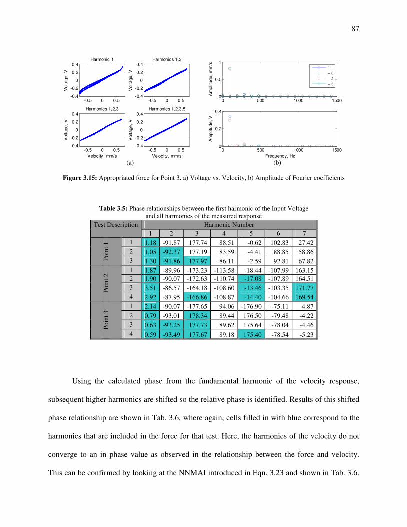
87

-0.5 0 0.5-0.4

-0.2

0

0.2

0.4Harmonic 1

Volt

age

, V

-0.5 0 0.5-0.4

-0.2

0

0.2

0.4

Volt

age

, V

Harmonics 1,3

-0.5 0 0.5-0.4

-0.2

0

0.2

0.4

Velocity, mm/s

Volt

age

, V

Harmonics 1,2,3

-0.5 0 0.5-0.4

-0.2

0

0.2

0.4

Velocity, mm/s

Volt

age

, V

Harmonics 1,2,3,5

(a)

0 500 1000 15000

0.5

1

Am

plitu

de

, m

m/s

0 500 1000 15000

0.2

0.4

Frequency, Hz

Am

plitu

de

, V

1

+ 3

+ 2

+ 5

(b)

Figure 3.15: Appropriated force for Point 3. a) Voltage vs. Velocity, b) Amplitude of Fourier coefficients

Table 3.5: Phase relationships between the first harmonic of the Input Voltage

and all harmonics of the measured response

Harmonic Number Test Description

1 2 3 4 5 6 7

1 1.18 -91.87 177.74 88.51 -0.62 102.83 27.42

2 1.05 -92.37 177.19 83.59 -4.41 88.85 58.86

Po

int

1

3 1.30 -91.86 177.97 86.11 -2.59 92.81 67.82

1 1.87 -89.96 -173.23 -113.58 -18.44 -107.99 163.15

2 1.90 -90.07 -172.63 -110.74 -17.08 -107.89 164.51

3 3.51 -86.57 -164.18 -108.60 -13.46 -103.35 171.77 Po

int

2

4 2.92 -87.95 -166.86 -108.87 -14.40 -104.66 169.54

1 2.14 -90.07 -177.65 94.06 -176.90 -75.11 4.87

2 0.79 -93.01 178.34 89.44 176.50 -79.48 -4.22

3 0.63 -93.25 177.73 89.62 175.64 -78.04 -4.46 Po

int

3

4 0.59 -93.49 177.67 89.18 175.40 -78.54 -5.23

Using the calculated phase from the fundamental harmonic of the velocity response,

subsequent higher harmonics are shifted so the relative phase is identified. Results of this shifted

phase relationship are shown in Tab. 3.6, where again, cells filled in with blue correspond to the

harmonics that are included in the force for that test. Here, the harmonics of the velocity do not

converge to an in phase value as observed in the relationship between the force and velocity.

This can be confirmed by looking at the NNMAI introduced in Eqn. 3.23 and shown in Tab. 3.6.

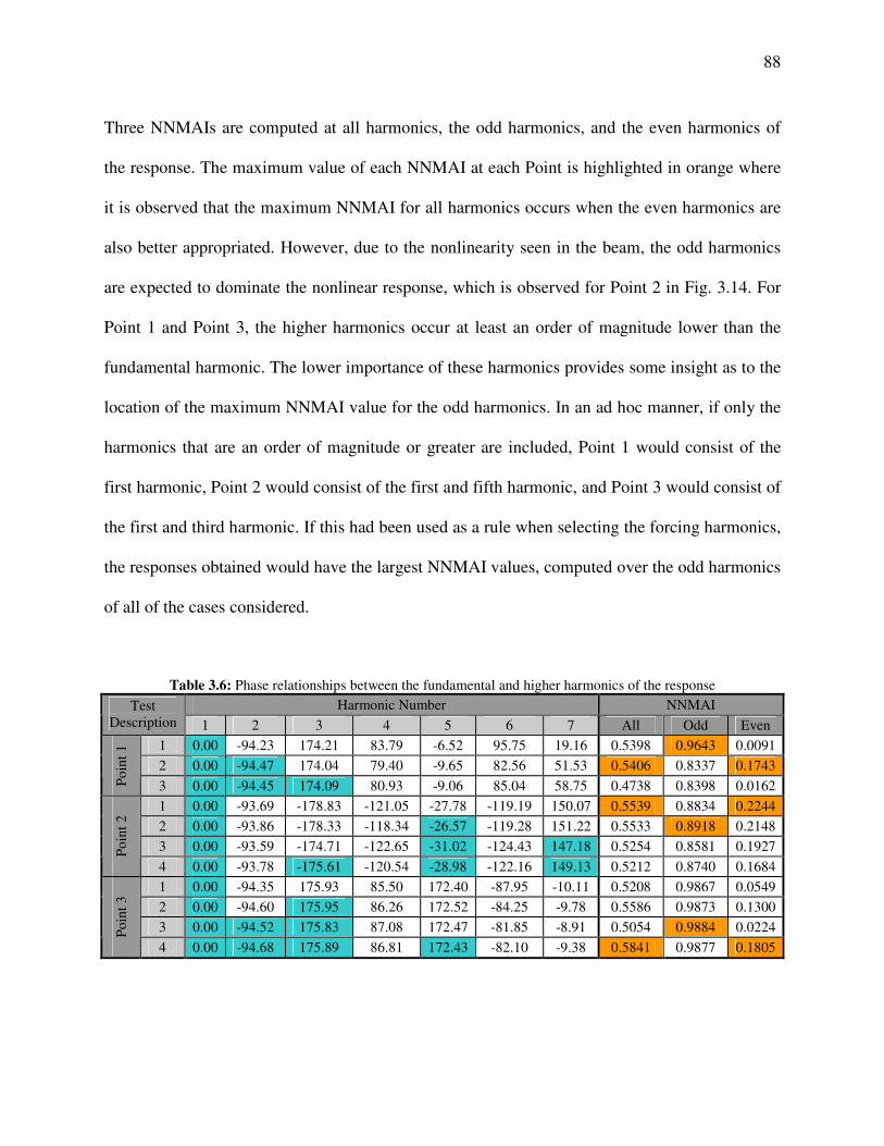
88

Three NNMAIs are computed at all harmonics, the odd harmonics, and the even harmonics of

the response. The maximum value of each NNMAI at each Point is highlighted in orange where

it is observed that the maximum NNMAI for all harmonics occurs when the even harmonics are

also better appropriated. However, due to the nonlinearity seen in the beam, the odd harmonics

are expected to dominate the nonlinear response, which is observed for Point 2 in Fig. 3.14. For

Point 1 and Point 3, the higher harmonics occur at least an order of magnitude lower than the

fundamental harmonic. The lower importance of these harmonics provides some insight as to the

location of the maximum NNMAI value for the odd harmonics. In an ad hoc manner, if only the

harmonics that are an order of magnitude or greater are included, Point 1 would consist of the

first harmonic, Point 2 would consist of the first and fifth harmonic, and Point 3 would consist of

the first and third harmonic. If this had been used as a rule when selecting the forcing harmonics,

the responses obtained would have the largest NNMAI values, computed over the odd harmonics

of all of the cases considered.

Table 3.6: Phase relationships between the fundamental and higher harmonics of the response

Harmonic Number NNMAI Test

Description 1 2 3 4 5 6 7 All Odd Even

1 0.00 -94.23 174.21 83.79 -6.52 95.75 19.16 0.5398 0.9643 0.0091

2 0.00 -94.47 174.04 79.40 -9.65 82.56 51.53 0.5406 0.8337 0.1743

Po

int

1

3 0.00 -94.45 174.09 80.93 -9.06 85.04 58.75 0.4738 0.8398 0.0162

1 0.00 -93.69 -178.83 -121.05 -27.78 -119.19 150.07 0.5539 0.8834 0.2244

2 0.00 -93.86 -178.33 -118.34 -26.57 -119.28 151.22 0.5533 0.8918 0.2148

3 0.00 -93.59 -174.71 -122.65 -31.02 -124.43 147.18 0.5254 0.8581 0.1927 Po

int

2

4 0.00 -93.78 -175.61 -120.54 -28.98 -122.16 149.13 0.5212 0.8740 0.1684

1 0.00 -94.35 175.93 85.50 172.40 -87.95 -10.11 0.5208 0.9867 0.0549

2 0.00 -94.60 175.95 86.26 172.52 -84.25 -9.78 0.5586 0.9873 0.1300

3 0.00 -94.52 175.83 87.08 172.47 -81.85 -8.91 0.5054 0.9884 0.0224 Po

int

3

4 0.00 -94.68 175.89 86.81 172.43 -82.10 -9.38 0.5841 0.9877 0.1805

89

For any of the selected force distributions, the odd harmonics can be considered well

appropriated (e.g. all NNMAI values are above 0.83) and this confirms that the stepped-sine

backbone is well appropriated if the structure is governed only by the odd harmonics. If all

harmonics are considered, NNMAI values greater than 0.5 are obtained for the appropriated

responses still provides a well appropriated NNM when compared with simulation results .

3.4.3.3 Experimental Frequency-Amplitude Results

The two NNMs previously discussed were isolated in an experiment using the previously

described techniques. As discussed previously, the appropriation was probably not perfect, but

seems to be as accurate as possible given the limitations of the experimental setup. Before

examining the NNMs, it is beneficial to examine the two time series decays and their

corresponding Morlet wavelet transform coefficients, shown in Fig. 3.16. For reference, the two

decays were initiated near the previously described Point 2 and Point 3 shown in Figs. 3.5 and

3.6. Figures 3.16a and 3.16b are the time series and wavelet transform results from the Point 3

decay measured with the single point LDV at the center of the beam. The decay is initiated at

106.98 Hz, consequent of a 61.18 Hz shift in the first mode of the beam, and is expected to

tracks the NNM backbone through the bifurcation of the backbone to the IR. There is a bump in

the time series and in the amplitude vs. time of the fifth harmonic from the wavelet near 2.5

seconds. It will be shown later that this occurs near the 5:1 internal resonance on NNM-1.

Figures 3.16c and 3.16d show the time series and wavelet transform results from the

decay from Point 2 with the same experimental setup. Although the decay is initiated at only

82.60 Hz, consequent of a 36.80 Hz shift in the first mode of the beam, the peak amplitude of the

90

time response prior to the decay is near that of the Point 3 decay shown in Fig. 3.16a. This can be

related to the numeric results previously presented where periodic solutions can occur at two

different fundamental frequencies and the same energy levels, only here this is observed in terms

of peak amplitude instead of energy. For the decay of Point 2, wavelet coefficients at the 5th

harmonic are on a similar scale as the fundamental harmonic as seen in Fig. 3.16d. This can be

related to a larger amount of energy being transferred to the 5:1 IR NNSPS, so this harmonic will

need to be included in the reconstruction of the NNM.

Similarly, a decay experiment was performed on NNM-3. Only one decay experiment is

needed since no coupling was predicted in the numerical model of NNM-3. This is confirmed by

examining the wavelet transform shown in Fig. 3.16f where no coupling with higher modes is

present. A small but interesting "coupling" occurs with LNM-1, which can be seen near the

bottom of the plot in light blue. This "coupling" only occurs once the force has been turned off

and does not see any change in frequency throughout the decay. Therefore, it was concluded that

the observed "coupling" is most likely a result of how the force was removed for the decay,

which was not always at the static equilibrium point of the deformation of the beam, and not a

true indication of nonlinear coupling in the beam. Additionally, since NNM-3 occurs at a higher

frequency, the response decays in a third of the time required for NNM-1 to decay. This is a well

defined occurrence in structural dynamics, but is repeated here as it can affect the ability of the

wavelet transform to detect higher harmonics of the response if the sampling frequency and

length of time recorded are not sufficiently large.

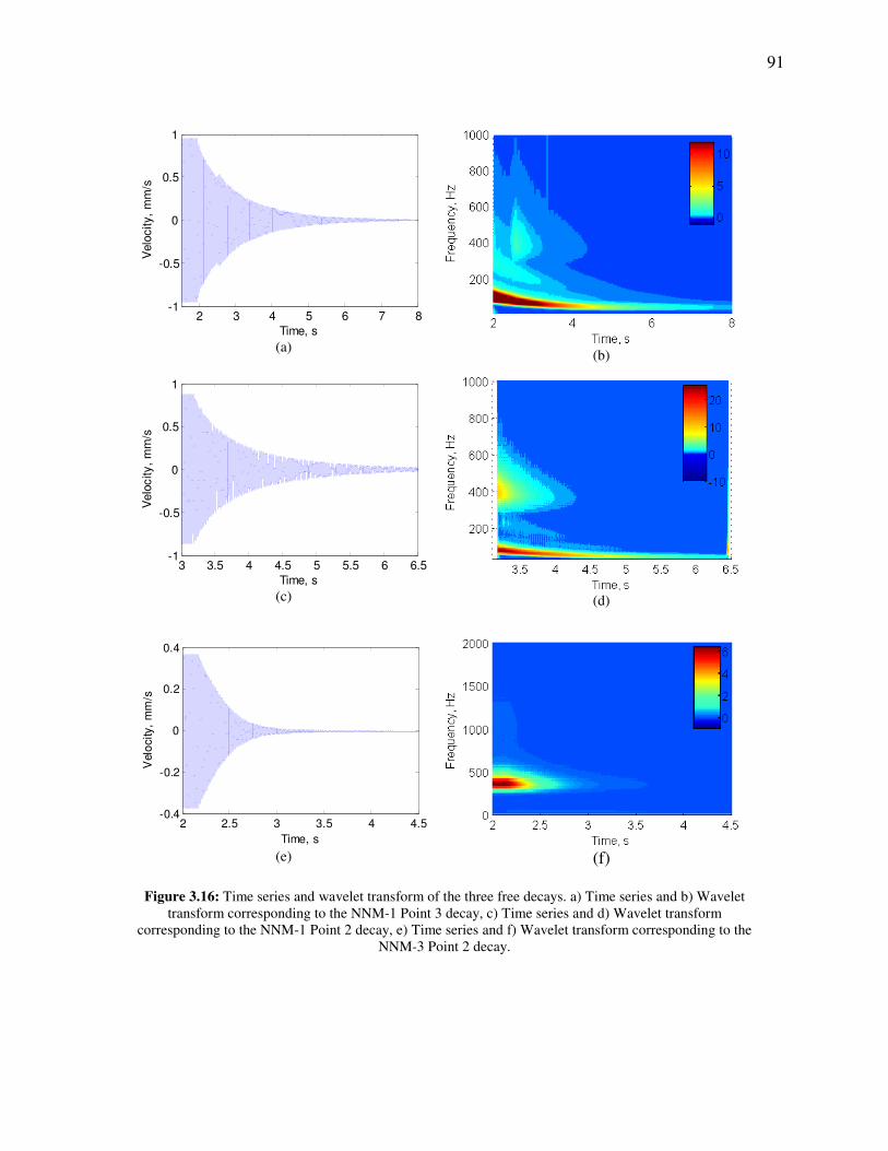
91

2 3 4 5 6 7 8-1

-0.5

0

0.5

1

Time, s

Velo

city,

mm

/s

(a)

(b)

3 3.5 4 4.5 5 5.5 6 6.5-1

-0.5

0

0.5

1

Time, s

Velo

city,

mm

/s

(c)

(d)

2 2.5 3 3.5 4 4.5-0.4

-0.2

0

0.2

0.4

Time, s

Velo

city,

mm

/s

(e)

(f)

Figure 3.16: Time series and wavelet transform of the three free decays. a) Time series and b) Wavelet

transform corresponding to the NNM-1 Point 3 decay, c) Time series and d) Wavelet transform

corresponding to the NNM-1 Point 2 decay, e) Time series and f) Wavelet transform corresponding to the

NNM-3 Point 2 decay.

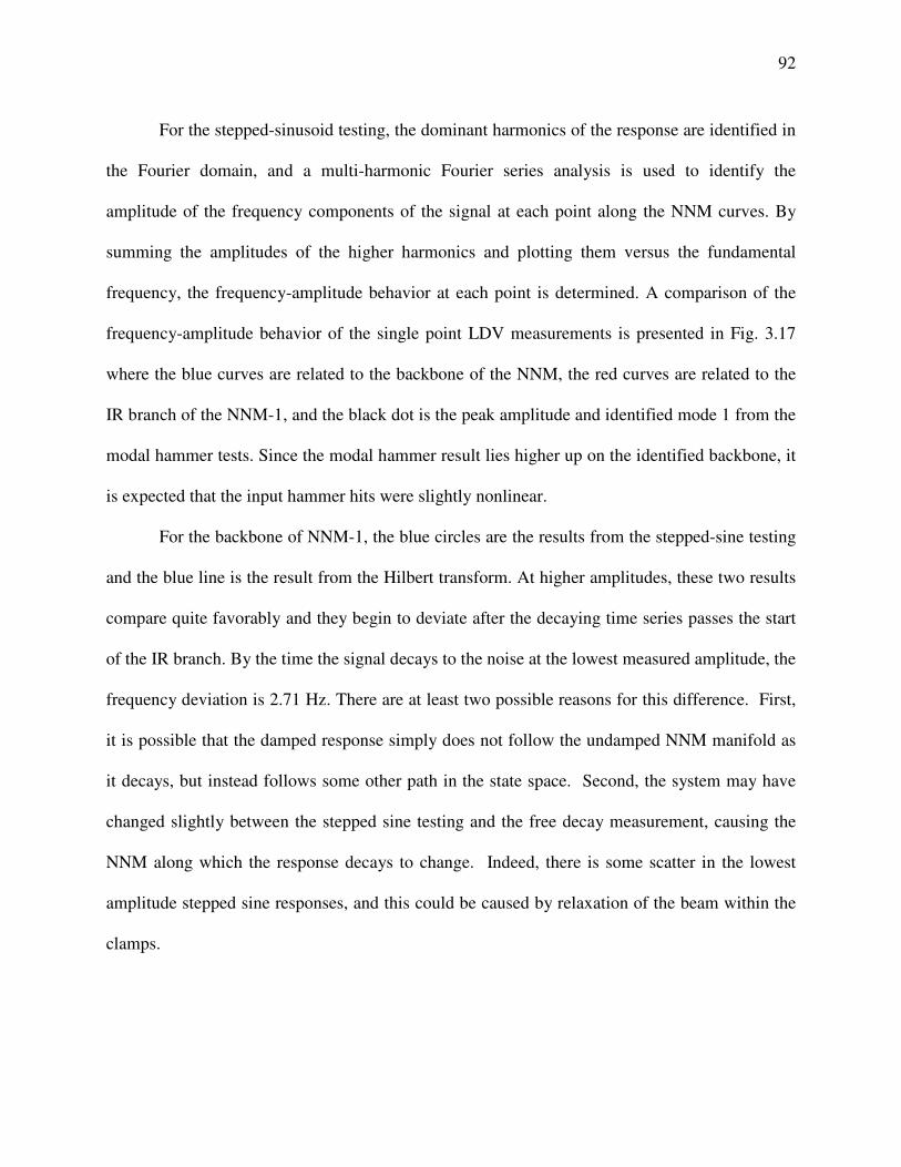
92

For the stepped-sinusoid testing, the dominant harmonics of the response are identified in

the Fourier domain, and a multi-harmonic Fourier series analysis is used to identify the

amplitude of the frequency components of the signal at each point along the NNM curves. By

summing the amplitudes of the higher harmonics and plotting them versus the fundamental

frequency, the frequency-amplitude behavior at each point is determined. A comparison of the

frequency-amplitude behavior of the single point LDV measurements is presented in Fig. 3.17

where the blue curves are related to the backbone of the NNM, the red curves are related to the

IR branch of the NNM-1, and the black dot is the peak amplitude and identified mode 1 from the

modal hammer tests. Since the modal hammer result lies higher up on the identified backbone, it

is expected that the input hammer hits were slightly nonlinear.

For the backbone of NNM-1, the blue circles are the results from the stepped-sine testing

and the blue line is the result from the Hilbert transform. At higher amplitudes, these two results

compare quite favorably and they begin to deviate after the decaying time series passes the start

of the IR branch. By the time the signal decays to the noise at the lowest measured amplitude, the

frequency deviation is 2.71 Hz. There are at least two possible reasons for this difference. First,

it is possible that the damped response simply does not follow the undamped NNM manifold as

it decays, but instead follows some other path in the state space. Second, the system may have

changed slightly between the stepped sine testing and the free decay measurement, causing the

NNM along which the response decays to change. Indeed, there is some scatter in the lowest

amplitude stepped sine responses, and this could be caused by relaxation of the beam within the

clamps.

93

When comparing the free decay that started near the IR branch, in red, we see a larger

deviation between the path followed by the free decay and the NNM. Although somewhat

scattered at higher amplitudes, the stepped-sine measurements appear to capture the point of

bifurcation from the backbone well and to follow up the internal resonance. This is not the case

when looking at the free decay from the IR branch. The amplitude of the decaying signal has a

significantly higher amplitude than the NNM estimated from the stepped-sine measurements,

until the amplitude becomes low and the two curves converge. Interestingly, this free response

tracks the measured stepped-sine NNM better than the free response that was initiated on the

stepped sine backbone.

There are several possible explanations as to why this is could occur. First, it should be

noted that the appropriated force was at a lower quality on the IR branch than on the backbone

which could explain why the NNM was not as closely followed. Second, since the IR branch

involves an interaction between two NNMs, it could be that the decaying response is being

pulled between two attractors and hence not following either NNM precisely.

40 50 60 70 80 90 100 110

10-2

10-1

100

Frequency, Hz

Max A

mp

litud

e o

f V

elo

cit

y, m

m/s

Backbone, Stepped Sine

Backbone, Free Decay

IR, Stepped Sine

IR, Free Decay

Hammer

40 50 60 70 80 90 100 110

2

4

6

8

Tim

e C

orr

esp

ond

ing

to t

he F

ree D

eca

y, s

40 50 60 70 80 90 100 110

4

5

6

7

Figure 3.17: Frequency-Amplitude behavior of NNM-1 and NNM-1-3

94

A similar comparison can be made between the stepped sine and free decay experiments

performed on NNM-3, shown in Fig. 3.18. The maximum percent error between the free decay

and stepped-sine methods is 0.95%. Again, there is an offset between the free decays results and

the stepped sine estimated NNM, but there was also a difference in the frequency between the

linear hammer test and the stepped-sine results of 1.5%, so once again it is possible that the

boundary conditions changed from one test to the next.

364 366 368 370 372 374 376 378 380 38210

-3

10-2

10-1

100

Frequency, Hz

Max A

mp

litude o

f V

elo

city, m

m/s

Backbone, Stepped Sine

Backbone, Free Decay

Hammer

364 366 368 370 372 374 376 378 380 382

2

2.5

3

3.5

4

4.5 Tim

e C

orr

esp

ond

ing t

o t

he F

ree

Deacy,

s

Figure 3.18: Frequency-Amplitude behavior of NNM-3

3.4.3.4 Full-Field Deformation Shapes

Another benefit to the use of stepped-sine testing is the ability to use advanced full-field

measurement techniques effectively. As seen with the numerical results, the examination of the

deformation shapes along the NNM for the beam provides insight to how the LNMs of the

structure couple. Due to the relatively small deformation expected in the beam, continuous-scan

laser Doppler vibrometry (CSLDV) is used to measure the surface using a line scan pattern as

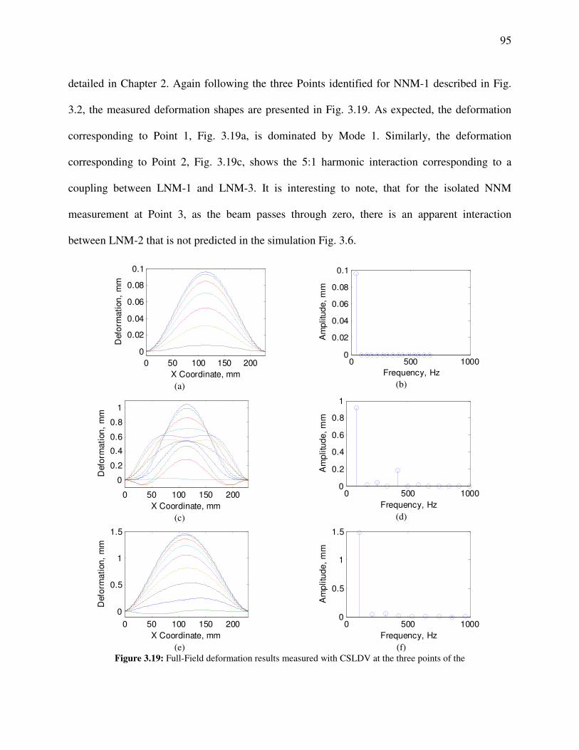
95

detailed in Chapter 2. Again following the three Points identified for NNM-1 described in Fig.

3.2, the measured deformation shapes are presented in Fig. 3.19. As expected, the deformation

corresponding to Point 1, Fig. 3.19a, is dominated by Mode 1. Similarly, the deformation

corresponding to Point 2, Fig. 3.19c, shows the 5:1 harmonic interaction corresponding to a

coupling between LNM-1 and LNM-3. It is interesting to note, that for the isolated NNM

measurement at Point 3, as the beam passes through zero, there is an apparent interaction

between LNM-2 that is not predicted in the simulation Fig. 3.6.

0 50 100 150 200

0

0.02

0.04

0.06

0.08

0.1

X Coordinate, mm

Defo

rmati

on

, m

m

(a)

0 500 10000

0.02

0.04

0.06

0.08

0.1

Frequency, Hz

Am

plitu

de, m

m

(b)

0 50 100 150 200

0

0.2

0.4

0.6

0.8

1

X Coordinate, mm

Defo

rmati

on

, m

m

(c)

0 500 10000

0.2

0.4

0.6

0.8

1

Frequency, Hz

Am

plitu

de

, m

m

(d)

0 50 100 150 200

0

0.5

1

1.5

X Coordinate, mm

Defo

rma

tion

, m

m

(e)

0 500 10000

0.5

1

1.5

Frequency, Hz

Am

plitu

de

, m

m

(f)

Figure 3.19: Full-Field deformation results measured with CSLDV at the three points of the

96

A further decomposition of the harmonics of the response and projection onto the LNMs

further identify the nonlinear coupling between the LNMs. For nonlinear systems, the

measurement of the deformation shapes at each harmonic also provides insight and these shapes

can then be projected onto the LNMs to understand where they come from and perhaps even

create a nonlinear reduced order model (NLROM) with the LNMs as a basis (as discussed in

Chapter Error! Reference source not found.: Future Work).

3.5 Application to Axi-symmetric Curved Plate with Geometric Nonlinearity

3.5.1 Plate Description

The second article under investigation is a circular perforated plate with rolled ends

which is shown in Fig. 3.20. A mechanical punch was used to create the circular perforations in a

flat 16 gauge (1.52 mm thick) 409 stainless steel plate in an array of equilateral triangles with

10.16 mm long edges. Once this process was completed, the plate was formed around a 317.5

mm diameter mold with the excess trimmed so a lip of 12 mm remained. The plate was then

welded to a 89 mm high cylinder made from a 14 gauge (1.9 mm thick) 409 stainless steel plate

that was cold rolled to the 317.5 mm diameter. The welded plate assembly was then bolted to a

317.5 mm diameter by 19 mm thick aluminum fixture with twelve 6.4 mm evenly spaced holes.

Due to the relatively complex processes used to create this test piece, it is important to note that

all stated dimensions are nominal and subject to variation. Additionally, the processes the plate is

subjected to can induce residual stresses in the structure which also might modify the dynamics

of the plate in its final configuration and are not considered here.

97

CSLDV was not used in this experiment due to the discontinuities from the perforations.

Instead the surface was prepared for high speed 3D-DIC, as shown in Fig. 3.20. 3D-DIC was

able to provide the full-field measurements of the plate since there was enough room between the

perforations to capture surface deformations. Additionally, Fig. 3.20 also shows the location of

the single point laser Doppler vibrometers (LDV). After mounting, a single-input single-output

modal hammer test was performed on the plate so natural frequencies and damping ratios could

be identified. Results for the first nine modes are shown in Tab. 3.7. A linear mode shape

comparison between a roving hammer test and the nominal model for the first six identified

modes is shown in Fig. 3.21.

Figure 3.20: Final Mounted Perforated Plate

Table 3.7: Linear (low amplitude) natural frequencies of curved axi-symmetric plate

Mode 1 Mode 2 Mode 3 Mode 4 Mode 5 Mode 6 Mode 7 Mode 8 Mode 9

f, Hz 202.2 324 342.8 489.7 509.9 554.1 697.2 777.9 794.2

ζ1 , % 0.2 0.13 0.31 0.092 0.15 0.087 0.11 0.49 0.43

98

(a)

(b)

(c)

(d)

(e)

(f)

Figure 3.21: First six mode shapes for the Nominally Flat Model compared with a roving hammer

test

While this system is relatively simple compared to the engine to which it is designed to

be attached, the nominal model provides relatively large number of DOF than structures

previously investigated in this dissertation. Since the previously discussed NNM analysis

techniques have been focused on low DOF systems, a nonlinear reduced order model (NLROM)

99

is needed to determine the numerical NNMs of the structure. This can potentially lead to a

variety of subtle details that might easily be neglected initially, and yet they could change the

response considerably. Therefore, there is a greater reliance on experimental techniques in this

case that can readily identify any nonlinear coupling that can occur between the LNMs. In this

context, the use of full-field measurement techniques provides the information needed to confirm

the NLROM captures the nonlinear behavior well.

3.5.2 Plate NNM Calculation

Fig. 3.22a shows the NNM-1 FEP for the curved axi-symmetric plate with an added line

denoting 1-thickness of deformation (e.g. 1.52mm for the plate). The numerically calculated

backbone was determined with a reduce-order model (ROM) where the continuation of the first

linear normal mode to higher energies was isolated. While this limits the ability to calculate

internal resonances in the plate, this one mode ROM still provides insight into the frequency-

energy dependence of NNM-1. As observed here, the NNM undergoes a change in the

characteristic nonlinearity as the fundamental frequency of vibration undergoes a decrease prior

to increasing. This softening to hardening characteristic can commonly be found in curved

structures [104, 105] and can be potentially damaging to the structure.

Similar to the flat beam, deformations of the curved axi-symmetric plate can also be

examined at points along the FEP to explore changes of the deformation shape due to the

increased response amplitudes. Since only mode 1 was used to calculate the NNM, Deformation

1 and 2, shown in Fig. 3.22b and Fig. 3.22c, are purely mode 1 shapes with different scale

factors. The effect of higher modes on an initially flat axi-symmetry plate was examined

numerically in [85] providing insight to the dynamics of an axi-symmetric plate, even though the

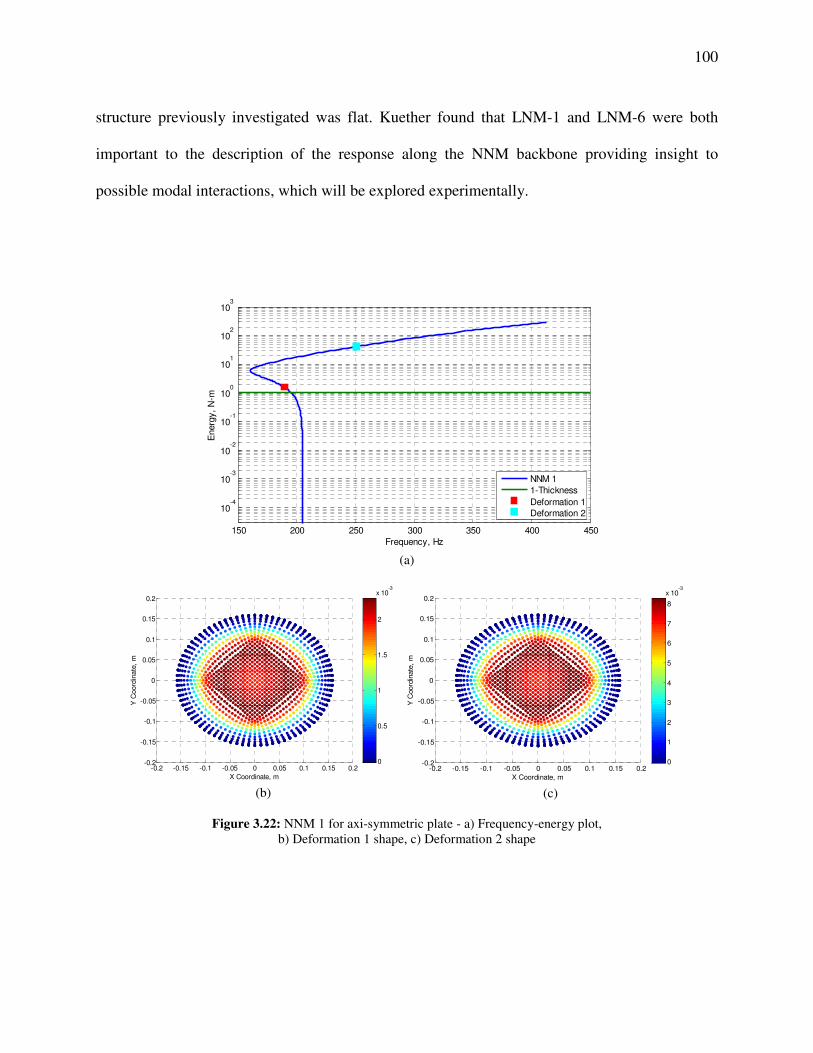
100

structure previously investigated was flat. Kuether found that LNM-1 and LNM-6 were both

important to the description of the response along the NNM backbone providing insight to

possible modal interactions, which will be explored experimentally.

150 200 250 300 350 400 450

10-4

10-3

10-2

10-1

100

101

102

103

Frequency, Hz

Energ

y,

N-m

NNM 1

1-Thickness

Deformation 1

Deformation 2

(a)

-0.2 -0.15 -0.1 -0.05 0 0.05 0.1 0.15 0.2-0.2

-0.15

-0.1

-0.05

0

0.05

0.1

0.15

0.2

X Coordinate, m

Y C

oord

inate

, m

0

0.5

1

1.5

2

x 10-3

(b)

-0.2 -0.15 -0.1 -0.05 0 0.05 0.1 0.15 0.2-0.2

-0.15

-0.1

-0.05

0

0.05

0.1

0.15

0.2

X Coordinate, m

Y C

oord

inate

, m

0

1

2

3

4

5

6

7

8

x 10-3

(c)

Figure 3.22: NNM 1 for axi-symmetric plate - a) Frequency-energy plot,

b) Deformation 1 shape, c) Deformation 2 shape

101

3.5.3 Plate NNM Measurement

Following a similar methodology to that of the flat beam previously discussed, NNM-1

was experimentally measured for the curved axi-symmetric plate using 3D-DIC. Figure 3.23

shows the experimentally measured NNM of the curved axi-symmetric plate with the velocity

response measured at the LDV point located at the [x,y] coordinates of [0.01,-0.03]. Similar to

the numerically calculated NNM in 3.22a, the experimentally measured NNM shows the

characteristic spring softening to hardening effect or a decrease of the fundamental frequency of

vibration which begins to increase at a specific input force level. Unfortunately, limited data was

gathered on the structure in the linear region of response due to inadequate capabilities of the

shaker to obtain lower forcing amplitudes. Also, the plate cracked when a higher input force

amplitude was attempted, so further testing at low amplitudes was impossible. Failure initially

occurred at the [x,y] coordinates of [-0.01,-0.01] which can be identified in 3.23c and d. With the

use of high speed 3D-digital image correlation, maximum deformation shapes of the plate at low

and higher energy are shown in 3.23b-e. Figures 3.23b and c show the deformation shape at an

instant in time at the low energy point marked “deformation 1” in 3.23a. The deformation at this

frequency-energy point resembles mode 1 of a flat plate as expected in linear results. Figure

3.23d & e show the deformation shape at the high energy point, or deformation 2 also shown in

3.23a.

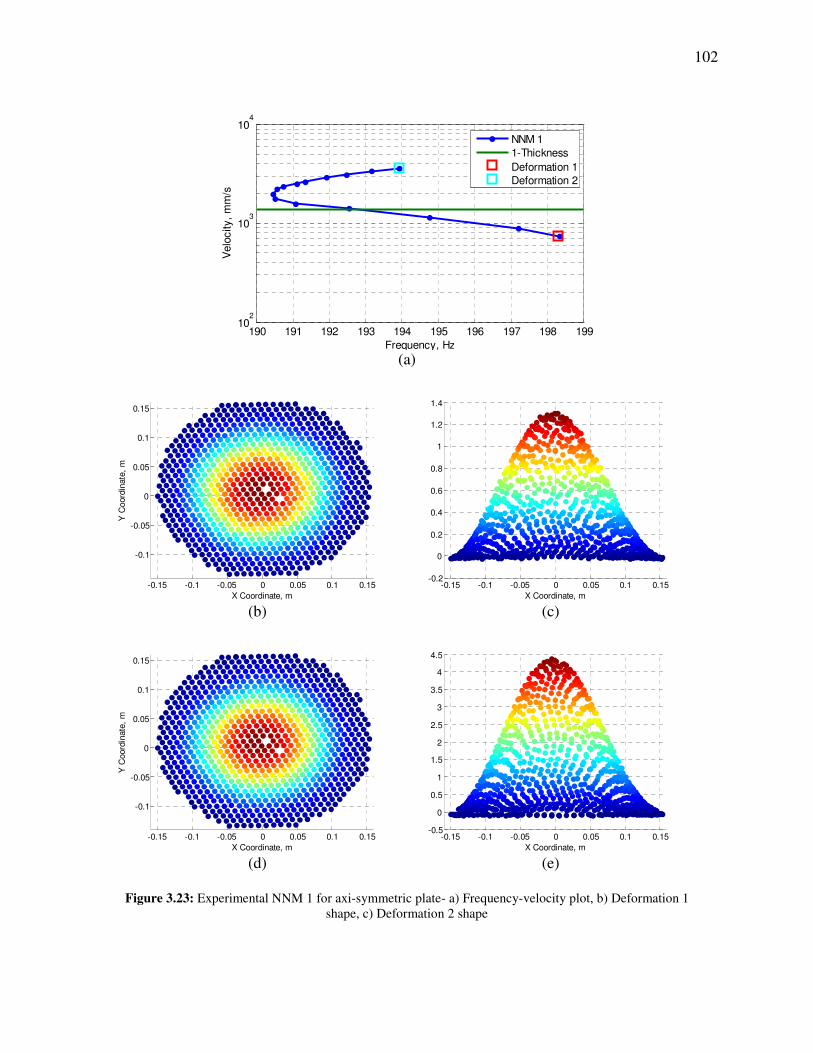
102

190 191 192 193 194 195 196 197 198 19910

2

103

104

Frequency, Hz

Velo

city,

mm

/s

NNM 1

1-Thickness

Deformation 1

Deformation 2

(a)

-0.15 -0.1 -0.05 0 0.05 0.1 0.15

-0.1

-0.05

0

0.05

0.1

0.15

X Coordinate, m

Y C

oord

inate

, m

(b)

-0.15 -0.1 -0.05 0 0.05 0.1 0.15-0.2

0

0.2

0.4

0.6

0.8

1

1.2

1.4

X Coordinate, m (c)

-0.15 -0.1 -0.05 0 0.05 0.1 0.15

-0.1

-0.05

0

0.05

0.1

0.15

X Coordinate, m

Y C

oord

inate

, m

(d)

-0.15 -0.1 -0.05 0 0.05 0.1 0.15-0.5

0

0.5

1

1.5

2

2.5

3

3.5

4

4.5

X Coordinate, m (e)

Figure 3.23: Experimental NNM 1 for axi-symmetric plate- a) Frequency-velocity plot, b) Deformation 1

shape, c) Deformation 2 shape

103

To obtain further insights, the measured response is decomposed into its harmonics in

Fig. 3.24a. Interestingly, this shows that while the fundamental harmonic is dominant at low

amplitude, as the response begins to turn from softening to hardening the higher harmonics

become large in the response. This is evident as the third harmonic of the measured velocity is

near equal to the first harmonic when the plate fails. Hence, while no internal resonances are

present the response of this NNM is multi-modal along the backbone. Unfortunately, the phase

of the harmonics, shown in 3.24b, reveal that the higher harmonics for the plate are not in

quadrature with the input force. So one cannot be sure that the NNM has been completely

isolated; however, since the excitation is mono-harmonic the phases of the higher harmonics

could be miss-leading since no force has been added. The first harmonic stays near 180 degrees

phase, but it is less accurate in the spring hardening regime, or on the lower amplitudes of the

response.

-4 -3.5 -3 -2.5 -2 -1.5 -1 -0.5 010

0

101

102

103

104

105

% Change in Frequency

Harm

on

ic A

mplitu

de

, m

m/s

1st Harmonic

2nd Harmonic

3rd Harmonic

4th Harmonic

5th Harmonic

(a)

-4 -3.5 -3 -2.5 -2 -1.5 -1 -0.5 0-180

-160

-140

-120

-100

-80

-60

-40

-20

0

% Change Frequency, -

Phase,

deg

1st Harmonic

2nd Harmonic

3rd Harmonic

4th Harmonic

5th Harmonic

(b)

Figure 3.24: NNM results for the axi-symmetric plate - a) FFT amplitude of harmonics in the response and

b) Phase results of harmonics in the response

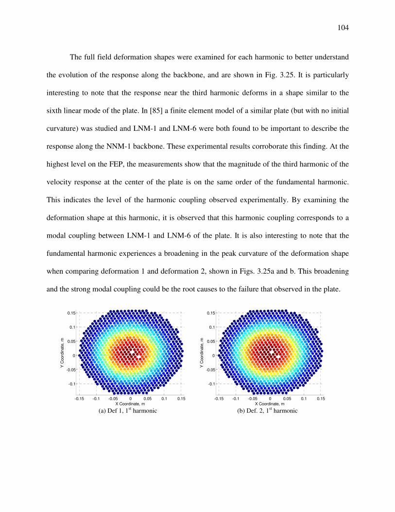
104

The full field deformation shapes were examined for each harmonic to better understand

the evolution of the response along the backbone, and are shown in Fig. 3.25. It is particularly

interesting to note that the response near the third harmonic deforms in a shape similar to the

sixth linear mode of the plate. In [85] a finite element model of a similar plate (but with no initial

curvature) was studied and LNM-1 and LNM-6 were both found to be important to describe the

response along the NNM-1 backbone. These experimental results corroborate this finding. At the

highest level on the FEP, the measurements show that the magnitude of the third harmonic of the

velocity response at the center of the plate is on the same order of the fundamental harmonic.

This indicates the level of the harmonic coupling observed experimentally. By examining the

deformation shape at this harmonic, it is observed that this harmonic coupling corresponds to a

modal coupling between LNM-1 and LNM-6 of the plate. It is also interesting to note that the

fundamental harmonic experiences a broadening in the peak curvature of the deformation shape

when comparing deformation 1 and deformation 2, shown in Figs. 3.25a and b. This broadening

and the strong modal coupling could be the root causes to the failure that observed in the plate.

-0.15 -0.1 -0.05 0 0.05 0.1 0.15

-0.1

-0.05

0

0.05

0.1

0.15

X Coordinate, m

Y C

oord

inate

, m

(a) Def 1, 1st harmonic

-0.15 -0.1 -0.05 0 0.05 0.1 0.15

-0.1

-0.05

0

0.05

0.1

0.15

X Coordinate, m

Y C

oord

inate

, m

(b) Def. 2, 1st harmonic

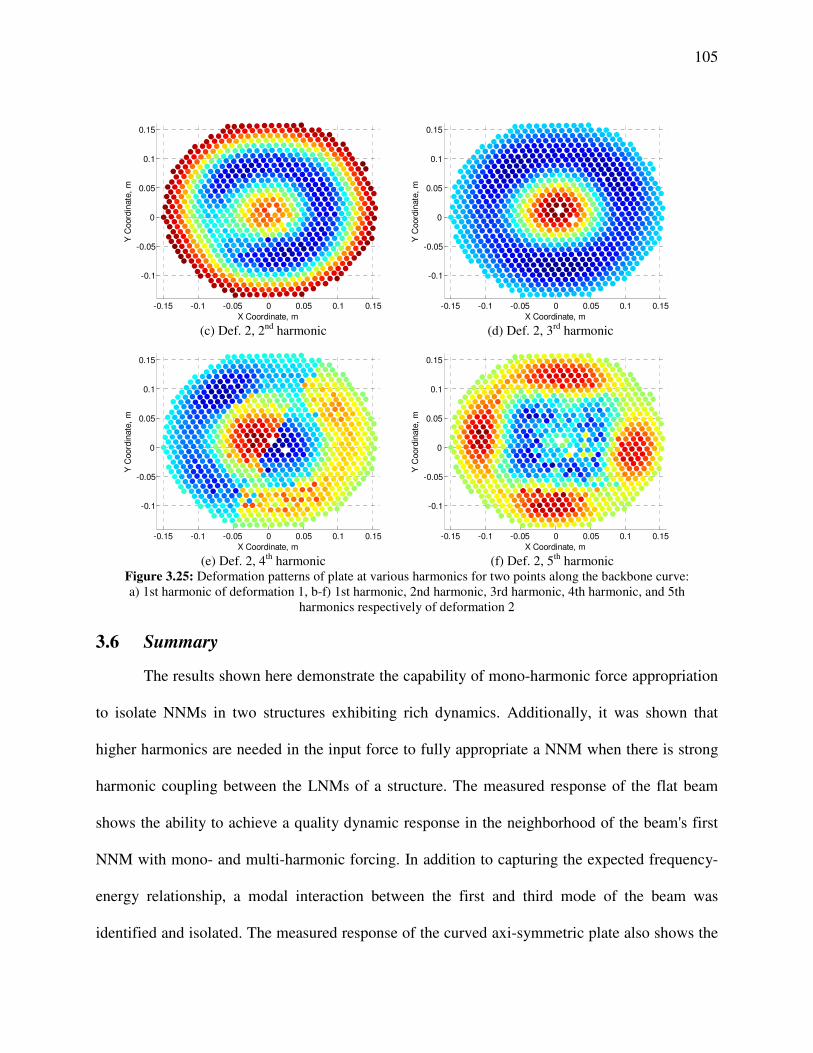
105

-0.15 -0.1 -0.05 0 0.05 0.1 0.15

-0.1

-0.05

0

0.05

0.1

0.15

X Coordinate, m

Y C

oord

inate

, m

(c) Def. 2, 2nd

harmonic

-0.15 -0.1 -0.05 0 0.05 0.1 0.15

-0.1

-0.05

0

0.05

0.1

0.15

X Coordinate, m

Y C

oord

inate

, m

(d) Def. 2, 3rd

harmonic

-0.15 -0.1 -0.05 0 0.05 0.1 0.15

-0.1

-0.05

0

0.05

0.1

0.15

X Coordinate, m

Y C

oord

inate

, m

(e) Def. 2, 4th

harmonic

-0.15 -0.1 -0.05 0 0.05 0.1 0.15

-0.1

-0.05

0

0.05

0.1

0.15

X Coordinate, m

Y C

oord

inate

, m

(f) Def. 2, 5th

harmonic

Figure 3.25: Deformation patterns of plate at various harmonics for two points along the backbone curve:

a) 1st harmonic of deformation 1, b-f) 1st harmonic, 2nd harmonic, 3rd harmonic, 4th harmonic, and 5th

harmonics respectively of deformation 2

3.6 Summary

The results shown here demonstrate the capability of mono-harmonic force appropriation

to isolate NNMs in two structures exhibiting rich dynamics. Additionally, it was shown that

higher harmonics are needed in the input force to fully appropriate a NNM when there is strong

harmonic coupling between the LNMs of a structure. The measured response of the flat beam

shows the ability to achieve a quality dynamic response in the neighborhood of the beam's first

NNM with mono- and multi-harmonic forcing. In addition to capturing the expected frequency-

energy relationship, a modal interaction between the first and third mode of the beam was

identified and isolated. The measured response of the curved axi-symmetric plate also shows the

106

ability to achieve a dynamic response in the neighborhood of the first NNM of a more complex

structure. The quality of the appropriated response for the plate was not on the same level of the

beam when looking at the phase of the input and response possibly demonstrating a limitation of

a mono-harmonic force to appropriate the response in the neighborhood of the expected NNM.

For both structures investigated, full-field deformation measurements were key to the

identification of nonlinear coupling between the LNMs of the structure. These measurements are

particularly beneficial when examining the more complex curved axi-symmetric plate, since the

ability of current modeling techniques limits the full examination of the structures nonlinear

properties. With the identification of the nonlinear coupling of the LNMs, experimental

nonlinear modal models can be created and tuned to better match the nonlinear dynamics. This

idea emphasizes an important area this work can be expanded upon where nonlinear modal

analysis techniques can be used to examine nonlinear coupling between LNMs tying together

linear and nonlinear experimental modal analysis.

107

4 Model Updating and Validation using Experimentally Measured Linear

and Nonlinear Normal Modes

4.1 Introduction

When the comparison between model and experiment reveals that the model is

inaccurate, it is important to determine which model parameters or features in the model should

be updated to improve the correlation. Typically, each of these parameters is slightly perturbed to

see whether they cause important changes in the validation metrics used (e.g. linear natural

frequencies and mode shapes). While brute force approaches based on optimization are used in

some applications, in this work the focus is on a physics based approach where the only

parameters updated are those that are justifiably uncertain.

Since elastic geometric nonlinear deformations are examined here, nominal dimensions

and material properties are used to build an initial model with the focus being the

characterization of the static equilibrium position. The error between the calculated and

measured natural frequencies are then used to update material properties and boundary

conditions providing models that better represent the structure's linear dynamics using well

established techniques [4]. Additionally, the structures' NNMs are used as a validation metric

after changes are made to the material properties and boundary conditions of the initial model

based on its linear modal parameters. Since NNMs are not directly used in the model updating

procedure, the updated models may or may not improve the correlation of the NNMs (e.g. the

extension of the linear modes to higher energy). Hence, the results show that it is critical to

simultaneously consider both the linear and the nonlinear behavior of the model in the model

updating process.

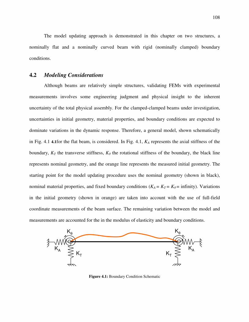
108

The model updating approach is demonstrated in this chapter on two structures, a

nominally flat and a nominally curved beam with rigid (nominally clamped) boundary

conditions.

4.2 Modeling Considerations

Although beams are relatively simple structures, validating FEMs with experimental

measurements involves some engineering judgment and physical insight to the inherent

uncertainty of the total physical assembly. For the clamped-clamped beams under investigation,

uncertainties in initial geometry, material properties, and boundary conditions are expected to

dominate variations in the dynamic response. Therefore, a general model, shown schematically

in Fig. 4.1 4.1for the flat beam, is considered. In Fig. 4.1, KA represents the axial stiffness of the

boundary, KT the transverse stiffness, Kθ the rotational stiffness of the boundary, the black line

represents nominal geometry, and the orange line represents the measured initial geometry. The

starting point for the model updating procedure uses the nominal geometry (shown in black),

nominal material properties, and fixed boundary conditions (KA = KT = Kθ = infinity). Variations

in the initial geometry (shown in orange) are taken into account with the use of full-field

coordinate measurements of the beam surface. The remaining variation between the model and

measurements are accounted for the in the modulus of elasticity and boundary conditions.

KT KT

KAKA

Kθ

Kθ

Figure 4.1: Boundary Condition Schematic

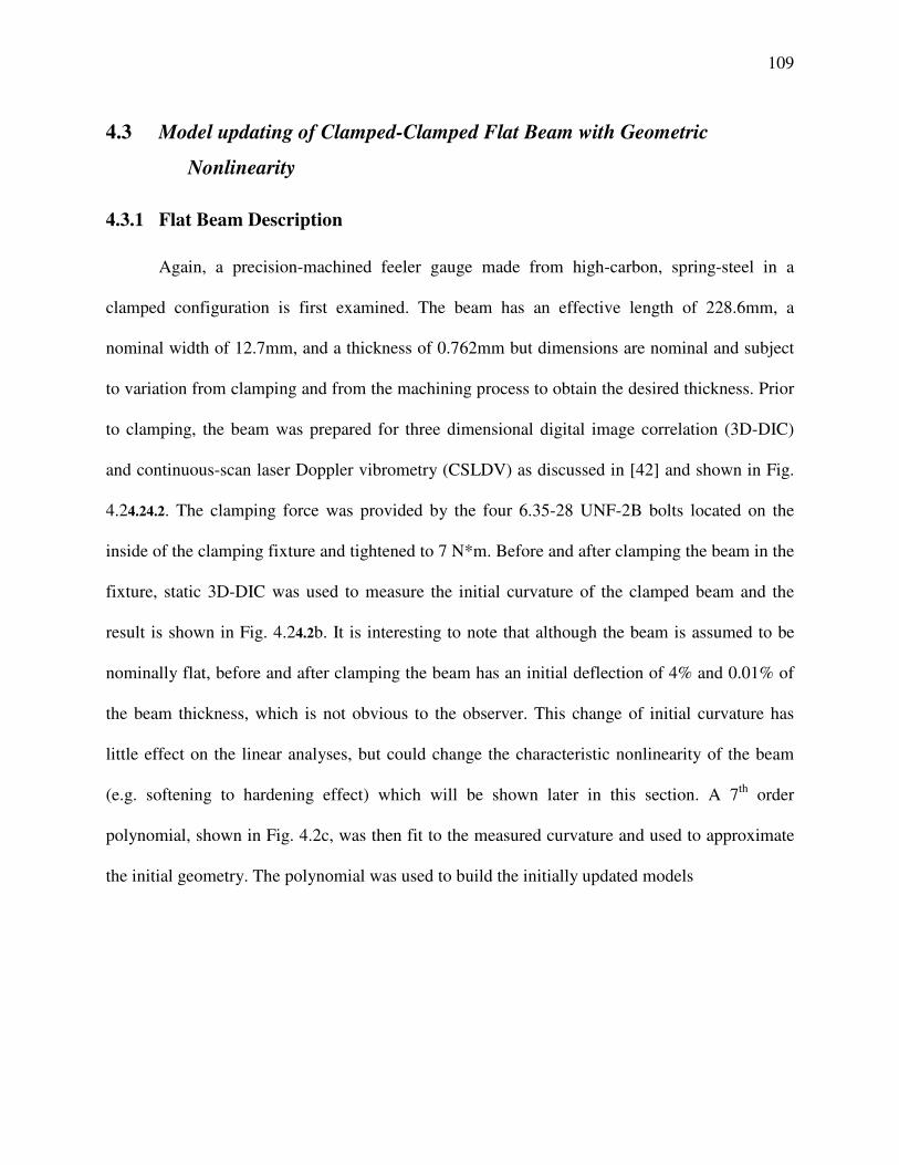
109

4.3 Model updating of Clamped-Clamped Flat Beam with Geometric

Nonlinearity

4.3.1 Flat Beam Description

Again, a precision-machined feeler gauge made from high-carbon, spring-steel in a

clamped configuration is first examined. The beam has an effective length of 228.6mm, a

nominal width of 12.7mm, and a thickness of 0.762mm but dimensions are nominal and subject

to variation from clamping and from the machining process to obtain the desired thickness. Prior

to clamping, the beam was prepared for three dimensional digital image correlation (3D-DIC)

and continuous-scan laser Doppler vibrometry (CSLDV) as discussed in [42] and shown in Fig.

4.24.24.2. The clamping force was provided by the four 6.35-28 UNF-2B bolts located on the

inside of the clamping fixture and tightened to 7 N*m. Before and after clamping the beam in the

fixture, static 3D-DIC was used to measure the initial curvature of the clamped beam and the

result is shown in Fig. 4.24.2b. It is interesting to note that although the beam is assumed to be

nominally flat, before and after clamping the beam has an initial deflection of 4% and 0.01% of

the beam thickness, which is not obvious to the observer. This change of initial curvature has

little effect on the linear analyses, but could change the characteristic nonlinearity of the beam

(e.g. softening to hardening effect) which will be shown later in this section. A 7th

order

polynomial, shown in Fig. 4.2c, was then fit to the measured curvature and used to approximate

the initial geometry. The polynomial was used to build the initially updated models

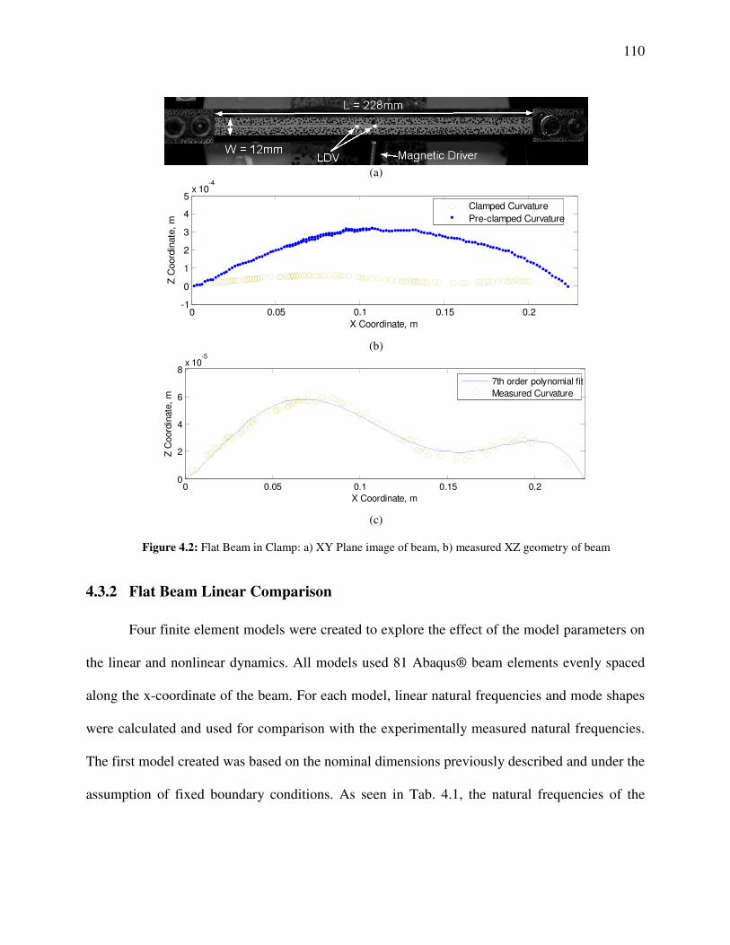
110

(a)

0 0.05 0.1 0.15 0.2-1

0

1

2

3

4

5x 10

-4

X Coordinate, m

Z C

oord

inate

, m

Clamped Curvature

Pre-clamped Curvature

(b)

0 0.05 0.1 0.15 0.20

2

4

6

8x 10

-5

X Coordinate, m

Z C

oord

inate

, m

7th order polynomial fit

Measured Curvature

(c)

Figure 4.2: Flat Beam in Clamp: a) XY Plane image of beam, b) measured XZ geometry of beam

4.3.2 Flat Beam Linear Comparison

Four finite element models were created to explore the effect of the model parameters on

the linear and nonlinear dynamics. All models used 81 Abaqus® beam elements evenly spaced

along the x-coordinate of the beam. For each model, linear natural frequencies and mode shapes

were calculated and used for comparison with the experimentally measured natural frequencies.

The first model created was based on the nominal dimensions previously described and under the

assumption of fixed boundary conditions. As seen in Tab. 4.1, the natural frequencies of the

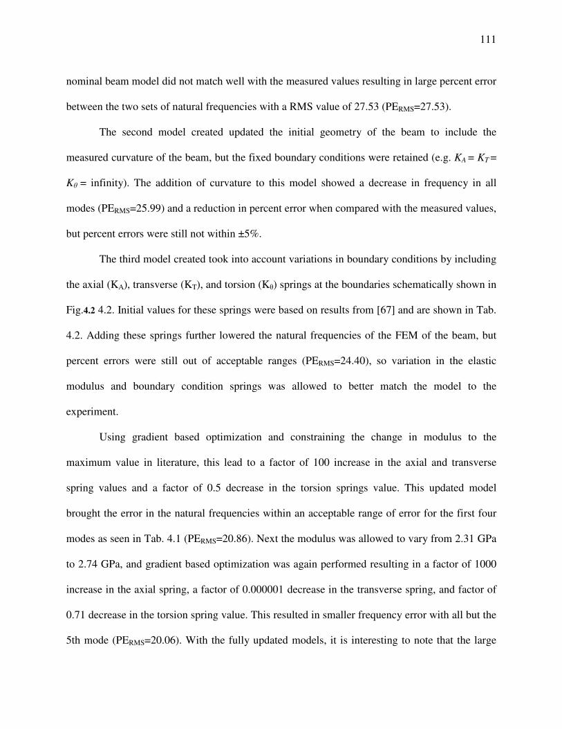
111

nominal beam model did not match well with the measured values resulting in large percent error

between the two sets of natural frequencies with a RMS value of 27.53 (PERMS=27.53).

The second model created updated the initial geometry of the beam to include the

measured curvature of the beam, but the fixed boundary conditions were retained (e.g. KA = KT =

Kθ = infinity). The addition of curvature to this model showed a decrease in frequency in all

modes (PERMS=25.99) and a reduction in percent error when compared with the measured values,

but percent errors were still not within ±5%.

The third model created took into account variations in boundary conditions by including

the axial (KA), transverse (KT), and torsion (Kθ) springs at the boundaries schematically shown in

Fig.4.2 4.2. Initial values for these springs were based on results from [67] and are shown in Tab.

4.2. Adding these springs further lowered the natural frequencies of the FEM of the beam, but

percent errors were still out of acceptable ranges (PERMS=24.40), so variation in the elastic

modulus and boundary condition springs was allowed to better match the model to the

experiment.

Using gradient based optimization and constraining the change in modulus to the

maximum value in literature, this lead to a factor of 100 increase in the axial and transverse

spring values and a factor of 0.5 decrease in the torsion springs value. This updated model

brought the error in the natural frequencies within an acceptable range of error for the first four

modes as seen in Tab. 4.1 (PERMS=20.86). Next the modulus was allowed to vary from 2.31 GPa

to 2.74 GPa, and gradient based optimization was again performed resulting in a factor of 1000

increase in the axial spring, a factor of 0.000001 decrease in the transverse spring, and factor of

0.71 decrease in the torsion spring value. This resulted in smaller frequency error with all but the

5th mode (PERMS=20.06). With the fully updated models, it is interesting to note that the large

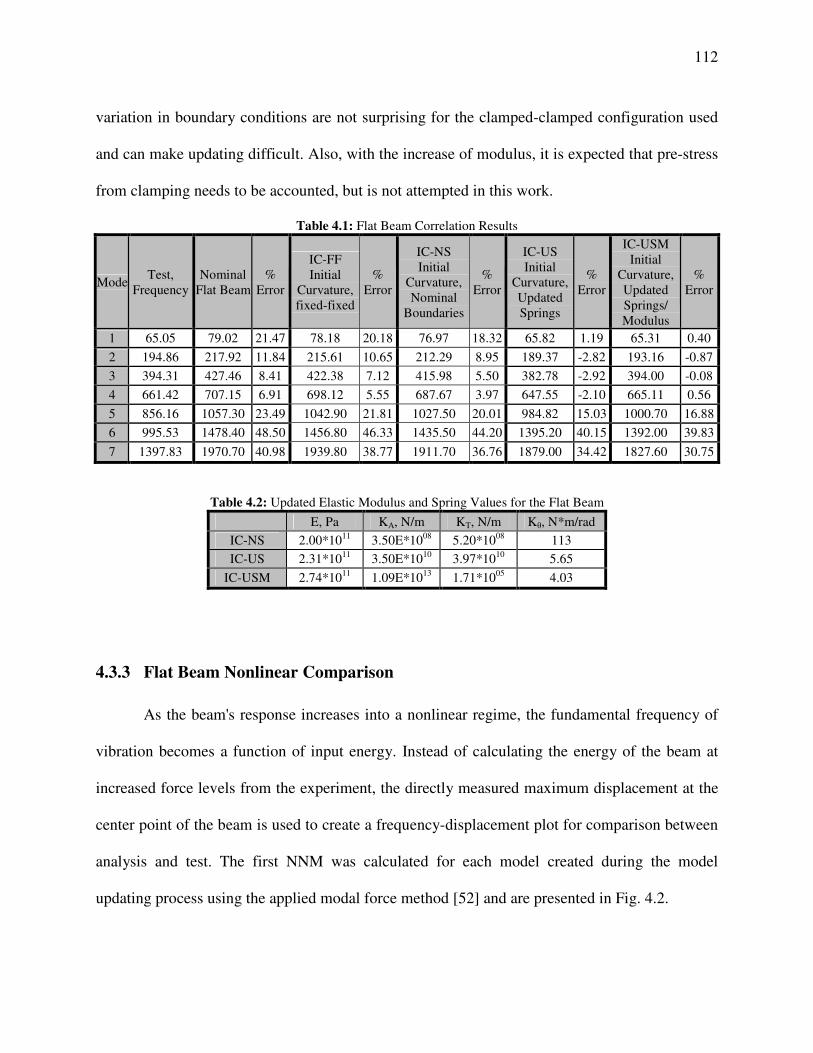
112

variation in boundary conditions are not surprising for the clamped-clamped configuration used

and can make updating difficult. Also, with the increase of modulus, it is expected that pre-stress

from clamping needs to be accounted, but is not attempted in this work.

Table 4.1: Flat Beam Correlation Results

ModeTest,

Frequency

Nominal

Flat Beam

%

Error

IC-FF

Initial

Curvature,

fixed-fixed

%

Error

IC-NS

Initial

Curvature,

Nominal

Boundaries

%

Error

IC-US

Initial

Curvature,

Updated

Springs

%

Error

IC-USM

Initial

Curvature,

Updated

Springs/

Modulus

%

Error

1 65.05 79.02 21.47 78.18 20.18 76.97 18.32 65.82 1.19 65.31 0.40

2 194.86 217.92 11.84 215.61 10.65 212.29 8.95 189.37 -2.82 193.16 -0.87

3 394.31 427.46 8.41 422.38 7.12 415.98 5.50 382.78 -2.92 394.00 -0.08

4 661.42 707.15 6.91 698.12 5.55 687.67 3.97 647.55 -2.10 665.11 0.56

5 856.16 1057.30 23.49 1042.90 21.81 1027.50 20.01 984.82 15.03 1000.70 16.88

6 995.53 1478.40 48.50 1456.80 46.33 1435.50 44.20 1395.20 40.15 1392.00 39.83

7 1397.83 1970.70 40.98 1939.80 38.77 1911.70 36.76 1879.00 34.42 1827.60 30.75

Table 4.2: Updated Elastic Modulus and Spring Values for the Flat Beam

E, Pa KA, N/m KT, N/m Kθ, N*m/rad

IC-NS 2.00*1011

3.50E*1008

5.20*1008

113

IC-US 2.31*1011

3.50E*1010

3.97*1010

5.65

IC-USM 2.74*1011

1.09E*1013

1.71*1005

4.03

4.3.3 Flat Beam Nonlinear Comparison

As the beam's response increases into a nonlinear regime, the fundamental frequency of

vibration becomes a function of input energy. Instead of calculating the energy of the beam at

increased force levels from the experiment, the directly measured maximum displacement at the

center point of the beam is used to create a frequency-displacement plot for comparison between

analysis and test. The first NNM was calculated for each model created during the model

updating process using the applied modal force method [52] and are presented in Fig. 4.2.

113

Fig. 4.2a shows the frequency-displacement plots for each step of the model updating,

and emphasizes that as the linear frequency converges to the desired value, the nonlinearity

experiences a drastic change in the frequency-energy relationship. By scaling the frequency of

the representative FEP to the model's linear natural frequency, this relationship is further

emphasized as seen in Fig. 4.2b. Starting with the flat fixed-fixed beam, shown in blue, the

nonlinear frequency-energy relation changes with each successive change in the model

parameters. The greatest change in the nonlinearity is observed when the initial curvature is

added to the model, shown in green. This occurs because a curved beam is less stiff axially, so as

bending and axial deformations couple, the stiffening effect on the bending modes is not as great

as with a flat beam. When compared with the flat fixed-fixed beam, the updated geometry

changed the first linear natural frequency 1.1% while the frequency-displacement relationship for

NNM 1 was reduced by approximately 50% for the input range investigated, showing the

sensitivity of the nonlinearity to initial geometry. With the addition of boundary condition

springs, the linear model showed a decrease of 1.5% of the first natural frequency, where NNM 1

showed an increase in the frequency-displacement relationship of 5%. This shows that the

relationship between the change in linear natural frequency and the nonlinear frequency-

displacement relationship is not linear in nature, as expected. The remaining two models showed

a larger change in the first linear natural frequency than in the nonlinear portion of the

representative FEP.

Based on the results of the comparison in Fig. 4.2 and Tab. 4.1 it appears that either of

the models denoted IC-US or IC-SM should accurately describe the dynamics of the beam when

dominated by the first mode. Improved accuracy in the nonlinear region of the model could be

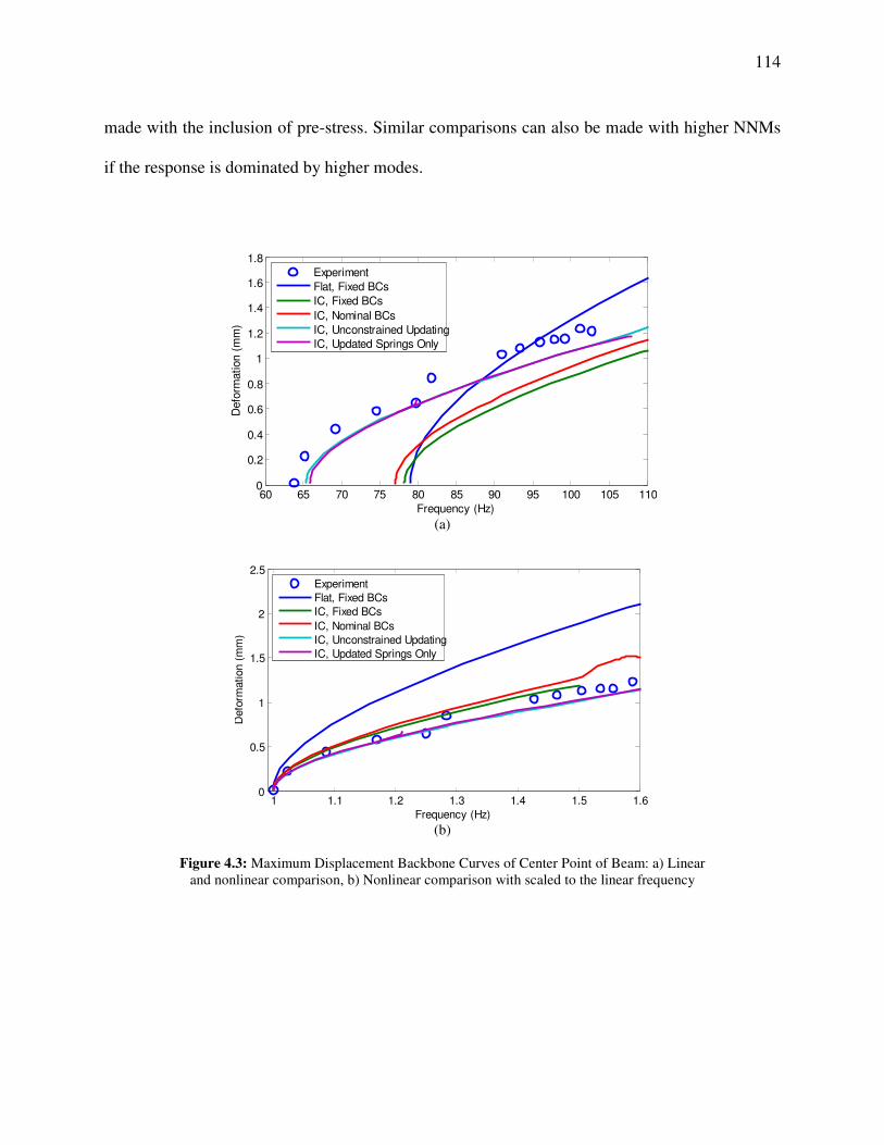
114

made with the inclusion of pre-stress. Similar comparisons can also be made with higher NNMs

if the response is dominated by higher modes.

60 65 70 75 80 85 90 95 100 105 1100

0.2

0.4

0.6

0.8

1

1.2

1.4

1.6

1.8

Frequency (Hz)

Defo

rmation (

mm

)

Experiment

Flat, Fixed BCs

IC, Fixed BCs

IC, Nominal BCs

IC, Unconstrained Updating

IC, Updated Springs Only

(a)

1 1.1 1.2 1.3 1.4 1.5 1.60

0.5

1

1.5

2

2.5

Frequency (Hz)

Defo

rmation (

mm

)

Experiment

Flat, Fixed BCs

IC, Fixed BCs

IC, Nominal BCs

IC, Unconstrained Updating

IC, Updated Springs Only

(b)

Figure 4.3: Maximum Displacement Backbone Curves of Center Point of Beam: a) Linear

and nonlinear comparison, b) Nonlinear comparison with scaled to the linear frequency

115

4.4 Model updating of Clamped-Clamped Curved Beam with Geometric

Nonlinearity

4.4.1 Curved Beam Description

The second structure investigate is a cold rolled curved beam made from high-carbon,

spring-steel in a clamped configuration. The beam has an effective length of 304.85mm, a

nominal width of 12.7mm, and a thickness of 0.508mm. The cold rolling was done to induce an

initial curvature of 3048mm, but as with the flat beam, all presented dimensions are nominal and

subject to variation. The clamping force was provided by the two 6.35-28 UNF-2B bolts located

on the inside of the clamping fixture, which is the same fixture used in [39].

Before and after clamping the beam in the fixture, static 3D-DIC was again used to

measure the initial curvature of the clamped beam as shown in Fig. 4.4b. It is observed here that

the clamping induces an asymmetric preload to the final configuration of the beam, which is not

accounted for in the model. Similar to the flat beam, an 8th

order polynomial was then fit to the

measured curvature and used to approximate the initial geometry of the beam as shown in Fig.

4.4c. As with the flat beam, single-input single-output modal hammer tests were performed

throughout testing on the curved beam to identify natural frequencies and damping ratios.

Results from these hammer tests showed a 7% variation in the first natural frequency of the final

clamped beam, which can be expected due to the variation in the experimental setup.

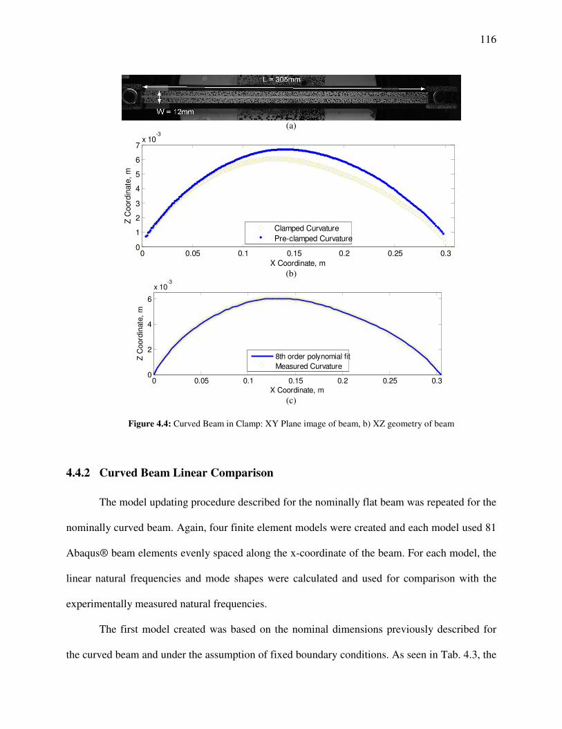
116

(a)

0 0.05 0.1 0.15 0.2 0.25 0.30

1

2

3

4

5

6

7x 10

-3

X Coordinate, m

Z C

oord

inate

, m

Clamped Curvature

Pre-clamped Curvature

(b)

0 0.05 0.1 0.15 0.2 0.25 0.30

2

4

6

x 10-3

X Coordinate, m

Z C

oord

inate

, m

8th order polynomial fit

Measured Curvature

(c)

Figure 4.4: Curved Beam in Clamp: XY Plane image of beam, b) XZ geometry of beam

4.4.2 Curved Beam Linear Comparison

The model updating procedure described for the nominally flat beam was repeated for the

nominally curved beam. Again, four finite element models were created and each model used 81

Abaqus® beam elements evenly spaced along the x-coordinate of the beam. For each model, the

linear natural frequencies and mode shapes were calculated and used for comparison with the

experimentally measured natural frequencies.

The first model created was based on the nominal dimensions previously described for

the curved beam and under the assumption of fixed boundary conditions. As seen in Tab. 4.3, the

117

natural frequencies of the nominal beam model again did not match well with the measured

values as the percent frequency error between the models had an RMS value of 16.98

(PERMS=16.98).

The second model created updated the initial geometry of the beam to include the

measured curvature of the beam, but the fixed boundary conditions were retained (e.g. KA = KT =

Kθ = infinity). The addition of curvature to this model showed an increase in frequency in all

modes and a reduction in frequency errors (PERMS=4.41) when compared with the measured

values, with modes 4 and 5 outside the desired ±5%.

Since a similar clamp was used, the third model created used the same nominal values for

the boundary condition springs that were used for the flat beam as shown in Tab. 4.4. The

addition of these springs had varying effects to the natural frequencies of the beam

(PERMS=4.03), but the frequency errors for modes 4 and 5 were still larger than desired.

The elastic modulus and boundary condition springs were varied using gradient based

optimization while also constraining the change in modulus to the maximum value in literature.

This lead to a factor of 107 increase in the axial spring stiffness, a factor of 100 increase in

transverse spring, and a factor of 6000 increase in the torsion springs value. This updated model

reduced the error in modes 4 and 5, but overall the errors in the natural frequencies (PERMS=7.02)

are larger than for the model with nominal boundary springs and the large error in the first

natural frequency is certainly a concern.

Finally, the modulus was allowed to vary from 2.31 GPa to 2.76 GPa, and gradient based

optimization was again performed resulting in a factor of 105 increase in the axial spring and no

change in the transverse and torsion spring values. This updated model brought all natural

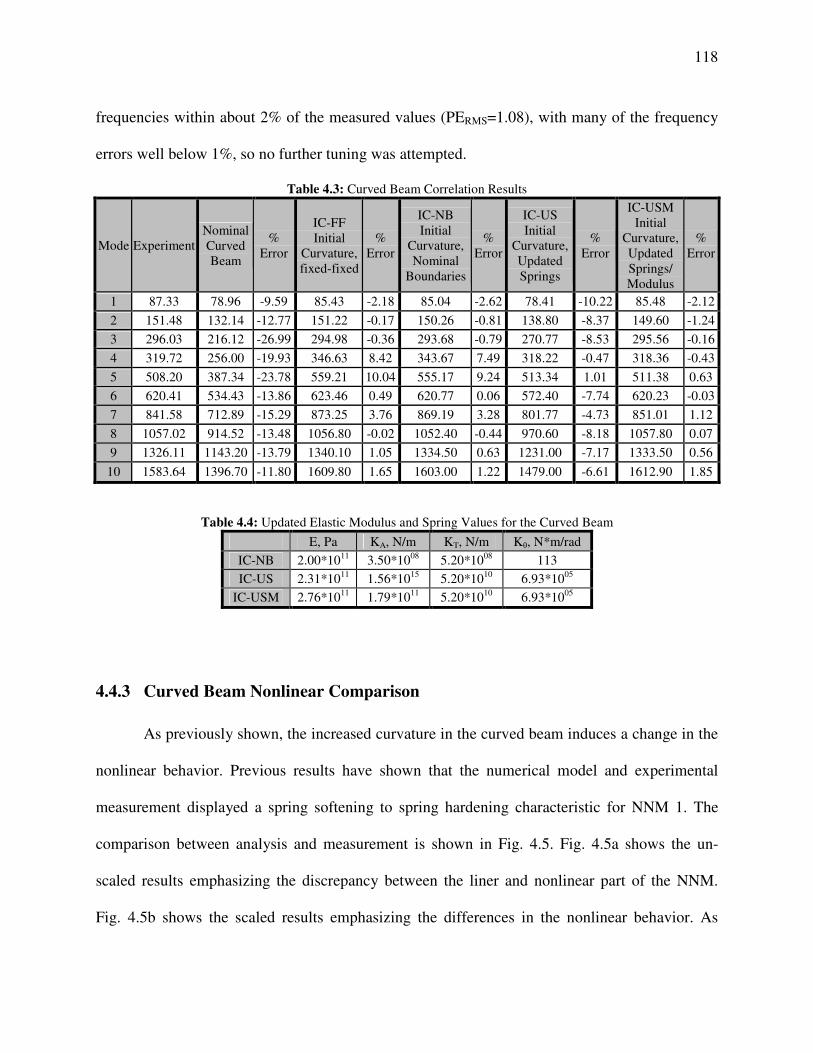
118

frequencies within about 2% of the measured values (PERMS=1.08), with many of the frequency

errors well below 1%, so no further tuning was attempted.

Table 4.3: Curved Beam Correlation Results

Mode Experiment

Nominal

Curved

Beam

%

Error

IC-FF

Initial

Curvature,

fixed-fixed

%

Error

IC-NB

Initial

Curvature,

Nominal

Boundaries

%

Error

IC-US

Initial

Curvature,

Updated

Springs

%

Error

IC-USM

Initial

Curvature,

Updated

Springs/

Modulus

%

Error

1 87.33 78.96 -9.59 85.43 -2.18 85.04 -2.62 78.41 -10.22 85.48 -2.12

2 151.48 132.14 -12.77 151.22 -0.17 150.26 -0.81 138.80 -8.37 149.60 -1.24

3 296.03 216.12 -26.99 294.98 -0.36 293.68 -0.79 270.77 -8.53 295.56 -0.16

4 319.72 256.00 -19.93 346.63 8.42 343.67 7.49 318.22 -0.47 318.36 -0.43

5 508.20 387.34 -23.78 559.21 10.04 555.17 9.24 513.34 1.01 511.38 0.63

6 620.41 534.43 -13.86 623.46 0.49 620.77 0.06 572.40 -7.74 620.23 -0.03

7 841.58 712.89 -15.29 873.25 3.76 869.19 3.28 801.77 -4.73 851.01 1.12

8 1057.02 914.52 -13.48 1056.80 -0.02 1052.40 -0.44 970.60 -8.18 1057.80 0.07

9 1326.11 1143.20 -13.79 1340.10 1.05 1334.50 0.63 1231.00 -7.17 1333.50 0.56

10 1583.64 1396.70 -11.80 1609.80 1.65 1603.00 1.22 1479.00 -6.61 1612.90 1.85

Table 4.4: Updated Elastic Modulus and Spring Values for the Curved Beam

E, Pa KA, N/m KT, N/m Kθ, N*m/rad

IC-NB 2.00*1011

3.50*1008

5.20*1008

113

IC-US 2.31*1011

1.56*1015

5.20*1010

6.93*1005

IC-USM 2.76*1011

1.79*1011

5.20*1010

6.93*1005

4.4.3 Curved Beam Nonlinear Comparison

As previously shown, the increased curvature in the curved beam induces a change in the

nonlinear behavior. Previous results have shown that the numerical model and experimental

measurement displayed a spring softening to spring hardening characteristic for NNM 1. The

comparison between analysis and measurement is shown in Fig. 4.5. Fig. 4.5a shows the un-

scaled results emphasizing the discrepancy between the liner and nonlinear part of the NNM.

Fig. 4.5b shows the scaled results emphasizing the differences in the nonlinear behavior. As

119

shown in Fig. 4.5b, the nominally curved model, shown with a blue line, and the experiment,

shown with blue circles, show a large difference in the "turning point", or change from spring

softening to spring hardening, of the characteristic FEP. When the initial curvature of the beam is

changed to match the measured shape of the beam, the result shown with a green line reveals that

the characteristic of the nonlinearity changes to initially spring hardening and then spring

softening; this is the opposite of what is observed experimentally. So, even though this change to

the model improves the correspondence of the linear natural frequencies, this comparison reveals

that the model now represents the nonlinear behavior less accurately.

The models IC-NB and IC-US with nominal and updated values for the boundary

condition springs also predict initial hardening and then softening, further underscoring the fact

that updating the model based on its linear behavior alone is not sufficient to bring the nonlinear

behavior into agreement. It is also interesting to note that while the large changes (107 change in

axial spring, 102 change in transverse spring, and the 10

3 change in torsion spring) change the

location of the turning point in the FEP, the hardening to softening characteristic is maintained;

apparently this characteristic is a function of the geometry alone or of some other parameter that

was not considered. Although the linear portion of the fully updated model matches experiment

well, it does not do any better at capturing the nonlinearity. So, further updating will be needed

to bring this model into correspondence with measurements. Considering Fig. 4.4, it could be

posed that pre-stress in the beam due to clamping into the fixture may be important, so it will be

allowed to vary in future models.

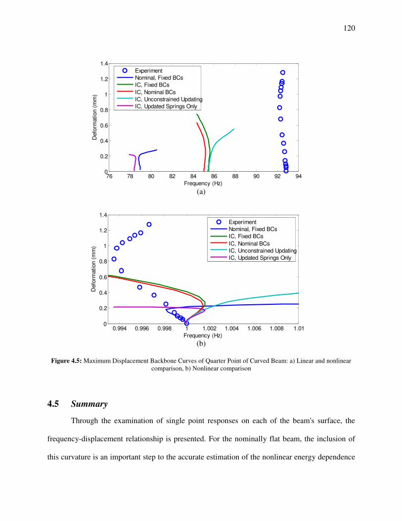
120

76 78 80 82 84 86 88 90 92 940

0.2

0.4

0.6

0.8

1

1.2

1.4

Frequency (Hz)

Defo

rmation (

mm

)

Experiment

Nominal, Fixed BCs

IC, Fixed BCs

IC, Nominal BCs

IC, Unconstrained Updating

IC, Updated Springs Only

(a)

0.994 0.996 0.998 1 1.002 1.004 1.006 1.008 1.010

0.2

0.4

0.6

0.8

1

1.2

1.4

Frequency (Hz)

Defo

rmation (

mm

)

Experiment

Nominal, Fixed BCs

IC, Fixed BCs

IC, Nominal BCs

IC, Unconstrained Updating

IC, Updated Springs Only

(b)

Figure 4.5: Maximum Displacement Backbone Curves of Quarter Point of Curved Beam: a) Linear and nonlinear

comparison, b) Nonlinear comparison

4.5 Summary

Through the examination of single point responses on each of the beam's surface, the

frequency-displacement relationship is presented. For the nominally flat beam, the inclusion of

this curvature is an important step to the accurate estimation of the nonlinear energy dependence

121

of the fundamental frequency of vibration. Additionally, through the change of boundary

conditions, this energy dependence can be tuned to match experimental measurements. Here, it is

important to include axial and transverse springs due to the small initial curvature. If the beam

was flat, only axial springs would be needed for model updating and tuning of the nonlinearity,

but for the presented results, the transverse springs were as significant as the axial springs. For

the nominally curved beam, changing the curvature and boundary conditions has been shown to

change the fundamental characteristic of the nonlinearity inherent to the structure. Therefore,

more care must be taken in the model updating procedure to ensure that the true nonlinearity is

accounted.

Future work will seek to add effects from asymmetries and pre-stress induced from

clamping. With the use of NNM force appropriation and full-field measurements, as described in

[45], an examination of the effect of asymmetries to the dynamic response is possible. With the

examination of the change in mode shapes at higher response levels, more insight can be gained

for the improved correlation of the nonlinearity, which would be especially information for

structures with complex changes in nonlinearity (e.g. the curved beam). Also, work will seek to

use NNM backbones as a quantitative metric for nonlinear model updating using a global metric

instead of through the uses of full-field experimental and numerical data examining only single

location responses. The addition of full-field deformations shapes gives additional clues about

how we might need to update the model to improve validation of the NNMs.

122

5 Summary

This dissertation has contributed to the state of the art in several areas. First, two

advanced full field measurement methodologies were compared and found to be useful when

characterizing nonlinear deformations of thin structures. The full field measurements that they

provide were found to give unique insights into how the linear modes couple, information which

could be helpful when creating or updating reduced order models. Second, new metrics were

developed that simplify the process of isolating an NNM in a measurement using stepped-sine

testing. The metrics were validated in simulation and experiments were presented in which an

internal resonance was isolated for the first time (although with some inaccuracy due to the

experimental setup). Finally, these methods were applied to nonlinear model updating of several

geometrically nonlinear structures producing encouraging results. These contributions are

discussed in more detail below.

5.1 Continuous-scan Laser Doppler Vibrometry and Three Dimensional-

Digital Image Correlation

In Chapter 2 it was shown that Continuous-scan Laser Doppler Vibrometry (CSLDV) and

Three Dimensional-Digital Image Correlation (3D-DIC) can be used to obtain full-field

measurements of a structure vibrating in linear and nonlinear response regimes. This was

demonstrated on two structures: a clamped-clamped flat beam and a fully clamped flat plate. For

low amplitude, linear deformations, it was shown that CSLDV was able to reconstruct the

measured deformation shapes more accurately than 3D-DIC due to 3D-DIC's limited resolution

at low amplitudes. When using CSLDV, the spatial measurement information is not governed by

the number of points used to define the shape but by the number of Fourier coefficients that can

123

be identified to describe the time-varying shape. The number of harmonics is especially

important when a more complex 2-D measurement grid is used, as demonstrated with the flat

panel. Hence, the main disadvantage of CSLDV is that the harmonics describing the shapes are

measured rather than the shapes at individual points, and so there may be uncertainty as to

whether a feature in the measured deformation is really meaningful. For higher amplitude,

nonlinear deformations, 3D-DIC was shown to reconstruct more complex spatial deformations at

higher harmonics more accurately than CSLDV, further emphasizing the reliance of higher

harmonics for the correct reconstruction of the deformation shape.

Both techniques can provide dense measurements along surfaces, as long as each

technique can "see" the surface. To provide accurate measurements, both techniques require

surface preparation, unless the material used for the test piece fulfills specific requirements (e.g.

a random pattern for 3D-DIC and a sufficiently reflective pattern for CSLDV). For DIC, this

surface preparation is especially important when response levels are small, or in a structure's

linear range. For CSLDV, surface preparation becomes more important when the vibration

amplitude becomes small relative to speckle noise, and also as the laser standoff distance (or

field of view) increases.

Finally, this study has illustrated that when full-field velocities or displacements are

measured (i.e. as opposed to the usual case where the motion is only captured at a few points),

inconsistencies in the dynamic behavior of the structure under test can be identified and provide

insight to modeling and predicting dynamic behavior. Here, the CSLDV and DIC shapes

revealed asymmetry in the 2nd and 3rd bending mode shapes of the beam and a skew in mode 1

of the bending mode shape of the plate, which was probably due to (un-modeled) asymmetry in

the boundary conditions or initial geometry of the plate since it is thin. If a traditional test were

124

performed with only a few measurement points, one would not be likely to detect this, nor would

they have sufficient information to update the model to account for it.

5.2 Experimental Identification of Nonlinear Normal Modes

In Chapter 3, a method to determine the numerical and experimental single point force

needed to appropriate a nonlinear normal mode (NNM) was demonstrated on a clamped-clamped

flat beam and curved axi-symmetric perforated plate. It was shown that higher harmonics are

needed in the input force to fully appropriate a NNM when there is strong harmonic coupling

between the LNMs of a structure. For both structures, a strong harmonic coupling was observed,

5:1 coupling for the flat beam and a 3:1 coupling for the curved axi-symmetric plate. The

measured response of the flat beam shows the ability to achieve an appropriated NNM response

in the neighborhood of the beam's first NNM with mono- and multi-harmonic forcing. The

measured response of the curved axi-symmetric plate also shows the ability to achieve a dynamic

response in the neighborhood of the first NNM of a more complex structure.

For both structures investigated, full-field deformation measurements were key to the

identification of nonlinear coupling between the LNMs of the structure. These measurements are

particularly beneficial when examining the more complex curved axi-symmetric plate. With the

identification of the nonlinear coupling of the LNMs, experimental nonlinear modal models can

be created and tuned to better match the nonlinear dynamics. This idea emphasizes an important

area this work can be expanded upon where nonlinear modal analysis techniques can be used to

examine nonlinear coupling between LNMs tying together linear and nonlinear experimental

modal analysis.

125

5.3 Model Updating and Validation using Experimentally and Numerically

Determined Linear and Nonlinear Normal Modes

Through the examination of single point responses on each of the beam's surface, the

frequency-displacement relationship is presented. For the geometrically nonlinear beams

investigated, the inclusion of this curvature is an important step to the accurate estimation of the

nonlinear energy dependence of the fundamental frequency of vibration. Additionally, through

the change of boundary conditions, this energy dependence can be further tuned to match

experimental measurements. For the nominally flat beam, this resulted in a well tuned model;

however, this was not the case for the beam with an initial curvature. For the curved beam,

changing the curvature and boundary conditions change the fundamental characteristic of the

nonlinearity inherent to the structure so, more care must be taken in the model updating

procedure to determine which features in the model need to be updated. In this regard, it is

hoped that full field measurements will provide insights into what changes to the model are

needed.

126

6 Future Work

6.1 Characterization and Optimization of Experimental Setup for Continuous-

scan Laser Doppler Vibrometry and Three Dimensional-Digital Image

Correlation

Continuous-scan Laser Doppler Vibrometry (CSLDV) and Three Dimensional-Digital

Image Correlation (3D-DIC) was successfully used to measure the full-field linear and nonlinear

deformations of a structure; however, the use of each technique is currently more of an art than a

science. For CSLDV, parameters such as the laser standoff distance, scan frequency, and scan

pattern are selected based on the experimenter's experience and knowledge of the structural

response being measured. An experienced operator typically needs to perform trial and error

experiments when a structure exhibits unexpected responses. For 3D-DIC, parameters such as

the camera standoff distance, camera angle, calibration parameters, and application of speckle

pattern are based on the experimenter's experience and knowledge of the interaction between all

parameters in the measured of a deforming structure. Similar to CSLDV, a series of trial and

error experiments are needed to find an optimal setup. Both measurement methods would benefit

from a more formal definition of the optimum experimental parameters used.

6.2 Experimental Identification of Nonlinear Normal Modes

The presented methods developed to isolate the nonlinear normal modes (NNMs) of a

structure require much user interaction. Therefore, the identification of NNMs is dependent on

the experimenters knowledge of how the damped forced response manifests in nonlinear

regimes. Automation of the identification of NNMs is further complicated since structures

127

exhibit dynamics such as jumps, quasi- or fully chaotic responses requiring a continuous tuning

of the force distribution and harmonic content step size used in the isolation of an NNM to

remain on a forced response curve. The use of power balance methods along with real time tonal

analysis methods to determine the phase relationships between the force and response at all

harmonics dynamically would be one path to the development of automatic NNM identification

algorithms.

6.3 Update Models using Nonlinear Normal Modes

As shown, nonlinear normal modes (NNMs) provide a useful representation of a

structure's bifurcations, internal resonances, and a strong dependence on input energy through

the use of frequency energy plots (FEPs). Additionally, the time-series domain of the periodic

solutions for each harmonic provides a description of how higher harmonics appear in the

response throughout increasingly nonlinear response regimes. This response can be projected

onto the linear normal modes (LNMs) of the response providing a characterization of the

nonlinear coupling of the LNMs over desired ranges of the dynamic response.

6.4 Model Validation using Nonlinear Measured and Simulated Responses

Though NNMs provide an excellent tool to validate a model in nonlinear response

regimes, it is also beneficial to further validate the updated models when subjected to other types

of loading. Therefore, during previous testing, additional low and high amplitude response data

was measured when the structures of interest were subjected to a band limited random excitation.

This random response data can be used to validate the fully updated models through the

examination of the measured and simulated response power spectral densities (PSDs).

Schoneman et al. [106] recently used this type of model validation to validate nonlinear reduced

128

order models (NLROMs) of a flat beam. It was observed that the coupled dynamics between

mode 1, 3, and 5 was key to the accurate prediction of the response PSDs. Without the inclusion

of mode 1, the response PSD did not capture the nonlinear behavior of the flat beam investigated.

A similar use of the response PSDs will be implemented to provide a final validation step for the

fully updated models.

Acknowledgements

Support for this research was provided by the University of Wisconsin – Madison

Graduate School with funding from the Wisconsin Alumni Research Foundation and through the

Structural Sciences Center in the Air Force Research Laboratory's summer internship program.

129

Appendix – Publications of PhD work

Journal Papers

• Ehrhardt, D.A., Yang, S., Beberniss, T.J., and Allen, M.S., "Full Field Measurements of beams and

plates with Continuous-Scan Laser Doppler Vibrometry and 3D-Digital Image Correlation,"

Mechanical Systems and Signal Processing (Submitted)

• Ehrhardt, D.A., Allen, M.S., and Beberniss, T.J., "Measurement of Nonlinear Normal Modes using

Mono-Harmonic Force Appropriation and Full Field Measurements," Mechanical Systems and Signal

Processing Special Issue Dedicated to the Identification of Nonlinear Mechanical Systems (in

preparation)

• Ehrhardt, D.A. and Allen, M.S., "Model Updating of Geometrically Nonlinear Flat and Curved

Beam with Nonlinear Normal Modes," AIAA Journal (in preparation)

Conference Papers

• Ehrhardt, D.A., Yang, S., Beberniss, T.J., and Allen, M.S., " Linear and Nonlinear Response of a

Rectangular Plate Measured with Continuous-Scan Laser Doppler Vibrometry and 3D-Digital Image

Correlation," 33rd

International Modal Analysis Conference, February 2-5, 2015.

• Ehrhardt, D.A., Allen, M.S., " Measurement of Nonlinear Normal Modes using Mono-harmonic

Force Appropriation: Experimental Investigation," 33rd

International Modal Analysis Conference,

February 2-5, 2015.

• Ehrhardt, D.A., Kuether, R.J., and Allen, M.S., "Nonlinear Normal Modes in Finite Element Model

Validation of Geometrically Nonlinear Flat and Curved Beams," AIAA SciTech 2015, January 5-9,

2015.

• Ehrhardt, D.A., Yang, S., Beberniss, T.J., and Allen, M.S., "Mode Shape Comparison Using

Continuous-scan Laser Doppler Vibrometry and High Speed 3D Digital Image Correlation," 32nd

International Modal Analysis Conference, February 3-6, 2014.

130

• Ehrhardt, D.A., Harris, R.B., and Allen, M.S., "Numerical and Experimental Determination of

Nonlinear Normal Modes of a Circular Perforated Plate," 32nd

International Modal Analysis

Conference, February 3-6, 2014.

• Ehrhardt, D.A. and Beberniss, T.J., "Experimental Investigation of Dynamic out of Plane

Displacement Error in 3D Digital Image Correlation," AIAA Conference, April 8-11, 2013. DOI:

10.2514/6.2013-1779.

• Ehrhardt, D.A., Abanto-Bueno, J.A., Shukla, A., and Parks, C., "Non-contact Experimental Modal

Analysis of a Curved Beam using a Full-Field Optical Technique," AIAA, April 4-7, 2011. DOI:

10.2514/6.211-1945.

131

References

[1] ASME, "Guide for Verification and Validation in Computational Solid Mechanics," vol.

V V 10-2006, ed, 2006.

[2] R. J. Allemang, "Editorial: Verification and Validation," Sound and Vibration, January

2013.

[3] J. H. Ginsberg, Mechanical and Structural Vibrations, First ed. New York: John Wiley

and Sons, 2001.

[4] M. I. Friswell, and Mottershead, J.E., Finite Element Model Updating in Structural

Dynamics: Kluwer Academic Publishers, 1995.

[5] D. J. Ewins, Modal Analysis Theory, Practice, and Application, Second Edition ed.:

Research Studies Press Ltd., 2000.

[6] T. Abrahamsson, and Kammer, D., "Finite Element Model Calibration using Frequency

Responses and Damping Equalization," presented at the 32nd International Modal

Analysis Conference, Orlando, FL., 2013.

[7] R. J. Allemang, "The Modal Assurance Criterion (MAC): Twenty Years of Use and

Abuse," in XX International Modal Analysis Conference, Los Angeles, CA, 2002.

[8] R. R. Craig, and Kurdila, A.J., Fundamentals of Structural Dynamics, 2nd ed.: Wiley,

2006.

[9] A. B. Stanbridge and D. J. Ewins, "Modal Testing Using a Scanning Laser Doppler

Vibrometer," Mechanical Systems and Signal Processing, vol. 13, pp. 255-270, 1999.

[10] M. A. Sutton, Orteu, J.J., and Schreier, H., Image Correlation for Shape, Motion, and

Deformation Measurements: Basic Concepts, Theory, and Applications. New York, NY:

Springer, 2009.

[11] R. M. Rosenberg, "Normal Modes of Nonlinear Dual-Mode Systems," Journal of Applied

Mechanics, vol. 27, pp. 263-268, 1960.

[12] A. F. Vakakis, Manevitch, L.I., Mikhlin, Y.V., Pilipchuk, V.M., and Zeven, A.A.,

Normal Modes and Localization in Nonlinear Systems. New York: John Wiley & Sons,

1996.

[13] G. Kerschen, M. Peeters, J. C. Golinval, and A. F. Vakakis, "Nonlinear normal modes,

Part I: A useful framework for the structural dynamicist," Mechanical Systems and Signal

Processing, vol. 23, pp. 170-194, 2009.

[14] A. H. Nayfeh, Nonlinear Interactions: Analytical, Computational, and Experimental

Methods. New Your, NY, 2000.

[15] A. H. Nayfeh, Nonlinear Oscillations. New York: John Wiley and Sons, 1979.

[16] M. Peeters, G. Kerschen, and J. C. Golinval, "Modal testing of nonlinear vibrating

structures based on nonlinear normal modes: Experimental demonstration," Mechanical

Systems and Signal Processing, vol. 25, pp. 1227-1247, 2011.

[17] J. L. Zapico-Valle and M. García-Diéguez, "Dynamic modeling and identification of the

Uniovi structure," Int. J. Simul. Multidisci. Des. Optim., vol. 5, p. A06, 2014.

[18] G. Kerschen, K. Worden, A. F. Vakakis, and J.-C. Golinval, "Past, present and future of

nonlinear system identification in structural dynamics," Mechanical Systems and Signal

Processing, vol. 20, pp. 505-592, 2006.

132

[19] M. Kurt, "Identificatoin, Reduced Order Modeling, and Model Updating of Nonlinear

Mechanical Systems," PhD, Mechanical Engineering, University of Illinois at Urbana-

Champaign, Urbana, Illinois, 2014.

[20] J. P. Noel, Renson, L., Grappasonni, C., and Kerschen, G., "Identification of Nonlinear

Normal Modes of Engineering Structures under Broadband Forcing," Mechanical

Systems and Signal Processing.

[21] M. Peeters, G. Kerschen, and J. C. Golinval, "Dynamic testing of nonlinear vibrating

structures using nonlinear normal modes," Journal of Sound and Vibration, vol. 330, pp.

486-509, 2011.

[22] P. A. Atkins, Wright, J.R., and Worden, K., "An Extension of Force Appropriation to the

Identification of Nonlinear Multi Degree of Freedom Systems," Journal of Sound and

Vibration, vol. 237, pp. 23-43, 2000.

[23] N. M. Wereley, "Analysis and Control of Linear Periodically Time Varying Systems,"

Ph.D. Ph.D., Aeronautics and Astronautics, Massachusetts Institute of Technology,

Cambridge, 1991.

[24] A. B. Stanbridge, D. J. Ewins, and A. Z. Khan, "Modal testing using impact excitation

and a scanning LDV," Shock & Vibration, vol. 7, p. 91, 2000.

[25] M. Martarelli, "Exploiting the Laser Scanning Facility for Vibration Measurements,"

Ph.D. Ph.D. , Technology & Medice, Imperial College, London, 2001.

[26] A. B. Stanbridge, M. Martarelli, and D. J. Ewins, "Measuring area vibration mode shapes

with a continuous-scan LDV," Measurement, vol. 35, pp. 181-189, 2004.

[27] C. W. Schwingshackl, A. B. Stanbridge, C. Zang, and D. J. Ewins, "Full-Field Vibration

Measurement of Cylindrical Structures using a Continuous Scanning LDV Technique,"

presented at the 25th International Modal Analysis Confernce (IMAC XXV), Orlando,

Florida, 2007.

[28] M. S. Allen, "Frequency-Domain Identification of Linear Time-Periodic Systems using

LTI Techniques," Journal of Computational and Nonlinear Dynamics vol. 4, 24 Aug.

2009.

[29] S. Yang, M. W. Sracic, and M. S. Allen, "Two algorithms for mass normalizing mode

shapes from impact excited continuous-scan laser Doppler vibrometry," Journal of

Vibration and Acoustics, vol. 134, p. 021004, 2012.

[30] N. M. Wereley, "Analysis and Control of Linear Periodically Time Varying Systems,"

PhD, Department of Aeronautics and Astronautics, Massachusetts Institute of

Technology, Cambridge, 1991.

[31] N. M. Wereley and S. R. Hall, "Linear time periodic systems: transfer functions, poles,

transmission zeroes and directional properties," presented at the Proceedings of the 1991

American Control Conference, Boston, MA, USA, 1991.

[32] N. M. Wereley and S. R. Hall, "Frequency response of linear time periodic systems,"

Honolulu, HI, USA, 1990, pp. 3650-3655.

[33] S. Yang, "Modal Identification of Linear Time Periodic Systems with Applications to

Continuous-Scan Laser Doppler Vibrometry," Ph.D, Engineering Physics, University of

Wisconsin-Madison, 2013.

[34] T. E. Schmidt, J. Tyson, K. Galanulis, D. M. Revilock, and M. E. Melis, "Full-field

dynamic deformation and strain measurements using high-speed digital cameras," in 26th

International Congress on High-Speed Photography and Photonics, Bellingham, WA,

2005, pp. 174-185.

133

[35] V. Tiwari, Sutton, M.A., Shultis, G., McNeill, S.R., Xu, S., Deng, X., Fourney, W.L., and

Bretall, D., "Measuring full-field transient plate deformation using high speed imaging

systems and 3D-DIC," in Proceedings of the Society for Experimental Mechanics Annual

Conference, Albuquerque, 2009.

[36] C. Niezrecki, P. Avitabile, C. Warren, P. Pingle, and M. Helfrick, "A Review of Digital

Image Correlation Applied to Structural Dynamics," AIP Conference Proceedings, vol.

1253, pp. 219-232, 2010.

[37] M. Helfrick, "3D Digital Image Correlation Methods for Full-Field Vibration

Measurement," Mechanical Systems and Signal Processing, vol. 25, pp. 917-927, 2011.

[38] C. Warren, C. Niezrecki, P. Avitabile, and P. Pingle, "Comparison of FRF measurements

and mode shapes determined using optically image based, laser, and accelerometer

measurements," Mechanical Systems and Signal Processing, vol. 25, pp. 2191-2202,

2011.

[39] J. Abanto-Bueno, Ehrhardt, D., Shukla, A., and Parks, C., "Non-Contact Experimental

Modal Analysis of a Curved Beam using a Full-Field Optical Technique," in 52nd

AIAA/ASME/ASCE/AHS/ASC Structures, Structural Dynamics and Materials Conference,

ed: American Institute of Aeronautics and Astronautics, 2011.

[40] D. A. Ehrhardt and T. J. Beberniss, "Experimental investigation of dynamic out of plane

displacement error in 3D digital image correlation," in 54th AIAA/ASME/ASCE/AHS/ASC

Structures, Structural Dynamics and Materials Conference, April 8, 2013 - April 11,

2013, Boston, MA, United states, 2013.

[41] T. J. Beberniss, and Ehrhardt, D.A., "Temporal Aliasing in High-Speed 3-Dimensional

Digital Image Correlation Vibration Measurement," presented at the SciTech 2015,

Kissimmee, FL, 2015.

[42] D. A. Ehrhardt, Yang, S., Beberniss, T.J., and Allen, M.S., "Mode Shape Comparison

Using Continuous-Scan Laser Doppler Vibrometry and High Speed 3D Digital Image

Correlation," presented at the International Modal Analysis Conference XXXII, Orlando,

FL, 2014.

[43] D. A. Ehrhardt, Yang, S., Beberniss, T.J., and Allen, M.S., "Linear and Nonlinear

Response of a Rectangular Plate Measured with Continuous-Scan Laser Doppler

Vibrometry and 3D-Digital Image Correlation," presented at the International Modal

Analysis Conference XXXIII, Orlando, Florida, 2015.

[44] Y. S. Lee, Kerschen, G., Vakakis, A.F., Panagopoulos, P., Bergman, L., and McFarland,

D.M., "Complicated Dynamics of a Linear Oscillator with a Light Essentially Nonlinear

Attachment," Physica D, vol. 204, pp. 41-69, 2005.

[45] D. A. Ehrhardt, Allen, M.S., Beberniss, T.J., "Measurement of Nonlinear Normal Modes

using Mono-harmonic Force Appropriation: Experimental Investigation," in International

Modal Analysis Conference 33, Orlando, FL, 2015.

[46] K. Worden, and Tomlinson, G.R., Nonlinearity in Structural Dynamics: Detection,

Identification, and Modeling. Bristol and Philadelphia: Institute of Physics Publishing,

2001.

[47] M. Peeters, G. Kerschen, J. C. Golinval, C. Stéphan, and P. Lubrina, "Nonlinear Normal

Modes of a Full-Scale Aircraft," in Modal Analysis Topics, Volume 3, T. Proulx, Ed., ed:

Springer New York, 2011, pp. 223-242.

134

[48] D. A. Ehrhardt, Harris, R.B., and Allen, M.S., "Numerical and Experimental

Determination of Nonlinear Normal Modes of a Circular Perforated Plate," in

International Modal Analysis Conference XXXII, Orlando, Fl, 2014, pp. 239-251.

[49] A. H. Nayfeh, Introduction to Perturbation Techniques. New York: Wiley, 1981.

[50] W. Lacarbonara, Rega, G., Nayfeh, A.H., "Resonant Nonlinear Normal Modes Part I:

Analytical Treatment for Structural One-dimensional Systems," International Journal for

Nonlinear Mechanics, vol. 38, pp. 851-872, 2003.

[51] R. Arquier, Bellizzi, S., Bouc, R., and Cochelin, B., "Two methods for the computation

of nonlinear modes of vibrating systems at large amplitudes," Computers and Structures,

vol. 84, pp. 1565-1576, 1996.

[52] R. J. Kuether, and Allen, M.S., "A numerical approach to directly compute nonlinear

normal modes of geometrically nonlinear finite element models," Mechanical Systems

and Signal Processing, vol. 46, pp. 1-15, 2014.

[53] M. Peeters, Viguie, R., Serandour, G., Kerschen, G., and Golinval, J.C., "Nonlinear

Normal Modes, Part II: Toward a Practical Computation using Numerical Continuation

Techniques," Mechanical Systems and Signal Processing, vol. 23, pp. 195-216, 2009.

[54] R. J. Kuether, Allen, M.S., "Computing Nonlinear Normal Modes using Numerical

Continuation and Force Appropriation," in ASME 2012 International Design Engineering

Technical Conferences & Computers and Information in Engineering Conference,

Chicago IL, 2012.

[55] M. S. Allen, R. J. Kuether, B. Deaner, and M. W. Sracic, "A Numerical Continuation

Method to Compute Nonlinear Normal Modes Using Modal Reduction," presented at the

53rd AIAA Structures, Structural Dynamics, and Materials Conference, Honolulu,

Hawaii, 2012.

[56] R. J. Kuether and M. S. Allen, "Structural Modification of Nonlinear FEA

Subcomponents Using Nonlinear Normal Modes," presented at the 31st International

Modal Analysis Conference (IMAC XXXI), Garden Grove, California, 2013.

[57] A. B. Stanbridge, A. Z. Khan, and D. J. Ewins, "Modal testing using impact excitation

and a scanning LDV," Shock and Vibration, vol. 7, pp. 91-100, 2000.

[58] D. Di Maio, Ewins, D.J., "Continuous Scan, A Method for Performing Modal Testing

Using Meaningful Measurement Parameters Part I," Mechanical Systems and Signal

Processing, vol. 25, pp. 3024-42, 2011.

[59] M. S. Allen, "Frequency-Domain Identification of Linear Time-Periodic Systems Using

LTI Techniques," Journal of Computational and Nonlinear Dynamics, vol. 4, pp.

041004-041004, 2009.

[60] N. M. Wereley and S. R. Hall, "Frequency response of linear time periodic systems," in

Decision and Control, 1990., Proceedings of the 29th IEEE Conference on, 1990, pp.

3650-3655 vol.6.

[61] N. M. Wereley and S. R. Hall, "Linear Time Periodic Systems: Transfer Function, Poles,

Transmission Zeroes and Directional Properties," in American Control Conference, 1991,

1991, pp. 1179-1184.

[62] S. Yang, and Allen, M.S., "Harmonic Transfer Function to Measure Translational and

Rotational Velocities With Continuous-Scan Laser Doppler Vibrometry," Journal of

Vibration and Acoustics, vol. 136, pp. 021025-021025, 2014.

135

[63] S. Yang, and Allen, M.S., "Output-Only Modal Analysis Using Continuous-Scan Laser

Doppler Vibrometry and Application to a 20kW Wind Turbine," Mechanical Systems and

Signal Processing, vol. 31, August 2012 2011.

[64] S. Yang, and Allen, M.S., "Lifting approach to simplify output-only continuous-scan

laser vibrometry," Mechanical Systems and Signal Processing, vol. 45, pp. 267-282,

2014.

[65] G. mbH, "Aramis," 6.3.0 ed. Braunschweig, Germany, 2011.

[66] G. mbH, "IVIEW Real Time Sensor," 6.3.0 ed. Braunschweig, Germany, 2011.

[67] R. W. Gordon, Hollkamp, J.J., and Spottswood, S. M., "Non-linear Response of a

Clamped-Clamped Beam to Random Base Excitation," presented at the VIII International

Conference on Recent Advances in Structural Dynamics, Southampton, United Kingdom,

2003.

[68] R. W. Gordon, and Hollkamp, J.J., "Nonlinear Random Response of a Clamped Plate: A

Well Characterized Experiment," 47th AIAA/ASME/ASCE/AHS/ASC Structures,

Structural Dynamics, and Materials Conference, vol. 6, pp. 4007-4024, 2006.

[69] R. J. Kuether and M. S. Allen, "A Numerical Approach to Directly Compute Nonlinear

Normal Modes of Geometrically Nonlinear Finite Element Models," Mechanical Systems

and Signal Processing, vol. 46, pp. 1–15, 2014.

[70] G. Kerschen, M. Peeters, J. C. Golinval, and A. F. Vakakis, "Nonlinear normal modes.

Part I. A useful framework for the structural dynamicist," Mechanical Systems and Signal

Processing, vol. 23, pp. 170-94, 2009.

[71] R. W. Gordon and J. J. Hollkamp, "Reduced-order Models for Acoustic Response

Prediction," Air Force Research Laboratory, AFRL-RB-WP-TR-2011-3040, Dayton,

OH2011.

[72] M. W. Sracic, and Allen, M.S., "Experimental Investigation of the Effect of Speckle

Noise on Continuous Scan Laser Doppler Vibrometer Measurements," presented at the

XXVII International Modal Analysis Conference, Orlando, FL, 2009.

[73] R. J. Allemang, and Brown, D.L., Chapter 21: Experimental Modal Analysis, 6th ed.:

McGraw-Hill Book Company, 2008.

[74] G. Kerschen, and Golinval, J.C. (2015). Experimental Modal Analysis. Available:

www.ltas-vis.ulg.ac.be/cmsms/uploads/File/Mvibr_notes.pdf

[75] G. F. Lang, "Matrix Madness and Complex Confusion... A Review of Complex Modes

from Multiple Viewpoints," Journal of Sound and Vibration, vol. 46, 2012.

[76] J. H. Ginsberg, Mechanical and Structural Vibrations Theory and Applications: John

Wiley and Sons Inc., 2001.

[77] W. T. Thomson, and Dahleh, M.D., Theory of Vibration with Applications, 5th ed. Upper

Saddle River, New Jersey: Prentice-Hall Inc., 1998.

[78] R. C. Hibbeler, Dynamics, 13 ed. Upper Saddle River, NJ: Prentice Hall, 2010.

[79] F. Costanzo, Plesha, M.E., and Gray, G.L., Statics and Dynamics. New York, NY: The

McGraw-Hill Companies Inc., 2010.

[80] A. F. Vakakis, "NonLinear Normal Modes and Their Applications in Vibration Theory:

An Overview," Mechanical Systems and Signal Processing, vol. 11, pp. 3-22, 1997.

[81] D. Jiang, Pierre, C., and Shaw, S.W.,, "The Construction of Non-Linear Normal Modes

for Systems with Internal Resonance," International Journal for Nonlinear Mechanics,

vol. 40, pp. 729-46, 2005.

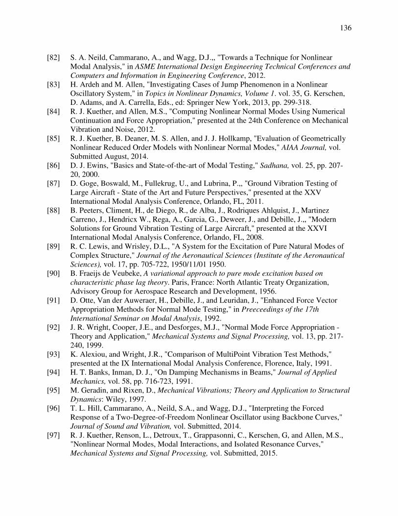
136

[82] S. A. Neild, Cammarano, A., and Wagg, D.J.,, "Towards a Technique for Nonlinear

Modal Analysis," in ASME International Design Engineering Technical Conferences and

Computers and Information in Engineering Conference, 2012.

[83] H. Ardeh and M. Allen, "Investigating Cases of Jump Phenomenon in a Nonlinear

Oscillatory System," in Topics in Nonlinear Dynamics, Volume 1. vol. 35, G. Kerschen,

D. Adams, and A. Carrella, Eds., ed: Springer New York, 2013, pp. 299-318.

[84] R. J. Kuether, and Allen, M.S., "Computing Nonlinear Normal Modes Using Numerical

Continuation and Force Appropriation," presented at the 24th Conference on Mechanical

Vibration and Noise, 2012.

[85] R. J. Kuether, B. Deaner, M. S. Allen, and J. J. Hollkamp, "Evaluation of Geometrically

Nonlinear Reduced Order Models with Nonlinear Normal Modes," AIAA Journal, vol.

Submitted August, 2014.

[86] D. J. Ewins, "Basics and State-of-the-art of Modal Testing," Sadhana, vol. 25, pp. 207-

20, 2000.

[87] D. Goge, Boswald, M., Fullekrug, U., and Lubrina, P.,, "Ground Vibration Testing of

Large Aircraft - State of the Art and Future Perspectives," presented at the XXV

International Modal Analysis Conference, Orlando, FL, 2011.

[88] B. Peeters, Climent, H., de Diego, R., de Alba, J., Rodriques Ahlquist, J., Martinez

Carreno, J., Hendricx W., Rega, A., Garcia, G., Deweer, J., and Debille, J.,, "Modern

Solutions for Ground Vibration Testing of Large Aircraft," presented at the XXVI

International Modal Analysis Conference, Orlando, FL, 2008.

[89] R. C. Lewis, and Wrisley, D.L., "A System for the Excitation of Pure Natural Modes of

Complex Structure," Journal of the Aeronautical Sciences (Institute of the Aeronautical

Sciences), vol. 17, pp. 705-722, 1950/11/01 1950.

[90] B. Fraeijs de Veubeke, A variational approach to pure mode excitation based on

characteristic phase lag theory. Paris, France: North Atlantic Treaty Organization,

Advisory Group for Aerospace Research and Development, 1956.

[91] D. Otte, Van der Auweraer, H., Debille, J., and Leuridan, J., "Enhanced Force Vector

Appropriation Methods for Normal Mode Testing," in Preeceedings of the 17th

International Seminar on Modal Analysis, 1992.

[92] J. R. Wright, Cooper, J.E., and Desforges, M.J., "Normal Mode Force Appropriation -

Theory and Application," Mechanical Systems and Signal Processing, vol. 13, pp. 217-

240, 1999.

[93] K. Alexiou, and Wright, J.R., "Comparison of MultiPoint Vibration Test Methods,"

presented at the IX International Modal Analysis Conference, Florence, Italy, 1991.

[94] H. T. Banks, Inman, D. J., "On Damping Mechanisms in Beams," Journal of Applied

Mechanics, vol. 58, pp. 716-723, 1991.

[95] M. Geradin, and Rixen, D., Mechanical Vibrations; Theory and Application to Structural

Dynamics: Wiley, 1997.

[96] T. L. Hill, Cammarano, A., Neild, S.A., and Wagg, D.J., "Interpreting the Forced

Response of a Two-Degree-of-Freedom Nonlinear Oscillator using Backbone Curves,"

Journal of Sound and Vibration, vol. Submitted, 2014.

[97] R. J. Kuether, Renson, L., Detroux, T., Grappasonni, C., Kerschen, G, and Allen, M.S.,

"Nonlinear Normal Modes, Modal Interactions, and Isolated Resonance Curves,"

Mechanical Systems and Signal Processing, vol. Submitted, 2015.

137

[98] A. A. Muravyov, and Rizzi, S.A., "Determination of Nonlinear Stiffness with Application

to Random Vibration of Geometrically Nonlinear Structures," Computers and Structures,

vol. 81, pp. 1513-1523, 2003.

[99] J. J. Hollkamp and R. W. Gordon, "Reduced-order models for nonlinear response

prediction: Implicit condensation and expansion," Journal of Sound and Vibration, vol.

318, pp. 1139-1153, 2008.

[100] E. J. Breitbach, "A Semi-Automatic Modal Survey Test Technique for Complex Aircraft

and Spacecraft Structures," in Proceedings of 3rd ESA Testing Symposium, 1973, pp.

519-528.

[101] S. W. Shaw, "An Invariant Manifold Approach to Nonlinear Normal Modes of

Oscillation," Journal of Nonlinear Science, vol. 4, pp. 419-448, 1994.

[102] C. Torrence, and Compo, G.P., "A Practical Guide to Wavelet Analysis," Bulletin of the

American Meteorological Society, vol. 79, 1998.

[103] M. Feldman, "Hilbert Transform in Vibration Analysis," Mechanical Systems and Signal

Processing, vol. 25, pp. 735-802, 2011.

[104] L. N. Virgin, Vibration of Axially Loaded Structures. Cambridge, United Kingdom:

Cambridge University Press, 2007.

[105] L. N. Virgin, Introduction to Experimental Nonlinear Dynamics: A Case Study in

Mechanial Vibration. Cambridge, United Kingdom: Cambridge University Press, 2000.

[106] J. D. Schoneman, Allen, M.S., and Kuether, R.J., "Relationships between Nonlinear

Normal Modes and Responses to Random Inputs," presented at the SciTech 2014,

National Harbor, MD, 2014.