Efficient nonlinear modeling of rainfall-runoff process using wavelet compression

Journal of Hydrology (2007) 332, 442–455

ava i lab le at www.sc iencedi rec t . com

journal homepage: www.elsevier .com/ locate / jhydro l

Efficient nonlinear modeling ofrainfall-runoff process using wavelet compression

Chien-ming Chou *

Department of Computer Science and Information Engineering, MingDao University, Changhau 52345, Taiwan, ROC

Received 6 August 2005; received in revised form 31 March 2006; accepted 26 July 2006

Summary This investigation proposes the wavelet-based efficient modeling of nonlinear rain-fall-runoff processes and its application to flood forecasting in a river basin. Inspired by the the-ory of wavelet transforms and Kalman filters, based on the excellent capacity of the Volterramodel, a time-varying nonlinear hydrological model is presented to approximate arbitrary non-linear rainfall-runoff processes. A discrete wavelet transform (DWT) is used to decompose andcompress the Volterra kernels, generating smooth reparametrizations of the Volterra kernels,reducing the number of coefficients to be estimated. Kalman filters were then utilized to on-line estimate compressed wavelet coefficients of the Volterra kernels and thus model thetime-varying nonlinear rainfall-runoff processes. Kalman filters and the Volterra model thathad been used over recent decades in the nonlinear modeling of rainfall-runoff processes,typhoon or storm events over Wu–Tu and Li–Ling watersheds are chosen as case studies wereused herein to verify the suitability of a combination of wavelet transforms. The validationresults indicated that the proposed approach is effective because of the multi-resolution capac-ity of the wavelet transform, the adaptation of the time-varying Kalman filters and the charac-teristics of the Volterra model. Validation results also reveal that the resulting methodimproves the accuracy of the estimate of runoff for small watersheds in Taiwan.ª 2006 Elsevier B.V. All rights reserved.

KEYWORDSWavelet transform;Kalman filter;Volterra model;Rainfall-runoff process;Flood forecasting

0d

Introduction

As Taiwan is located in the major typhoon track in the wes-tern Pacific Ocean, typhoons are an influential weather phe-nomenon in Taiwan, where short, steep upstream channelscharacterize all watersheds. The associated heavy rainfall

022-1694/$ - see front matter ª 2006 Elsevier B.V. All rights reservedoi:10.1016/j.jhydrol.2006.07.015

* Tel.: +886 4 8876660x7400; fax: +886 4 8782134.E-mail address: [email protected].

and flooding are one of the disasters which cause the great-est loss of property and life in the area. It is thereforeessential to study the relationship of the rainfall and runoffprocesses and develop a flood forecasting system to provideprotection and warning systems.

Flood forecasting is based on rainfall-runoff relationshipmodeling. Conventional rainfall-runoff schemes employ a lin-ear time invariant response function to approximate the dy-namic behavior of a rainfall-runoff relationship. Developed

.

mailto:[email protected]

Efficient nonlinear modeling of rainfall-runoff process using wavelet compression 443

by Sherman in 1932, Unit hydrograph (UH) plays a critical rolein predicting runoff hydrograph. However, UH has many lim-itations in application. For instance, linearity and timeinvariance form the basis of UH theory. Despite the extensiveuse of UH, the linear time invariant relationship betweenrainfall and runoff is not strictly valid.

Consequently, the response function with time-varyingcharacteristics, i.e., the ability to adapt to its surroundingenvironment, is necessary. In addition, many nonlinear sys-tems exist. Almost all practical systems, including rainfall-runoff processes, are nonlinear. The modeling of a nonlinearsystem must be studied. Inspired by the theory of wavelettransform and the Kalman filter, and based on the excellentpower of the Volterra model, a time-varying nonlinearhydrologic model is developed for approximating arbitrarynonlinear rainfall-runoff processes herein.

Rainfall-runoff systems are generally non-linear andtime-variant. Their parameters vary in time and space,and when they are assumed constant they are only so byassumption. The inadequacy of the model itself, parameteruncertainty, errors in the data used for parameter estima-tion and inadequate understanding of the rainfall-runoffprocess, owing in part to randomness, may cause errors ina rainfall-runoff model. Incorporating the Kalman filter ina rainfall-runoff model may reduce the error in the runoffprediction arising from the uncertainty caused by the phys-ical process, the model and the input data (Lee and Singh,1998). Lee and Singh also reviewed in detail several applica-tions of the Kalman filter to hydrology.

Identification involves the determination of an unknownsystem based on input–output information in an uncertainenvironment. Volterra filters have been successfully usedin modeling numerous physical applications, especially insignal processing and system identification. The identifica-tion of nonlinear systems depends on an accurate descrip-tion of such. Describing nonlinear systems without ageneral mathematic model is difficult. The Volterra model,which is polynomial (Feng, 1999), can be treated as a gen-eral representation of a nonlinear system. In this paper, anonlinear second-order Volterra model is adopted to modelthe nonlinear rainfall-runoff process. However, the conven-tional method for identifying the Volterra model is ineffi-cient and inaccurate because too many parameters mustbe estimated.

Nikolaou and Mantha (2000) demonstrated how to usewavelets for the reparametrization of second-order Volterramodels in terms of a substantially smaller number of coeffi-cients. The resulting structure retains several of the advan-tages of the Volterra structure, while being parsimonious,thus making feasible the identification of Volterra modelform experimental data. A simulation study on polymeriza-tion reactor elucidates their proposed approach. Herein inthis paper the wavelet transform is similarly applied todecompose and compress the Volterra kernels, and thenKalman filter is adopted to model the nonlinear time-vary-ing rainfall-runoff process.

Wavelets are becoming an increasingly important tool toprocess image and signal. Wavelets effectively extract bothtime and frequency-like information from a time-varyingsignal. Wavelets and Kalman filters can handle the non-stationary signal; many applications combine these twotools. Cheng and Sun (1996) used the theory of wavelet

packet analysis to decompose the primitive measurementsinto two parts, namely the ‘‘trend’’ and ‘‘fluctuation’’ ofthe measurement. Hong et al. (1998) utilize the DWT todecompose the state variables of the Kalman filter into dif-ferent components at the desired resolution level, and thenprocess the prediction, correction and update procedureusing the decomposed state variables.

In the field of hydrology, wavelets have been essentiallyused in order to identify coherent convective storm struc-tures and characterize their temporal variability (Szilagyiet al., 1999) but also in order to explain the non-stationarityof karstic watersheds (Labat et al., 2000). Wavelet analysisof rainfall rates and runoffs and wavelet rainfall-runoffcross-analysis give meaningful information on the temporalvariability of the rainfall-runoff relationship. Wavelets wereregarded as a non-parametric data generation tool proposedby Bayazit and Ahsoy (2001) and applied to annual andmonthly streamflow series taken from Turkey and USA.The idea behind their suggested method is decompositionof data into its details and later reconstruction by summa-tion of the details randomly to generate new data. Chouand Wang (2002) applied the DWT to decompose and com-press the UH. Moreover, a wavelet-based linearly con-strained least mean squares (WLCLMS) algorithm is alsoused to estimate on-line the wavelet coefficients of theUH. Their proposed approach allows the UHs to vary in timeand accurately predicts runoff from a basin, thus making ithighly promising for flood forecasting.

Smith et al. (2004) define a quantitative index that de-scribes the variability in streamflow discharge in terms offiltering of the rainfall signal for an event. They base this in-dex on the interpretation that the wavelet coefficients inthe M · N transform matrix correspond to the correlationbetween the wavelet and the signal. Chou and Wang(2004) proposed a multi-model method using a wavelet-based Kalman filter (WKF) bank to simultaneously estimatedecomposed state variables and unknown parameters forreal-time flood forecasting. Their validations showed thatthe approach is effective because of the decomposition ofwavelet transform, the adaptation of the time-varying KFand the multi-model method properties.

This study is based on the premise that some prior knowl-edge about Volterra kernels can be translated into a sparse-ness pattern of the DWT of the model to be estimated, asproposed by Nikolaou and Mantha (2000). In this investiga-tion, the DWT is first used to transform the original Volterrakernels. A priori information is then used to eliminate sev-eral coefficients by setting them equal to zero. The struc-ture of the original model is retained, and the resultingparsimonious model is simpler to identify. It can be easilyconverted into original form by applying the inverse discretewavelet transform (IDWT). The set of coefficients of theDWT of the Volterra kernels that are set to zero can be iter-atively refined. The Kalman filter algorithm is then used toupdate the compressed wavelet coefficients in each time in-dex, enabling the runoff in the time domain to be predicted.

The rest of this article is organized as follows. First, thestructure of the second-order Volterra models in discrete-time systems is described, after having been identified bythe conventional matrix method in the time domain. Then,the wavelet and the DWT are defined. The decompositionand compression of Volterra models using the DWT is also

444 C.-m. Chou

described, to demonstrate the feasibility of using the wave-let transform to develop parsimonious Volterra kernels andthe resulting modeling approach. Finally, a time-varyingVolterra model using a Kalman filter is introduced. Casestudies of two watersheds in Taiwan are provided to showthe effectiveness of the presented method. Finally, the re-sults are discussed and conclusions drawn.

Nonlinear modeling using Volterra model

The concept of time domain nonlinear Volterrafilter

The Volterra series offers an important general representa-tion of a nonlinear time-invariant system. One benefit ofVolterra filters is that the output y of the systems is linearlyrelated to the Volterra kernels. Accordingly, given the inputand output sequences u and y, the Volterra kernels can bedetermined by solving some linear equations. They can alsobe applied to identify nonlinear systems that are based onthe Volterra filter structure, because the Volterra filtercoefficients are still linearly related to the Volterra output.

Linear models yield fairly good results, so the effect ofnon-linearity in modeling is assumed to be relatively small.Hence, Lattermann (1991) considered that adding only asecond term to the linear hydrological model is adequate.This investigation adopts a second-order Volterra model ofthe nonlinear rainfall-runoff process

yk ¼Xm1

j¼1hðjÞuk�j þ

Xm2

i¼1

Xm2

j¼1gði; jÞuk�iuk�j ¼ y1k þ y2k; ð1Þ

where h(j) and g(i, j) represent the linear and nonlinearparts of second-order Volterra kernels, respectively. m1

and m2 represent the length of data in the linear and nonlin-ear parts of the second-order Volterra kernels, respectively.y1k and y2k represent the Volterra model output generatedby the linear and nonlinear parts of the second-order Vol-terra kernels, respectively.

Identifying second-order Volterra filter in timedomain

Assume that the system to be identified has the followingdiscrete convolution structure for (Nikolaou and Mantha,2000);

yk ¼ y1k þ y2k þ ek

¼Xm1

j¼1hðjÞuk�j þ

Xm2

i¼1

Xm2

j¼1gði; jÞuk�iuk�j þ ek

¼ uT1khþ uT

2kGu2k þ ek; ð2Þ

where u1k ¼ ½uk�1 � � � uk�m1�T, u2k ¼ ½uk�1 � � � uk�m2

�T and ek isthe output-additive random noise with zero mean. The fol-lowing analysis does not require that m1 =m2. The kernelcoefficient matrix G in the double sum in Eq. (2) can be as-sumed to be symmetric without loss of generality, suggest-ing that of the m2

2 second-order coefficients, onlyM2 = m2(m2 + 1)/2 coefficients are distinguishable. For nota-tional consistency, M1 = m1 is defined to be the number ofdistinct linear coefficients.

The vector vecl t(G) contains all the distinct elements ofG: all elements in the lower-triangular part of G, and y2k canbe written as (Nikolaou and Mantha, 2000),

y2k ¼ uT2kltXglt; ð3Þ

where u2kltX ¼ Xm2vecltðU2kÞ, U2k ¼ u2kuT

2k, glt = veclt(G),and

Xm2¼ diag 1; 2; 2; . . . 2|fflfflfflfflfflfflffl{zfflfflfflfflfflfflffl}

m2 elements

1; 2; 2; . . . 2|fflfflfflfflfflfflffl{zfflfflfflfflfflfflffl}m2�1 elements

� � � 1|{z}1 elements

0B@1CA:

Therefore, the entire Volterra model as Eq. (2) can beparameterized in the standard linear regression form as(Nikolaou and Mantha, 2000)

yk ¼ /Tkhþ ek; ð4Þ

where /k ¼ ½u1k

u2kltX� and h ¼ ½ h

glt�. The ordinary least squares

(OLS) method (Takahashi et al., 1998) can be used to yieldparameter h.

Wavelet theory

Wavelet analysis

The definitions of wavelets used herein were taken from Raoand Bopardikar (1998) and Bayazit and Ahsoy (2001), and arepresented herein for convenience. The definitions are as fol-lows: A wavelet w(t) is a function with the following proper-ties (Rao and Bopardikar, 1998):

(I) The function integrates to zero:Z 1

�1wðtÞ dt ¼ 0: ð5Þ

(II) The function is square integrable or, equivalently, hasfinite energy:Z 1

�1jwðtÞj2 dt <1: ð6Þ

In this paper, the wavelet used for analysis herein is thequadratic spline (QS) wavelet, which belongs to the Battle–Lemarie group (Zhang et al., 2002). The QS-wavelet has onlyone vanishing moment (Ge and Mirchandani, 2003). The sim-plest filters correspond to the Haar wavelet, which has theadvantage of orthogonality (selfduality), but it has poor fil-tering characteristics. To obtain good quality of compres-sion and recovery during the procedure of signalcompression, orthogonal wavelet base is usually beingsubstituted for biorthogonal wavelet base (Wang and Yang,2004). The main reasons for our choice are the biorthogo-nality of the QS-wavelet and its dual, and good interpolationproperties (Zhang et al., 2002).

One-dimensional DWT (1-D DWT)

The 1-D and 2-D DWTs are applied to the decomposition andcompression of the Volterra model. The definitions of wave-let decomposition used herein were taken from Nikolaouand Mantha (2000), and are presented herein forconvenience.


Vectors hj and ij with dimensions 2j · 1 (0 6 j 6 r � 1)are able to be obtained recursively by linearly transformingmatrix Fj with dimensions 2j · 2j. Each step in the recursivealgorithm is one of single-step discrete wavelet decomposi-tion (Nikolaou and Mantha, 2000):

½ðhj�1ÞT ðij�1ÞT�T ¼ Fjhj; j ¼ 1; 2; . . . ; r; ð7Þ

Fj¼½CTj DT

j �T; ð8Þ

where Cj and Dj are matrices of dimensions 2j�1 · 2j, whichcan be determined by filtering the vector hj through a low-pass filter C and a high-pass filter D that are associated withthe primal wavelet, respectively. Herein the primal waveletis the QS-wavelet used in this paper. The dual wavelet rep-resents the inverse of the primal wavelet.

The coefficients of filters C and D in the QS-wavelet aredefined as follows (Nikolaou and Mantha, 2000):

Cj ¼

c0 þ c1 c2 c3

c0 c1 c2 c3

c0 c1 c2 c3

. .. . .

. . ..

c0 c1 c2 þ c3

266666664

377777775; ð9Þ

Dj ¼

d0 þ d1 d2 d3

d0 d1 d2 d3

d0 d1 d2 d3

. .. . .

. . ..

d0 d1 d2 þ d3

266666664

377777775; ð10Þ

where

ðc0 c1 c2 c3Þ ¼1

2ffiffiffi2p ð�1 3 3 � 1Þ; ð11Þ

ðd0 d1 d2 d3Þ ¼1

2ffiffiffi2p ð�1 3 � 3 1Þ: ð12Þ

For the computation of the inverse DWT (IDWT), we needthe corresponding reconstruction lowpass filter eC andreconstruction highpass filter eD associated with the dualwavelet (Nikolaou and Mantha, 2000). The two waveletsare biorthogonal (Strang and Nguyen, 1996). Similarly, fil-ters eC and eD can be defined by substituting coefficientsc0, c1, c2, c3, d0, d1, d2 and d3 in filters C and D using coef-ficients ~c0, ~c1, ~c2, ~c3, ~d0, ~d1, ~d2 and ~d3, respectively, as fol-lows (Nikolaou and Mantha, 2000).

ð~c0 ~c1 ~c2 ~c3Þ ¼1

2ffiffiffi2p ð1 3 3 1Þ; ð13Þ

ð~d0~d1

~d2~d3Þ ¼

1

2ffiffiffi2p ð1 3 � 3 � 1Þ: ð14Þ

The vector h, which is in the time domain, needs to bedecomposed. The 1-D DWT of h, with respect to (w.r.t)the primal wavelet, is then obtained by linear transforma-tion (Nikolaou and Mantha, 2000):

g ¼ W1h; ð15Þ

where W1 = N1N2. . .Nr,

Nj ¼Fj 0

0 I

� �; j ¼ 1; 2; . . . ; r:

The 1-D DWT of h with respect to the dual wavelet can beobtained in a similar manner (Nikolaou and Mantha, 2000):

~g ¼ fW 1h: ð16Þ

The duration L of vector h is assumed to be an integralpower of 2, L = 2r. The orthogonal condition yields,eFT

j Fj ¼ I2j ; j ¼ 1; 2; . . . ; r) fWT1W1 ¼ I2r : ð17Þ

Two-dimensional DWT (2-D DWT)

As Volterra kernels consist of a linear part (1-D) and a nonlin-ear part (2-D), 1-D and 2-D DWTs were applied to transformthe linear and the nonlinear part of Volterra kernels, respec-tively. The 2-D DWT of a matrix is obtained by a transforma-tion that generates a new matrix of the same dimensions asthe original matrix. The transformation is such that eachelement in the 2-D DWT is a linear combination of the ele-ments in the original matrix. Only the classes of 2-D waveletsthat are biorthogonal and are a separable multi-resolutionanalysis (MRA) approximation of R2 are considered. Biorthog-onality is used to prevent inefficient numerical inversion ofthe DWT transformation matrix (W1 or W2) during the com-putation of the IDWT. Separability provides two advantagesthat facilitate analysis. First, 2-D filtering using wavelet fil-ters may be performed as two successive 1-D filterings. Sec-ond, the 2-D DWT of the symmetric matrix G is alsosymmetric, so the unknown parameters to be identifiedare in the same form in both the kernel and its 2-D DWT. Ow-ing to considerations of space. A detailed description of the2-D DWT is presented in Nikolaou and Mantha (2000).

Compression of Volterra kernels using DWT

Decomposition and compression of Volterra kernelsusing DWT

In this paper, the linear and nonlinear part of a second-or-der Volterra kernel can be decomposed and compressedusing 1-D and 2-D DWT, respectively. Applying 1-D DWT todecompose and compress hydrological series can be foundin Chou and Wang (2004), because of spatial constraints.The nonlinear part of a second-order Volterra kernel maybe treated like Nikolaou and Mantha (2000). However, thealgebra is more involved and presented here only in brief.Details are presented in Nikolaou and Mantha (2000). Sup-pose that the 2-D DWT of the nonlinear part of kernel G isC. G is symmetric, so C is also symmetric. Define the vec-tor-valued function ‘veclt’ of an (m · m) square matrix Qas the (m(m + 1)/2 · 1) vector (Nikolaou and Mantha, 2000)

vecltðQÞ ¼ q11 � � � qm21|fflfflfflfflfflfflffl{zfflfflfflfflfflfflffl} q22 � � � qm22|fflfflfflfflfflfflffl{zfflfflfflfflfflfflffl} � � � qm2m2|fflffl{zfflffl}� �T

ð18Þ

obtained by considering the lower triangular part of Q andstacking the columns (of declining length) in a vector.Hence, the vector (Nikolaou and Mantha, 2000)

446 C.-m. Chou

clt ¼ vecltðCÞ ð19Þ

comprises all of the distinct elements in C, and the outputof the nonlinear part of the second-order Volterra kernelis shown to be (Nikolaou and Mantha, 2000)

y2k ¼ ~vT2kltXclt; ð20Þ

where the vector ~vT2ltXðkÞ is a corresponding transformation

of the input vector u2(k), which involves the 2-D DWT w.r.t.the dual wavelet.

Model compression using wavelets first involves deter-mining the DWT coefficients of the kernel. Of the obtainedDWT coefficients, only the coefficients with magnitudeabove a certain threshold value are retained, the rest beingassumed to be zero (Nikolaou and Vuthandam, 1998). Here-in, when only Mc2 6 M2 elements of the total of M2 elementsof clt are significant, clt can be compressed to the vector(Nikolaou and Mantha, 2000)

cltc ¼ Pc2clt; ð21Þ

analogously to the compression in the linear-kernel case,where the matrix Pc2 selects the desired elements of thematrix clt. The transformed input vector is correspondinglycompressed to the vector (Nikolaou and Mantha, 2000)

~vT2kltXc ¼ Pc2~vT

2kltX: ð22Þ

The nonlinear part of the second-order Volterra term inthe output is now approximated as

y2k � ½~vT2kltXc�

Tcltc: ð23Þ

Again, given the compressed 2-D DWT cltc, the discrete-timenonlinear part of the second-order Volterra kernel Gc can bereconstructed using the transformation (Nikolaou and Man-tha, 2000),

vecðGcÞ ¼ X2cltc; ð24Þ

where the matrix X2 involves a 2-D IDWT.

Identifying second-order Volterra kernel usingwavelet compression

Some of the coefficients of DWTs g and clt of kernels h (lin-ear part) and glt (nonlinear part), respectively, to be identi-fied are assumed to be identically zero. Then, the fullVolterra model of the equation can be approximated as(Nikolaou and Mantha, 2000),

yk ¼ y1k þ y2k þ ek � /Tkchc þ ek; ð25Þ

where

/kc ¼~v1kc

~vT2kltXc

� �and hc ¼

gc

cltc

� �:

~v1kc and ~vT2kltXc represent the compressed DWTs of the in-

put vectors w.r.t the dual wavelet for linear part and non-linear part of second-order Volterra kernels, respectively.gc and cltc represent the compressed coefficients of DWTsg and clt, respectively. This model is similar to a linearequation. However, a much shorter vector hc of length(Mc1 + Mc2) in the wavelet domain is now identified, ratherthan vector h of length (M1 + M2) in the time domain. WithN observations, yielding the outputs (Nikolaou and Man-tha, 2000),

y ¼ UTchc þ e; ð26Þ

where UTc ¼ ½/ðk�Nþ1Þc � � �/kc�. The compressed discrete-time

domain kernels can be obtained from the standard least-squares estimate of the parameter vector hc as (Nikolaouand Mantha, 2000),

hc

vecðGcÞ

" #¼

X1gc

X2cltc

� �¼

X1 0

0 X2

� �hc: ð27Þ

Selecting which coefficients in g and clt that are set tozero is crucial to identify accurately the Volterra model. Iftoo many coefficients are set to zero, then the approximateVolterra model will be inaccurate. If too few coefficientsare zeroed, then the resulting estimator will have high var-iance caused by overparametrization. Therefore, the coeffi-cients that must be set to zero have to be selectediteratively, by applying thresholding and standard good-ness-of-fit criteria in each iteration. Prior knowledge ofthe dynamic behavior of a modeled plant can yield usefulguidelines regarding which coefficients should be set to zeroat the beginning of the iterative procedure (Nikolaou andMantha, 2000).

The way of thresholding in this paper was taken fromNikolaou and Vuthandam (1998) and revised as shownbelow:

Step 1 Let resolution level l for linear part and nonlinearpart of second-order Volterra model be 5 and 4,respectively, according to the length of kernels.Obtain the DWT of the prior Volterra model. Obtaina set of indices for detail coefficients to retain,according to certain thresholds.

Step 2 Identify the DWT coefficients corresponding toretained indices using observed rainfall-runoffdata. Construct Volterra model.

Step 3 Perform tests on the prediction residuals based onthe criteria of EV, CE, EQp and ETp.

Step 4 If the residuals test satisfactorily then go to step 6,otherwise continue.

Step 5 Adjust thresholds. Add/Drop DWT details accordingto adjusted thresholds, and repeat steps 2–4.

Step 6 Stop.

Time-varying Volterra model that incorporateswavelet compression and Kalman filter

Kalman filter

The Kalman filter, a linear dynamic system, imitates thebehavior of an observed natural process. The Kalman filteraccomplishes this by optimally estimating the current stateof the observed process at each instant. This state estimateis coupled with an internal model of the observed process topredict the next output. When the next output occurs, thefilter calculates the difference between its prediction andthe actual output, and uses this residual to adjust (or up-date) its estimate of the state. The new corrected estimatecan then predict the next state, thus completing one fulliteration of the filter. In this study, the adaptive Kalman fil-ter was applied to determine covariance matrices Qk and Rk


corresponding to system noise and measurements noise,respectively. The detail could be found in Chou and Wang(2004).

Application of Kalman filter to compressednonlinear volterra model

A Kalman filter was adopted in a compressed second-orderVolterra model to elucidate the time-variation of nonlinearrainfall-runoff process. Then, the wavelet coefficients ofthe Volterra kernel can be predicted, corrected and up-dated. The state equation is

hðkþ1Þc ¼gðkþ1Þccðkþ1Þltc

" #¼

gkc

ckltc

� �þ wk: ð28Þ

The observation equation is

yk ¼ /Tkchkc þ vk; ð29Þ

where

/kc ¼~v1kc

~vT2kltXc

� �; hkc ¼

gkc

ckltc

� �:

Application and analysis

Study basin

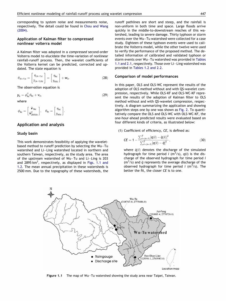
This work demonstrates feasibility of applying the wavelet-based method to runoff prediction by selecting the Wu–Tuwatershed and Li–Ling watershed located in northern andsouthern Taiwan, respectively, as the study area. The areaof the upstream watershed of Wu–Tu and Li–Ling is 203and 2895 km2, respectively, as displayed in Figs. 1.1 and1.2. The mean annual precipitation in these watersheds is2500 mm. Due to the topography of these watersheds, the

Figure 1.1 The map of Wu–Tu watershed sh

runoff pathlines are short and steep, and the rainfall isnon-uniform in both time and space. Large floods arrivequickly in the middle-to-downstream reaches of this wa-tershed, leading to severe damage. Thirty typhoon or stormevents over the Wu–Tu watershed were collected for a casestudy. Eighteen of these typhoon events were used to cali-brate the Volterra model, while the other twelve were usedto verify the performance of the proposed method. The de-tailed information of calibrated and validated typhoon orstorm events over Wu–Tu watershed was provided in Tables1.1 and 2.1, respectively. Those over Li–Ling watershed wasprovided in Tables 1.2 and 2.2.

Comparison of model performances

In this paper, OLS and OLS-WC represent the results of theadoption of OLS method without and with QS-wavelet com-pression, respectively. While OLS-KF and OLS-WC-KF repre-sent the results of the adoption of Kalman filter to OLSmethod without and with QS-wavelet compression, respec-tively. A diagram summarizing the application and showingalgorithm steps one by one was shown as Fig. 2. To quanti-tatively compare the OLS and OLS-WC with OLS-WC-KF, theone-hour-ahead predicted results were evaluated based onfour different kinds of criteria, as illustrated below:

(1) Coefficient of efficiency, CE, is defined as:

CE ¼ 1�PT

i¼ðnþ1Þ½qðiÞ � qðiÞ�2PTi¼ðnþ1Þ½qðiÞ � �q�2

; ð30Þ

where qðiÞ denotes the discharge of the simulatedhydrograph for time period i (m3/s), q(i) is the dis-charge of the observed hydrograph for time period i(m3/s) and �q represents the average discharge of theobserved hydrograph for time period i (m3/s). Thebetter the fit, the closer CE is to one.

owing the study area near Taipei, Taiwan.

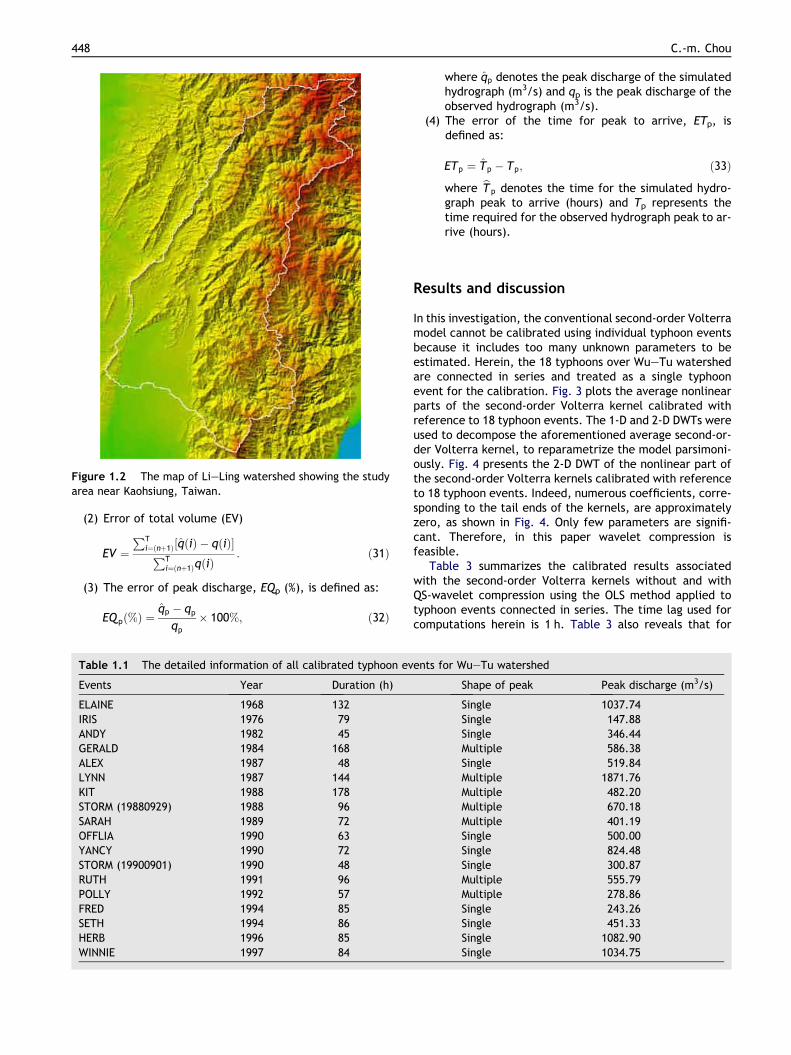
Figure 1.2 The map of Li–Ling watershed showing the studyarea near Kaohsiung, Taiwan.

448 C.-m. Chou

(2) Error of total volume (EV)

EV ¼PT

i¼ðnþ1Þ½qðiÞ � qðiÞ�PTi¼ðnþ1ÞqðiÞ

: ð31Þ

(3) The error of peak discharge, EQp (%), is defined as:

EQ pð%Þ ¼qp � qp

qp

� 100%; ð32Þ

Table 1.1 The detailed information of all calibrated typhoon ev

Events Year Duration (h)

ELAINE 1968 132IRIS 1976 79ANDY 1982 45GERALD 1984 168ALEX 1987 48LYNN 1987 144KIT 1988 178STORM (19880929) 1988 96SARAH 1989 72OFFLIA 1990 63YANCY 1990 72STORM (19900901) 1990 48RUTH 1991 96POLLY 1992 57FRED 1994 85SETH 1994 86HERB 1996 85WINNIE 1997 84

where qp denotes the peak discharge of the simulatedhydrograph (m3/s) and qp is the peak discharge of theobserved hydrograph (m3/s).

(4) The error of the time for peak to arrive, ETp, isdefined as:

ETp ¼ Tp � Tp; ð33Þ

where bT p denotes the time for the simulated hydro-graph peak to arrive (hours) and Tp represents thetime required for the observed hydrograph peak to ar-rive (hours).

Results and discussion

In this investigation, the conventional second-order Volterramodel cannot be calibrated using individual typhoon eventsbecause it includes too many unknown parameters to beestimated. Herein, the 18 typhoons over Wu–Tu watershedare connected in series and treated as a single typhoonevent for the calibration. Fig. 3 plots the average nonlinearparts of the second-order Volterra kernel calibrated withreference to 18 typhoon events. The 1-D and 2-D DWTs wereused to decompose the aforementioned average second-or-der Volterra kernel, to reparametrize the model parsimoni-ously. Fig. 4 presents the 2-D DWT of the nonlinear part ofthe second-order Volterra kernels calibrated with referenceto 18 typhoon events. Indeed, numerous coefficients, corre-sponding to the tail ends of the kernels, are approximatelyzero, as shown in Fig. 4. Only few parameters are signifi-cant. Therefore, in this paper wavelet compression isfeasible.

Table 3 summarizes the calibrated results associatedwith the second-order Volterra kernels without and withQS-wavelet compression using the OLS method applied totyphoon events connected in series. The time lag used forcomputations herein is 1 h. Table 3 also reveals that for

ents for Wu–Tu watershed

Shape of peak Peak discharge (m3/s)

Single 1037.74Single 147.88Single 346.44Multiple 586.38Single 519.84Multiple 1871.76Multiple 482.20Multiple 670.18Multiple 401.19Single 500.00Single 824.48Single 300.87Multiple 555.79Multiple 278.86Single 243.26Single 451.33Single 1082.90Single 1034.75

Table 1.2 The detailed information of all calibrated typhoon events for Li–Ling watershed

Events Year Duration (h) Shape of peak Peak discharge (m3/s)

STORM (19950608) 1995 144 Single 1710.81GLORIA 1996 72 Multiple 3008.86STORM (19970701) 1997 72 Single 2073.45STORM (19970829) 1997 72 Multiple 720.82


Wu–Tu watershed the numbers of parameters in the originallinear and nonlinear parts are 32 and 136, respectively. Fol-lowing QS-wavelet compression, the numbers of parametersare estimated to be only 5 and 39, respectively. Fig. 5 dis-plays the linear parts of the calibrated second-order Vol-terra kernels using OLS without and with QS-waveletcompression for all typhoon events. It also demonstratesthat QS-wavelet compression yields a smoother kernel.

Fig. 6 depicts the nonlinear parts of calibrated second-order Volterra kernels using OLS with QS-wavelet compres-sion for all typhoon events. Fig. 7 presents the calibrationresults obtained from the second-order Volterra model

Effectrainfall

Calibrating usingVolterra model in

time domain

Wavel& co

CalibVoltewave

Wavelet transform& compression

The results obtainedusing OLS

The resusing

Validating usingVolterra model in

time domain

ValidVoltewave

Direct runoff

Figure 2 The diagram sum

using OLS without and with QS-wavelet compression for alltyphoon events. Comparing Fig. 3 with Fig. 6, it is shownthat with a little lost of accuracy in the prediction the non-linear part of second-order Volterra kernels with QS-wave-let compression is smoother than that without QS-waveletcompression. The number of parameters to be estimateddeclines, so the nonlinear rainfall-runoff process can beefficiently modeled.

Table 4 quantitatively compares these four methods withreference to four selected model efficiency criteria. Thevalidation results demonstrate that the CE for theOLS-WC-KF (with an average value of 0.939) exceeds that

et transformmpression

rating usingrra model inlet domain

ults obtained OLS-WC

The results obtainedusing OLS-WC-KF

Kalman filter

ating usingrra model inlet domain

Regarding validatedwavelet domain

Volterra model asinitial value

marizing the application.

Figure 3 The average nonlinear part of the second-orderVolterra kernel calibrated with reference to 18 typhoon eventsfor Wu–Tu watershed.

Figure 4 The 2-D DWT of the nonlinear part of the second-order Volterra kernels calibrated with reference to 18 typhoonevents for Wu–Tu watershed.

Table 2.1 The detailed information of all validated typhoon eve

Events Year Duration (h)

NADINE 1968 50ELSIE 1969 60BESS 1971 66STORM (19771115) 1977 96FREDA 1984 59STORM (19850208) 1985 72ABBY 1986 118STORM (19910922) 1991 53DOUG 1994 67GLADYS 1994 96ZANE 1996 112AMBER 1997 71

450 C.-m. Chou

for the OLS-WC (with an average value of 0.921), and thatthe CE for the OLS-WC-KF (with an average value of 0.939)significantly exceeds that of the OLS (with an average valueof 0.898). According to the EV criteria, the OLS-WC and OLSperform slightly better than the OLS-WC-KF. In flood fore-casting, the prediction of the peak discharge is very impor-tant for protection and flood warning systems. According tothe EQp criteria, the average value for OLS and OLS-WC is17.15% and 11.01%, respectively. The developed OLS-WC-KF brings real improvement (with an average value of7.37%) to the peak discharge, which is important informa-tion from practical point of view.

The results using Kalman filter but no wavelet compres-sion were compared with that of other modelings and in-cluded in Table 4. In this study, OLS-KF is the special caseof OLS-WC-KF in which the threshold values equal to 0.The results demonstrate that although OLS-KF outperformlightly OLS-WC-KF based the criteria of CE. OLS-WC-KF canobtain the better results than OLS-KF, based the criteriaof EV and EQp. The results also demonstrate that OLS-KFhas a little loss of accuracy in the prediction due to thattoo many parameters must be estimated.

Figs. 8 and 9 show two representative sets of validationresults, based on the calibrated results in Figs. 5 and 6.Overall, the validation results indicate that the approachwith QS-wavelet compression outperforms that withoutQS-wavelet compression. Overfitting occurs in the methodwithout QS-wavelet compression, meaning that too manyparameters must to be estimated from finite observed data.Wavelet compression reduces the number of parameters tobe estimated, preventing overfitting. Hence, wavelet com-pression generates smoother kernels, to yield better valida-tion results. The validation results also demonstrate thatthe incorporation of a Kalman filter in the nonlinear Volterramodel with QS-wavelet causes this model to outperformthat without such a Kalman filter. The Kalman filter can pre-dict, correct and update fewer parameters (compressedwavelet coefficients), so the rainfall-runoff process can beprecisely modeled.

The difference between excellent and poor forecastcases may be due to the proposed method applied in this pa-per, which is lumped model. Lumped models are models inwhich the parameters do not vary spatially over the entirewatershed. The assumption of uniform distributed rainfall

nts for Wu–Tu watershed

Shape of peak Peak discharge (m3/s)

Single 219.67Single 662.54Single 994.12Single 538.39Single 501.45Multiple 235.91Multiple 579.01Single 89.89Multiple 320.07Single 434.24Multiple 665.98Single 953.51

Table 2.2 The detailed information of all validated typhoon events for Li–Ling watershed

Events Year Duration (h) Shape of peak Peak discharge (m3/s)

TIM 1994 72 Multiple 3184.32STROM(19980804) 1998 72 Multiple 1804.47ZEB 1998 72 Multiple 2068.80

Table 3 The calibrated results associated with the second-order Volterra kernels without and with QS-wavelet compressionusing the OLS method applied to typhoon events connected in series

Events Datalength

1-D retainednumberfrom 32

2-D retainednumberfrom 136

EV (%) CE EQp (%) ETp (h)

OLS OLS-WC OLS OLS-WC OLS OLS -WC OLS OLS-WC

In seriesWu–Tu

1638 5 39 2.23 2.30 0.948 0.915 �1.16 �8.82 �1 0

In seriesLi–Ling

360 17 73 4.35 4.32 0.824 0.805 �4.78 �5.41 0 0

Note: The unit of data length is hours.

0 2 4 6 8 10 12 14 16 18 20 22 24 26 28 30 32

Time (hours)

-0.02

0.00

0.02

0.04

0.06

0.08

0.10

Sec

ond

orde

r V

olte

rra

kern

el (

1/ho

ur) ALL EVENTS

OLS

OLS-WC

Figure 5 The linear parts of the calibrated second-orderVolterra kernels using OLS without and with QS-waveletcompression for all typhoon events for Wu–Tu watershed.

Figure 6 The nonlinear parts of calibrated second-orderVolterra kernels using OLS with QS-wavelet compression for alltyphoon events for Wu–Tu watershed.


may affect the performance of the proposed method. Inaddition, the rainfall centers on upstream or downstreamof the watershed, which may also affect the performance ofthe proposed method. For example, based on the criteria ofCE, in the STORM (19910922) with the lowest value 0.839,the rainfall duration is very short (e.g. 5 h) and intermit-tent. According to this input rainfall, this method producespoor runoff estimation or forecast. In contrast, based on thecriteria of CE, in the Typhoon NADINE with the highest value0.980, the rainfall duration is 11 h and successive, the meth-od producing excellent runoff estimation or forecast.

To illustrate the proposed methodology work for differ-ent watersheds, the Li–Ling watershed located in southernTaiwan with 2895 km2 was chosen. The validation resultsare shown as Figs. 10, 11 and Table 5. These results dem-onstrate that the performance of the proposed method in

the Li–Ling watershed does not outperform that in theWu–Tu watershed. From the comparison between the val-idation results of the Wu–Tu and the Li–Ling watershed, itappears that the proposed nonlinear time-varying methodis more suitable for small watersheds than big watersheds.It was previously shown that the bigger the area of wa-tershed is, the slighter nonlinearity the watershed has(Rui, 2004).

The comparison between one-hour and six-hour lead-time forecasts for Wu–Tu watershed is shown as Table 6.The results of six-hour lead-time forecasts is less precisethan that of one-hour lead-time forecasts, due to the accu-mulated errors. The CE for six-hour lead-time forecasts(with an average value of 0.843) illustrates that six-hourlead-time forecasts could provide available information inthe flood forecasting.

Table 4 The results of validation for Wu–Tu watershed

Events Year EV (%)

OLS OLS-WC OLS-KF O

NADINE 1968 5.14 2.43 �2.05ELSIE 1969 4.17 5.98 7.68BESS 1971 3.06 3.83 �1.20STORM (19771115) 1977 �0.69 1.19 4.84FREDA 1984 �0.92 5.39 0.62STORM (19850208) 1985 1.14 0.52 2.09ABBY 1986 �2.56 1.77 �1.86STORM (19910922) 1991 �3.10 �0.15 �3.15DOUG 1994 5.66 3.92 5.24GLADYS 1994 3.69 �0.26 8.85ZANE 1996 �1.83 0.86 7.27AMBER 1997 �1.68 1.79 �2.95

Average 2.80 2.34 3.98

EQp (%)

OLS OLS-WC OLS-KF O

NADINE 1968 0.88 �4.01 15.33ELSIE 1969 10.18 �3.28 17.64BESS 1971 �1.52 �19.82 8.63STORM (19771115) 1977 5.78 �4.39 4.34FREDA 1984 �16.42 �11.67 4.90STORM (19850208) 1985 19.71 3.55 5.70ABBY 1986 21.23 14.75 51.32STORM (19910922) 1991 33.90 19.38 26.54DOUG 1994 �26.29 �21.99 �15.15 �GLADYS 1994 43.24 2.68 16.62ZANE 1996 13.96 �4.55 8.83AMBER 1997 �12.67 �22.02 7.06

Average 17.15 11.01 15.17

Note: The columns for EV, EQp and ETp all contain negative values, an

0 200 400 600 800 1000 1200 1400 1600

Time (hours)

0100200300400500600700800900

1000110012001300140015001600170018001900

Dis

char

ge (

cms)

0 200 400 600 800 1000 1200 1400 16000

10

20

30

40

50Rai

nfal

l (m

m/h

r)

ALL EVENTS

Obs. discharge

Est. discharge (OLS)

Est. discharge (OLS-WC)

Figure 7 The calibration results obtained from the second-order Volterra model using OLS without and with QS-waveletcompression for all typhoon events for Wu–Tu watershed.

452 C.-m. Chou

The proposed lumped non-linear time-varying method re-lies on rainfall observations and changes significantly withthe rainfall, such as the type of storm, rainfall intensityand duration. When the type of storm is intermittent, theestimated runoff hydrograph shows unevenly, as shown inFigs. 9–11. In contrast, when the type of storm is succes-sive, the estimated runoff hydrograph shows smoothly, asshown in Fig. 8. The bigger the rainfall intensity is, the thin-ner and more concentrative the estimated runoff hydro-graph will be. For example, the estimated runoffhydrograph in Fig. 9 is thinner and more concentrative thanthat in Fig. 8. In addition, the bigger the rainfall intensity is,the earlier the time to peak appears.

The data length of the linear and nonlinear parts of thesecond-order kernels is chosen to be 32 and 16, respec-tively. The length of the nonlinear parts of the second-or-der kernels need not equal that of the linear parts. If toomany parameters must be estimated, then the OLS meth-od may not be applied efficiently. Furthermore, numerouscoefficients that correspond to the tail ends of the kernelshave values of approximately zero, so the length of thenonlinear parts of the second-order kernels is set to24 = 16, based on the characteristics of the wavelettransform.

CE

LS-WC-KF OLS OLS-WC OLS-KF OLS-WC-KF

1.68 0.981 0.979 0.952 0.9809.87 0.931 0.927 0.915 0.9170.07 0.938 0.916 0.905 0.9651.46 0.932 0.936 0.979 0.9594.46 0.884 0.963 0.959 0.9682.29 0.876 0.932 0.917 0.9381.31 0.912 0.928 0.897 0.9433.55 0.704 0.819 0.745 0.8393.51 0.897 0.906 0.926 0.9234.67 0.869 0.907 0.910 0.9461.90 0.911 0.938 0.940 0.9571.57 0.940 0.896 0.954 0.933

3.03 0.898 0.921 0.917 0.939

ETp (h)

LS-WC-KF OLS OLS-WC OLS-KF OLS-WC-KF

�2.21 0 0 0 01.39 0 1 0 0�1.29 1 1 �1 �13.68 �2 0 0 0�7.29 1 0 1 05.29 �2 0 0 0

12.43 2 4 10 323.72 �3 �3 �3 �418.60 �2 0 1 29.98 �1 �1 0 �1�0.80 �1 �1 1 0�1.80 0 0 0 0

7.37 1.25 0.92 0.92 0.92

d these columns present the averages of the absolute values.

0 10 20 30 40 50 60 70 80 90 100

Time (hours)

0

100

200

300

400

500

600

Dis

char

ge (

cms)

0 10 20 30 40 50 60 70 80 90 100

0

10

20Rai

nfal

l (m

m/h

r)

STORM1977.11.15

Obs. discharge



Est. discharge (OLS-WC-KF)

Figure 8 The validation results for Wu–Tu watershed, basedon the calibrated results in Figs. 5 and 6, for STORM (19771115),1977.

0 10 20 30 40 50 60 70 80 90 100 110 120

Time (hours)

0

100

200

300

400

500

600

700

800

Dis

char

ge (

cms)

0 10 20 30 40 50 60 70 80 90 100 110 1200

10

20

30Rai

nfal

l (m

m/h

r)

ZANE1996.09.27

Obs. discharge




Figure 9 The validation results for Wu–Tu watershed, basedon the calibrated results in Figs. 5 and 6, for Typhoon ZANE,1996.

0 10 20 30 40 50 60 70 80

Time (hours)

0

500

1000

1500

2000

2500

Dis

char

ge (

cms)

0 10 20 30 40 50 60 70 80

0

10Rai

nfal

l (m

m/h

r)

ZEB1998.10.15

Obs. discharge




Figure 11 The validation results for Li–Ling watershed forTyphoon ZEB, 1998.

0 10 20 30 40 50 60 70 80

Time (hours)

0

500

1000

1500

2000

2500

3000

3500

4000

4500

Dis

char

ge (

cms)

0 10 20 30 40 50 60 70 80

0

10

20Rai

nfal

l (m

m/h

r)

TIM1994.07.11

Obs. discharge




Figure 10 The validation results for Li–Ling watershed forTyphoon TIM, 1994.


Conclusions

This investigation used the wavelet transform, which cancapture the features of signals, to decompose and compresssecond-order Volterra kernels efficiently. QS-wavelet com-pression yields smoother kernels. A Kalman filter predictsfewer wavelet coefficients, which have significant values,

so can be used effectively to model a nonlinear time-varyingrainfall-runoff process.

Wavelet compression reduces the 32 + 136 = 168 esti-mated parameters of the original second-order Volterramod-el to 5 + 39 = 44. If too many parameters must be estimatedfrom finite observed data, then overfitting occurs. Waveletcompression eliminates overfitting. Wavelet compressioncan capture and retain the characteristics of signals, simplify-ing the estimation of parameters.

Table 5 The results of validation for Li–Ling watershed

Events Year EV (%) CE

OLS OLS-WC OLS-KF OLS-WC-KF OLS OLS-WC OLS-KF OLS-WC-KF

TIM 1994 �5.32 �5.34 0.50 0.38 0.809 0.814 0.890 0.891STROM (19980804) 1998 �5.34 �5.71 2.76 2.88 0.724 0.725 0.791 0.788ZEB 1998 �5.22 �5.68 1.23 0.91 0.800 0.799 0.836 0.841

Average 5.30 5.58 1.50 1.39 0.778 0.779 0.839 0.840

EQP (%) ETp (h)

OLS OLS-WC OLS-KF OLS-WC-KF OLS OLS-WC OLS-KF OLS-WC-KF

TIM 1994 29.40 29.14 34.04 35.19 �11 �11 �11 �11STROM (19980804) 1998 �14.04 �13.76 3.34 7.64 2 2 7 7ZEB 1998 10.10 10.50 4.06 4.09 �1 �1 1 1

Average 17.85 17.80 13.81 16.64 4.67 4.67 6.33 6.33

Note: The columns for EV, EQp and ETp all contain negative values, and these columns present the averages of the absolute values.

Table 6 The comparison between one-hour and six-hour lead-time forecasts for Wu–Tu watershed

Events Year EV (%) CE EQp (%) ETp(h)

1-hour 6-hour 1-hour 6-hour 1-hour 6-hour 1-hour 6-hour

NADINE 1968 1.68 �2.37 0.980 0.873 �2.21 19.87 0 0ELSIE 1969 9.87 �3.61 0.917 0.864 1.39 35.07 0 0BESS 1971 0.07 12.12 0.965 0.820 �1.29 �17.86 �1 1STORM (19771115) 1977 1.46 �2.26 0.959 0.921 3.68 14.38 0 �1FREDA 1984 4.46 �1.13 0.968 0.909 �7.29 6.32 0 0STORM (19850208) 1985 2.29 �1.83 0.938 0.861 5.29 12.89 0 0ABBY 1986 1.31 �3.29 0.943 0.917 12.43 27.64 3 �2STORM (19910922) 1991 3.55 �2.38 0.839 0.449 23.72 55.65 �4 �3DOUG 1994 3.51 0.30 0.923 0.843 �18.60 �7.41 2 1GLADYS 1994 4.67 �3.53 0.946 0.843 9.98 30.77 �1 0ZANE 1996 1.90 �0.24 0.957 0.913 �0.80 14.83 0 0AMBER 1997 1.57 �3.99 0.933 0.882 �1.80 �20.33 0 2

Average 3.03 3.09 0.939 0.841 7.37 21.92 0.92 0.83

Note: The columns for EV, EQp and ETp all contain negative values, and these columns present the averages of the absolute values.

454 C.-m. Chou

The calibration results with wavelet compression aresimilar to those without wavelet compression, and nonotable precision is lost. Additionally, the calibrated re-sults with wavelet compression yield smoother Volterrakernels than those without. The method with fewer param-eters, using wavelet compression, yields equally precisevalidation results as that without wavelet compression,revealing that wavelet compression can capture the char-acteristics of signals, to model nonlinear rainfall-runoffprocess precisely.

This work adopted the Volterra model of nonlinearhydrological systems. Wavelet transform is a linear opera-tion and the Volterra filter coefficients are linearly relatedto the Volterra output, so DWT can be used to decomposeand compress the Volterra kernels. The wavelet coefficientsare regarded as state variables and the Kalman filter isadopted to predict, correct and update the state variables.Wavelet compression can reduce the number of state vari-

ables, so they increase the efficiency of algorithm and pre-vent divergence.

Based on the above four criteria, the average of valida-tion results indicates that the developed time-varying sec-ond-order Volterra model outperforms the time-invariantone, because the time-variation of parameters is associatedwith the adoption of a Kalman filter to compressed waveletcoefficients, and thus simulate and respond to the time-var-iation of nonlinear rainfall-runoff process. Applying the Kal-man filter to a nonlinear hydrological model does notincrease the accuracy of the simulation when too manyparameters must be estimated. In this study, a Kalman filterwas applied to compressed wavelet coefficients, reducingthe number of parameters, and enhancing the accuracy offlood forecasting. The new approach proposed herein con-stitutes a useful reference and can be applied to flood fore-casting and the mitigation of flood-damage to river basins inTaiwan.


References

Bayazit, M., Ahsoy, H., 2001. Using wavelets for data generation. J.Appl. Statist. 28 (2), 157–166.

Cheng, H., Sun, Z., 1996. Application of wavelet packets theory inmaneuver target tracking. In: Proceedings of the IEEE 1996National Aerospace and Electronics Conference, NAECON, vol. 1,pp. 157–162.

Chou, C.M., Wang, R.Y., 2002. On-line estimation of unit hydro-graphs using the wavelet-based LMS algorithm. Hydrol. Sci. J. 47(5), 721–738.

Chou, C.M., Wang, R.Y., 2004. Application of wavelet-based multi-model Kalman filters to real-time flood forecasting. Hydrol.Process. 18, 987–1008.

Feng, B.T., 1999. System Identification. Zhe Jiang UniversityPublish (in Chinese).

Ge, J., Mirchandani, G., 2003. Softening the multiscale productmethod for adaptive noise reduction. In: Thirty-Seven AnnualAsilomar Conference on Signal, Systems and Computers.

Hong, L., Chen, G., Chui, C.K., 1998. A filter-bank-based Kalmanfiltering technique for wavelet estimation and decomposition ofrandom signals. IEEE Trans. Circuits Systems-II: Analog DigitSignal Processing 45 (2), 237–241.

Labat, D., Ababou, R., Mangin, M., 2000. Rainfall-runoffrelations for karstic springs. Part II: continuous waveletand discrete orthogonal multiresolution analyses. J. Hydrol.238, 149–178.

Lattermann, A., 1991. System-Theoretical Modelling in SurfaceWater Hydrology. Springer, Germany.

Lee, Y.H., Singh, V.P., 1998. Application of the Kalman filter to theNash model. Hydrol. Process. 12, 755–767.

Nikolaou, M., Mantha, D., 2000. Efficient nonlinear modeling usingwavelet compression. In: Progress in Systems and ControlTheory, vol. 26, Boston.

Nikolaou, M., Vuthandam, P., 1998. FIR model identification:achieving parsimony through kernel compression with wavelets.AIChE J. 44 (1), 141–150.

Rao, R.M., Bopardikar, A.S., 1998. Wavelet Transforms, Introduc-tion to Theory and Applications. Addison-Wesley, USA.

Rui, X.F., 2004. The Principle of Hydrology. Waterpub, Peking (inChinese).

Sherman, L.K., 1932. Streamfiow from rainfall by the unit-graphmethod. Eng. News Record 108, 501–505.

Smith, M.B., Koren, V.I., Zhang, Z., Reed, S.M., Pan, J.J., Moreda,F., 2004. Runoff response to spatial variability in precipitation:an analysis of observed data. J. Hydrol. 298, 267–282.

Strang, C., Nguyen, T., 1996. Wavelets and Filter Banks. Cambridge,Wellesley.

Szilagyi, J., Parlange, M.B., Katul, G.G., Albertson, J.D., 1999. Anobjective method for determining principal time scales ofcoherent eddy structures using orthonormal wavelets. Adv.Water Resour. 22 (6), 561–566.

Takahashi, M., Ohmori, H., Sano, A., 1998. System identificationbased on wavelet packets decomposition. In: UKACC Interna-tional Conference Control 1998 (Conference Publication No.455), vol. 1.

Wang, Z.J., Yang, Y.L., 2004. Research the single compression ofmotor current based on wavelet transform. The Word ofInverters, vol. 3.

Zhang, H.Y., Nikolaou, M., Peng, Y., 2002. Development of a datadriven dynamic model for a plasma etching reactor. J. Vac. Sci.Tech. B 20 (3), 891–901.

Documents

Efficient nonlinear modeling of rainfall-runoff process using wavelet compression