Effects on Freshwater Organisms of Magnetic Fields ... · of Magnetic Fields Associated with Hydrokinetic Turbines ... EFFECTS ON FRESHWATER ORGANISMS OF MAGNETIC FIELDS ... The electric

ORNL/TM-2011/244

Effects on Freshwater Organisms of Magnetic Fields Associated with Hydrokinetic Turbines

July 2011

Prepared by Glenn F. Cada Mark S. Bevelhimer Kristina P. Riemer Julie W. Turner

DOCUMENT AVAILABILITY Reports produced after January 1, 1996, are generally available free via the U.S. Department of Energy (DOE) Information Bridge. Web site http://www.osti.gov/bridge Reports produced before January 1, 1996, may be purchased by members of the public from the following source. National Technical Information Service 5285 Port Royal Road Springfield, VA 22161 Telephone 703-605-6000 (1-800-553-6847) TDD 703-487-4639 Fax 703-605-6900 E-mail [email protected] Web site http://www.ntis.gov/support/ordernowabout.htm Reports are available to DOE employees, DOE contractors, Energy Technology Data Exchange (ETDE) representatives, and International Nuclear Information System (INIS) representatives from the following source. Office of Scientific and Technical Information P.O. Box 62 Oak Ridge, TN 37831 Telephone 865-576-8401 Fax 865-576-5728 E-mail [email protected] Web site http://www.osti.gov/contact.html

This report was prepared as an account of work sponsored by an agency of the United States Government. Neither the United States Government nor any agency thereof, nor any of their employees, makes any warranty, express or implied, or assumes any legal liability or responsibility for the accuracy, completeness, or usefulness of any information, apparatus, product, or process disclosed, or represents that its use would not infringe privately owned rights. Reference herein to any specific commercial product, process, or service by trade name, trademark, manufacturer, or otherwise, does not necessarily constitute or imply its endorsement, recommendation, or favoring by the United States Government or any agency thereof. The views and opinions of authors expressed herein do not necessarily state or reflect those of the United States Government or any agency thereof.

ORNL/TM-2011/244

Environmental Sciences Division

EFFECTS ON FRESHWATER ORGANISMS OF MAGNETIC FIELDS ASSOCIATED WITH

HYDROKINETIC TURBINES

Glenn F. Cada

Mark S. Bevelhimer Kristina P. Riemer*

Julie W. Turner**

Date Published: July 2011

FY 2010 Annual Progress Report

Prepared for the Wind and Water Power Program

Office of Energy Efficiency and Renewable Energy U.S. Department of Energy

Washington, D.C.

Prepared by OAK RIDGE NATIONAL LABORATORY

Oak Ridge, Tennessee 37831-6283 managed by

UT-BATTELLE, LLC for the

U.S. DEPARTMENT OF ENERGY under contract DE-AC05-00OR22725

_________ *ORNL/ORISE/Lawrence University **ORNL/ORISE/Grinnell College

EffectsofElectromagneticFieldsPagev

TableofContents Page

List of Figures .............................................................................................................................................. vii

List of Tables ................................................................................................................................................ ix

Acknowledgments ........................................................................................................................................ xi

1. Introduction .......................................................................................................................................... 1

2. Review of Previous Studies ................................................................................................................... 3

Nature of the Underwater Electromagnetic Field .................................................................................... 3

Effects of Electromagnetic Fields on Aquatic Organisms ......................................................................... 6

Electrical Fields ...................................................................................................................................... 6

Magnetic Fields ..................................................................................................................................... 7

3. Electromagnetic Fields Associated with Marine and Hydrokinetic Technologies ................................ 9

4. FY10 Laboratory Experiments with DC (Static) Magnetic Fields ......................................................... 15

Materials and Methods Common to All Experiments ............................................................................ 15

Experiments with Freshwater Mollusks .................................................................................................. 15

Data Analysis ....................................................................................................................................... 19

Results ................................................................................................................................................. 20

Experiments with Freshwater Fish .......................................................................................................... 20

Results ................................................................................................................................................. 28

5. Summary and Recommendations ....................................................................................................... 35

6. References .......................................................................................................................................... 37

Appendix A. EMF Questionnaire to MHK Developers and Research Institutions .................................... A‐1

Pagevi EffectsofElectromagneticFields

EffectsofElectromagneticFieldsPagevii

List of Figures

Figure Page

1 Cross‐section of induced magnetic field lines associated with electrical transmission cables laid on the surface of the river bed or buried in the substrate .......... 3

2 Calculated magnetic field strength and magnetic flux density near the WEC submarine power cable ....................................................................................................... 5

3 Test organisms exposed to static magnetic fields ............................................................. 16

4 Placement of the single ferrite bar magnet under one end of a glass aquarium, and the static magnetic field created within the aquarium ..................................................... 17

5 Experimental setup for snail and clam experiments ......................................................... 18

6 Mean number of snails on the side of the magnet in experimental tanks (a) or the left side of the control tanks (b) over a 48 hour period .................................................... 23

7 Mean number of clams on the side with the magnet in experimental tanks (a) or the left side of the control tanks (b) over a 192 hour period .................................................. 26

8 Experimental setup for the fathead minnows studies ...................................................... 27

9 Activity of fathead minnows in un‐magnetized control tanks and magnetized treatment tanks ................................................................................................................. 28

10 Percent of time that fathead minnows spent inside and outside of the huts on the magnetized and un‐magnetized sides of the test tanks ................................................... 33

Pageviii EffectsofElectromagneticFields

EffectsofElectromagneticFieldsPageix

List of Tables

Table Page

1 MHK organizations contacted about EMF measurements and characteristics of

electrical transmission cables .............................................................................................. 9

2 Characteristics of electrical transmission cables used for MHK projects .......................... 11

3 Probability values from Fisher’s Exact tests done between the individual control tanks of snails at t=6 h (a), 24 h (b), and 48 h (c) after the experiment began ................. 21

4 Probability values from Fisher’s Exact tests done between the individual test tanks of snails at t=6 h (a), 24 h (b), and 48 h (c) from the beginning of exposure to a static magnetic field .......................................................................................................... 21

5 Chi‐squared and P values of combined experimental tanks and control tanks of snails on the north/magnet vs. south/no magnet sides of the tanks over the two days of the experiment ..................................................................................................... 22

6 Probability values from Fisher’s Exact tests done between the individual control tanks of clams at t=16 (a), 48 (b), and 192 (c) hrs ............................................................. 24

7 Probability values from Fisher’s Exact tests done between the individual test tanks of clams at t=16 (a), 48 (b), and 192 (c) hrs....................................................................... 24

8 Chi‐squared and probability values of combined test tanks and control tanks of clams on the north/magnet vs. south/no magnet sides of the tanks over the two days of the experiment ..................................................................................................... 25

9 Locations of individual fathead minnows during the static magnetic field experiments ...................................................................................................................... 31

Pagex EffectsofElectromagneticFields

EffectsofElectromagneticFieldsPagexi

Acknowledgments

We thank Jocelyn Brown‐Saracino of the U.S. Department of Energy for her comments and

suggestions on earlier versions of this report. This research was supported by the United States

Department of Energy’s (DOE) Office of Energy Efficiency and Renewable Energy, Wind and Water

Power Program. Oak Ridge National Laboratory is managed by UT‐Battelle, LLC, for the DOE under

contract DE‐AC05‐ 00OR22725.

Pagexii EffectsofElectromagneticFields

EffectsofElectromagneticFieldsPage1

1. Introduction

Underwater cables will be used to transmit electricity between turbines in an array (inter‐turbine cables), between the array and a submerged step‐up transformer (if part of the design), and from the transformer or array to shore. All types of electrical transmitting cables (as well as the generator itself) will emit EMF into the surrounding water. The electric current will induce magnetic fields in the immediate vicinity, which may affect the behavior or viability of animals. Because direct electrical field emissions can be prevented by shielding and armoring, we focused our studies on the magnetic fields that are unavoidably induced by electric current moving through a generator or transmission cable. These initial experiments were carried out to evaluate whether a static magnetic field, such as would be produced by a direct current (DC) transmitting cable, would affect the behavior of common freshwater fish and invertebrates.

Page2 EffectsofElectromagneticFields


2. ReviewofPreviousStudies

NatureoftheUnderwaterElectromagneticField The electromagnetic field (EMF) created by electric current passing through a cable is composed

of both an electric field (E field) and an induced magnetic field (B field) (Figure 1). Although E can be contained within undamaged insulation surrounding the cable, B fields are unavoidable and will in turn induce a secondary electric field (iE field).

The intensity of a magnetic field can be expressed as magnetic field strength or magnetic flux

density (CMACS 2003). The magnetic field can be visualized as field lines, and the field strength (H, measured in amperes/m [A/m]) corresponds to the density of the field lines. Magnetic flux density is a measure of the density of magnetic lines of force, or magnetic flux lines, passing through an area. Magnetic flux density (measured in teslas [T]) diminishes with increasing distance from a straight current‐carrying wire. At a given location in the vicinity of a current‐carrying wire, the magnetic flux density is directly proportional to the current in amperes. The magnetic field lines encircle each conductor in the azimuthal direction. The magnetic field B induced by the cable increases linearly with the current, and decreases as 1/R, where R is the radius from the center of the conduction. Thus, the magnetic field B is directly linked to the magnetic flux density that is flowing in a given direction.

Figure 1. Cross‐section of induced magnetic field lines associated with electrical transmission cables

laid on the surface of the river bed or buried in the substrate


The EMF associated with new marine and hydrokinetic energy designs have not been quantified. However, there are existing submarine electrical transmission cables that have some predications and measurements of their associated electrical and magnetic fields. For example, the Wave Energy Technology (WET) generator is housed in a canister buoy and connected to shore by a 1190‐m‐long, 6.‐cm‐diameter electrical cable (Appendix F of DON 2003). The cable is designed for three‐phase AC transmission, can carry up to 250 kW, and has multiple layers of insulation and armoring to contain the electrical current. Depending on current flow (amperage), at 1 m from the cable, the magnetic field strength was predicted to range from 0.1 to 0.8 A/m and the magnetic flux density would range from 0.16 to 1.0 µT (Figure 2). The magnetic field strength and magnetic flux density would decrease exponentially with distance from the cable.

The Centre for Marine and Coastal Studies (CMACS 2003) surveyed cable manufacturers and

independent investigators to compile estimates of the magnitudes of E, B, and iE fields. Most agreed that the E field can be completely contained within the cable by insulation. Estimates of the B field strength produced by the current‐carrying cable ranged from zero (by one manufacturer) to 1.7 and 0.61 µT at distances of 0 and 2.5 m from the cable respectively. By comparison, the Earth’s geomagnetic field strength ranges from approximately 20 to 75 µT (Bochert and Zettler 2006). In another study cited by CMACS (2003), a 150 kV cable carrying a current of 600 A generated an induced electric field (iE) of more than 1 mV/m at a distance of 4 m from the cable; the field extended for approximately 100 m before dissipating. Lower voltage/amperage cables generated similarly large iE fields near the cable, but the fields dissipated much more rapidly with distance.

For short distance underwater transmission of electricity, three‐phase AC power cables are most

common; HVDC are used for longer distance, high power applications (Ohman et al. 2007). In AC cables the voltage and current alternate sinusoidally at a given frequency (50 or 60 Hz), and therefore the E and B fields are also time varying. That is, like AC current, the magnetic field induced by a three‐phase AC current has a cycling polarity, which is not like the natural geomagnetic fields. On the other hand, the E and B fields produced by a direct current (DC) cable (e.g., HVDC) are static. Because the magnetic fields induced by DC and AC cables are different, they are likely to be perceived differently by aquatic organisms.

Because neither sediments nor seawater has significant magnetic properties, burying a cable will

not affect the magnitude of the magnetic (B) field; that is, the B fields at the same distance from the cable are identical, whether in water or sediment (CMACS 2003). However, burying the cable prevents organisms swimming in the water column from encountering the strongest magnetic flux densities at the surface of the cable (Figure 1). In practice, the electrical cables in rivers will likely be buried in the riverbed in order to protect the cables from being snagged by debris. Similarly, in marine environments directional drilling may be used to bury cables in order to avoid sensitive habitats or damage to the cables in high‐energy, shallow water zones.

The EMF generated by a multi‐unit array of hydrokinetic devices will differ from EMF associated

with a single unit or from the single cable sources that have been surveyed. Depending on the power generation device, a project may have electrical cables running vertically through the water column in addition to multiple cables running along the river bottom to shore. The EMF created by a matrix of cables has not been predicted or quantified.


Figure 2. Calculated magnetic field strength (A/m) and magnetic flux density (μT) near the WEC submarine power cable. Source: DON (2003)


EffectsofElectromagneticFieldsonAquaticOrganisms

It is expected that HK devices and their electricity conducting cables will be well insulated and armored, such that leakage of electricity will not occur. However, magnetic fields will be created by the device, as well as induced electrical fields (iE) resulting from organisms swimming through the magnetic fields. This section reviews the literature relevant to the effects of magnetic and electrical fields on freshwater organisms. It is an update of a more extensive review of EMF effects on both marine and freshwater organisms contained in DOE (2009).

ElectricalFields Natural electric fields can occur in the aquatic environment as a result of biochemical,

physiological, and neurological processes within an organism or as a result of an organism swimming through a magnetic field (Gill et al. 2005). Some of the marine elasmobranchs (e.g., sharks, skates, rays) have specialized tissues that enable them to detect electric fields (i.e., electroreception), an ability which allows them to detect prey and potential predators and competitors. Two species of Asian sturgeon have been reported to alter their behavior in changing electric fields (Basov 1999; 2007). Other fish species (e.g., eels, cod, Atlantic salmon, catfish, paddlefish) will respond to induced voltage gradients associated with water movement and geomagnetic emissions (Collin and Whitehead 2004; Wilkens and Hofmann 2005), but their electrosensitivity does not appear to be based on the same mechanism as sharks (Gill et al. 2005).

The weak electric fields produced by swimming movements of zooplankton can be detected by

juvenile freshwater paddlefish (Polyodon spathula). Wojtenek et al. (2001) used dipole electrodes to create electric fields that simulated those created by water flea (Daphnia sp.) swimming. They tested the effects of alternating current oscillations at frequencies ranging from 0.1 to 50 Hz and stimulus intensities ranging from 0.125 to 1.25 µA peak‐to‐peak amplitude. Paddlefish made significantly more feeding strikes at the electrodes at sinusoidal frequencies of 5 to 15 Hz compared to lower and higher frequencies. Similarly, the highest strike rate occurred at the intermediate electric field strength (stimulus intensity of 0.25 µA peak‐to‐peak amplitude). Strike rate was reduced at higher water conductivity, and their fish habituated (ceased to react) to repetitive dipole stimuli that were not reinforced by prey capture.

Sturgeon can utilize electroreceptor senses to locate prey, and may exhibit varying behavior at

different electric field frequencies (Basov 1999). For this reason electrical fields are a concern as they may impact migration or ability to find prey. The National Marine Fisheries Service (NMFS) proposed critical habitat for the Southern distinct population segment of the threatened North American green sturgeon (Acipenser medirostris) along the coastline out to the 110 m isobath line (70 FR 52084‐52110; September 8, 2008). One of the principal constituent elements in the proposal is safe passage along the migratory corridor. Green sturgeons migrate extensively along the nearshore coast from California to Alaska and into freshwater rivers to spawn. There is concern that these fish may have their migration routes altered by electromagnetic fields created during operation of marine and HK energy facilities.


MagneticFields Many terrestrial and aquatic animals can sense the Earth’s magnetic field and appear to use this

magnetosensitivity for long distance migrations. Aquatic species whose long‐distance migrations or spatial orientation appear to involve magnetoreception include eels (Westerberg and Begout‐Aranas 1999; cited in CMACS 2003), spiny lobsters (Boles and Lohmann 2003), elasmobranchs (Kalmijn 2000), sea turtles (Lohmann and Lohmann 1996), and rainbow trout (Walker et al. 1997). Four species of Pacific salmon were found to have crystals of magnetite within them and it is believed that these crystals serve as a compass that orients to the earth’s magnetic field (Mann et al. 1988; Walker et al. 1988). Because some freshwater and anadromous species use the Earth’s magnetic field to navigate or orient themselves in space, there is a potential for the magnetic fields created by the numerous electrical cables associated with HK projects to disrupt these movements.

Westerberg and Begout‐Aranas (1999; cited in CMACS 2003) studied the effects of a B field

generated by a HVDC power cable on eels (Anguilla anguilla). The B field was on the same order of magnitude as the Earth’s geomagnetic field and, coming from a DC cable, was also a static field. Approximately 60 percent of the 25 eels tracked crossed the cable, and the authors concluded that the cable did not appear to act as a barrier to the eel migration.

Skauli et al. (2000) exposed zebrafish (Danio rerio) embryos to an AC magnetic field of 1,000 µT

and observed the hatching rates and success. A significant delay in hatching occurred when exposure to the magnetic field commenced at 48 h after fertilization, but not at 2 h after fertilization. Hatching proceeded to completion with no differences observed in mortality or malformations.

The emphasis of most magnetoreception studies has focused on navigation; marine and HK

energy technologies are unlikely to create magnetic fields strong enough to cause physical damage. For example, Bochert and Zettler (2006) summarized several studies of the potential injurious effects of magnetic fields on marine organisms. They subjected several marine benthic species (i.e., flounder, blue mussel, prawn, isopods and crabs) to static (DC‐induced) magnetic fields of 3,700 µT for several weeks and detected no differences in survival compared to controls. In addition, they exposed shrimp, isopods, echinoderms, polychaetes, and young flounder to a static, 2,700 µT magnetic field in laboratory aquaria where the animals could move away from or toward the source of the field. At the end of the 24‐h test period, most of the test species showed a uniform distribution relative to the source, not significantly different from controls. Only one of the species, the benthic isopod Saduria entomon, showed a tendency to leave the area of the magnetic field. The oxygen consumption of two North Sea prawn species exposed to both static (DC) and cycling (AC) magnetic fields were not significantly different from controls. Based on these limited studies, Bochert and Zettler (2006) could not detect changes in marine benthic organisms’ survival, behavior, or a physiological response parameter (e.g., oxygen consumption) resulting from magnetic flux densities that might be encountered near an undersea electrical cable.

The current state of knowledge about the EMF emitted by submarine power cables is too

variable and inconclusive to make an informed assessment of the effects on aquatic organisms (CMACS 2003). The small, time‐varying B field emitted by a submerged three‐phase AC cable may be perceived differently by sensitive aquatic organisms than the persistent, static, geomagnetic field generated by the Earth. Following a thorough review of the literature related to EMF and extensive contacts with the


electrical cable and offshore wind industries, Gill et al. (2005) concluded that there are significant gaps in knowledge regarding sources and effects of electrical and magnetic fields in the marine environment. Even less is known about effects on freshwater organisms. Gill et al. (2005) recommended developing information about likely electrical and magnetic field strengths associated with existing sources (e.g., other power cables, telecommunications cables, electrical heating cables for oil and gas pipelines), as well as the generating units and submerged substations, transformers, and cables that are a part of marine and HK energy projects.


3. ElectromagneticFieldsAssociatedwithMarineandHydrokineticTechnologies

EMF will be created by both the generating device and by the electrical cables used to transmit the power to shore. Proper shielding and insulation of these components will prevent current leakage (direct electric field emissions), but cannot completely shield the magnetic (B) field or the consequent induced electrical field (iE) (Gill 2005). Similarly, burying the cable will not dampen the magnetic field. However, because the B field is strongest at the surface of the cable and declines rapidly with distance, burying the cable in sediment may reduce effects on sensitive fish (CMACS 2003). As noted, networks of cables in close proximity to each other (as would be found in large current and tidal energy projects where cables come together at substations) are likely to have overlapping, and potentially additive, EMF fields. These combined EMF fields would be more difficult to evaluate than those emitted from a single, electrical cable.

For our laboratory experiments, we planned to expose aquatic organisms to realistic,

representative values of EMF that will be created by MHK projects. Because values for the B and iE fields associated with operating MHK projects have not yet been published (DOE 2009), we carried out a literature search of other electrical cable designs and contacted MHK developers and researchers to ascertain likely strengths of the B fields. Ten MHK developers and research institutions (Table 1) were contacted in February 2010 for information about the known or expected levels of EMF that would be produced by their technologies. They were provided with a questionnaire (Appendix A) that asked for information about measurements of the electrical and magnetic fields associated with the generating device and electrical transmission cables, the types and dimensions of cables, and the nature of the electrical current to be transmitted from the generating device to shore (AC or DC, voltage, and amperage).

Table 1. MHK organizations contacted about EMF measurements and characteristics of electrical transmission cables

Organization Project

European Marine Energy Centre Various wave and current energy devices Ocean Power Technologies (OPT) Wave Energy Technology (WET) in Hawaii Verdant Power Roosevelt Island Tidal Energy (RITE) project in New York Ocean Renewable Power Company (ORPC) Helical turbines in Maine and Alaska Hydro Green Energy, LLC Ducted current turbine in Minnesota Pelamis Wave Power Projects in Portugal and Scotland Pacific Gas and Electric Company Tiburon‐Angel Island electrical transmission cable Wave Hub Various wave energy devices Sea Generation Ltd. SeaGen tidal energy project in the UK University of Edinburgh R&D in the UK

In all cases, the organizations we contacted had not measured or predicted the EMF from their

MHK devices or electrical transmission cables. Some of the individuals provided information about the


types of transmission cables that they had installed or expected to use. From dimensions, voltage, and amperage of the electrical cables, estimates of the strengths of the magnetic fields at various distances from the cable were calculated using the following equation:

B = (2.0 e‐7)(I/R)

Where B is the magnetic field strength (in Teslas), I is the electrical current (in Amperes), and R is the radius (in meters) from the center of conduction.

These estimates are given in Table 2, along with comparable estimates from other cables and technologies drawn from the published literature. The estimates were used to develop test conditions for our laboratory experiments, on the expectation that the values will be representative of magnetic field strengths associated with MHK generators and cables.


Table 2. Characteristics of electrical transmission cables used for MHK projects. Magnetic flux densities were estimated from the amperage and cable diameter information.

By comparison, the Earth’s natural magnetic flux densities range from 20 to 75 µT.

Project AC/DCVoltage (kV)

Current (A)

Power (kW)

Diameter (cm)

Length (m) Description

Estimated Magnetic Flux Density (µT) at Three Distances (m) from the Center of the

Cable

ReferenceSurface of cable

0.1 m from surface

1.0 m from

Surface

Wave Energy Technology (WET) in Hawaii

3‐phase AC

250 6.5 1190 Multiple layers of insulation and armoring

‐ ‐ ‐ DON (2003)

Case study 3‐phase AC?

150 600 ‐ ‐ ‐ Hypothetical case study used to estimate the magnetic field

‐ ‐ ‐ CMACS (2003)

European Marine Energy Centre (EMEC)

3‐phase AC

11 11 11

105 178 195

Depends on design of client MHK, but examples range from 150 to 750

8.9 9.8 (9.8?)

1000 ‐ 2000

Different cables are used, depending on clients’ needs. The cables are wet‐type composite cables consisting of three 50‐mm

2 or 120‐mm2 EPR‐insulated stranded copper power cores designed for alternating current, three 2.5‐mm

2 copper signal/pilot trip cables and a 12‐core single‐mode fiber‐optic bundle. The cable is then armored with two layers of galvanized steel wire.

463 715 784 (but more compli‐cated because of 3‐phase design

145 238 261

20 34 37

EMEC website and Chris White, pers. com. 2‐18‐10

Offshore wind farms

AC 132 132 132 33 33 33

‐ 127 MVA 187 MVA 233 MVA 18 MVA 36 MVA 48 MVA

18.5 21.4 23.2 8.9 12.7 15.3

‐ This are hypothetical cables that might be used in England and Wales to transmit electricity from offshore wind farms

‐ ‐ ‐ BERR (2008)

Underwater cables for offshore wind

‐ ‐ 850 and 1,600

‐ ‐ ‐ ‐ ‐ ‐ Bochert and Zettler (2006)


Table 2. Continued


Current (A)

Power (kW)

Diameter (cm)



Cable

ReferenceSurface of Cable

0.1 m from

Surface

1.0 m from

Surface

Underwater cables for offshore wind

3‐phase 3‐phase HVDC HVDC

130 ~1,000 20 160 260 500

‐ ‐ one 3‐core conductor (AC) one 3‐core conductor (AC) 2 X 1‐core 1 X 1‐core

‐ ‐ ‐ Ohman et al. (2007)

Ocean Renewable Power Company (Proposed Eastport Tidal Energy Pilot Project)

DC 13.5 < 150 2,000 ‐ (not yet determined but assume 9 cm for estimation of B)

‐ Two electrical power conductors, as well as data and control fiber optic cables, in an armored cable

670 208 29 Jarlath McEntee, Ocean Renewable Power Company, pers. com. 2‐19‐10

Wave Hub AC 11/33 ‐ Up to 16 MW at 11 kV and up to 50 MW at 33 kV

19.5? (reported as 300m2)

‐ Six copper power cores are laid up helically over an extruded central member. Fiber optic sub cables and non‐metallic fillers are included in the outer interstices to maintain a circular symmetrical cable. A low density polyethylene sheet is extruded over the laid up cable to provide a bed for the armoring, which is two contra helical layers of galvanized steel wires. Finally, a polyethylene sheath is extruded over the armor.

‐ ‐ ‐ Guy Lavender, Wave Hub, pers. com. 2‐22‐10


Table 2. Continued


Current (A)

Power (kW)

Diameter (cm)



Cable

ReferenceSurface of Cable

0.1 m from

Surface

1.0 m from

Surface

Sea Gen Project

3‐phase AC (?) – 50 Hz

11 ‐ Up to 1,200 8.7 450 Three 11.7‐mm‐diameter copper conductors plus insulation, polyethylene sheaths, optical fiber, and galvanized steel armor.

‐ ‐ ‐ Peter Fraenkel, Marine Current Turbines Ltd., pers. com. 2‐25‐10

Verdant Power Inc.’s RITE, CORE, and NPS‐KHPS Projects

AC 0.48 to 4

100 to >500A

35 to >180 2.5 and greater

‐ Typically three 1AWG copper conductors plus insulation, fillers, fibers, shields, armor and jacket.

1604 8021

178 890

20 100

Trey Taylor, Verdant Power, Inc. pers. com. 3‐10‐10

Port Angeles‐Juan de Fuca Transmission Project

DC 150 ‐ 550 MW 22 17,000 ‐ 6660 ‐ 38 DOE/EIS‐0378 (2007)



4. FY10LaboratoryExperimentswithDC(Static)MagneticFields

A series of exploratory experiments were carried out to determine the reactions of common freshwater organisms to elevated magnetic fields. Freshwater snails (Elimia clavaeformis), clams (Corbicula fluminea), and fathead minnows (Pimephales promelas) are commonly distributed species and were used to represent some classes of freshwater organisms that are likely to be exposed to EMF from HK projects in rivers (Figure 3). Studies were designed to determine whether the behaviors of these fresh water organisms would be altered by the presence of a magnetic field. Specifically, experiments were carried out to determine whether these animals would be attracted to or repelled by a static magnetic field of the intensity likely to be associated with electrical transmission cables from HK devices. A permanent magnet that was placed under one side of a glass aquarium created a static (DC) magnetic field on one side of the tank that rapidly diminished with distance. We recorded the positions of mollusks (snails and clams) and fish in the magnetized tanks at periodic intervals to determine whether the organisms were attracted to or repulsed by the magnetic field.

MaterialsandMethodsCommontoAllExperiments Test and control tanks were standard glass‐sided aquaria, measuring 51 cm long x 26.5 cm wide

x 31.5 cm tall. A permanent magnet was placed under each of the test tanks by elevating the corners of the tanks with tiles so that the surface of the magnet was close to, but did not touch, the glass bottom of the aquaria. Control tanks (without magnets) were similarly elevated. Dechlorinated tap water was provided to all holding, test, and control tanks at room temperature (23‐25 oC). Lighting throughout the laboratory was provided by overhead fluorescent lights on a schedule of 12 hours on and 12 hours off.

The DC (static) magnetic field in each tank was created by a 10.4 cm x15.5 cm x 1.3 cm ceramic

(ferrite) bar magnet. The magnetic field was measured with an AlphaLab, Inc. Gaussmeter Model GM‐2 (calibrated 5/19/10). On the DC setting, we recorded the Gauss produced by the magnet and then converted the readings into µT. The magnetic field created by the magnet was strong at the surface of the magnet (~36,000 µT) but rapidly decayed with distance (Figure 4). The magnetic field readings on the opposite side of the test tank from the magnet dropped to near background levels within the building (ca 90‐190 µT).

ExperimentswithFreshwaterMollusks

The behaviors of two common freshwater invertebrate species relative to the DC magnetic field were examined. Elimia clavaeformis, a freshwater snail commonly found in streams in the eastern United States, were collected 24 hours prior to the experiment from First Creek on the Oak Ridge Reservation. Prior to testing, the snails were held in a 10‐gallon glass tank.

We prepared eight 37.9‐L glass aquaria by marking off eight cells of equal size (12.5 cm x 12.5

cm) on the bottom of the tank (Figure 5). The outside bottom of the tank was covered with a taut piece


Figure 3. Test organisms exposed to static magnetic fields.


Figure. 4. Placement of the single ferrite bar magnet under one end of a glass aquarium, and the static magnetic field created within the aquarium. The maximum field strength was 36,410 µT.


Figure 5. Experimental setup for snail and clam experiments. The black rectangles represent the placement of magnets along the grids on the bottom of the tanks (not to scale). Tracks in the sediment in the bottom photographs show the movements of the snails.


of white plastic for contrast. After adding water to a depth of 9 cm, we made a thin, uniform, sandy substrate on the glass bottom of each aquarium by swirling 50 ml of fine‐grained stream sediment in the water and letting it settle overnight. A flat, rectangular magnet (with the north side facing up) was placed under one side of each of four test tanks (Tanks 2, 4, 5, and 7), alternating with four other control tanks (Tanks 1, 3, 6, and 8, all without magnets) (Figure 4). For each test tank, the side under which the magnet was placed (north or south) was randomly assigned. Tanks were aerated for an hour prior to the start of the experiment, at which time the aerating stones were removed. To begin the experiment, we put two snails in the center of each of the eight cells per aquarium so that they were evenly distributed within the tank. Then we recorded the positions of the snails every hour, during daytime hours, for a period of 48 hours. Overhead photographs were occasionally taken for visual evidence of snail movements and distribution.

Corbicula fluminea is a fresh water clam that is a prominent invasive species in U.S. rivers.

Although clams are often stationary, obtaining their food through filter feeding, they can readily move in response to positive or negative stimuli. Hence, Corbicula were expected to change position in the aquaria if they were attracted to or repulsed by the magnetic field. Clams were collected two and a half weeks prior to the experiment from Little Sewee Creek near Sweetwater, TN and held in a large fiberglass tank until the experiment commenced.

Using a similar experimental design as for the snail tests, the substrate was sieved so that only

fine sediment and pebbles remained through which the clams could move easily. The bottom of the tank was covered by a 1‐cm thick layer, using 1250 ml of sediment. After aerating the tanks for approximately 16 h, one clam was placed in each cell (Figure 4). Because the clams moved slower than the snails, their locations were recorded three times per day (early morning, midday, and late afternoon). Four test tanks and two control tanks were used for the clam experiments.

DataAnalysis For the purpose of data analysis, test tanks with magnets were divided into two halves, the side

with the magnet (M) and the un‐magnetized side (U) away from the magnet. Similarly, control tanks were divided into North (N) and South (D) halves. The numbers of snails and clams counted in each half (M, U, N, and S) at each time period were tabulated.

Initially, Fisher’s exact tests were performed to determine if individual tanks were independent

of each other. If the individual tanks within each treatment (test and control) are independent, Chi‐squared tests can then be performed on pooled data from all replicates of a treatment. That is, observed counts of mollusks in the test tanks can be compared to expected counts from the control tanks, based on pooled data. Fisher’s exact tests were carried out on the numbers of snails and clams in the individual tanks within each treatment group at three different times (t=6, 24, and 48 h for snails; t=16, 48, and 192 h for clams) to determine whether the tanks were independent of each other. Subsequently, Chi‐squared tests were used to compare the numbers of organisms in the M and U side of test tanks and the N and S sides of control tanks at each time counts were made.


Results Fisher’s Exact tests did not reveal any significant differences between the individual tanks of

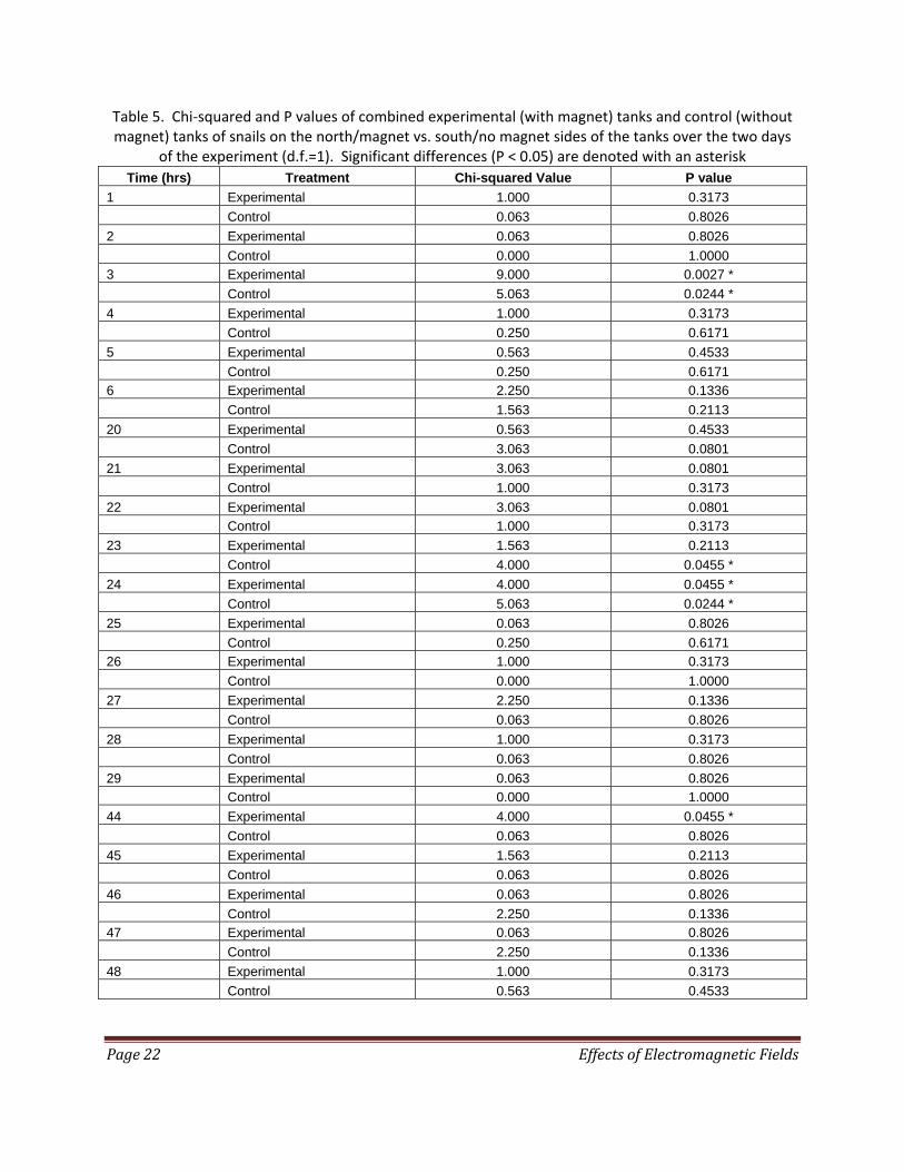
snails in either the control or magnetized tanks (Tables 3 and 4); therefore, we pooled the data for the 4 tanks in each treatment together. Out of 42 possible comparisons of M to U and N to S over the 48‐h study, only 6 showed statistically significant differences at P < 0.05 (Table 5; Figure 6). Of the 6 significantly different comparisons, 1 had fewer snails in the magnetized side M (at t = 3 h), 2 had more snails in the magnetized side M (at t = 24 and 44 h), and 3 control tanks had fewer snails in the N side at t = 3, 23, and 24 h. There was no change in distribution of Elimia that could be attributed to the static magnetic field.

For the Corbicula trials, Fisher’s Exact test did not reveal any significant differences among

individual tanks in the distribution of clams for either the control or magnetized treatments (Tables 6 and 7). Out of 36 possible comparisons of M to U and N to S in the 192‐h study, there were no statistically significant differences in the numbers of clams in the two halves of the tanks, at a probability P < 0.05 (Table 8, Figure 7). The clams did not change their distribution in response to the static magnetic field.

ExperimentswithFreshwaterFish The fathead minnow, Pimephales promelas, is a common stream fish, able to tolerate a wide

range of environmental conditions including high temperatures, low oxygen levels, and high turbidities. They can be found in many of waterways throughout North America east of the Rocky Mountains (Etnier and Starnes 1993). The fish used in these experiments were held in a 0.3m X 0.3m fiberglass tanks with 3‐inch‐long, 3‐inch diameter, opaque PVC half‐cylinders (huts) as cover for each individual for 72 hours prior to the experiment.

As with the snail and clam experiments, permanent magnets were placed under glass aquaria,

and the locations of fathead minnows in magnetized (test) tanks and un‐magnetized (control) tanks were periodically recorded. Three test and three control tanks were used. Both the tanks with magnets and the side of the tank with magnets were selected randomly. There was no sediment on the bottom of the tanks, but the opaque half‐cylinders (huts) were placed in the center of each half of the tank to provide cover for the fish. The male fathead minnows used in these experiments prefer to remain under objects (cover) as part of both normal and breeding behavior. One of the huts was placed directly over the magnet and the other hut was placed on the opposite side of the tank (Figure 8). The fish were free to move from one hut to the other and select a preferred location. Tops of the aquaria were covered and the glass aquaria were placed inside of opaque flumes to minimize disturbance.

Dissolved oxygen concentrations and temperatures were measured in each tank. The

experiments were started in the morning by placing a single fish in each tank without the huts. After the fish had acclimated to the new tanks for fifty‐five minutes, the two huts were placed in each tank. Five minutes later we began recording the locations of the fish, every 5 minutes for 46 hours. Each fish was exposed to the magnetized (test) and control tanks, and the order of treatments was randomized. We were unable to keep track of individual fish, but we did keep the fish exposed to different treatments


Table 3. Probability (P) values from Fisher’s Exact tests done between the individual control tanks of snails at t=6 h (a), 24 h (b), and 48 h (c) after the experiment began

(a)

Tank 1 3 6 8

1 ‐‐ 0.4725 1.0000 0.7224

3 ‐‐ ‐‐ 0.4725 1.0000

6 ‐‐ ‐‐ ‐‐ 0.7224

(b)

Tank 1 3 6 8

1 ‐‐ 0.2852 1.0000 1.0000

3 ‐‐ ‐‐ 0.1489 0.2852

6 ‐‐ ‐‐ ‐‐ 1.0000

(c)

Tank 1 3 6 8

1 ‐‐ 1.0000 0.7224 0.7224

3 ‐‐ ‐‐ 1.0000 1.0000

6 ‐‐ ‐‐ ‐‐ 1.0000

Table 4. Probability (P) values from Fisher’s Exact tests done between the individual test tanks of snails at t=6 h (a), 24 h (b), and 48 h (c)

from the beginning of exposure to a static magnetic field

(a)

Tank 2 4 5 7

2 ‐‐ 1.0000 0.7160 1.0000

4 ‐‐ ‐‐ 0.7160 1.0000

5 ‐‐ ‐‐ ‐‐ 0.7160

(b)

Tank 2 4 5 7

2 ‐‐ 1.0000 0.1489 0.0659

4 ‐‐ ‐‐ 0.2734 0.1351

5 ‐‐ ‐‐ ‐‐ 1.0000

(c)

Tank 2 4 5 7

2 ‐‐ 0.7224 1.0000 1.0000

4 ‐‐ ‐‐ 1.0000 1.0000

5 ‐‐ ‐‐ ‐‐ 1.0000


Table 5. Chi‐squared and P values of combined experimental (with magnet) tanks and control (without magnet) tanks of snails on the north/magnet vs. south/no magnet sides of the tanks over the two days

of the experiment (d.f.=1). Significant differences (P < 0.05) are denoted with an asterisk

Time (hrs) Treatment Chi-squared Value P value

1 Experimental 1.000 0.3173

Control 0.063 0.8026


Control 0.000 1.0000

3 Experimental 9.000 0.0027 *

Control 5.063 0.0244 *


Control 0.250 0.6171


Control 0.250 0.6171


Control 1.563 0.2113


Control 3.063 0.0801


Control 1.000 0.3173


Control 1.000 0.3173


Control 4.000 0.0455 *


Control 5.063 0.0244 *


Control 0.250 0.6171


Control 0.000 1.0000


Control 0.063 0.8026


Control 0.063 0.8026


Control 0.000 1.0000


Control 0.063 0.8026


Control 0.063 0.8026


Control 2.250 0.1336


Control 2.250 0.1336


Control 0.563 0.4533


(a)

0

2

4

6

8

10

12

14

0 7 14 21 28 35 42

Time (hrs)

Nu

mb

er o

f S

nai

ls

mag 2

mag 4

mag 5

mag 7

(b)

0

2

4

6

8

10

12

14

0 7 14 21 28 35 42

Time (hrs)

Nu

mb

er o

f S

nai

ls

L 1

L 3

L 6

L 8

Figure 6. Mean number of snails on the side with the magnet in experimental tanks (a) or the left side of the control tanks (b) over a 48 hour period (n=64, error bars= ±1SE)


Table 6. Probability (P) values from Fisher’s Exact tests done between the individual control tanks of clams at t=16 (a), 48 (b), and 192 (c) hrs

(a)

Tank 3

6 0.6193

(b)

Tank 3

6 1.0000

(c)

Tank 3

6 1.0000

Table 7. Probability (P) values from Fisher’s Exact tests done between the individual test tanks of clams at t=16 (a), 48 (b), and 192 (c) hrs

(a)

Tank 4 5 7

2 1.0000 1.0000 1.0000

4 ‐‐ 1.0000 1.0000

5 ‐‐ ‐‐ 1.0000

(b)

Tank 4 5 7

2 1.0000 1.0000 1.0000

4 ‐‐ 1.0000 1.0000

5 ‐‐ ‐‐ 1.0000

(c)

Tank 4 5 7

2 0.6193 1.0000 1.0000

4 ‐‐ 1.0000 1.0000

5 ‐‐ ‐‐ 1.0000


Table 8. Chi‐squared and probability (P) values of combined test (with magnet) tanks and control (without magnet) tanks of clams on the north/magnet vs.

south/no magnet sides of the tanks over the two days of the experiment (d.f.=1)

Time (hrs) Treatment Chi‐squared P value


Control 0.000 1.0000

20.5 Experimental 0.000 1.0000

Control 0.250 0.6171


Control 0.250 0.6171


Control 0.250 0.6171

44.5 Experimental 0.125 0.7237

Control 0.250 0.6171


Control 0.250 0.6171


Control 0.000 1.0000

116.5 Experimental 0.500 0.4795

Control 0.000 1.0000


Control 0.000 1.0000


Control 0.250 0.6171

140.5 Experimental 0.125 0.7237

Control 0.250 0.6171


Control 0.250 0.6171


Control 0.250 0.6171


Control 0.250 0.6171


Control 0.250 0.6171


Control 0.250 0.6171

188.5 Experimental 0.000 1.0000

Control 0.250 0.6171


Control 0.250 0.6171


(a)

0

1

2

3

4

5

6

0 7

14

21

28

35

42

49

56

63

70

77

84

91

98

105

112

119

126

133

140

147

154

161

168

175

182

189

Time (hrs)

Nu

mb

er o

f C

lam

s

Mag 2

Mag 4

Mag 5

Mag 7

(b)

0

1

2

3

4

5

6

0 7 14 21 28 35 42 49 56 63 70 77 84 91 98 105

112

119

126

133

140

147

154

161

168

175

182

189

Time (hrs)

Nu

mb

er o

f C

lam

s

L 3

L 6

Figure 7. Mean number of clams on the side with the magnet in the experimental tanks (a) or the left side of the control tanks (b) over a 192 hour period (n=16[control], 32 [test], error bars= ±1SE)


Figure 8. Experimental setup for the fathead minnow studies. The black rectangles representing the placement of the magnets relative to the grids

on the bottom of the tanks and the grey horseshoes represent the huts (cover structures for fish)


separate from each other to ensure each fish experienced each treatment. The fish were not fed during the 46‐hour experiments, but were fed Tetramin fish flakes before and between experiments.

Video cameras were set up between the tanks (Figure 8). Using an Image Vault® security

system, we recorded the locations of the fish directly from the video images every five minutes between 0620 and 1820 hours, when the room was illuminated by overhead lights. The video images from each test and control tank were examined to determine if the fish were (1) in the hut on the north, (2) out of the hut on the north, (3) in the hut on the south, or (4) out of the hut on the south sides of the test and control tanks.

Results

Throughout the experiments, fathead minnows were observed in every location within the tanks, that is, on both magnetized and un‐magnetized (or North and South sides) as well as both inside and outside of the huts. The fish changed locations frequently in both the test and control tanks (Figure 9).

Figure 9. Activity of fathead minnows in un‐magnetized control tanks and magnetized treatment tanks.

Each line represents an individual fish, and depicts the number of times that fish was found at the opposite side of the tank from the previous observation


Fathead minnows in the test tanks (with magnets) spent large amounts of time both inside and outside of the huts (Table 9; Figure 10). Out of 272 observations in each experiment and tank combination, fish were found inside the huts on an average of 151 times (56%) for control tanks and 144 times (53%) for test tanks. There was no indication that the presence of the static magnetic field caused the fathead minnows to either seek or avoid shelter in the huts.

The fathead minnows were observed on both the magnetized and un‐magnetized sides of the

test tanks. Out of 272 observations in each experiment and tank, the fish were recorded on the magnetized side of the test tanks an average of 138 times (51%; Table 9). Chi‐square testes with Yates correction were performed on individual experiment/tank combinations to determine whether locations were significantly different from a uniform distribution, i.e., 136 (50%) of the observations on each side. In some experiment/tank combinations, minnows were recorded at significantly higher percentages on the magnetized side of the tanks (P < 0.05; 3 out of 12 comparisons). On the other hand, in 4 out of 12 comparisons, significantly higher percentages of minnows were found on the un‐magnetized side. Five of the 12 comparisons, and the overall total for the 12 experiment/tank combinations, did not show statistically significant differences in location over the course of the 46‐hour experiments (Table 9). Owing the frequent movements, lack of a consistent preference for magnetized or un‐magnetized sides, and an overall uniform distribution of fish, there was no indication that fathead minnows were either attracted to or repelled by the static magnetic fields in these tests.



Table 9. Locations of individual fathead minnows during static magnetic field exposure experiments. Values are the number of observations (made at 5‐minute intervals) of fish locations during the 46‐hour‐long experiment. Control tanks were divided into North (N) and South (S) sides. Test tanks were divided into magnetized (M) and un‐magnetized (U) sides. P values are the probabilities that the minnows preferred one side of

the tank over the other side, based on Chi square tests with Yates’ correction Experiment

number Control tanks (without magnets) Test tanks (with magnets)

Tank number

Inside hut N

Outside hut N

Inside hut S

Outside hut S

P value (N vs. S)

Tank number

Inside hut M

Outside hut M

Inside hut U

Outside hut U

P value (M vs. U)

1

1 198 31 15 28 <0.01 2 147 52 35 38 <0.01 3 166 45 34 27 <0.01 5 87 9 168 8 <0.01 6 21 103 24 124 0.34 7 260 4 8 0 <0.01

2

1 116 67 17 72 <0.01 2 204 12 47 9 <0.01 3 81 12 161 18 <0.01 5 93 25 118 35 0.16 6 13 112 1 146 0.39 7 39 78 47 108 0.12

3

2 186 2 58 26 <0.01 1 51 62 16 143 0.06 5 77 52 88 55 0.61 3 36 69 28 139 <0.01 7 96 42 44 90 0.93 6 38 78 51 105 0.10

4

2 195 18 48 11 <0.01 1 21 29 126 96 <0.01 5 9 136 8 119 0.49 3 27 81 69 95 0.02 7 89 58 62 63 0.39 6 0 149 7 116 0.30

Total number of observations

1247 678 560 779 <0.01 1003 648 720 892 0.65

Average number of observations

104 57 47 65 84 54 60 74



Experiment 1 (August 2-4, 2010)




Figure 10. Percent of time that fathead minnows spent inside and outside of the huts on the

magnetized sides (M) and un‐magnetized sides (U) of the test tanks. Numbers in blocks represent number of observations (out of a total of 272) during each 46‐hour experiment



5. SummaryandRecommendations

Experiments to date have shown no evidence that 3 common freshwater taxa (snail, clam, and fish species) were either attracted to or repelled by the static magnetic field created by the permanent bar magnet. In future experiments we will (1) increase the strength of the static magnetic field, (2) test other freshwater fish and macroinvertebrate species, and (3) examine other behavioral responses in fish (e.g., C‐start reactions) that are relevant to identifying possible effects of EMF associated with HK projects in rivers. We will carry out EMF experiments using a variable magnetic field, similar to one which would be created by the MHK generator or the transmission of alternating current (AC) along the underwater electrical cable. As the MHK industry develops to the point that prototype devices are tested in rivers, we plan to make field measurements of these prototypes to verify that the static and variable magnetic fields tested in our experiments are representative.



6. References

Basov, B.M. 1999. Behavior of sterlet Acipenser ruthenus and Russian sturgeon A. gueldenstaedtii in

low‐frequency electric fields. Journal of Ichthyology 39(9):782‐787.

Basov, B.M. 2007. On electric fields of power lines and on their perception by freshwater fish. Journal

of Ichthyology 47(8):656‐661.

Boles, L.C. and K.J. Lohmann. 2003. True navigation and magnetic maps in spiny lobsters. Nature

421:60‐63.

Bochert R. and M.I. Zettler. 2006. Effect of electromagnetic fields on marine organisms. Chapter 14 in:

Offshore Wind Energy. J. Koller, J. Koppel, and W. Peters (eds.). Springer‐Verlag, Berlin.

CMACS (Centre for Marine and Coastal Studies). 2003. A Baseline Assessment of Electromagnetic Fields

Generated by Offshore Windfarm Cables. COWRIE Report EMF‐01‐2002 66. Liverpool, UK.

http://www.offshorewind.co.uk (accessed August 20, 2008).

Collin, S.P. and D. Whitehead. 2004. The functional roles of passive electroreception in non‐electric

fishes. Animal Biology 54(1):1‐25.

DOE (U.S. Department of Energy). 2009. Report to Congress on the Potential Environmental Effects of

Marine and Hydrokinetic Energy Technologies. December 2009. 89 p. + appendices.

http://www1.eere.energy.gov/windandhydro/marine_hydro_market_acceleration.html

DON (U.S. Department of the Navy). 2003. Environmental Assessment – Proposed Wave Energy

Technology Project. Marine Corps Base Hawaii, Kaneohe Bay, Hawaii. Office of Naval Research.

Etnier, D. A. and W. C. Starnes (1993). The Fishes of Tennessee. University of Tennessee Press: Knoxville,

TN, p. 250‐252.

Gill, A.B., I. Gloyne‐Phillips, K.J. Neal, and J.A. Kimber. 2005. The Potential Effects of Electromagnetic

Fields Generated by Sub‐Sea Power Cables Associated with Offshore Wind Farm Developments on

Electrically and Magnetically Sensitive Marine Organisms – A Review. COWRIE Report EM Field 2‐06‐

2004. http://www.offshorewind.co.uk (accessed May 1, 2008).

Kalmijn, A.T. 2000. Detection and processing of electromagnetic and near‐field acoustic signals in

elasmobranch fishes. Philosophical Transactions of the Royal Society of London B. 355:1135‐1141.

Lohmann, K.J. and C.M.F. Lohmann 1996. Detection of magnetic field intensity by sea turtles. Nature

380:59‐61.


Ohman, M.C., P. Sigray, and H. Westerberg. 2007. Offshore windmills and the effects of electromagnetic

fields on fish. Ambio 36(8):630‐633.

Skauli, K.S., J.B. Reitan, and B.T. Walther. 2000. Hatching in zebrafish (Danio rerio) embryos exposed to

a 50Hz magnetic field. Bioelectromagnetics 21:407‐410.

Walker, M.M., C.E. Diebel, C.V. Haugh, P.M. Pankhurst, J.C. Montgomery, and C.R. Green. 1997.

Structure and function of the vertebrate magnetic sense. Nature 390:371‐376.

Wilkens, L.A. and M.H. Hoffman. 2005. Behavior of animals with passive, low‐frequency electrosensory

systems. Pages 229‐263 In: Electroreception. T.H. Bullock, C.D. Hopkins, A.N. Popper, and R.R. Fay

(eds.). Springer Handbook of Auditory Research Volume 21, Springer, New York.

Woytenek, W., X. Pei, and L.A. Wilkens. 2001. Paddlefish strike at artificial dipoles simulating the weak

electric fields of planktonic prey. The Journal of Experimental Biology 204:1391‐1399.

APPENDIX A.

EMF QUESTIONNAIRE TO MHK DEVELOPERS AND RESEARCH INSTITUTIONS

A-1

Appendix A.

EMF Questionnaire to MHK Developers and Research Institutions

Dear Sir:

With the support of the U.S. Department of Energy’s Water Power Program, scientists at Oak Ridge National Laboratory and Pacific Northwest National Laboratory will soon begin studies of the effects of marine and hydrokinetic (MHK) energy technologies on aquatic animals. We are asking your assistance in the development of a study of the potential biological effects of electromagnetic fields (EMF). The EMF could arise from the MHK devices themselves or from individual cables, networks of cables, and transformers used to transmit electricity to shore. It is known that some aquatic organisms are sensitive to electric fields (e.g., sharks, eels, freshwater paddlefish, and sturgeons) and magnetic fields (e.g. eels, lobsters, trout, salmon, and sea turtles). However, to our knowledge the EMFs associated with new MHK designs have not been quantified, and there are significant gaps in knowledge regarding sources and biological effects of EMF in the aquatic environment.

In order to recreate representative electrical and magnetic fields in laboratory experiments, we need to determine the levels of EMF to which aquatic biota will be exposed by MHK projects. Ideally, this would come from in situ measurements of the device and its transmission cables. Alternatively, we can estimate the EMF based on information about the type of electrical transmission cable to be employed and the nature of the electrical current passing through it.

Your answers to the following questions would be very useful to our experimental design.

1. What measurements of the electrical and magnetic fields from your MHK project have been made?

2. What type of electrical transmission cable(s) will be used for your project? For example:

a. the number of wires in a cable, b. cable diameter, c. composition of the internal core conductor cables, d. composition of the overall cable(s), e. Reference to a particular design, manufacturer, and model number would be helpful.

3. Describe the electrical current that will be transmitted

a. AC or DC b. amperage c. voltage d. power

Any documents or references that you can provide would be greatly appreciated. Thank you very much for your assistance.

A‐2

ORNL/TM‐2011/244

INTERNAL DISTRIBUTION

1. M. S. Bevelhimer 6. J. W. Saulsbury 2. G. F. Cada 7. P. E. Schweizer 3. G. K. Jacobs 8. G. P. Zimmerman 4. L. Liang 9. ORNL Office of Technical Information 5. M. J. Peterson and Classification

EXTERNAL DISTRIBUTION

10. Kristina P. Riemer, Lawrence University, SPC Mailbox 1227, 711 East Boldt Way, Appleton, WI 54911

11. Jocelyn Brown‐Saracino, U.S. Department of Energy, Office of Wind and Hydropower Technology Program, Forrestal Building, EE‐2B, 1000 Independence Avenue, S.W., Washington, DC 20585

12. Julie W. Turner, Grinnell College, Department of Biology, 1116 Eight Avenue, Grinnell, IA 50112

Documents

Effects on Freshwater Organisms of Magnetic Fields ... · of Magnetic Fields Associated with Hydrokinetic Turbines ... EFFECTS ON FRESHWATER ORGANISMS OF MAGNETIC FIELDS ... The electric