Department of Environmental Science

Master in Environmental Science

Major in Ecology and Evolution

Effects of tributaries on mainstem periphyton assemblages in relation to

catchment landuse

Master thesis

Fulfillment of the requirements for the Master of Science ETH in Environmental Science

(Msc ETH Environmental Sc.)

Submitted by:

Michael Scheurer

Supervisors:

1st Dr. Christopher Robinson, EAWAG

2nd Dr. Christian Stamm, EAWAG

August 2010

2

Contents

1 Introduction ..................................................................................................................................... 4

2 Materials and Methods ................................................................................................................... 5

2.1 Study area ................................................................................................................................ 5

2.2 Study sites................................................................................................................................ 5

2.3 Sampling .................................................................................................................................. 7

2.4 Laboratory analysis .................................................................................................................. 8

2.5 Statistics................................................................................................................................... 9

3 Results ........................................................................................................................................... 10

3.1 Physical characterization ....................................................................................................... 10

3.2 Chemical characterization ..................................................................................................... 12

3.3 Periphyton assemblages ........................................................................................................ 15

4 Discussion ...................................................................................................................................... 19

5 Conclusion ..................................................................................................................................... 21

6 References ..................................................................................................................................... 22

6.1 Internet links ......................................................................................................................... 22

6.2 Figure references ................................................................................................................... 23

Abbreviations

ANOVA: Analysis of variance NTU: Nephelometric turbidity unit

AFDM: Ash free dry mass PN: Particulate nitrogen

AI: Autotrophic index POC: Particulate organic carbon

DN: Dissolved nitrogen PP: Particulate phosphorus

DOC: Dissolved organic carbon RCC: River continuum concept

DP: Dissolved phosphorus SDC: Serial discontinuity concept

GIS: Geographic information system TIC: Total inorganic carbon

3

Abstract

The spatial importance of tributaries along a river has been shown in several studies. Tributa-

ries reflect the anthropogenic activities within the catchment and, due to their interruption of

the river continuum, they form heterogeneous in which biodiversity and productivity may be

enhanced. If productivity rises, we also should find changes in primary production and periphy-

ton community structure. The ecological importance of periphyton has been a topic of numer-

ous studies. Based on these two aspects, I hypothesized that periphyton community structure

differs between tributaries draining different kinds of land use types regarding biomass, chlo-

rophyll-a and taxa composition. I also expected tributaries to affect mainstem periphyton

community structure as reflected in the basic land use in the respective catchment.

To test these predictions, I analysed in winter 2009-2010 nine confluence zones comprising

tributaries draining three different land use types: urban, agricultural and natural. Six conflu-

ence zones were within the Mönchaltdorfer-Aa catchment and three within the Kempt catch-

ment. Both catchments are located near Zurich and can be defined as pre-alpine river systems.

After defining three sub-sites per confluence zone (upstream, downstream and tributary), vari-

ous samples were collected and a rough physical characterisation of each site was performed. I

took water samples for chemical analysis and replicate stones (n = 10) with periphyton for ana-

lysing ash free dry mass (AFDM), chlorophyll-a and taxa composition of the algae. The results

did not support the two hypotheses. I therefore suggest that the outcome of the study would

have differed if the survey was carried out during spring/summer when the effects of land use

on streams are likely most pronounced.

4

1 Introduction

The longitudinal characteristics of a river system including discharge, substrate size and other

physical parameters, and the ecological development along its continuum are generally based

on the river continuum concept (RCC) (Vannote et al. 1980). Nevertheless, the RCC, being a cli-

nal concept, does not look at habitat discontinuities as being physically and biologically impor-

tant. The confluence zones of tributaries with the mainstem are physical disturbances in the

river continuum. Rice et al. (2001) showed that species richness of invertebrates are highest in

confluence zones and can thus be regarded as biological hotspots. It was speculated that the

reason for this peak in biodiversity was a higher habitat complexity and productivity. These

hotspots are distributed discontinuously along a river and could rather be described in line with

the serial discontinuity concept (SDC) instead of the RCC (Ward 1983; Stannford 1995). The SDC

focuses on the interruption of resource continua. These interruptions are, for example, an

abrupt change in water volume, nutrient concentration or general water quality, exactly the

factors in which a tributary may be able to influence the main stream (Rice et al. 2001). Here we

must take into account that these effects vary between different kinds of catchments regard-

ing their basic land use (Hynes 1975; Likens et al. 1977). A tributary draining an agricultural area

can have higher nutrient, salt or even herbicide or pesticide concentrations than a tributary

flowing through a natural catchment. Even though the importance tributaries are often dis-

cussed and their high abundance in river networks, the empirical analysis of tributary effects on

mainstems are quite rare.

Regarding the ecological effects of tributaries on mainstems, we must also include the influ-

ence on periphyton communities. Attached to submerged surfaces, periphyton communities

are composed of photoautotrophic algae, bacteria, protozoa, fungi and detritus, all having vari-

ous key roles in aquatic ecosystems. They can affect water chemistry, habitat availability and

food web dynamics (Larned 2010). In many cases, periphyton is, next to fallen leaves from ripar-

ian vegetation, the primary source of energy for a river system and provides habitat and food

resources for invertebrates and fish. Therefore, periphyton increases the overall productivity of

river ecosystems (Azim 2005). Besides being an energy source, Vymazal (1987) showed that pe-

riphyton has an enormous purification potential by taking up and retaining nitrogen and phos-

phorus. An additional function of periphyton is as an indicator of water quality. Due to the

naturally high number of species and the sensitivity / tolerance of some taxa to changes in

nutrient availability and chemical conditions, the periphyton composition reflects the water

quality and general health of the river ecosystem (Vis 1997).

5

These attributes of periphyton assemblages lead to two major hypotheses that were tested in

the present study.. First, periphyton community structure varies between different kinds of

land us types in terms of biomass, chlorophyll-a and taxa composition. Second, tributaries dif-

ferently affect periphyton assemblages in mainstem rivers depending on the dominant land

use in the tributary catchment.

2 Materials and Methods

2.1 Study area

For the study, two river systems were chosen. One was the Mönchaltdorfer-Aa, a main inflow

into Lake Greifensee. The Aa was selected as a study system for the NRP61 project iWaQa (Link

1, see references), thus the data collected in my study could be used directly within the iWaQa

project (Link 2, see references). The second river was the Kempt, a stream near Dübendorf. Due

to its similar size and land use in its catchment, the Kempt served well as a second study

catchment. Both systems can be characterized as pre-alpine rivers.

2.2 Study sites

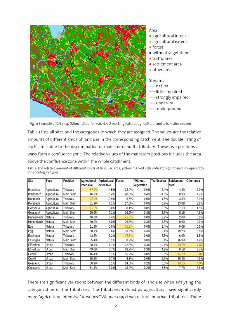
The sampling sites were chosen based on GIS (Geographic Information System) maps (Fig. 2).

The layers for basic land use and stream geomorphology provided the necessary information

to define the sampling sites. The tributaries were categorized depending on the dominant

land use type within the watershed, such as urban (settlement area), agricultural (intensive,

extensive) and natural (forest). Six sites in the Mönchaltdorfer-Aa system and three sites at

the Kempt were selected based on these categories. In total, three urban, three agricultural

and three natural tributaries were chosen (two of each category within the Mönchaltdorfer-

Aa and one within the Kempt system).

Fig. 1 Map of Switzerland, red circle marking the study systems delineated with a black line.

6

Table 1 lists all sites and the categories to which they are assigned. The values are the relative

amounts of different kinds of land use in the corresponding catchment. The double listing of

each site is due to the discrimination of mainstem and its tributary. These two positions al-

ways form a confluence zone. The relative values of the mainstem positions includes the area

above the confluence zone within the whole catchment.

Tab. 1: The relative amount of different kinds of land use area, yellow marked cells indicate significance compared to other category types.

Site Type Position Agricultural

intensive

Agricultural

extensive

Forest Without

vegetation

Traffic area Settlement

area

Other area

Brandbach Agricultural Tributary 57.9% 4.5% 28.9% 0.0% 2.4% 4.3% 2.0%

Brandbach Agricultural Main Stem 46.9% 6.4% 28.0% 0.4% 4.8% 8.9% 4.7%

Rohrbach Agricultural Tributary 70.4% 10.9% 6.6% 0.0% 4.5% 4.5% 3.1%

Rohrbach Agricultural Main Stem 51.9% 7.1% 17.5% 0.0% 6.7% 13.0% 3.8%

Gossau A Agricultural Tributary 65.3% 8.0% 8.1% 0.0% 9.5% 7.1% 1.9%

Gossau A Agricultural Main Stem 59.6% 7.1% 16.5% 0.3% 3.7% 8.1% 4.6%

Hühnerbach Natural Tributary 46.3% 3.4% 43.5% 0.0% 3.9% 2.0% 0.8%

Hühnerbach Natural Main Stem 49.0% 6.0% 26.5% 0.3% 4.8% 9.0% 4.3%

Egg Natural Tributary 61.5% 0.0% 36.6% 0.0% 1.4% 0.0% 0.5%

Egg Natural Main Stem 30.1% 10.6% 33.2% 0.3% 3.1% 19.2% 3.5%

Esslingen Natural Tributary 43.6% 3.2% 42.3% 0.0% 3.5% 6.0% 1.5%

Esslingen Natural Main Stem 55.4% 8.1% 8.9% 0.0% 6.4% 16.9% 4.2%

Effretikon Urban Tributary 38.1% 1.1% 22.5% 0.3% 9.6% 20.6% 7.8%Effretikon Urban Main Stem 49.0% 5.7% 28.3% 0.3% 4.9% 8.1% 3.7%

Oetwil Urban Tributary 46.4% 8.1% 16.7% 0.0% 9.5% 16.3% 3.0%Oetwil Urban Main Stem 50.5% 9.7% 8.8% 0.0% 5.6% 20.4% 4.9%

Gossau U Urban Tributary 50.9% 5.1% 14.0% 0.2% 6.3% 18.5% 4.9%Gossau U Urban Main Stem 61.4% 7.3% 13.9% 0.2% 5.5% 7.7% 3.8%

There are significant variations between the different kinds of land use when analyzing the

categorization of the tributaries. The tributaries defined as agricultural have significantly

more "agricultural intensive" area (ANOVA, p=0.049) than natural or urban tributaries. There

Area

● agricultural intens.

● agricultural extens.

● forest

● without vegetation

● traffic area

● settlement area

● other area

Streams

── natural

── little impaired

── strongly impaired

── unnatural

─ ─ underground

Fig. 2: Example of GIS map (Mönchaltdorfer-Aa), N,A,U marking natural, agricultural and urban sites chosen

7

is no significant difference (ANOVA, p=0.142) when comparing the extensive agricultural area

between tributary categories, but the extensive area has very low values compared to the

intensive and can therefore be neglected. Looking at the amount of forest in the tributary

catchments, we see a significantly higher value for the natural category (ANOVA, p=0.013).

The area without vegetation can also be neglected due to its very low abundance. The

amount of traffic area shows no significances between the different kinds of tributaries

(ANOVA, p=0.092), but a trend of higher values in urban areas is visible. Looking at the set-

tlement area, there is a highly significant difference of urban tributaries from the other cate-

gories (ANOVA, p=0.0003). The last column "other area" can be neglected as well, although

there is significantly more "other area" within the urban tributary catchments (ANOVA,

p=0.032). These GIS-based data perfectly supports the categorisation of the chosen tributar-

ies.

As can be seen in the site table, there is a double listing for Gossau. This is due to the very

close situation of two different sites, one agricultural and one urban. To prevent misunder-

standings regarding site names, Gossau will always be followed by a U for urban and A for

agricultural.

2.3 Sampling

Sampling started on 28 January 2010 with the site called Egg. By 18 February 2010, all six sites in

the Mönchaltdorfer-Aa system were sampled. The three other sites in the Kempt system were

sampled between 25 February and 3 March 2010. Sampling could only be done once, otherwise

the generated amount of data could not have been processed within the six month time limit

of the master thesis. It must be noted that each site was sampled during one day, so there is no

difference in date for any one site.

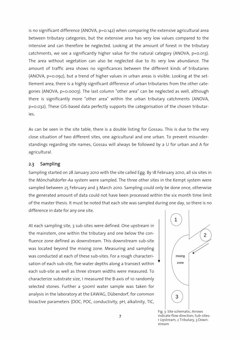
At each sampling site, 3 sub-sites were defined. One upstream in

the mainstem, one within the tributary and one below the con-

fluence zone defined as downstream. This downstream sub-site

was located beyond the mixing zone. Measuring and sampling

was conducted at each of these sub-sites. For a rough characteri-

sation of each sub-site, five water depths along a transect within

each sub-site as well as three stream widths were measured. To

characterize substrate size, I measured the B-axis of 10 randomly

selected stones. Further a 500ml water sample was taken for

analysis in the laboratory at the EAWAG, Dübendorf, for common

bioactive parameters (DOC, POC, conductivity, pH, alkalinity, TIC,

1

2

3

mixing

zone

Fig. 3: Site schematic; Arrows indicate flow direction; Sub-sites: 1 Upstream, 2 Tributary, 3 Down-stream

8

NH4-N, NO2-N, NO3-N, DN, PN, PO4-P, DP, PP). Temperature, conductivity and pH were also

measured on the field with a combo pH & EC device (Hanna, Combo pH & EC). Turbidity meas-

urements were taken twice at each sub-site with an optical turbidity meter (Cosmos, Züllig AG).

To make any conclusions regarding tributary effects, I quantified the discharge ratio of tribu-

tary / main stem. At each sub-site, discharge measurements were conducted using a Doppler

velocity meter (Flow tracker, SonTek). For an accurate discharge measurement, it was crucial to

pick a transect with a consistent depth and doing as many measurements within a transect as

possible. All velocity readings were taken at 60% depth and the discharge was automatically

calculated by the device.

Finally, 10 stones with periphyton cover were collected per sub-site. This collection of stones

was not completely random, but represented the different kinds of periphyton patches within

each sub-site. These stones were put into a zip-lock bag, returned to the lab in a cooler, and

stored in a freezer at -20°C for further analysis.

2.4 Laboratory analysis

For each of the 10 stones per sub-site, three parameters were analysed, including ash free dry

mass, chlorophyll-a and taxa composition. First, the stones were left to thaw within the zip-lock

storage bag. From each stone, an area of 9cm2 was scraped of periphyton and placed in an Er-

lenmeyer flask with a total amount of 100ml water. The scraping was conducted with a dremel

(Model 395) and a steel brush (dremel ID:442) at the lowest speed level ( 10'000 rpm).

Fig. 4: Stone with scraped area, right top corner of dish: Plexiglas template used for scraping

9

Two filtrations of this 100ml solution were carried out. For chlorophyll-a analysis, 10ml of this

periphyton solution were filtered (Whatman, GF/F, Ø 47mm), and the filter was put into a glass

tube filled with 8ml of 90% ethanol. To assure a proper extraction of the chlorophyll, all tubes

were put into a hot water bath at 60°C for 10 minutes. After extraction, the samples were cov-

ered with aluminium foil and stored at 4°C until analyzed with the HPLC. In a second step, the

ash free dry mass was analyzed. Here, 25ml of the basic solution was filtered and the filters

placed in a ceramic dish for drying. After drying (Binder, FD 115) for at least two days at 60°C, the

samples were weighed, burned at 500°C for four hours (Oven: Nabertherm, Model N150) and

then weighed again. The weight difference before and after burning corresponds to the ash

free dry mass.

From these two parameters, AFDM and chlorophyll-a concentration, the autotrophic index (AI)

was generated. By simply dividing AFDM/chlorophyll-a concentrations, the value tells us how

strong a system is affected by organic pollutants. According to Collins & Weber (1978), AI values

between 50 and 100 indicate non-polluted systems and autotrophs are dominating the system.

Values between 100 and 400 define a system affected by organic substances. Systems with

values higher than 400 are dominated by heterotrophs and have high concentrations of or-

ganic pollutants.

For a semi-quantitative (categories: 1 sporadic, 2 seldom, 3 regularly, 4 frequent, 5 dominant)

taxonomic analysis of the collected periphyton assemblages, a 3ml algae solution from each

stone per sub-site was placed in a storage vial and later analysed by an Eawag technician.

2.5 Statistics

The statistical analysis was carried out with two statistic programs. Analysis of variance

(ANOVA) and plotting of regressions was done with JMP (SAS) and principal component analy-

sis (PCA) was made using Statistica (StatSoft).

Analysing the variation of data within stream types and position and between sites was con-

ducted by a one factorial ANOVA. This test was used to indentify significant differences among

the data.

To compare the results of AFDM, chlorophyll-a and autotrophic index between stream types

and positions a Tukey-test was performed.

The high amount of variables from the chemical analysis, was reduced to a manageable

amount of principal components by carrying out a PCA.

10

To be able to see any relations between species richness, chlorophyll-a, AFDM and the AI a cor-

relation matrix was generated.

3 Results

3.1 Physical characterization

The physical parameters give a rough impression of the study streams. As seen in figure 5, the

mean width range ranges from about 1 meter at the tributary site at Egg to nearly 8 meters at

the Brandbach downstream site. Comparing all sites (downstream sub-sites excluded), the

tributaries are, as expected, significantly smaller (p=0.024) than the main stem. Mean depths

(Fig. 6) ranged from 6 cms at the tributary site at Egg to nearly 40 cm at the Effretikon main

stem site, and there is no significant difference between the tributaries and the main stem

(p=0.138).

The 10 randomly measured stones at each sub-site resulted in mean values ranging from 3.5 cm

at the Esslingen tributary site to 11.6 cm at the Gossau A upstream sub-site. No significance

difference between tributaries and respective mainstems (p=0.594) or between land use types

(p= 0.834) could be detected.

The turbidity measured at all sites was in

general quite similar (Fig. 7). At the Brand-

bach (agricultural), the mainstem sub-sites at

Egg (natural), the tributary sub-site at Gossau

(agricultural) and the Oetwil (urban) site had

the highest NTU values. Here it must be

noted that the maximum depth was so low at

some sites that it could have affected the

accuracy of the turbidity meter, although this

Fig. 5: Mean width of each sub-site Fig. 6: Mean depth of each sub-site

Fig. 7: Mean NTU values of each sub-site

11

is not the case at each site with high NTU values.

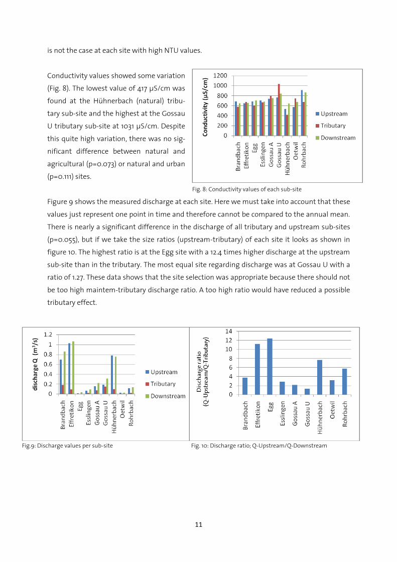
Conductivity values showed some variation

(Fig. 8). The lowest value of 417 µS/cm was

found at the Hühnerbach (natural) tribu-

tary sub-site and the highest at the Gossau

U tributary sub-site at 1031 µS/cm. Despite

this quite high variation, there was no sig-

nificant difference between natural and

agricultural (p=0.073) or natural and urban

(p=0.111) sites.

Figure 9 shows the measured discharge at each site. Here we must take into account that these

values just represent one point in time and therefore cannot be compared to the annual mean.

There is nearly a significant difference in the discharge of all tributary and upstream sub-sites

(p=0.055), but if we take the size ratios (upstream-tributary) of each site it looks as shown in

figure 10. The highest ratio is at the Egg site with a 12.4 times higher discharge at the upstream

sub-site than in the tributary. The most equal site regarding discharge was at Gossau U with a

ratio of 1.27. These data shows that the site selection was appropriate because there should not

be too high maintem-tributary discharge ratio. A too high ratio would have reduced a possible

tributary effect.

Fig.9: Discharge values per sub-site Fig. 10: Discharge ratio; Q-Upstream/Q-Downstream

Fig. 8: Conductivity values of each sub-site

12

Date

Site

TypeP

ositionD

OC

PO

CC

onductivitypH

Alkalinity

TICN

H4 -N

NO

2 -N N

O3 -N

DN

PN

PO

4-PD

PP

P

mg C

/Lm

g C/L

µS/cm

mm

ol/Lm

g C/L

µg N/L

µg N/L

mg N

/Lm

g N/L

mg N

/Lµg P

/Lµg P

/Lmg P

/L

28.01.2010E

gg N

aturalD

ownstream

3.11.94

6388.15

5.6467.7

1232.017.6

2.03.9

0.21192.4

201.410.9

28.01.2010E

gg N

aturalTributary

1.60.30

5508.12

6.0372.4

26.91.2

1.92.0

0.0310.8

13.92.2

28.01.2010E

gg N

aturalU

pstream2.9

1.96619

8.205.50

66.01015.0

11.81.9

3.00.20

138.6156.6

11.2

28.01.2010R

ohrbachA

griculturalD

ownstream

3.71.33

8597.93

5.2362.8

984.0147.2

9.110.4

0.1913.4

27.515.6

28.01.2010R

ohrbachA

griculturalTributary

2.30.45

6108.19

6.2274.6

15.64.6

3.13.3

0.0310.5

14.62.7

28.01.2010R

ohrbachA

griculturalU

pstream3.2

1.19824

7.895.24

62.976.4

117.88.9

9.10.16

11.423.4

11.2

04.02.2010G

ossau UU

rbanD

ownstream

2.80.71

7588.01

6.0172.1

18322.5

3.63.6

0.076.1

9.9<1.0

04.02.2010G

ossau UU

rbanTributary

3.81.14

9597.68

4.6455.7

1774179.0

9.311.2

0.157.4

19.46.2

04.02.2010G

ossau UU

rbanU

pstream2.6

0.58717

8.096.09

73.025.1

6.12.8

2.90.06

5.08.4

1.1

04.02.2010G

ossau AA

griculturalD

ownstream

2.70.70

6868.11

5.9070.8

9.94.6

2.72.8

0.066.9

10.8<1.0

04.02.2010G

ossau AA

griculturalTributary

2.10.50

7448.05

5.7569.0

7.15.6

3.73.8

0.056.0

9.0<1.0

04.02.2010G

ossau AA

griculturalU

pstream2.7

0.77689

8.085.88

70.57.4

4.12.3

2.40.06

5.98.8

<1.0

11.02.2010E

sslingenN

aturalD

ownstream

2.30.40

6548.27

6.1874.2

8.93.0

2.93.0

0.0428.1

28.7<1.0

11.02.2010E

sslingenN

aturalTributary

1.80.30

6168.22

6.2474.9

<5.01.3

2.12.2

0.0229.7

30.4<1.0

11.02.2010E

sslingenN

aturalU

pstream2.7

0.42656

8.236.24

74.97.5

3.62.9

3.10.04

27.428.3

<1.0

18.02.2010O

etwil

Urban

Dow

nstream2.4

1.49538

8.255.35

64.223.3

6.22.3

2.30.13

23.226.5

3.8

18.02.2010O

etwil

Urban

Tributary2.2

0.48631

8.416.02

72.27.2

4.71.9

1.80.06

109.5116.6

2.6

18.02.2010O

etwil

Urban

Upstream

2.10.73

4667.94

4.4953.8

121.712.2

2.52.4

0.075.2

7.32.5

25.02.2010B

randbachA

griculturalD

ownstream

2.50.94

5957.82

5.4965.9

21.19.9

3.93.9

0.1014.4

18.216.8

25.02.2010B

randbachA

griculturalTributary

2.10.85

5288.06

5.6667.9

10.41.5

5.05.0

0.063.0

22.47.7

25.02.2010B

randbachA

griculturalU

pstream2.2

0.97625

7.845.50

66.080.3

39.54.2

4.20.11

17.925.4

17.8

03.03.2010E

ffretikonU

rbanD

ownstream

1.90.53

5857.98

6.0973.0

< 17.8

4.44.4

0.0416.4

23.24.1

03.03.2010E

ffretikonU

rbanTributary

2.10.63

5988.01

6.2274.6

< 15.2

4.64.7

0.045.8

18.93.1

03.03.2010E

ffretikonU

rbanU

pstream2.1

0.56582

8.156.03

72.41.2

5.94.2

4.30.04

17.920.4

3.2

03.03.2010H

ühnerbachN

aturalD

ownstream

2.50.50

5877.99

5.9971.9

34.827.4

4.74.7

0.0518.9

27.55.7

03.03.2010H

ühnerbachN

aturalTributary

1.50.45

4778.05

5.4565.4

< 11.9

3.93.9

0.036.2

8.02.6

03.03.2010H

ühnerbachN

aturalU

pstream2.1

0.91605

7.956.11

73.338.0

31.84.7

4.80.06

18.822.5

5.0

3.2 Chemical characterization

Chemical analysis of the water samples taken at each sub-site was conducted by the AuA-

Laboratory at Eawag, Dübendorf. Table 2 shows all the results of the analysis.

Tab. 2: Summary table of chemical analysis for each sub site.

13

Regarding all sub-sites (up-, downstream, tributary) as one, chemical analysis of the two river

systems showed no significant differences between the different kinds of land use categories.

Even by solely analyzing tributaries or main stem (up-, donwstream) in land use categories, no

significant difference in chemical components was visible. However, some sites showed ele-

vated values for some specific parameters. For example Gossau U had a very high mean con-

ductivity value of 811.3 µS/cm and the variation among all sites showed a significant difference

(p=0.003). Another outlier site was Rohrbach with a mean NO3-N concentration of 7.02 mg/L.

The overall variation between sites for NO3-N was also significant (p=0.032). It must be noted

that this high mean value was derived from the mainstem sub-sites (up-, downstream) having

a mean concentration of 9.0 mg/L. The tributary at 3.6 mg/L was close to the overall mean of

3.9 mg/L. For the PO4-P and DP components, the Egg site had extremely high mean values of

PO4-P (113.9 µg/L) and DP (123 µg/L). Here we have the same situation as for NO3-N in which the

very high mean values were derived from the mainstem sub-sites.

A multivariate statistical analysis was done using principal component analysis. This reduces

the high amount of variables to a manageable number of principal components. Before per-

forming a PCA with Statistica all the data was log(x+1) transformed. The PCA analysis was car-

ried out with the most biological relevant parameters such as DOC, POC, conductivity, pH, NO3-

N, PN, PO4-P, PP, and turbidity. The first principal component (PC1) shows that DOC, POC, PN

and PP have a higher (or lower) loading value than +(-)0.7 and explain 44% of the total variation

among sites. NO3-N and PO4-P had a higher loading value than +(-)0.7 for PC2, and explain 25%

of the total variation among sites. The first two principal components together explained 69%

of the total variation among sites.

14

Figure 11 shows the PCA scores of all sites separately. Here you can see how the tributary

ences the respective mainstem. At sites where the up- and downstream sub-site (green and

blue dots) are on the same spot, there is essentially no influence of the tributary on physico-

chemistry of the mainstem downstream. Here we must take the discharge ratio into account.

The lower this value the higher a possible effect of the tributary could be on mainstem down-

stream sites. For instance, the strongest tributary effect can be seen at the Oetwil site where

the downstream sub-site clearly shifted away from the upstream data point. With a discharge

ratio of 3.2, it is one of the more even confluence zones in respect to flows. Also, the Gossau U

site with a size ratio of 1.3 and the Rohrbach site with a discharge ratio of 5.8 show some shift-

ing between mainstem sites. All the other sites show no influence or only a small difference of

the up- and downstream sub-site regardless of the tributary size.

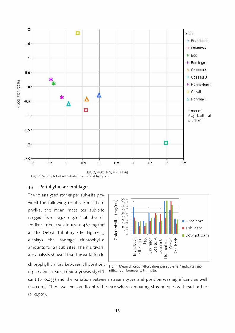
By looking only at the scores of all tributaries (Fig. 12), there is some grouping visible. All natural

and agricultural tributaries are clustered in two groups, whereas urban tributaries are scattered

over the whole score plot.

Discharge ratio (upstream /tributary)

Brandbach: 3.7

Effretikon: 11.2

Egg: 12.4

Esslingen: 2.8

Gossau A: 2.1

Gossau U: 1.3

Hühnerbach:7.6

Oetwil: 3.2

Rohrbach: 5.8

Fig. 9: Score plot of all positions separated by sites; Discharge ratio shown in the legend gives an indication of possible tributary effects.

15

* natural ∆ agricultural □ urban

Fig. 10: Score plot of all tributaries marked by types

Fig. 11: Mean chlorophyll-a values per sub-site; * indicates sig-nificant differences within site.

3.3 Periphyton assemblages

The 10 analyzed stones per sub-site pro-

vided the following results. For chloro-

phyll-a, the mean mass per sub-site

ranged from 103.7 mg/m2 at the Ef-

fretikon tributary site up to 467 mg/m2

at the Oetwil tributary site. Figure 13

displays the average chlorophyll-a

amounts for all sub-sites. The multivari-

ate analysis showed that the variation in

chlorophyll-a mass between all positions

(up-, downstream, tributary) was signifi-

cant (p=0.033) and the variation between stream types and position was significant as well

(p=0.005). There was no significant difference when comparing stream types with each other

(p=0.901).

16

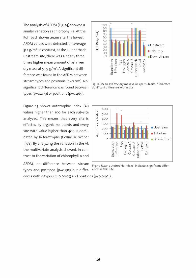
The analysis of AFDM (Fig. 14) showed a

similar variation as chlorophyll-a. At the

Rohrbach downstream site, the lowest

AFDM values were detected, on average

31.1 g/m2. In contrast, at the Hühnerbach

upstream site, there was a nearly three

times higher mean amount of ash free

dry mass at 91.9 g/m2. A significant dif-

ference was found in the AFDM between

stream types and positions (p=0.001). No

significant difference was found between

types (p=0.079) or positions (p=0.469).

Figure 15 shows autotrophic index (AI)

values higher than 100 for each sub-site

analyzed. This means that every site is

effected by organic pollutants and every

site with value higher than 400 is domi-

nated by heterotrophs (Collins & Weber

1978). By analyzing the variation in the AI,

the multivariate analysis showed, in con-

trast to the variation of chlorophyll-a and

AFDM, no difference between stream

types and positions (p=0.315) but differ-

ences within types (p=0.0005) and positions (p<0.0001).

Fig. 13: Mean autotrophic index; * indicates significant differ-ences within site

Fig. 12: Mean ash free dry mass values per sub-site; * indicates significant difference within site

17

Tab. 3: Table showing all sepcies found in the samples; Values stand for: 1 sporadic, 2 seldom, 3 regularly, 4 frequent, 5 dominant; Site codes: Eg = Egg, Ro = Rohrbach, GA = Gossau A, GU = Gossau U, Es = Esslingen, Oe = Oetwil, Br = Brandbach, Hü = Hühnerbach, Ef = Effretikon; Number coded: 1 = Downstream, 2 = Tributary, 3 = Upstream.

The algal taxonomic composition analysis conducted is shown in table 3.

Diato

meen

Eg1

Eg2

Eg3

Ro1

Ro2

Ro3

GA

1G

A2

GA

3G

U1

GU

2G

U3

Es1

Es2

Es3

Oe1

Oe2

Oe3

Br1

Br2

Br3

Hü1

Hü2

Hü3

Ef1

Ef2

Ef3

Achnanthes m

inutissima

33

32

22

23

23

33

22

22

22

23

34

33

43

4

Am

phora ovalis1

11

11

12

12

11

21

1

Am

phora pediculus2

22

22

22

12

32

33

22

34

42

33

33

3

Cocconeis placentula

11

11

24

22

22

21

23

32

23

31

32

3

Cym

bella affinis2

11

11

1

Cym

bella minuta

11

12

12

32

22

23

2

Diatom

a mesodon

23

21

11

Diatom

a vulgare3

33

23

44

34

33

44

44

43

34

32

33

3

Fragilaria ulna

31

23

23

43

43

34

43

24

44

33

32

22

21

1

Frustulia vulgaris

21

11

2

Gom

phonema olivaceum

33

42

11

43

44

34

34

43

32

23

22

22

23

Gyrosigm

a accuminatum

13

11

11

11

11

2

Melosira varians

11

22

21

22

22

33

22

22

21

31

Meridion circulare

21

11

21

23

23

11

11

11

1

Navicula exigua

44

44

43

32

22

23

33

34

33

31

33

12

32

Navicula sp.

32

22

22

12

22

12

23

33

44

43

33

34

Navicula pupula

33

42

33

33

33

13

33

22

22

22

Navicula radiosa

33

31

32

22

22

Navicula tripunctata

44

44

43

43

33

34

33

33

23

33

34

33

33

4

Nitzschia dissipata

33

33

33

33

32

23

23

32

22

23

33

33

33

4

Nitzschia linearis

11

11

11

11

11

11

21

21

12

12

2

Nitzschia palea

44

43

32

33

32

22

22

22

21

12

13

1

Rhoicosphenia abbreviata

21

23

23

22

22

21

13

42

31

33

23

22

Surirella linearis

11

Surirella brebissonii

11

11

22

21

12

12

23

21

11

12

Gom

phonema accum

ainatum1

11

Diploneis ovalis

11

11

oth

er algae

Lyngbya2

11

11

11

22

22

22

2

Trentepholia

1

Ulothrix

21

11

11

11

12

Cladophora

11

31

1

18

The most common species detected in the samples were Achnanthes minutissima, Fragilaria

ulna, Gomphonema olivaceum, Navicula exigua, Navicula tripunctata and Nitzschia dissipata.

All these species appear in every sample and mostly with high abundance. As this data is semi-

quantitative, there is no information

available regarding total numbers of

cells. Nevertheless, species richness can

be calculated and this is shown in figure

16. Species richness shows similar values

for nearly all sites. Most of the sites have

a species richness between 15 and 20 or

even higher. Lower values were detected

only at the Egg tributary (12) and down-

stream (14) sub-site and also at the Rohr-

bach downstream (12) sub-site.

Comparing all the biological data, there are some correlations visible (Fig. 17). Ash free dry mass

and chlorophyll-a show a positive correlation (r=0.79). Thus the more AFDM detected, the more

chlorophyll-a is present. Another interesting interaction can be seen between chlorophyll-a and

Fig. 15: Correlation matrix comparing species richness, ash free dry mass, chlorophyll-a and autotrophic index; all values are log(x+1) transformed.

Fig. 14: species richness of diatoms per sub-site.

19

the autotrophic index. This negative correlation (r=0.66) shows that the AI (AFDM/chlorophyll-

a) is driven by the amount of chlorophyll-a in the system and not by the amount of AFDM pre-

sent.

4 Discussion

As shown in the chemical analysis, there was little difference between the different kinds of

sites and land use types. Even by comparing tributaries and mainstem (up-, downstream) sub-

sites separately, no significant differences in physico-chemistry were found. Only some sites,

regardless of their land use characterization, had significantly higher concentrations of some

chemical components. The fact that these high concentrations were always from the up- and

downstream sub-site makes it impossible to determine the source because of the high varia-

tion in the inputs to the mainstem sites.

Despite the lack of significant differences between site categories, the tributary PCA score plot

showed quite nicely that the natural and agricultural tributaries are driven similarly by the

same principal components. The variation in urban scores are on the one hand due to a high

concentration of DOC and NO3-N at the Gossau U tributary sub-site and on the other hand due

to a high concentration of PO4-P at the Oetwil tributary sub-site. At Gossau U, we know that a

wastewater treatment plant is situated some hundred meters upstream of our sampling site,

and this probably explains the high levels of DOC and NO3-N.

Importantly, we must take into account that all sampling and measurements were conducted

in winter. At this time of year, the agricultural areas were not in use and probably reduced the

probability of a significant influence from these tributaries. Conducting the study in spring or

summer would likely have shown more tributary effects than results from winter. For example,

after applying fertilizer such as liquid manure on the fields, chemical conditions in agricultural

tributaries would have more pronounced than those in natural tributaries. Also, the winter in

2009/2010 had some strong ice periods in which a lot of salt was applied to roads. This may

explain the high conductivity values at Gossau U tributary sub-site. Gossau is one of the largest

settlements in the Mönchaltdorfer-Aa area and has many roads that were treated with salt.

As for the biological aspects, we cannot expect major differences between tributaries of differ-

ent land use types. As mentioned, periphyton communities reflect the water quality and gen-

eral health of aquatic ecosystems (Vis 1997), but since the chemical conditions of tributaries

were similar between the different land use types we can expect little variation in periphyton

assemblages (especially in winter). For instance, there was indeed no significant differences in

the amount of chlorophyll-a and AFDM between the land use types. Only the autotrophic index

20

(AI) showed significant variation between streams of the different land use types. The Ef-

fretikon and Egg tributaries showed, for example, AI values around 500. Therefore, we expect

that they are highly impacted by organic pollutants. But when looking at the chlorophyll-a and

AFDM values of these two sites, we see low values of AFDM, which is unexpected if they were

dominated by heterotrophs. The AI scores reflect the low chlorophyll values at these sites. One

explanation could be that, for example, at the Egg tributary sub site the riparian vegetation

mainly consisted of coniferous forest that absorbs a certain amount of light also in winter in

addition to the already low radiation input due to the time of year. The tributary also flows

through a basin with a high amount of natural shading that reduces radiation inputs to the

stream. At the Effretikon sub-site, a similar situation of riparian vegetation and landscape form

could be the reason for the low chlorophyll-a values.

The taxonomic composition can be described as being homogenous among all sites, types and

positions. There were no species present or absent in specific tributaries with a certain land use

type. This low variation in assemblage structure can also be explained by the similar chemical

conditions at all sites. The occurrence of certain species at only two or three sub-sites was al-

ways accompanied with a very low counts of individuals. For example, Surirella linearis, Gom-

phonema accumainatum, Diploneis ovalis and, as an example for a filamentous alga, the genus

Trentopholia only occured at a maximum of three sites with a occurrence value of one, which

means sporadic abundances. They may occur at other sites as well but were not detected in

samples due to very low counts.

In general, we can say that for hypothesis one:

- Periphyton community structure differs between different kinds of land use types in terms of

biomass, chlorophyll-a and taxonomic composition- was not supported as no differences were

found for any of the tested parameters.

For the second hypothesis:

- Tributary affects on periphyton community structure in mainstem river systems depends on

the dominant land use in the catchment- is partially supported.

The amount of chlorophyll-a and AFDM often shows a certain pattern in which the tributary

had higher values then the respective up- and downstream sub-site. However, the downstream

sub-site also had a higher value than the respective upstream sub-site. This suggests an in-

crease in chlorophyll-a and AFDM due to a tributary influence. This can be explained by the in-

put of nutrients into the mainstem that increases the overall productivity of the system down-

stream of the confluence. For example, the Gossau U tributary sub-site was significantly differ-

ent from the mainstem sub-sites in both chlorophyll-a and AFDM, and increased the mean

21

chlorophyll-a value to about 18.6 mg/m2 and the mean AFDM to about 195.6 mg/m2 from up- to

downstream.

In contrast to this pattern, there are some sites that show the opposite relationship. The most

extreme example is the Brandbach site. Here, the amount of chlorophyll-a detected between

the up- and downstream sub-site varied by a factor of two. This drastic reduction of chloro-

phyll-a from a mean value of 385.3 mg/m2 to 190.2 mg/m2 and AFDM from 91.8 g/m2 to 45.5

g/m2 could be due to harmful substances brought in by the tributary that reduced the overall

abundance of periphyton in the mainstem. However, this idea needs further study to make any

concrete conclusions.

5 Conclusion

This study did not show any differences in chemical conditions and periphyton community

structure between tributaries draining different kinds of land use areas. Only the autotrophic

index showed a significant difference between different types of sites. But even this evidence

can be explained by factors other than land use, namely riparian vegetation and suboptimal

geological conditions leading to very low chlorophyll-a values and therefore a high AI. So, the

first hypothesis must be rejected. As for the second hypothesis, there were patterns visible that

could be seen as indicators suggesting tributaries influence the mainstem by increasing the

overall productivity of the system. But having sites that show exactly the opposite behaviour,

by reducing the productivity of the mainstem further downstream, leads to the conclusion that

further analysis focusing on these effects needs completed. Also, the time of the year (season-

ality) should be taken into account. For example, the study should also be completed in

spring/summer when the effects of land use may be more clear.

Acknowledgements

I' thank Anna Streit and Martina Blaurock for their support during the field work and laboratory

analysis. Rosi Siber from EAWAG delivered very nice GIS data, for that I am very grateful. Thank

you Regula Illi for the time invested to analyse the periphyton taxa composition. Last but not

least, a big thanks to Christopher Robinson. He gave me the opportunity to do my master thesis

in the Eco department at EAWAG, Dübendorf, and supported me whenever he could. Thanks a

lot!

22

6 References

Azim, M. E. (2005). Periphyton: ecology, exploitation, and management. CABI Publishing, Ox-

fordshire UK.

Hynes, H. B. N. (1975). The stream and its valley. International Association of Theoretical and

Applied Limnology 19: 1-15.

Larned, S. T. (2010). A prospectus for periphyton: recent and future ecological research. Journal

of the North American Benthological Society 29: 186-206.

Rice, S. P., Greenwood, M. T., Joyce, C. B. (2001). tributaries, sediment sources, and the longitu-

dinal organisation of macroinvertebrate fauna along river systems. Canadian Journal of Fishe-

ries and Aquatic Sciences 58: 824-840.

Vannote, R. L., Minshall, G. W., Cummins, K. W., Sedell, J. R., Cushing, C. E. (1980). The river conti-

nuum concept. Canadian Journal of Fisheries and Aquatic Sciences 37: 130-137.

Vis, C., Cattaneo, A., Hudon, C. (2008). Shift from chlorophytes to cyanobacteria in benthic ma-

croalgae along a gradient of nitrate depletion. Journal of Phycology 44: 38-44.

Vymazal, J. (1987). The use of periphyton for nutrient removal from waters. British Phycological

Journal 22: 313-314.

Ward, J. V., Stanford, J. A. (1983). The serial discontinuity concept of lotic ecosystems. Dynamics

of lotic systems. Ann Arbor Science, Ann Arbor. p: 29-42.

6.1 Internet links

Link 1: http://www.nrp61.ch/E/Pages/home.aspx (25. 7. 2010)

Link 2: http://www.eawag.ch/organisation/abteilungen/uchem/schwerpunkte/iwaqa/index

(25.7. 2010)

23

6.2 Figure references

Fig. 1, 2: Maps from GIS, Data given by Rosi Siber

Fig. 4: Picture taken by Michael Scheurer

Fig. 11, 12, 16: Graphs generated with JMP (SAS).