ICES Journal of Marine Science, 58: 123- 136. 2001 ® doi:l0.1006/jmsc.2000.0996, ava ilable online at http://www.idealibrary.com on IDE~l

#

Effects of in situ target spatial distributions on acoustic density estimates

J. Michael Jech and John K. Horne

Jcch, J. M .. and Horne, J. K. 2001. Effects of in situ target spatial distributions on acoustic density estimates. ICES Journal of Marine Science, 58: 123- 136.

One goal of acoustic-based abundance estimates is to accurately preserve spatial distributions of organism density and size within survey data. We simulated spatially­random and spatially-autocorrelated fish density and cr0, distributions to quantify variance in density, abundance. and backscattering cross-sectional area estimates, and to examine the sensitivity of abundance estimates to organism spatial distributions and methods of estimating acoustic size. Our results show that it is difficult to simul­taneously estimate fish density and maintain accurate crbs· frequency distributions. Among our acoustic backscatter estimation methods. a weighted-mean from a local search window provided optimal estimates of density, abundance and crbs· Other methods tended to bias either crh, or density estimates. This analysis identifies the relative importance of variance sources when estimating organism density using spatial ly-indexed acoustic data.

Key words: density estimates, spatial modeling, underwater acoustics.

Received 9 November 1998; accepted 13 November 2000.

J. M. Jech. and J. K. Home: Coopera/il'e Institute for Limnology and Ecosys1e1n Research. Unil'ersity of Michigan, and NOAA-Great Lakes Enl'ironnumtal Research Laboratorp, 2205 Commonwealth Blvd., Ann Arbor, MI 48105, USA. J. 11tf. Jech: Presem address: Northeast Fisheries Science Cmter, 166 Water Sr .. Woods Hole, MA 02543, USA . .!. K. Home: Present address: Unil·ersity of Washington and NOAA Alaska Fisheries Science Center. 7600 Sand Poim WayNE. Bldg. 4, Seaule, WA 98115, USA. Correspondmce to .!. M . .!ecll: tel: (508) 495 2353; fax: (508) 4952258; e-mail: michael.jech@Jwaa.go1'

Introduction

Underwater acoustic technologies are non-invasive sampling tools commonly used to map distributions of fish and zooplankton abundance. density, and size. Advances in hardware and computing technology have increased the spatial resolution of acoustic data, thereby improving the ability to examine organism distributions at multiple scales (e.g. Horne and Schneider, 1997), to investigate predator- prey interactions (Levy. 1991 ), biological- physical interactions (Nash et a/., 1989; Megard et al., 1997), or use in bioenergetic modeling (Luo and Brandt, 1993; Brandt and Mason, 1994). Goals of fisheries acoustics arc to provide accurate abundance estimates and to preserve spatial distribu­tions of organism densities and sizes within survey data.

dimensional arrays where each array dimension is par­titioned into cells to maintain the spatial heterogeneity observed in organism distributions. Each cell contains volume backscatter integrated over the dimensions of the cell [i.e. integrated echo (Dragesund and Olsen, 1965; R0ttingen, 1976; Foote, I 978)] and backscattering cross-sectional areas (<>bs) of individual targets. Assum­ing that backscatter from targets is incoherent and linearly additive (Foote, 1983), numeric density is the total energy returned from a sample volume. divided by the energy from a representative scatterer within that volume (Medwin and Clay, 1997).

Spatially-explicit analysis formalizes methods for extracting quantitative spatiotemporal information from acoustic data (Brandt et a/., 1992; Mason and Brandt, 1996). Acoustic data are stored and analyzed in two-

1054-3139/01/010123 + 14 535.00/0

( 1)

where Pv is the density estimate [number m - 3], Sv is

vertically integrated and horizontally averaged volume backscatter over the spatial dimensions of the array cell, and &bs is the representative acoustic backscattering cross-sectional area (Figure I).

124 J. ll. Jt>ch and J. K Horne

(b)

Sv=w, Sv = Icr·? Sv = !cr., + !cry Sv =0 Sv=Lo'p

{> = Sv/o_. {> = Svla {> = Sv/o p=O {> = Svlap

Sv = !cr? Sv=Lo'? Sv = !cr·, Sv = !cry+ Iap Sv =0

{> = Sv/cr p = Sv/o {> = Sv/o p = Sv/cr p=O

Sv = !cr• Sv = l:a? Sv = :!:cr? + l:op Sv =Loy+ !crp Sv = !cr>'

{> = Sv/o p = Sv/cr p = Sv/cr {> = Sv/cr p = Svlav

Figure I. Acoustic cchogram and corrc,ponding spatially-mdc\ed arra~. The top schematiC (a) represents potential distributions of aquatic orgamsms obscrn:d along acoustic transect:.. Oat;t arra) (.'ells can contain resohcd indl\iduab of single or multiple ~pecics. no resolvable indi' idual targets (i.e. fish aggr.:gation). or may contain dillerent sJX>ciCs. siLes and scattering I) pes. The bottom schematic (b) shows the corresponding spatiall) mde.xed arnt). oP. <1>. cr, are acoustic bad.scattcring cross-sections of predators. pre), and 7ooplankton. respectively. 6. p arc the estimated backscatter and estimated density. and s, is \olume scattering. a.1 represents cells without resolvable individual targets. In cells with volume scattering and no resolved targets, a crh, must be estimated.

Selections of crh, arc critical for accurate density estimates. Strategies to choose a representati,·c acoustic backscattering cross-section can be grouped in two general categories: in situ targets. and acoustic catch relationships. In this paper. we focus on utilizing in si111 targets for calculating numeric density estimates within acoustic data arra; cells. In situ targets are acoustically resolved individuab using single- (Craig and Forbc~.

1969), dual- (Ehrenberg and Torkelson, 1996) or split­beam (Foote et at .. 1986; Soule eta/., 1996; Demer eta/., I 999) hardware and analyses.

We simulated ~patially-random and spatially­correlated fish densit)' and backscattering strength distributions to examine the influence of spatial di~tri­bution. crb,-frequenc~ distribution. and strategie~ used to estimate crh, on the accuraC) of density and

abundance estimates in sratially-indcxed acoustic data using in situ targets. These simulations represent methods for interpolating bachcattcring cross-section e~timatcs into sampling volume~ where individual targets are not detected. It ts important to note that \\e are not simulating techniques for reliable measures of individual targets, but invc~tigating how to use in sifll data for reliable estimates of organism density and abundance. Our specific questions are: does the crb,­frcquency distribution of a fish population aJTect accu­racy of density and abundance; does decreasing numbers of in situ targets affect accuracy of fish density and abundance estimates, and does the spatial distribution of fish densit; and backscattering strength alfect accuraq or demit) and abundance estimates?

Effects (!fin situ target spatial distributiom 011 acoustic de11sit_r estimate.\ 125

Materials and Methods

Simulated spatial dist ributions of fis h densities and sizes were designed to reflect fis h distributions commonly observed with underwater acoustics in a variety of freshwater and coastal ecosystems. Two discrete cat­egories of spatially-correlated data were used in simu­lations: random and autocorrelated. Four spatial distributions were simulated (Table I): (1) random­density and random-oh, (Random Distribution), (2) random-density and autocorrelated-ob, (Dispersal Layers). (3) autocorrelated-density and random-o1,_

(Mixed Aggregations), and (4) autocorrelated-density and autocorrelated-00 , (Discrete Aggregations). The Random Distribution simulates heterogeneous combi­nations of backscattering strengths within cells. where densities and o1"'s are independent among cells. Dispersed Layer simulations emulate a two layer distri­bution with a dominant fish site in each layer. Thb structure is analogous to two thermally segregated species. Mixed Aggregation simulations model crepuscular periods \\hen different fish species and si7cs co-occur. Discrete Aggregation simulations arc potentially the most realistic. simulating patchy distributions of similar sized fish within each patch.

Array generation

All simulations use a 200 x 200 array (40 000 cells) with a known number of fish per cell (density). and a known length and obs for each fish. To facilitate comparison among simulations and cr~ estimation methods. fish abundances were kept as consistent as possible among simulations (Table I). Four length-frequency distribu­tions: normal unimodaL normal bimodal. Poisson uni­modal, and Poisson bimodal were generated to populate the array (Figure 2). Mean and standard deviations of these length-frequency dist ri butions (Table I) were based on October 1996 survey data from Lake Ontario. Fish lengths were converted to ob, using an equation derived by Foote (1987). and the conversion from fish length to obs is assumed to represent the "true" length­frequency distribution. Random selections were chosen using a pseudo-random number generator from IDL (Interactive Data Language, Research Systems Inc .. Boulder, Colorado. USA).

Random distribution: spatially-random density and crhs distributions

Spatially-random distributions of fish densities and oh,'s for the Random Distribution simulation were obtained by randomly filling 79' ' " of array cells with fish densities. fish lengths and corresponding backscattering cross­sections (upper left paneL figure 3). Cell densities were randomly chosen from a Poisson distribution with the

mean equal to 1.55. Resulting cell densities ranged from 0 10 fish per cell. Fish lengths were randomly chosen from the four length-frequency distributions depending on sim ulation (Table 1), converted to o1", and then randomly placed in cells throughout the array.

Dispersed layer simulations: spatially-random density and spatially-autocorrelated ob, distributions

Spatially-random density distributions in Dispersed Layer simulations were chosen as in Random Dbtribution simulations. Spatially-autocorrelated obs dist ributions were obtained by using only bimodal length-frequency distributions. In the upper portion of the array, fis h lengths were random ly chosen from the smaller length-frequency mode to represent prey-sized fish. In the lower portion of the array. fish sizes were randomly chosen from the larger length mode to represent predator-sized fish (Figure 2).

Mixed aggregation simulations: spatially-autocorrelated density and spatially-random crb, distributions

Spatia lly-autocorrclatcd densities in Mixed Aggregation simulations were produced by krigi ng. Kriging is a statistical technique that estimates one- or two­dimensional covariances in spatially-indexed data (Crcssie. 1991 ). Estimating spatial variance in fish distri­butions is an example of the forward approach for obtaining abundance estimates using acoustic transect data (e.g. Petitgas. 1993). We used an inverse approach (~imilar to Simmonds and fryer, 1996) to produce a denstty map with specified variance and autocorrelation. A spherical variance model was used to krig fish densi­ties with the parameter values: range=26, nugget=O, and sill=3 (Table l). Patches arc defi ned using the range parameter, where cells within a radius of 26 cells from the center cell arc autocorrclated. The nugget parameter defines the amount of randomness in the data. The nugget was set to zero in Random Distribution and Dispersed Layer models to stmulate random density dtstnbutions. The sill parameter defines variabilit) withm a patch. Center cells for 85 patches were ran­domly chosen, and an additional ISO cells along a single row were designated as a layer. Initial fish densities for each patch were randomly chosen from a Poisson distri­bution with a mean of 2.15 (0 8 fis h per cell ). A mean of 2.15 generated fish abundances similar to those used in random density simulations. Initial cell densities within the layer were set to the maximum density of eight fish per cell.

The array containing these initial patch and layer cells wa~ kriged using the spherical model to produce an array with autocorrelated densit)' structure (lower left

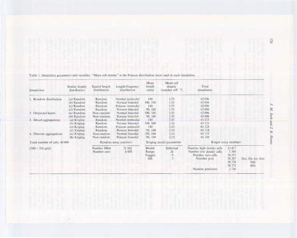
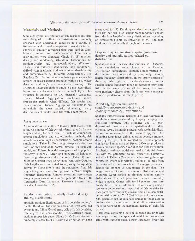
Table I. Simulation parameters and variables ... Mean cell dcnsit) .. is the Pois,on distribution mean used in each simulation.

Spalla! density Spatial length Lcngth-rn:quency Simulation tli~tribution distribution distribution

I. Random distribution (a) Random Random Normal unimodal (b) Random Random l\ormal bimodal (c) Random Random P()lsson unimodal (d) Random Random Po1sson bnnodal

2. Oispe~d !aye~ (a) Random "on-random 'slormal bimodal (b) Random 'Jon-random P()l\sOn bimodal

3. Mi'led aggregations (<~) Kngmg Random 's:ormal unimodal (b) Knging Random l\ormal bimodal (c) Kriging Random Poi-,son unimodal (d) Knging Random P01sson bimodal

4. Discrete aggregations (a) Kriging Kon-random Normal bimodal (b) Kriging Non-random Poisson bimodal

Total number or cells: 40 000 Random array ntnnb.:rs

(200 x 200 grid) Number filled J 1 542 !\umber zero 8 458

Mean Mean cell length density (mm) (number cell '>

140 1.55 100, 160 1.55

140 1.55 90. 160 1.55

100. 160 1.55 90. 160 1.55

I .tO 2.15 100, 160 2.15

140 2.15 90. 160 2.15

100. 160 2.15 90, 160 2. 15

Kriging model parameters

Model: Spherical Range: 26 Nugget: 0

Sill: 3

Total abundance

62 ()9(,

62 096 62 096 62 096 62096 62 096 61 123 61 123 61 123 61 114 61 123 61 108

Krig.:d array numbers

Number high dcn;,ity cells Number low density cclb

Number ;cro cells 1'\umber prey

'slumber predators

12417 I 368

26 215 58 387 58 378 58 372

2 736

3(a). (h). (c). 4(a) 3(d) 4(b)

Effects of in situ target spatial distributions on acoustic density estimates

Normal Unimodal Distribution 25000 .----------------------------.

20 000 II

0

Normal Bimodal Distribution 15000 .----------------------------.

10 000 -

5000

~ o~--~•~•~·~·~~~~~-~~----~~----~ Q Q)

g. Poisson Unimodal Distribution ~ 15000 .----------------------------.

10 000 -

5000 - h o L____.-.llj ......... ti ............. U 111 ..... ___ ._1____,

Poisson Bimodal Distribution 15 000

0 10 20 Length (em)

30 Backscattering cross-section (<Jbs m-2)

127

1 X IQ-4

Figure 2. Length-frequency distributions of fish populations used in simulations. Bimodal distributions are formed by joining two unimodal distributions. Mean and standard deviations for each distribution are listed in Table l.

128 J .V. Jec/1 und J K 1/ome

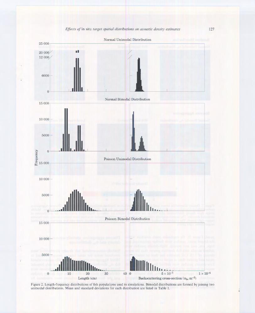
Random Distribution

Xormall"nimodal Ob.; distribution 95~ target removal Nearest neighbour fill method

Discrete Aggregation

Normal Bimodal Oh.• distribution 95% target removal Local-window fill method

Density (number cell 1)

0 8

2 4 6

Figure 3. Density distribution arrays used in Random Distribution (random-density/random-length) and Discrete Aggregation (autocorrclated-density/autocorrelatcd-length) simulations. Arrays on the left ~how the original density d istributions. Middle arrays show density distributions after 95% of the cells with targets arc removed. Right-hand arrays show the distributions of estimated densities. The nearest-neighbor estimation method creates artificial spatia l structure from random density distributions (upper right panel). The window-fill method preserved the original spatial density structure. even with low numbers of individual targets (lo,~er right panel).

panel. figure 3). To emphasize patch structure within the kriged array. patches were further categorized into high. low. and zero density. High-density patches were defined a~ celb with fish densities greater than the mean density of 2.15. Cell densities less than or equal to the mean and greater than or equal to zero were set to zero. LO\\-density patches were defined by setting cells with negatl\c densities to a fish density of two.

In mt'<ed aggregation simulations. fish lengths were randomly chosen from length-frequency distributions (Table I). converted to (jb,, and randomly placed in cells throughout the array. independent of patch density.

Discrete aggregation: spatially-autocorrelated density and crb, distributions

Spatially-autocorrelated fish density distributions were simulated u~ing the same kriging process outlined in \11 ixed Aggregation simulations. Spatially-autocorrelated fish crt> distributions were obtained using only bimodal length-frequency distributions. Prey aggregations were simulated b> placing smaller fish in high density patches and the layer. Isolated predators were simulated by placing larger fish in low density patches. and predator abundance was lower than in other simulations.

E./fecrs of in situ rarget spa rial distrihwions on acouvric demity estimares 129

crb, estimation methods

Estimating density within array cells requires a represen­tative crt>, in each cell. Foote (1983) suggested that a weighted-mean backscattcring cross-sectional area (crt>J be used as an estimate of crt>, when targets within a sampling volume arc of similar type (e.g. swimbladdered fish) and in sufficiently large numbers. In cells with one or more individual targets, a weighted­mean crb, of targets in each cell was used as the represen­tative backscatter. Tn cells with no individual targets, but with non-zero volume scattering (e.g. fish aggregations with no resolvable targets), crb• was estimated using ( 1) a weighted-mean from the distribution of individual targets in the full array. (2) a weighted-random choice from the distribution of individual targets in the full array, (3} a weighted-mean from the distribution of targets within a local-search window, and (4) a nearest neighbor.

The weighted-mean estimation method uses a mean crb, from all individual targets throughout the array weighted by the frequency of occurrence. This mean backscatter is used as the representative crbs in all cells \\ith non-1ero volume backscattering but with no indi­vidual targets. The weighted-random estimation method chooses a representative backscatter from the distribu­tion of all indiYidual targets in the full array. Random choices are weighted by the frequenq of occurrence and a ne\\ crh, is chosen for each cell. The local-windov. estimation method searches for individual targets by beginning with array elements immediately surrounding a cell, and then increases the search radius until either a minimum number of targets is found or a maximum window size is reached. Three window parameters: maximum window radius, window shape, and minimum number of targets define the search pattern and target criteria used to estimate a representative crbs· We used a maximum radius of 25 cells, a symmetric (i.e. square) shape, and a minimum of five targets within the search window. Search patterns may be varied from symmetric to elongated shapes to accommodate different spatial distributions of organisms such as layers or patches. A minimum number of targets within the search window provides a dbtribution of targets for crb, estimation and avoids duplicating the nearest-neighbor search strateg]. Setting a maximum window size restricts the search pattern to a local area where similar species are expected and aYoids searching the entire array. When the mini­mum number of targets is found, the weighted-mean of those targets is used as the representative crb,· If the maximum wtndO\\ site is reached and no indi,idual targets are found. cell density is set to zero. Setting cell densities to zero is used as a diagnostic in the simula­tions. In practice, these cells can be set to another choice of crb,· For the nearest-neighbor estimation method, the cr1" of the nearest target is used as the representative

&b,· If two or more targets are equidistant. then the weighted-mean of those targets is used as the representatiYe crb,·

.• Target removal

To simulate situations \\here indi,idual targets are not resolved, all targets were removed from randomly chosen cells while retaining the known volume back­scattering ("'otargct removal). %target removal is calcu­lated as the percentage of cells deleted from the array. It does not equal the percentage of individual targets removed, as a cell can contain more than one target. %target removal for each set of simulations was increased from s•y., to 95% in 5'Jio increments, and targets in remaining cells were used to estimate the represen­tative crb, in cells lacking individual targets. The removal of targets from random cells did not modify the crb,­frequency distributions in any simulation. After estimat­ing the backscattcring cross-section within each cell. cell densities were computed using Equation (I) and fish abundance was calculated. Accuracy of fish density and abundance estimates was quantified by computing de,iations between original (before target removal) and estimated data arrays.

De\·iation indices were calculated as a function of o,utarget remo\ al to test the accurac) of each crbs estima­tion method. Accuracy of abundance estimates was quantified using a normalited abundance deviation index

Ncelh "Jcells

I pi- I Pk; Abundance deviation index j w l i= 1

Ncells (2)

I Pk; i-1

where p is estimated density, Pk is known density in the i'11 cell before target removal, and Nccus is the total number of cells in the array (40 000). Because initial fish abundance~ were not equal in all simulaitons (Table 1). abundance deviations were normalized to facilitate com­parisons among simulations. Mean per-capita deviation indices for den~ity and 6-n, estimates were computed using

1 "«II< [ p - p . J Density deviation index=-, - I -' __ k,

Ncelh ; = 1 Pt; (3)

(4)

where crk is the known backscanering cross-sectional area, and cr is the estimated value. The value of Ncel~> differs among abundance, density, and crb, deviation indices. For abundance deviation indices, Nccns is the number of cells in the array. For density and crb, indices,

130 J. .\!. Jech and J. K. Horne

crb9-frequency distribution

I -o Q)

"' .... Q)

Q -~ .8 Ci

~ :::> rl) j] 0.050~--~ 0.50

Poisson Unimode

-o l ~~~~~~~~~

Normal Bimode

25 50 75 100

0.25

0 25 50 75 100 0.50 .-------

0.25 -~1

0.00~

Poisson Bimode

0 25 50 75 100

0 25 50 75 100

2 ·

:t::l j 0.025~: . . .. ~..HI 0.25 ,

-~ 0.000 0.00¢'

::2J 0 25 50 75 100 OL.,__2_5 ___,50 75 100 "'

0 25 50 75 100 0 25 50 75 100

§ % Targcl removal :;j

j B "' .... "' "' 0

%Target removal

::f, I 000~

0 25 50 75 100 '1 Target removal

0 25 50 75 100 'K Target removal

Figure 4. Mean pcr-capua dcnsit) de,·iation index as a function of 'X.target removal. ",otarget removal wa~ incremented in 5 'o steps. Column comparison~ illm>~rate the effect of using ditTercnt crb -frequency distribution>. RO\~ compam;ons illustrate the effect of using different crb, C>timation method> on density estimates. crn, e~timation methods are represented by: • - mean fill. V random fill, • local window. and-<>- nearest-neighbor.

Ncclls is the number of cells with targets removed and Ncdls increases as "1utargct removal increases. Positive deviation index values indicate overestimates, whilst negative values indicate underestimates of fish density, abundance, and bacl,scanering cross-sections. For abundance estimates, a de,iation index value of I is equivalent to a doubting in abundance.

Results Fish density, abundance. and 6-bs estimates were inOu­cnccd by the choice of crb,-frequency distribution in all simulations (Figures 4- 6). Density, abundance, and crh, estimates were most accurate using the normal unimodal distribution, whereas de\'iation indices were I 2 orders of magnitude larger \~ith the Poisson bimodal distribu­tion. This reduced accuracy rna} result from the wider range offish baekscattering cross-sections in the Poisson

distributions compared to the normal distributions. The local-window estimation method preserved spatial density structure in Discrete Aggregation simulations (bottom row Figure 3). The nearest-neighbor method created artificial structure from ~patially random dcnsit> distributions (top row figure 3).

Estimates of fish density (Figure 4) and abundance (Figure 5) using the local-window method were consist­ently more accurate than other crb, estimation methods for all spatial distributions and 0'b,-frequency distribu­tions. For all spatial distribution simulations and crb,­

frequency distributions, the random-fiJ I estimation method provided the least accurate density and abun­dance estimates (Figures 4 and 5). Using the nearest­neighbor method, density and abundance estimates were more accurate when density and ab, distributions were both spatially autocorrelated (Discrete Aggregations) than when spatial distributions were random (Figures 4

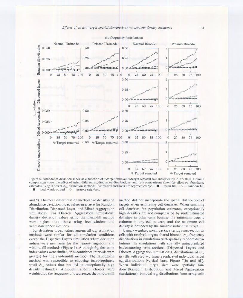
Effects of in situ target spatial distributions on acoustic density estimates 131

Ob0-frequency distribution

Normal Unimode Poisson Unimode Normal Bimode Poisson Bimode c 0 0.050 0.50 0.50 2 :.;; ~

..0

·~~ ·;: ...,

0.025 0.25 1 <f}

;a s 0 0 "0

0.000 0.00 0.00 c "' ~ 0 25 50 75 100 0 25 50 75 100 0 25 50 75 100 0 25 50 75 100 (I] 0.50 ... Q)

» ~ "0 1 Q) (I] ... Q) Q..

c.~ .~ Q ,_j

0 25 50 75 100 0 25 50 75 100 <1) ~ (I]

~ c 0.050 0.50 0.50

:~ e o ...... :a

Cl) Ol b.O Q) ... 0.25 ~ 0.025 < "0

"' 0.00 ~ 0.000

0 25 50 75 100 0 25 50 75 100 0 25 50 75 100 0 25 50 75 100 "' Q % Target removal 0.50 %Target removal 0.50 2 ·~ <ll I tl.O

"' 11 So 0.25 tl.O

0~ < $ ,..,._.. Q) 0.00 ... <) <f} ..... 0 25 50 75 100 0 25 50 75 100 0

% Target removal %Target removal

Figure 5. Abundance deviation index as a function of %target removal. %target removal was incremented in 5% steps. Column comparisons show the effect of using different ob,-frequency distributions, and row comparisons show the effect on abundance estimates using different &0• estimation methods. Estimation methods are represented by: - • mean fill, '1/- random fill. - • - local window, and -0- nearest-neighbor.

and 5). The mean-fill estimation method had density and abundance deviation index values near zero for Random Distribution, Dispersed Layer, and Mixed Aggregation simulations. For Discrete Aggregation simulations, density deviation values using the mean-fill method were higher than those using local-window and nearest-neighbor methods.

crb, deviation index values among all obs estimation methods were similar for all simulation conditions except the Dispersed Layers simulation where deviation indices were near zero for the nearest-neighbour and window-fill methods (Figure 6). Although crbs deviation index values were similar, 95% confidence intervals were greatest for the random-fill method. The random-fill method was susceptible to choosing inappropriately small cr bs values that resulted in exceptionally high density estimates. Although random choices were weighted by the frequency of occurrence, the random-fill

method did not incorporate the spatial distribution of targets when estimating cell densities. When summing cell densities for population estimates, exceptionally high densities are not compensated by underestimated densities in other cells because the minimum density estimate in any cell is zero, and the maximum cell density is bounded by the smallest individual target.

Using a weighted mean backscattering cross-section in cells with resolved targets altered bimodal crb,-frequency distributions in simulations with spatially random distri­butions. In simulations with spatially autocorrelated backscattering cross-sections (Dispersed Layers and Discrete Aggregation simulations), distributions of crbs in cells with resolved targets replicated individual target cr1"-distributions [vertical bars, Figure 7(b) and (d)). When individual target sizes were spatially ran­dom (Random Distribution and Mixed Aggregation simulations), bimodal obsdistributions from array cells

132 J . . \/. Jech and J. K Horne

Ot,,-frcqucncy distribution

,:: Normal Unimode Poisson Unimodc Normal Bimode Poisson Bimode

t0.050 1 -

i •-•'•l.!.J.~I -g o.oooft'i'f"Y·~ · -y

~

::: m!~~IOOOOOo<OOOO I ::: 1:::' 0.00

-'-----' 0.00 ~R 0 25 50 75 100 0 25 50 75 100 0 25 50 75 100 0 25 50 75 100

"' $ >. ~ "0

"' z; "' Q.,

d -~ .s 0 ~ :; ~ E o 0.050

Ci3 ·~ t:c

~ 0.025 ~

0.25

0 25 50 0.50--- - 0.50.-----

0.25 0.25 ..

2

1

0

75 100 0 25 50 75 100

2

1 ...

i o.ooo~l o.oo~ o.oo~ 0~ 0 25 50 75 100 0 25 50 75 100 0 25 50 75 100 0 25 50 75 100

(/) ,:: 0 ·.;;

j ~·Target removal %Target removal 0 50 -

.,. - .. _ _ _ _ _ _ I

0.00~

0 25 50 75 100 "k Target removal

0~

0 25 50 75 100 <k Target removal

Figure 6. \1ean per-capita a..,_ deviation index as a function of%target remo\al. "·.target rcrno\al was mcremented in 5" step-.. Column comparison-, ~ho'' the efrect of using different ah.-fn.:quenq distributions. and rO\\ compari>ons show the effect on ab, estimates using different C>timation methods. <i'bs estimation methods are represented by: e mean fill. -"'- random fill.

• local window. and - nearest-neighbor.

with resolved targets were altered to having greater numbers at the mean [vertical bars. Figure 7(a) and (c)). The local-window and nearest neighbor methods repli­cated the distribution of <J0 , \ rather than the original a~».·distribution of indi\ idual targets throughout the arra) when cr.,,-dbtnbutions were random (lower panel. Figure 7). The random-fill method retained the cr.,,­dbtributions of indiYidual targets for all simulation conditions. The mean-fill estimation method altered individual target crb,-frequency distributions to greatly increase numbers at the mean and reduce the number of GbsS at intermediate values and tails for a ll simulation conditions (Figure 7).

Discussion

We recommend the use of a local search window among crbs estimation methods examined. The local-\\ indO\';

method consistently gave accurate estimates of fish densities and array abundances. and preserved O't,_·

frequency distributions. The local-window method com­bines the nearest-neighbor and mean-fill methods by using the ·weighted-mean 0'0 , from a distribution of indiYidual targets in clO\e proximity to cells requiring an estimate of acoustic backscattering cross-section. Using a distribution of individual targets to choose a rcprcsen­tati\'C &0, reduces the probability of choosing an extreme value when estimating fish density. Since fish tend to aggregate with similar sized individuals of the same species (Ranta and Lindstrom. 1990; Ranta e1 a!., 1992). a local search pattern preserves spatial distributions by using contiguous targets to estimate crbs· Schooling and shoaling behaviors result in spatially-autocorrelated dis­tributions of fish den~itie~. species, and sizes. Tn our simulations. estimates of density and abundance were most accurate \\hen spatial distributions of den sit) and

E.lfect.\ of in situ target spatial cli!>tribwicm.\ 011 acoustic de11sity estimates 133

Random Distribution Dispersed Layers Mixed Aggregations Discrete Aggregations 20 000

~ (b) I (d) I (a) (c)

~ d

~ <ll 10000k :l C1" <ll

~

o I Normal Bimodal Distributions -------------------------------- -----------------------------95% Target Removal

ffi ::::: ~~ --l § 20 000/

~ 100: ,.._.,..,ll,.o.o,owd!""IOulwllliJiauo-,-----1

I *

. d.J .....

l ~

J ... 11

§ s 0

'"t) c <"¢

p::

.lh ....... llu •.

:?;

10 ooo I 0

'"t) d -~ 5000 -~ u

.3

0 I .Ill.

110000! II

i 5000

r II. oiU. r I I J r I Z O WUW.r- J 1.,_ ... 111.,. J 111,11111 ... I

0 1 X 10 ·6 2 X 10 -~ 3 X 10 ° J X 1Q-6 2 X 10·6 3 X 10-~ 1 X 10-5 2 X 10-5 3 X 10 r.

_j I. r-·_..._,_on I _______,,

t x tO 5 2x t o-G 3x 10-o

Backscattering cross-section (<Jbs m-2)

Figure 7. Backscattering cro>~-scction original and simulated frequency distributions after filling cclb or targ.:t removal. The top panel shows normal bimodal O"~n distributions of individual target> (solid lines) and the resulting crt>< distributions after array cells have been filled and the mean bacbcanering cross-sections have been calculated (vertical bars). The number of predators (larger cr.,. mode) is les:> in the Discrete Aggregation simulation' than in the Random Distribution. The bonom section shows backscattering cross-section di,tributions in array cells re:>ulting from the four estimation methods after 95% target rcmo,al.

134 J. M. Jec/z and J. K Home

backscattering cross-sections were autocorrelated. This is reassuring as spatially-autocorrelated distributions simulate discrete patches of fish typically observed in freshwater, estuarine, and marine environments.

Accuracy of fish density. abundance, and 6bs esti­mates declined when as little as 5% of known targets were randomly removed from the data set but did not decrease in proportion to the percentage of known targets removed. Density and crbs deviat ion index values remained fairly constant up to 95% target removal. suggesting that backscattcring cross-section estimation methods used in this study are not sensitive to the number of available targets. Insensitivity of density, abundance, and 6b, estimates to numbers of individual targets may be an artifact of randomly removing targets from the entire range of fish sizes. Even at 95% target removaL all modes from multimodal fish size dis­tributions were represented. Subsequent simulations would remove specified size classes in greater proportion to other size classes from multimodal frequency dis­tributions. As an example, prey fish that may not be acoustically resolvable within schools would be separated from predatory species that are resolvable.

Inclusion of backscattcring by different types of organisms will reduce the etTectiveness of in situ targets for density, abundance, and cr1, estimates by increasing the range of, and number of modes in backscattcring strength distributions. We simulated spatial distribu­tions of backscattering by organisms of similar acoustic scattering characteristics. Acoustic data collected in the field is comprised of backscatter by a number of physical and biological sources. Behavior and activity levels such as during crepuscular periods when fish vertically and horizontally migrate to feed (Ungar and Brandt. 1989; Levy, 1990, 1991; Boudreau, 1992), will also affect the accuracy of density estimates. Applying volume back­scattering and individual target thresholds wi ll reduce the amount of backscattering by non-swimbladdered organisms so that backscatter can be apportioned to swimbladder bearing fish. Varying cell size so that the spatial dimensions of array cells match aggregation dimensions may also increase the utility of in siw targets for density and abundance estimates. The strategy used to select representative backscatterers depends on the number of individual targets and the number of species present in a sampling area. Alternatives to using i11 situ targets include using length-frequency distributions from catch data. using species composition and length­frequency distributions from previously collected catch or acoustic data, or changing the time of sampling.

All simulations assume linearity of backscattering (Foote, 1983) from isolated individuals and from indi­viduals within aggregations. Furusawa et a!. (1992) calculated that attenuation effects on abundance esti­

mates were negligible below packing densities of approximately 0.8 fish m - 3 We have not simulated

backscattering from the dense schools where non-linear effects on sound transmission such as sound attenuation (R0ttingen, 1976) and shadowing (MacLennan and Simmonds, 1992) may be significant. Tn cases where the summation of backscatter is not linear, algorithms that quantify relationships between acoustic volume back­scattering and catch data must be used to ensure accurate density and abundance estimates of fish (Misund et at., 1992) and zooplankton (Hewitt and Demer, 1993). EITects of non-linear sound scattering from densely packed aggregations on fish density and population estimates can be minimized by collecting acoustic data when fish disperse and individual echoes are better resolved (Brandt eta!., 1991; Simmonds eta!., 1992).

Using in situ targets to estimate acoustic back­scattering cross-sections within aggregations assumes that species and crbs·frequcncy distributions of individ­ual targets match those of non-resolvable individuals within aggregations. This may not always be the case. Rose ( 1993) found that aggregations of migrating Atlantic cod (Gadus mor!tua) were structured by fish length. When individual targets are not available or not representative of individuals within aggregations, back­scattering cross-sections can be estimated using length­frequency data from net catches. Results of catch data- acoustic backscatter comparisons are commonly empirical regression equations describing the relation­ship between acoustic backscatter and individuals (e.g. Love, 1971; Midttun, 1984; Foote, 1987) or aggrega­tions (e.g. Love, 1975; Rudstam et at., 1987; Fleischer et al .. 1997) of fish or zooplan kton. Constrain ts to this approach are that catch data arc rarely available from the identical volume surveyed using acoustics. and that catch data arc size selective.

Tn our simulations, as well as when a mean back­scattering cross-section is derived from catch data, a distribution of backscattering strengths is characterized as a single value. Wide ranges and/or multimodal distri­butions of crbs may not be adequately characterized by a mean. An a lternate approach would use the distribution of crh:s to form a probability-density-function (PDF) of densities for each array cell. This density PDF may then be used to construct a distribution of population estimates, and potentially for size-based density and abundance estimates.

Quantifying variability in population abundance estimates requires an understanding of the variance at each step in the estimation process. Measurement errors in volume backscattering and variabili ty in individual acoustic backscattering measurements due to fish activity and orientation (e.g. Foote. 1980) or individual echo discrimination (e.g. Demer eta/., 1999) occur prior to placing acoustic data into spatial arrays. Variabili ty

d ue to survey or sampling design occurs after cell­based density estimates are made. The goals of these

Effects of in situ target spatial distributions on acoustic density estimates 135

simulations were to quantify variance in density esti­mates whilst retaining the spatial complexity of organ­ism distributions. This paper quantified variance associated with selecting a representative acoustic back­scattering cross-section from in sitll targets: extracting spatio-temporal information from acoustic data; and quantifying variability associated with estimates of density and organism size within spatially-indexed cells. In our simulations, the efficacy of backscattering cross­sectional estimation methods was not influenced by measurement or survey design variabili ty. Quantifying variances at each step of the population abundance estimation process allows partitioning of biases incurred when translating acoustic data to biologically and ecologically meaningful metdcs.

Acknowledgements

We thank the students (Darryl Hondorp, Dennis Roy. and Lian Zhou) and staff (Karen Barry, Eric Demers, Jiangang Luo, and Jeff Tyler) of the Great Lakes Center SUNY-College at Buffalo, and Lynn Herche of the NOAA-Great Lakes Environmental Laboratory, Ann Arbor, MI for insightful discussions on this problem. We would also like to thank Steve Brandt, Gordie Schwartzman and David Schneider for helpful com­ments on a presentation of a previous version of this work. Thanks to David Reid (Aberdeen, Scotland}, David Demer of the NOAA/NMFS-Southeast Fisheries Science Center, and one anonymous reviewer whose comments clarified this paper. This work was supported by NSF-LMER #032679 (Trophic Interactions in Estuarine Systems) (JMJ), the Office of Naval Research (NOOOI4-89J-1515) (JMJ, JKH), and the New York Sea Grant Institute (NA46RG0090) (JKH). This is GLERL contribution # 1203.

1) 200 I US Government

References

Boudreau, P. R. 1992. Acoustic observations of patterns of aggregation in haddock (Melanogrammus aeglefinus) and their significance to production and catch. Canadian Journal of Fisheries and Aquatic Sciences, 49: 23- 31.

Brandt. S. B., and Mason, D. M. 1994. Landscape approaches for assessing spatial patterns in fish foraging and growth. In Theory and Application in Fish Feeding Ecology. Ed. by D. J. Stouder, K. L Fresh, and R. J. Feller. BelleW. Baruch Library in Marine Science, #18.

Brandt, S. B., Mason, D. M .. Patrick, £. V., Argyle, R. L, Wells, L , Unger, P. A., and Stewart, D. J. 1991. Acoust ic measures of the abundance and size of pelagic planktivores in Lake Michigan. Canadian Journal of Fisheries and Aquatic Sciences. 48: 894- 908.

Brandt, S. B., Mason, D. M., and Patrick, E. V. 1992. Spatially­explicit models of fish growth rate. Fisheries, 17: 23- 33.

Craig, R. E., and Forbes, S. T. 1969. Design of a sonar for fish counting. Fiskeridirektoratets Skrifter Serie Havundersokelser, 15: 210- 219.

Cressie. N. 1991. Statistics for Spatial Data. John Wiley and Sons, Inc., New York.

Demer, D. A .. Soule. M. A., and Hewitt, P. R. 1999. A multiple-frequency method for potentially improving the accuracy and precision of in situ target strength measure­ments. Journal of the Acoustical Society of America, 105: 2359- 2377.

Dragesund, 0., and Olsen, S. 1965. On the possibility of estimating year-class strength by measuring echo­abundance of 0-group fish. Fiskcridirektoratets Skrifter Serie Havundersokclscr, 13: 47- 75.

Ehrenberg, J. E., and Torkelson, T. C. 1996. Application of dual-beam and split-beam target tracking in fisheries acoustics. ICES Journal of Marine Science. 53: 329- 334.

Fleischer, G. W., Argyle, R. L.. and Curtis, G. L 1997. In si1u relations of target strength to fish size for great lakes pelagic planktivores. Transactions of the American Fisheries Society. 126: 786- 794.

Foote, K. G. 1978. Analysis of empirical observations on the scattering of sound by encaged aggregations of fish. Fiskeridirektoratets Skrifter Serie Havundersokelser, 16: 423 456.

Foote, K. G. 1980. Effect of fish behaviour on echo energy: The need for measurements of orientation distributions. Rapports et Process-Verbaux des Reunions du Consei l International pour !'Exploration de Ia Mer, 39: 193- 201.

Foote, K. G. 1983. Linearity of fisheries acoustics, with addition theorems. Journal of the Acoustical Society of America, 73: 1932- 1940.

Foote, K. G. 1987. Fish target strengths for use in echo integrator surveys. Journal of the Acoustical Society of America, 82: 981 987.

Foote, K. G., Aglen, A., and Nakken, 0. 1986. Measurements of fish target strength with a split-beam echo sounder. Journal of the Acoustical Society of America. 80: 612- 621.

Furusawa, M., Ishii. K., and Miyanohana, Y. 1992. Allenua­tion of sound by schooling fish. Journal of the Acoustical Society of America, 92: 987- 994.

Hewitt, R. P., and Derner, D. A. 1993. Dispersion and abun­dance of Antarctic krill in the vicinity of Elephant Island in the 1992 austral summer. Marine Ecology Progress Series. 99: 29- 39.

Horne. J. K., and Schneider, D. C. 1997. Spatial variance of mobile aquatic organisms: capclin and cod in Newfoundland coastal waters. Philosophical Transactions of the Royal Society of London B Biological Sciences, 352: 633- 642.

Levy, D. A. 1990. Reciprocal die! vertical migration behavior in planktivores and zooplankton in British Columbia lakes. Canadian Journal of Fisheries and Aquatic Science, 47: 1755- 1764.

Levy, D. A. 1991. Acoustic analysis of dicl vertical migration behavior of Mysis relic/a and Kokanee (Oncorhynchus nerka) within Okanagan Lake, British Columbia. Canadian Journal of Fisheries and Aquatic Science, 48: 67 72.

Luo, J., and Brandt. S. B. 1993. Bay anchovy Anclwa mitchelli production and consumption in mid-Chesapeake Bay based on a bioenergetics model and acoustic measures of fish abundance. Marine Ecological Progress Series, 98: 223- 236.

Love, R. H. 1971. Measurements of fish target strengths: A review. Fisheries Bulletin, 69: 703- 715.

Love, R. H. 1975. Predictions of volume scattering strengths from biological trawl data. Journal of the Acoustical Society of America, 57: 300- 305.

136 J. M. Jech and J. K Horne

MacLennan, D . N .. and Simmons, E. J. 1992. Fisheries Acou~tics. Chapman and Hall, London. 325 pp.

Ma,on. D. M .. and Brandt. S. B. 1996. Effects of ~patial 'calc and foraging ellkicnq on the predictions made by 'patiall)-exphcit models of fish gro,Hh rate potential. Em iron mental Biolog) of F"hc:.. 45: 283 298.

Mcd\\ln, H .. and Clay. C. S. 1997. Fundamentals of Acou~tical Oceanography. Academic Press. N Y. 71 2 pp.

Megard, R. 0., Kuns, M. M .• Whi teside, M. C.. and Downing, J. i\. 1997. Spatial dist ributions of .woplank ton during coa,ta l upwelling in western Lake Superior. Limnology and Occanograph), 42: 827 &40.

\1Jdttun. L 1984. Fish and other oreanisms as acoustic targch. Rapports et Procc"-\'erbatL~ des Reunions du Con":il International pour f"Exploration de Ia Mer. 184: 25 -33.

Misund. 0. A., /\glen. A., Bcltestad. A. K., and Dalen. J . 1992. Rela tionships between the geometric d imensions a nd biomass of schools. ICES Journal of Marine Science. 49: 305 315.

'-Ja,h. R D. \L ~agnu:.on. J. J. Stanton. T. K .. and Clay. C S 19&9. Distribution of pcab of 70kH z acoustic scatter­mg 111 relation to depth and temperature during da) and night at the edge of the GulfStream-EchoFront 83. Dc:ep-Sea Research. 36: 587- 596.

Pet itgas, P. 1993. Geostatistics lor fish stock asscs!>mcnts: a review and an acoustic a pplicat ion. JCES Journa l of Marine Science. 50: 285-298.

Ra nta, E., and Lindstrom, K. 1990. Assortat ive schooling in three-spined ~ticklebacks? Annuales Zoologici Fenniei. 27: 67-75.

Ranta. E .. Lindstrom. K .. and Pcuhkun. '1. 1992. Size matters when thrce-~pined sticklebacb go to schooL \nimal Behaviour. 43: 160 162.

Rore. G. A 1993. Cod spawning on a migration highwa) mthc north-west Atlan tic. Nature. 366: 458-461.

R0ttingcn. L 1976. On the relation between echo in tcnsil)i and lish density. F iskeridi rcktoratcts Skrif'ter Scrie Havundcrsokclser, 16: 301-314.

R udstam. L G .. C lay. G. S .• and l\1agnuson. J . J . 1987. Density and >1/C estimates of cisco. Corcgonu> artedii using anal} sis of echo peak PDF froma single tran,ducer sonar. Canad1an Journal of F1,heries and Aquatic SCJt:nce. 44: 811 821.

Simmonds. E. J .. and Fryer. R. J. 1996. Which are bcuer. random or systematic acoustic surveys'! i\ simula tion using North Sea herring as an example. ICES Journal of Marine Science. 53: 39 50.

Simmonds, E. J., Williamson, N.J .. Gerlotto. F ., a nd Aglen. A. 1992. Acoustic survey design and analysis procedure: a compn:hcnsive review of current practice. ICES Cooperative Research Report #187. Copenhagen. Denmark. 128 pp.

Soule. l\.1. -\ .• Hampton. L and Barange. M. 1996. Potential impro,cmcnll> to current methods of recognizing single targets with split-beam echo-sounder. ICES Journal of Marine Science. 53: 237-244.

Unger, P. A., and Brand t, S. B. 1989. Seasonal a nd d ie! change:. in sampling conditions for acoustic surveys of fish a bundance in small lakes. f isheries Research. 7: 353 366.