EFFECTS OF HEAVY AGRICULTURAL VEHICLE LOADING ON PAVEMENT PERFORMANCE

A THESIS SUBMITTED TO THE FACULTY OF THE GRADUATE SCHOOL

OF THE UNIVERSITY OF MINNESOTA BY

JASON LIM

IN PARTIAL FULFILLMENT OF THE REQUIREMENTS FOR THE DEGREE OF MASTER OF SCIENCE

ADVISOR: LEV KHAZANOVICH CO-ADVISOR: JOSEPH F. LABUZ

JANUARY 2011

© JASON LIM 2011

i

Acknowledgements

My deepest gratitude goes to my advisor, Professor Lev Khazanovich, for his guidance

and willingness to convey unending knowledge and wisdom, both within and outside of

my academic pursuit. I wish to express my warm and sincere thanks to my co-advisor,

Professor Joseph Labuz, for his invaluable support and for providing me with the

opportunity to pursue my master’s degree here at the University of Minnesota. I am

grateful to Professor Douglas Hawkins, for his time and effort in reviewing my thesis and

for agreeing to serve on my exam committee.

To my many friends and colleagues who were and were not “assigned volunteers”

throughout the field testing of this research, I am indebted to you all. I am especially

grateful to Kyle Hoegh, Mary Vancura, Peter Bly, Priyam Saxena, Luke Johanneck,

Kairat Tuleubekov, Derek Tompkins, Madhavan Vasudevan, Simon Wang, and Andrea

Azary. I am particularly grateful to my undergraduate research assistant, Jacob Hanke,

for the large amount of time and effort spent on this research.

I would like to acknowledge the project sponsors: the Local Road Research Board, the

Professional Nutrient Applicators Association of Wisconsin, Iowa Department of

Transportation, Illinois Department of Transportation, Wisconsin Department of

Transportation, and Minnesota Department of Transportation. It has been an honor to

work with Dr. Shongtao Dai from the Minnesota Department of Transportation and I

would like to extend my appreciation for his expertise and advice.

Lastly, and most importantly, I wish to express my loving thanks to my family: to my

parents, Jerry Lim and Ann Kok for all their love and immeasurable support, and to both

my sisters, Sylvia Lim and Agnes Lim, for their continuous moral encouragement. To

them, I dedicate this thesis.

ii

Abstract

Agricultural equipment manufacturers have been producing equipment with larger

capacity to meet the demands of today’s agricultural industry. This rapid shift in

equipment size has raised concerns within the pavement industry, as these heavy vehicles

have potential to cause significant pavement damage. At present, all implements of

husbandry are exempted from axle weight and gross vehicle weight restrictions in

Minnesota. However, they must comply with the 500 lb per inch of tire width restriction

which may lead to very large loads as long as the tires are sufficiently wide.

A full scale accelerated pavement test was conducted at the MnROAD test facility. Both

flexible and rigid pavements were tested in this study. This thesis presented analysis

performed on the flexible pavement sections. The flexible pavement sections consisted

of a “thin section” which represented a typical 7-ton road and a “thick section” which

represented a 10-ton road. Both sections were instrumented with strain gages, earth

pressure cells, and LVDTs to measure pavement responses generated by these heavy

agricultural vehicles. These response measurements were compared to responses

generated by a typical 5-axle semi truck. Additionally, tire contact area and contact

stresses of these vehicles were measured.

Through this research, it was determined that traffic wander, seasonal changes, time of

testing, pavement structure, and gross vehicle weight have profound effects on pavement

response measurements. The effect of vehicle speed and benefits of flotation tires over

radial ply tires were not significant in this study. Additionally, all agricultural vehicles

loaded above 80% of full capacity generated higher subgrade stresses compared to the

80-kip 5-axle semi truck.

Layered elastic programs, BISAR and MnLayer were used in the modeling analysis. The

contact areas of these vehicles were approximated through multi-circular area estimation.

This detailed modeling of the contact area yielded a more realistic representation of the

iii

actual vehicle footprint. DAKOTA-MnLayer optimization framework was introduced to

perform backcalculation analysis to determine Young’s moduli of the pavement layers.

The backcalculated Young’s moduli resulted in a close match between predicted

responses and field measurements.

iv

Table of Contents

List of Figures ................................................................................................................... vii

List of Tables ................................................................................................................... xiv

Chapter 1 Introduction ........................................................................................................ 1

1.1 Background............................................................................................................... 2

1.2 Objectives and Methodology .................................................................................... 3

1.3 Organization.............................................................................................................. 4

Chapter 2 Testing................................................................................................................ 5

2.1 Test Sections ............................................................................................................. 5

2.2 Instrumentation ......................................................................................................... 7

2.2.1 Flexible Pavement Sections ............................................................................... 7

2.2.2 Rigid Pavement Sections ................................................................................. 14

2.3 Field Testing ........................................................................................................... 20

2.3.1 Workplan Details ............................................................................................. 25

2.3.2 Vehicle Measurements..................................................................................... 26

2.3.3 Traffic Wander Measurements ........................................................................ 27

2.4 Tekscan ................................................................................................................... 29

2.5 Test Overview......................................................................................................... 32

2.6 Pavement Distress Monitoring................................................................................ 35

Chapter 3 Data Processing and Archiving........................................................................ 37

3.1 Determining Vehicle Traffic Wander ..................................................................... 37

3.2 Pavement Response Data........................................................................................ 41

3.2.1 Determining Sensor Status............................................................................... 41

3.2.2 Peak-Pick Analysis .......................................................................................... 44

3.2.3 Summarizing Peak-Pick Output....................................................................... 51

3.3 Tekscan Measurements........................................................................................... 54

v

3.4 Data Archiving........................................................................................................ 57

3.4.1 Pavement Response Data................................................................................. 57

3.4.2 Video Files ....................................................................................................... 58

3.4.3 Peak-Pick Output ............................................................................................. 59

Chapter 4 Data Analysis ................................................................................................... 61

4.1 Effect of Vehicle Traffic Wander ........................................................................... 61

4.2 Effect of Seasonal Changes .................................................................................... 63

4.3 Effect of Time of Testing........................................................................................ 69

4.4 Effect of Pavement Structure .................................................................................. 75

4.5 Effect of Vehicle and Axle Weight......................................................................... 87

4.5.1 Effect of Vehicle Weight ................................................................................. 87

4.5.2 Effect of Vehicle Type..................................................................................... 91

4.5.3 Effect of the Number of Axles......................................................................... 96

4.5.4 Effect of Axle Weight...................................................................................... 99

4.6 Effect of Tire Type................................................................................................ 104

4.7 Effect of Vehicle Speed ........................................................................................ 114

4.8 Tekscan Measurements......................................................................................... 118

4.9 Summary ............................................................................................................... 124

Chapter 5 Semi-Analytical Modeling ............................................................................. 125

5.1 Background........................................................................................................... 125

5.2 Vehicle Contact Area Analysis............................................................................. 126

5.3 Traffic Wander Simulation ................................................................................... 131

5.4 Backcalculation Analysis...................................................................................... 134

5.4.1 Backcalculation through Vehicle Loading..................................................... 138

5.4.2 Backcalculation through FWD Loading ........................................................ 140

5.5 Summary ............................................................................................................... 147

Chapter 6 Conclusions .................................................................................................... 148

vi

Bibliography ................................................................................................................... 152

Appendix A Test Program Example ............................................................................... 155

Appendix B Vehicle Axle Weight and Dimension......................................................... 158

Appendix C Sensor Status .............................................................................................. 168

Appendix D Pavement Response Data ........................................................................... 171

D.1 Fall 2008 .............................................................................................................. 171

D.2 Spring 2009.......................................................................................................... 174

D.3 Fall 2009 .............................................................................................................. 179

D.4 Spring 2010.......................................................................................................... 184

D.5 Fall 2010 .............................................................................................................. 186

Appendix E Tekscan Measurements............................................................................... 189

vii

List of Figures

Figure 2.1. Aerial view of flexible pavement test sections Cell 83 and 84 at the farm loop............................................................................................................................................. 5 Figure 2.2. Cross-sectional view of (a) “thin” flexible pavement section, Cell 83 (b) “thick” flexible pavement section, Cell 84 ......................................................................... 6 Figure 2.3. Rigid pavement test sections Cell 32 and Cell 54 at the low volume loop ...... 7 Figure 2.4. Flexible pavement instrumentation (a) H-shape asphalt strain gage (b) Earth pressure cell ........................................................................................................................ 8 Figure 2.5. Megadec-TCS and NI data acquisition systems............................................... 9 Figure 2.6. Cross-sectional instrumentation detail of (a) Cell 83 (b) Cell 84................... 11 Figure 2.7. Sensor layout for flexible pavement sections (a) Cell 83 (b) Cell 84 ............ 12 Figure 2.8. Flexible pavement sections sensor designations for westbound lanes of (a) Cell 83 (b) Cell 84............................................................................................................. 13 Figure 2.9. Example of strain response waveform ........................................................... 14 Figure 2.10. Rigid pavement instrumentation (a) Linear variable differential transformer (LVDT) (b) Bar shape strain gage (c) Horizontal clip gage ............................................. 15 Figure 2.11. Cross-sectional instrumentation detail of (a) Cell 32 (b) Cell 54................. 17 Figure 2.12. Sensor layout for rigid pavement sections (a) Cell 32 (b) Cell 54 ............... 18 Figure 2.13. Rigid pavement sections sensor designations for eastbound lanes of (a) Cell 32 (b) Cell 54 .................................................................................................................... 19 Figure 2.14. Images of tested vehicles.............................................................................. 24 Figure 2.15. Weighing vehicles using portable scales...................................................... 27 Figure 2.16. Permanent steel scale and painted scale at Cell 84....................................... 28 Figure 2.17. Traffic wander measurements (a) using the Panasonic video camera.......... 28 Figure 2.18. Tekscan hardware components (a) 5400N sensor mats (b) Evolution Handle........................................................................................................................................... 30 Figure 2.19. 5400NQ sensor map layout (adopted from Tekscan User Manual [8]) ....... 31 Figure 2.20. Failure at Cell 83 westbound lane on 18 March 2009.................................. 35 Figure 2.21. Failure at Cell 83 westbound lane on 19 March 2009.................................. 35 Figure 2.22. Slippage cracks at Cell 83 westbound lane on 24 August 2009................... 36 Figure 3.1. Snapshot of wheel edge offset for vehicle R5 measured as 14 in at Cell 83.. 39 Figure 3.2. Zoomed in area of the snapshot...................................................................... 39 Figure 3.3. Wheel edge and wheel center offsets for a generic 11 in. tire width.............. 40 Figure 3.4. Response from a working strain gage ............................................................ 42 Figure 3.5. Response from a working earth pressure cell................................................. 42 Figure 3.6. Response from a working LVDT ................................................................... 43 Figure 3.7. Response from a non-working strain gage ..................................................... 43 Figure 3.8. Response from a non-working LVDT............................................................ 44 Figure 3.9. Peak-Pick start-up screen ............................................................................... 45 Figure 3.10. Successful automatic selection of Peak-Pick analysis.................................. 49 Figure 3.11. Sensor waveform requiring manual selection of Peak-Pick analysis........... 49 Figure 3.12. Example of footprint (a) measured using Tekscan (b) multi-circular area representation.................................................................................................................... 56

viii

Figure 4.1. Asphalt strain axle responses for vehicle T6 at 80% load level ..................... 62 Figure 4.2. Subgrade stress axle responses for vehicle T6 at 80% load level .................. 63 Figure 4.3. Cell 83 angled asphalt strain generated by vehicle Mn80.............................. 65 Figure 4.4. Cell 84 longitudinal asphalt strain generated by vehicle Mn80 ..................... 66 Figure 4.5. Cell 84 transverse asphalt strain generated by vehicle Mn80 ........................ 66 Figure 4.6. Cell 83 vertical subgrade stress generated by vehicle Mn80 ......................... 67 Figure 4.7. Cell 84 vertical subgrade stress generated by vehicle Mn80 ......................... 67 Figure 4.8. Cell 84 longitudinal asphalt strain generated by Mn80 in spring 2009.......... 70 Figure 4.9. Cell 84 longitudinal asphalt strain generated by Mn80 in fall 2009 .............. 70 Figure 4.10. Cell 84 vertical subgrade stress generated by Mn80 in spring 2009............ 71 Figure 4.11. Cell 84 vertical subgrade stress generated by Mn80 in fall 2009................. 71 Figure 4.12. Morning and afternoon maximum longitudinal asphalt strains at Cell 84 for vehicles loaded at 80% load level in spring 2009............................................................. 72 Figure 4.13. Morning and afternoon maximum longitudinal asphalt strains at Cell 84 for vehicles loaded at 100% load level in fall 2009 ............................................................... 72 Figure 4.14. Morning and afternoon maximum vertical subgrade stresses at Cell 84 for vehicles loaded at 80% load level in spring 2009............................................................. 73 Figure 4.15. Morning and afternoon maximum vertical subgrade stresses at Cell 84 for vehicles loaded at 100% load level in fall 2009 ............................................................... 73 Figure 4.16. Maximum asphalt strains between Cell 83 and 84 for fall 2008 at 80% load level................................................................................................................................... 75 Figure 4.17. Maximum subgrade stresses between Cell 83 and 84 for fall 2008 at 80% load level........................................................................................................................... 76 Figure 4.18. Maximum asphalt strains between Cell 83 and 84 for spring 2009 at 80% load level........................................................................................................................... 76 Figure 4.19. Maximum subgrade stresses between Cell 83 and 84 for spring 2009 at 80% load level........................................................................................................................... 77 Figure 4.20. Maximum asphalt strains between Cell 83 and 84 for fall 2009 at 100% load level................................................................................................................................... 77 Figure 4.21. Maximum subgrade stresses between Cell 83 and 84 for fall 2009 at 100% load level........................................................................................................................... 78 Figure 4.22. Maximum asphalt strains of Cell 84 for spring 2010 at 100% load level .... 78 Figure 4.23. Maximum subgrade stresses of Cell 84 for spring 2010 at 100% load level 79 Figure 4.24. Cell 83 vertical subgrade stress generated by R5 in spring 2009 at 80% load level................................................................................................................................... 80 Figure 4.25. Cell 84 vertical subgrade stress generated by R5 in spring 2009 at 80% load level................................................................................................................................... 81 Figure 4.26. Cell 83 vertical subgrade stress generated by T6 in fall 2009 at 100% load level................................................................................................................................... 81 Figure 4.27. Cell 84 vertical subgrade stress generated by T6 in fall 2009 at 100% load level................................................................................................................................... 82 Figure 4.28. Cross-section view of pave and unpaved sections ....................................... 83 Figure 4.29. Cell 83 angled asphalt strain generated by R5 in spring 2009 at 80% load level................................................................................................................................... 84

ix

Figure 4.30. Cell 84 longitudinal asphalt strain generated by R5 in spring 2009 at 80% load level........................................................................................................................... 84 Figure 4.31. Cell 84 transverse asphalt strain generated by R5 in spring 2009 at 80% load level................................................................................................................................... 85 Figure 4.32. Cell 83 angled asphalt strain generated by T6 in fall 2009 at 100% load level........................................................................................................................................... 85 Figure 4.33. Cell 84 longitudinal asphalt strain generated by T6 in fall 2009 at 100% load level................................................................................................................................... 86 Figure 4.34. Cell 84 transverse asphalt strain generated by T6 in fall 2009 at 100% load level................................................................................................................................... 86 Figure 4.35. Cell 84 longitudinal asphalt strain generated by S5 in spring 2009 at various gross weights..................................................................................................................... 87 Figure 4.36. Cell 84 transverse asphalt strain generated by S5 in spring 2009 at various gross weights..................................................................................................................... 88 Figure 4.37. Cell 84 vertical subgrade stress generated by S5 in spring 2009 at various gross weights..................................................................................................................... 88 Figure 4.38. Cell 84 longitudinal asphalt strain generated by T6 in fall 2009 at various gross weights..................................................................................................................... 89 Figure 4.39. Cell 84 transverse asphalt strain generated by T6 in fall 2009 at various gross weights..................................................................................................................... 89 Figure 4.40. Cell 84 vertical subgrade stress generated by T6 in fall 2009 at various gross weights .............................................................................................................................. 90 Figure 4.41. Longitudinal asphalt strain at Cell 84 generated by vehicles tested at 0%, 25%, 50%, and 80% in spring 2009.................................................................................. 93 Figure 4.42. Transverse asphalt strain at Cell 84 generated by vehicles tested at 0%, 25%, 50%, and 80% in spring 2009 ........................................................................................... 93 Figure 4.43. Vertical subgrade stress at Cell 84 generated by vehicles tested at 0%, 25%, 50%, and 80% in spring 2009 ........................................................................................... 94 Figure 4.44. Longitudinal asphalt strain at Cell 84 generated by vehicles tested at 0%, 50%, and 100% in fall 2009.............................................................................................. 94 Figure 4.45. Transverse asphalt strain at Cell 84 generated by vehicles tested at 0%, 50%, and 100% in fall 2009....................................................................................................... 95 Figure 4.46. Vertical subgrade stress at Cell 84 generated by vehicles tested at 0%, 50%, and 100% in fall 2009....................................................................................................... 95 Figure 4.47. Vehicles with increasing tank capacity and axle number............................. 97 Figure 4.48. Cell 84 vertical subgrade stress generated by vehicles T6, T7, and T8 at 100% load level in fall 2009 ............................................................................................. 98 Figure 4.49. Adjusted angled asphalt strain response from Cell 83 for vehicle T6........ 100 Figure 4.50. Adjusted vertical subgrade stress response from Cell 83 for vehicle T6 ... 101 Figure 4.51. Adjusted longitudinal asphalt strain response from Cell 84 for vehicle T6101 Figure 4.52. Adjusted transverse asphalt strain response from Cell 84 for vehicle T6 .. 102 Figure 4.53. Adjusted vertical subgrade stress response from Cell 84 for vehicle T6 ... 102 Figure 4.54. Adjusted asphalt strain responses for vehicle T6 between Cells 83 and 84103 Figure 4.55. Adjusted subgrade stress responses for vehicle T6 between Cells 83 and 84......................................................................................................................................... 103

x

Figure 4.56. Straight trucks denoted as (a) vehicle S4 fitted with radial tires (b) vehicle S5 fitted with flotation tires ............................................................................................ 104 Figure 4.57. Contact area measurements for vehicles S4 and S5 ................................... 106 Figure 4.58. Average contact stress measurements for vehicles S4 and S5 ................... 106 Figure 4.59. Measured footprints for the third axle of vehicle S4 and S5 with corresponding axle weight .............................................................................................. 107 Figure 4.60. Cell 83 angled asphalt strain generated at 0% load level for vehicles S4 and S5 .................................................................................................................................... 109 Figure 4.61. Cell 83 vertical subgrade stress generated at 0% load level for vehicles S4 and S5.............................................................................................................................. 109 Figure 4.62. Cell 84 longitudinal asphalt strain generated at 0% load level for vehicles S4 and S5.............................................................................................................................. 110 Figure 4.63. Cell 84 vertical subgrade stress generated at 0% load level for vehicles S4 and S5.............................................................................................................................. 110 Figure 4.64. Cell 83 angled asphalt strain generated at 80% load level for vehicles S4 and S5 .................................................................................................................................... 111 Figure 4.65. Cell 83 vertical subgrade stress generated at 80% load level for vehicles S4 and S5.............................................................................................................................. 111 Figure 4.66. Cell 84 longitudinal asphalt strain generated at 80% load level for vehicles S4 and S5 ........................................................................................................................ 112 Figure 4.67. Cell 84 vertical subgrade stress generated at 80% load level for vehicles S4 and S5.............................................................................................................................. 112 Figure 4.68. Cell 83 angled asphalt strain generated by vehicle T6 at various speeds in fall 2009 .......................................................................................................................... 115 Figure 4.69. Cell 83 vertical subgrade stress generated by vehicle T6 at various speeds in fall 2009 .......................................................................................................................... 115 Figure 4.70. Cell 84 longitudinal asphalt strain generated by vehicle T6 at various speeds in fall 2009 ...................................................................................................................... 116 Figure 4.71. Cell 84 transverse asphalt strain generated by vehicle T6 at various speeds in fall 2009 .......................................................................................................................... 116 Figure 4.72. Cell 84 vertical subgrade stress generated by vehicle T6 at various speeds in fall 2009 .......................................................................................................................... 117 Figure 4.73. Measured footprints for the third and fourth axles of vehicle T1 with corresponding axle weight .............................................................................................. 119 Figure 4.74. Change in contact area as axle load increases for vehicle T1’s axles ........ 120 Figure 4.75. Change in average contact stress as axle load increases for vehicle T1’s axles......................................................................................................................................... 120 Figure 4.76. Contact area comparison between 0% and 80% load levels ...................... 121 Figure 4.77. Average contact stress comparison between 0% and 80% load levels ...... 122 Figure 4.78. Second axle footprint of vehicle T7 (a) measured using Tekscan (b) multi-circular area representation ............................................................................................. 123 Figure 5.1. Vehicle T7’s first axle footprint modeling using (a) equivalent net contact area (b) equivalent gross contact area (c) multi-circular area representation ................. 128 Figure 5.2. Vehicle T7’s third axle footprint modeling using (a) equivalent net contact area (b) equivalent gross contact area (c) multi-circular area representation ................. 129

xi

Figure 5.3. Normalized measured and simulated longitudinal and transverse asphalt strains .............................................................................................................................. 132 Figure 5.4. Normalized measured and simulated vertical subgrade stress ..................... 133 Figure 5.5. Flow chart of the optimization process ........................................................ 135 Figure 5.6. Convergence pattern for asphalt layer Young’s modulus, E1...................... 136 Figure 5.7. Convergence pattern for base layer Young’s modulus, E2 .......................... 137 Figure 5.8. Convergence pattern for subgrade layer Young’s modulus, E3................... 137 Figure 5.9. Convergence pattern for cost function, e...................................................... 138 Figure 5.10. Simulated subgrade stresses at varying locations for cases ε - iδ and iδ .. 143 Figure B.1. Dimensions for vehicles S4, S5, and G1 ..................................................... 164 Figure B.2. Dimensions for vehicles R4, R5, and R6..................................................... 165 Figure B.3. Dimensions for vehicles T6, T7, and T8 ..................................................... 166 Figure B.4. Dimensions for vehicles Mn80 and Mn102................................................. 167 Figure D.1. Cell 83 angled asphalt strain at 80% load level in fall 2008 for vehicles Mn80, R4, T6, and T7..................................................................................................... 171 Figure D.2. Cell 83 subgrade stress at 80% load level in fall 2008 for vehicles Mn80, R4, T6, and T7....................................................................................................................... 172 Figure D.3. Cell 84 longitudinal asphalt strain at 80% load level in fall 2008 for vehicles Mn80, R4, T6, and T7..................................................................................................... 172 Figure D.4. Cell 84 transverse asphalt strain at 80% load level in fall 2008 for vehicles Mn80, R4, T6, and T7..................................................................................................... 173 Figure D.5. Cell 84 subgrade stress at 80% load level in fall 2008 for vehicles Mn80, R4, T6, and T7....................................................................................................................... 173 Figure D.6. Cell 83 angled asphalt strain at 80% load level in spring 2009 for vehicles Mn80, S4, S5, R4, and R5 .............................................................................................. 174 Figure D.7. Cell 83 angled asphalt strain at 80% load level in spring 2009 for vehicles Mn80, T6, T7, and T8..................................................................................................... 174 Figure D.8. Cell 83 subgrade stress at 80% load level in spring 2009 for vehicles Mn80, S4, S5, R4, and R5.......................................................................................................... 175 Figure D.9. Cell 83 subgrade stress at 80% load level in spring 2009 for vehicles Mn80, T6, T7, and T8 ................................................................................................................ 175 Figure D.10. Cell 84 longitudinal asphalt strain at 80% load level in spring 2009 for vehicles Mn80, S4, S5, R4, and R5 ................................................................................ 176 Figure D.11. Cell 84 longitudinal asphalt strain at 80% load level in spring 2009 for vehicles Mn80, T6, T7, and T8....................................................................................... 176 Figure D.12. Cell 84 transverse asphalt strain at 80% load level in spring 2009 for vehicles Mn80, S4, S5, R4, and R5 ................................................................................ 177 Figure D.13. Cell 84 transverse asphalt strain at 80% load level in spring 2009 for vehicles Mn80, T6, T7, and T8....................................................................................... 177 Figure D.14. Cell 84 subgrade stress at 80% load level in spring 2009 for vehicles Mn80, S4, S5, R4, and R5.......................................................................................................... 178 Figure D.15. Cell 84 subgrade stress at 80% load level in spring 2009 for vehicles Mn80, T6, T7, and T8 ................................................................................................................ 178 Figure D.16. Cell 83 angled asphalt strain at 100% load level in fall 2009 for vehicles Mn80, Mn102, and R5.................................................................................................... 179

xii

Figure D.17. Cell 83 angled asphalt strain at 100% load level in fall 2009 for vehicles Mn80, T6, T7, and T8..................................................................................................... 179 Figure D.18. Cell 83 subgrade stress at 100% load level in fall 2009 for vehicles Mn80, Mn102, and R5................................................................................................................ 180 Figure D.19. Cell 83 subgrade stress at 100% load level in fall 2009 for vehicles Mn80, T6, T7, and T8 ................................................................................................................ 180 Figure D.20. Cell 84 longitudinal asphalt strain at 100% load level in fall 2009 for vehicles Mn80, Mn102, and R5...................................................................................... 181 Figure D.21. Cell 84 longitudinal asphalt strain at 100% load level in fall 2009 for vehicles Mn80, T6, T7, and T8....................................................................................... 181 Figure D.22. Cell 84 transverse asphalt strain at 100% load level in fall 2009 for vehicles Mn80, Mn102, and R5.................................................................................................... 182 Figure D.23. Cell 84 transverse asphalt strain at 100% load level in fall 2009 for vehicles Mn80, T6, T7, and T8..................................................................................................... 182 Figure D.24. Cell 84 subgrade stress at 100% load level in fall 2009 for vehicles Mn80, Mn102, and R5................................................................................................................ 183 Figure D.25. Cell 84 subgrade stress at 100% load level in fall 2009 for vehicles Mn80, T6, T7, and T8 ................................................................................................................ 183 Figure D.26. Cell 84 longitudinal asphalt strain at 100% load level in spring 2010 for vehicles Mn80, Mn102, R6, and T6 ............................................................................... 184 Figure D.27. Cell 84 transverse asphalt strain at 100% load level in spring 2010 for vehicles Mn80, Mn102, R6, and T6 ............................................................................... 184 Figure D.28. Cell 84 subgrade stress at 100% load level in spring 2010 for vehicles Mn80, Mn102, R6, and T6.............................................................................................. 185 Figure D.29. Cell 84 longitudinal asphalt strain at 100% load level in fall 2010 for vehicles Mn80, Mn102, and T6 ...................................................................................... 186 Figure D.30. Cell 84 longitudinal asphalt strain at 100% load level in fall 2010 for vehicles Mn80, Mn102, and G1...................................................................................... 186 Figure D.31. Cell 84 transverse asphalt strain at 100% load level in fall 2010 for vehicles Mn80, Mn102, and T6 .................................................................................................... 187 Figure D.32. Cell 84 transverse asphalt strain at 100% load level in fall 2010 for vehicles Mn80, Mn102, and G1.................................................................................................... 187 Figure D.33. Cell 84 subgrade stress at 100% load level in fall 2010 for vehicles Mn80, Mn102, and T6................................................................................................................ 188 Figure D.34. Cell 84 subgrade stress at 100% load level in fall 2010 for vehicles Mn80, Mn102, and G1 ............................................................................................................... 188 Figure E.1. Contact area for vehicle S4 at 0%, 50%, and 80% load levels .................... 189 Figure E.2. Average contact stress for vehicle S4 at 0%, 50%, and 80% load levels .... 190 Figure E.3. Contact area for vehicle S5 at 0%, 50%, and 80% load levels .................... 190 Figure E.4. Average contact stress for vehicle S5 at 0%, 50%, and 80% load levels .... 191 Figure E.5. Contact area for vehicle R4 at 0%, 25%, and 80% load levels.................... 191 Figure E.6. Average contact stress for vehicle R4 at 0%, 25%, and 80% load levels.... 192 Figure E.7. Contact area for vehicle R5 at 0%, 50%, and 80% load levels.................... 192 Figure E.8. Average contact stress for vehicle R5 at 0%, 50%, and 80% load levels.... 193 Figure E.9. Contact area for vehicle T1 at 0%, 50%, and 80% load levels .................... 193

xiii

Figure E.10. Average contact stress for vehicle T1 at 0%, 50%, and 80% load levels .. 194 Figure E.11. Contact area for vehicle T2 at 0%, 50%, and 80% load levels .................. 194 Figure E.12. Average contact stress for vehicle T2 at 0%, 50%, and 80% load levels .. 195 Figure E.13. Contact area for vehicle T6 at 0%, 50%, and 80% load levels .................. 195 Figure E.14. Average contact stress for vehicle T6 at 0%, 50%, and 80% load levels .. 196 Figure E.15. Contact area for vehicle T7 at 0%, 25%, and 80% load levels .................. 196 Figure E.16. Average contact stress for vehicle T7 at 0%, 25%, and 80% load levels .. 197 Figure E.17. Contact area for vehicle T8 at 80% load level ........................................... 197 Figure E.18. Average contact stress for vehicle T8 at 80% load level ........................... 198 Figure E.19. Contact area for vehicle Mn80 at 80 kip.................................................... 198 Figure E.20. Average contact stress for vehicle Mn80 at 80 kip.................................... 199

xiv

List of Tables

Table 2.1. Pavement geometric structure of flexible pavement sections............................ 6 Table 2.2. Pavement geometric structure of rigid pavement sections ................................ 7 Table 2.3. List of vehicles tested ...................................................................................... 22 Table 2.4. Tekscan tested vehicle list ............................................................................... 32 Table 2.5. Overview of previous test ................................................................................ 34 Table 3.1. Peak-Pick program options.............................................................................. 46 Table 3.2. Description of Peak-Pick output result file...................................................... 51 Table 3.3. Peak-Pick Summary......................................................................................... 52 Table 3.4. Peak-Pick Max-Min......................................................................................... 53 Table 3.5. Description of folders and subfolders for raw pavement response files.......... 58 Table 3.6. Description of folders and subfolders for video files ...................................... 58 Table 3.7. Format for folders and subfolders for Peak-Pick output files.......................... 60 Table 4.1. Number of passes made by Mn80 at the flexible pavement section................ 65 Table 4.2. Gross weight for vehicles tested during spring 2009....................................... 91 Table 4.3. Gross weight for vehicles tested during fall 2009 ........................................... 92 Table 4.4. Vehicle T6 axle weights at various load levels................................................ 92 Table 4.5. Axle weights of vehicles T6, T7, and T8 at 100% in fall 2009 ....................... 97 Table 4.6. Tekscan summary for vehicle S4 and S5....................................................... 105 Table 4.7. Tank weights for vehicles S4 and S5............................................................. 108 Table 4.8. Computed actual speeds for vehicle T6......................................................... 117 Table 4.9. Heaviest axle at 80% load level..................................................................... 121 Table 5.1. Equivalent net and gross contact areas for vehicle T7................................... 130 Table 5.2. Multi-circular area representation values for vehicle T7’s first and third axle......................................................................................................................................... 130 Table 5.3. Maximum computed responses for vehicle T7’s first and third axle ............ 130 Table 5.4. BISAR pavement structure input parameters ................................................ 132 Table 5.5. Parameter initial values, upper, and lower bounds ........................................ 139 Table 5.6. Response measurement variables for spring and fall seasons at Cell 84....... 140 Table 5.7. Backcalculated Young’s modulus values ...................................................... 140 Table 5.8. Forward analysis using backcalculated moduli ............................................. 140 Table 5.9. Measurement details for July 2010 FWD test ............................................... 142 Table 5.10. Backcalculated Young’s moduli values for July 2010 FWD test ................ 143 Table 5.11. Forward analysis results for two cases: iδ only and ε - iδ .......................... 143 Table 5.12. Measurement details for September 2010 FWD test ................................... 144 Table 5.13. Backcalculated Young’s moduli values for September 2010 FWD test ..... 144 Table 5.14. Forward analysis using backcalculated moduli ........................................... 144 Table 5.15. Comparison of backcalculated Young’s moduli between GF1 and GF2 .... 146 Table 5.16. Forward analysis using backcalculated moduli for GF1 and GF2............... 146 Table A.1. Example of empty test program.................................................................... 156 Table A.2. Example of filled test program ..................................................................... 157 Table B.1. Vehicle axle weights for spring 2008 test ..................................................... 159 Table B.2. Vehicle axle weights for fall 2008 test.......................................................... 160

xv

Table B.3. Vehicle axle weights for spring 2009 test ..................................................... 161 Table B.4. Vehicle axle weights for fall 2009 test.......................................................... 162 Table B.5. Vehicle axle weights for spring 2010 test ..................................................... 163 Table B.6. Vehicle axle weights for fall 2010 test.......................................................... 163 Table C.1. Sensor status for Cell 83 ............................................................................... 169 Table C.2. Sensor status for Cell 84 ............................................................................... 170

1

Chapter 1 Introduction

Agriculture is one of the largest industries in the United States, and its economic impact

is especially important in the Midwest region. According to the Minnesota Department

of Agriculture, as of 2008, seven of the top ten agricultural producers in the nation are

located in the Midwest [1]. However over the past decade, there has been a declining

trend of number of farms nationwide (Census of Agriculture 2007). Even so, U.S farms

experienced an increase in sales in agricultural products between 2002 and 2007 [2].

This increase in production numbers developed a demand for higher efficiency within the

industry. The agricultural equipment manufacturers responded by improving farming

techniques, as well as producing equipment with greater capacity. Modern agricultural

equipment is fitted with innovations such as improved tire designs, flotation tires, and

steerable axles. However, increasing the capacity leads to larger and heavier equipments.

This rapid shift in equipment size has raised concerns within the pavement industry, as

these large and heavy vehicles are being operated on public highways and local roads.

Pavement design methodologies and state statutes are not quick enough to respond to this

change in the agricultural industry, and there is potential for these vehicles to cause

significant pavement damage. The weights of agricultural vehicles are defined as

“implements of husbandry” in the Minnesota statutes. At present, the law states that all

implements of husbandry are exempted from axle weight and gross vehicle weight

restrictions in Minnesota. However, implements of husbandry must comply with the 500

lb per inch of tire width restriction. Therefore, these vehicles are capable of legally

operating on public roads with very large loads as long as the tires are sufficiently wide.

Although some restrictions exist, they are typically difficult to enforce and most vary

from state to state [3, 4]. There are still a number of states in the Midwest that

completely exempt agricultural vehicle from any load restrictions. On the other hand,

some studies have been conducted to address pavement damage generated by heavy

agricultural vehicle loading.

2

1.1 Background

A field study conducted in 1999 by the Iowa Department of Transportation evaluated the

effects of several heavy agricultural vehicles on both flexible and rigid pavements. The

study concluded that in the spring season, agricultural vehicles with 20% increase in axle

weight over the reference 20,000 lb single axle, dual tire configuration semi truck would

produce the same effect on flexible pavements and a 40% increase in the fall season.

Based on the results, the state of Iowa passed legislation that placed restrictions on the

allowable loads of agricultural vehicles [5, 6]. The South Dakota Department of

Transportation conducted a similar study in 2001, combining field testing and theoretical

modeling. Results from the study recommended that regulations regarding certain types

of agricultural vehicles should be changed. For instance, the Terragator models 8103 and

8144 should only be allowed to operate empty on unpaved roads and flexible pavements.

Single axle grain carts should only be allowed to operate at the legal load limit on

unpaved roads and flexible pavements [7].

The Minnesota Department of Transportation performed a scoping study in 2001 that

investigated the impact of agricultural vehicles on Minnesota’s low volume roads, and

whether these vehicles were responsible for pavement damage across the state. Reviews

of several county roads revealed that pavement damage was indeed caused by heavy

vehicle loading. However, it was indefinite as to whether the damage was caused solely

by agricultural vehicle loading, since other types of heavy equipment also traveled on the

reviewed county sections. The study suggested that the Minnesota statutes should be

simplified and revised based on the findings of previous studies. Additionally, the study

also recommended that a thorough field study should be conducted at the MnROAD test

facility [3].

3

1.2 Objectives and Methodology

The main objectives of this research are to determine pavement responses generated by

selected types of agricultural vehicles and to compare them to responses generated by a

typical 5-axle semi truck. To accomplish this, a full scale accelerated pavement test was

conducted at the MnROAD test facility with resources acquired from the Transportation

Pooled Fund Program. Two flexible pavement sections at the MnROAD farm loop were

constructed and instrumented. One of the sections represents a typical 10-ton road with a

5.5 in. asphalt layer and a 9.0 in. gravel base. The other section represents a 7-ton road

with a 3.5 in. asphalt layer with an 8.0 in. gravel base. In addition to that, two existing

rigid pavement sections were tested at the low volume loop. One of the rigid pavement

sections is doweled and consists of a 7.5 in. concrete layer with 12 in. class-6 base. The

other section is undoweled and consists of a 5.0 in. thick concrete layer with 1.0 in. class-

1f base on top of a 6.0 in. class-1c subbase.

The flexible pavement sections were instrumented with strain gages, earth pressure cells,

and linear variable differential transformers (LVDT) to measure essential pavement

responses under heavy agricultural vehicles, while the rigid pavement sections were

instrumented with strain gages and LVDTs. Testing was scheduled to be conducted in

the spring and fall seasons to capture responses when the pavement is deemed to be at its

weakest state. In addition to that, various agricultural vehicles operate at a higher

frequency in the spring and fall seasons. A crucial item that was absent in previous

studies is the measurement of vehicle traffic wander which was measured in this study by

video recording the vehicle passes as they travel on top of length scales installed onto the

pavement surface. Also included in this study was the actual tire footprint measurement

of the tested vehicles. This measurement was successfully obtained using the Tekscan

device.

4

Design of the test program was to accommodate various control variables identified prior

to the field test. These control variables include, but are not limited to, vehicle load

levels, target wheel path, target speed, and tire pressure. The test developments and

overview, as well as testing procedures, are explained in the subsequent chapter. Data

reduction process and preliminary data analysis of the effects of the aforementioned

control variables, pavement structure, and environmental factors on pavement responses

under heavy agricultural vehicle loadings are presented herein. This document only

presents findings and analysis on the flexible pavement sections.

1.3 Organization

The thesis contains five major chapters. Chapter 2 describes details of the pavement test

sections and testing procedures carried out at the MnROAD test facility. Chapter 3

contains information regarding data processing. Chapter 4 describes the results of this

study which is based on data analysis and observations. Chapter 5 includes semi-

analytical modeling using layered elastic theory and Chapter 6 summarizes the findings

of this study.

5

Chapter 2 Testing

2.1 Test Sections

A total of four instrumented pavement sections were tested throughout this field study,

including two newly constructed flexible pavement sections and two rigid pavement

sections. The flexible pavement sections were constructed at the stockpile area of the

MnROAD test facility known as the farm loop and the rigid pavement sections were

located at the MnROAD low volume test loop. The flexible pavement consisted of two

sections, Cell 83 and Cell 84 which represented the “thin” and “thick” sections,

respectively. The two rigid pavement sections, Cell 32 and Cell 54 also represented

“thin” and “thick” sections, respectively.

Figure 2.1 and Figure 2.2 show the aerial view and cross-sectional details, while Table

2.1 summarizes the pavement structure of the flexible pavement section. Figure 2.3

shows the rigid pavement sections at the low volume loop and the pavement structures

are given in Table 2.2.

Figure 2.1. Aerial view of flexible pavement test sections Cell 83 and 84 at the farm loop

6

(a)

(b) Figure 2.2. Cross-sectional view of (a) “thin” flexible pavement section, Cell 83 (b)

“thick” flexible pavement section, Cell 84

Table 2.1. Pavement geometric structure of flexible pavement sections

Section Cell 84 (Thick section) Cell 83 (Thin section) Surface 5.5 in. thick HMA with PG58-34 3.5 in. thick HMA with PG58-34

Base 9 in. gravel aggregate 8 in. gravel aggregate

Subgrade A-4 subgrade soil (existing subgrade soil)

A-4 subgrade soil (existing subgrade soil)

Shoulder 6 ft paved shoulder 6 ft aggregate shoulder

7

Figure 2.3. Rigid pavement test sections Cell 32 and Cell 54 at the low volume loop

Table 2.2. Pavement geometric structure of rigid pavement sections

Section Cell 54 (Thick section) Cell 32 (Thin section)

Surface 7.5 in. thick PCC 15 ft × 12 ft with 1 in. dowel

5 in. thick PCC 10 ft × 12 ft undoweled

Base 12 in. Class-6 1 in. Class-1f 6 in. Class-1c

Subgrade A-4 subgrade soil (existing subgrade soil)

A-4 subgrade soil (existing subgrade soil)

2.2 Instrumentation

In order to obtain in situ pavement responses generated by various types of heavy

agricultural equipment, the pavement test sections were heavily instrumented with

sensors that were able to measure major responses within the pavement structure. Both

flexible and rigid pavement sections employed a slightly different instrumentation

scheme.

2.2.1 Flexible Pavement Sections

Instrumentation of both Cells 83 and 84 of the flexible pavement sections were similar.

Horizontal asphalt strain gages were placed at the bottom of the asphalt layer to measure

dynamic strain response under moving traffic loads. The flexible pavement was

instrumented with the H-shape asphalt embedment strain gage ASG-152 by Construction

Technologies Laboratories (CTL), shown in Figure 2.4(a). These gages were typically

8

pre-calibrated by the manufacturer to determine the relative change in electrical

resistance to the actual strain. The relationship between the change in resistance and

strain is known as the strain gage factor. The strain gages installed at the flexible test

sections were set at the manufacturer’s recommended calibration gage factor of two,

(GF2). Earth pressure cells were placed on top of the subgrade layer to measure dynamic

vertical stress response under moving traffic loads. The earth pressure cells installed at

the flexible pavement sections were Geokon 3500 with Ashkroft K1 transducers shown in

Figure 2.4(b). Additionally, linear variable differential transformers (LVDT) were

installed at mid-depth of the base layer to measure vertical and horizontal displacements

in the base layer. It was also important to determine environmental effects within the

pavement structure during testing periods. Therefore, the flexible pavement sections

were equipped with thermocouple trees and time domain reflectometry (TDR) to measure

variations in temperature and in situ moisture contents, respectively. All the sensors were

connected to the MnROAD data acquisition systems: the Megadec-TCS for strain gages

and earth pressure cells and the NI system for the LVDTs as shown in Figure 2.5.

(a) (b)

Figure 2.4. Flexible pavement instrumentation (a) H-shape asphalt strain gage (b) Earth

pressure cell

9

Figure 2.5. Megadec-TCS and NI data acquisition systems

Both traffic lanes (eastbound and westbound) of the flexible pavement sections were

instrumented. On the westbound lane, both Cells 83 and 84 consist of nine asphalt strain

gages, three earth pressure cells, three LVDTs, one thermocouple tree, and one TDR

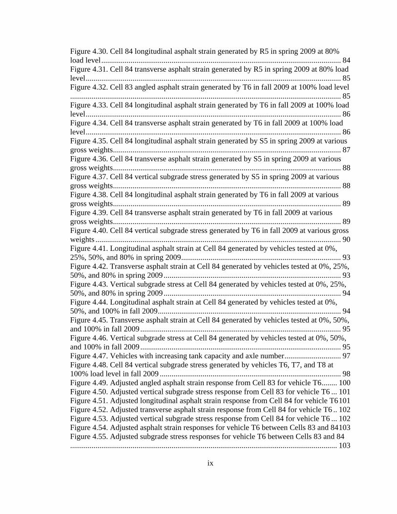
each. Figure 2.6 shows the cross-sectional detail of the instrumentation and Figure 2.7

shows the sensor layout for Cells 83 and 84, respectively for the westbound lane. Similar

layout was replicated for the eastbound lane with the exception of LVDTs.

The strain gage array was separated into three sets to capture critical pavement responses

under the various types of axle configurations found on agricultural vehicles. This sensor

arrangement allowed for redundancy in the measurements. Emphasis was made on the

outer wheel path of the vehicles; hence the first set of strain gages was installed one foot

from the pavement edge. The next two sets were spaced two feet apart, transverse to the

direction of traffic. For each strain gage set, a corresponding earth pressure cell was

installed along the same transverse offset. Each strain gage set consisted of three

orientations, which were placed longitudinally, angled at 45º, and transversely to the

direction of traffic. These three strain gages were installed two feet apart longitudinally.

LVDTs were installed with two feet spacing longitudinally and three feet from the

Megadec-TCS System

NI System

10

pavement edge. Both the thermocouple and TDR were installed at center lane with four

feet apart longitudinally.

Because of the wide variety of sensor orientations and positions, an appropriate sensor

labeling system was adopted. Longitudinal, angled, and transverse strain gages were

denoted as LE, AE, and TE, respectively. All earth pressure cells were denoted as PG.

Each sensor set corresponds to the transverse offset from the pavement edge; therefore

numeric labels were used to denote these sensor sets. The westbound lane sensor sets

were numbered 4, 5, and 6 with set 4 being closest to the pavement edge and set 6 being

closest to center lane. On the eastbound lane, sensor sets were numbered 1, 2, and 3 with

1 being closest to the pavement edge and 3 being closest to center lane. Final designation

for those sensors had the following form: [Cell #]-[Sensor Type]-[Set #]. For example,

the angled strain gage closest to the pavement edge of Cell 83 was designated as 83AE4.

Instrumentation of LVDTs on the westbound lanes of the flexible sections were placed

three feet from the pavement edge. The purpose of the LVDTs was to measure

displacements in the base layer in three directions; two horizontally in the longitudinal

and transverse directions and one vertically. These sensors were denoted as AL1, AH2,

and AV3, respectively. Because LVDTs were installed at one transverse offset, the

numeric notations from the above sensors do not apply. For example, the vertically

oriented LVDT of Cell 84 was denoted as 84AV3. Figure 2.8 shows the sensor

designations on the sensor layout for westbound lanes of the flexible pavement sections

Cells 83 and 84.

11

Traffic Direction

3.5"

HM

A8.

0" A

ggre

gate

Bas

eSu

bgra

de S

oil

2' 2' 2' 2'8' 10'

4"

Strain GaugeEarth Pressure CellLVDT

(a)

Traffic Direction

5.5"

HM

A9.

0" A

ggre

gate

Bas

eS

ubgr

ade

Soi

l

Strain GaugeEarth Pressure CellLVDT

4.5"

2' 2' 2' 2' 2'13'

(b)

Figure 2.6. Cross-sectional instrumentation detail of (a) Cell 83 (b) Cell 84

12

-20

-15

-10

-5

0

5

10

15

20

-10 -8 -6 -4 -2 0 2 4 6 8 10

Transverse Offset [ft]

Long

itudi

nal O

ffset

[ft]

Strain GaugeEarth Pressure CellLVDTThermocoupleTDR

Traf

fic D

irect

ion

Cen

ter L

ine

Pav

emen

t Edg

e to

6 ft

Agg

rega

te

Sho

ulde

r

Inner Wheelpath Outer Wheelpath

(a)

-20

-15

-10

-5

0

5

10

15

20

-10 -8 -6 -4 -2 0 2 4 6 8 10

Transverse Offset [ft]

Long

itudi

nal O

ffset

[ft]

Strain GaugeEarth Pressure CellLVDTThermocoupleTDR

Traf

fic D

irect

ion

Cen

ter L

ine

Pav

emen

t Edg

e to

6 ft

Pav

ed

Sho

ulde

r

Inner Wheelpath Outer Wheelpath

(b) Figure 2.7. Sensor layout for flexible pavement sections (a) Cell 83 (b) Cell 84

13

(a) (b)

Figure 2.8. Flexible pavement sections sensor designations for westbound lanes of

(a) Cell 83 (b) Cell 84

As mentioned previously, the data acquisition systems employed in this study to collect

pavement response data were the Megadec-TCS system for strain gages and earth

pressure cells and the NI system for the LVDTs as shown in Figure 2.5. These systems

collect response measurements at a rate of 1,200 data points per second (1,200 Hz) and

each vehicle pass typically have a collection time of fifteen to eighteen seconds. In total

there are approximately 18,000 to 22,000 data points per sensor. These data points

provide a response waveform of the asphalt strains, subgrade stresses, and base

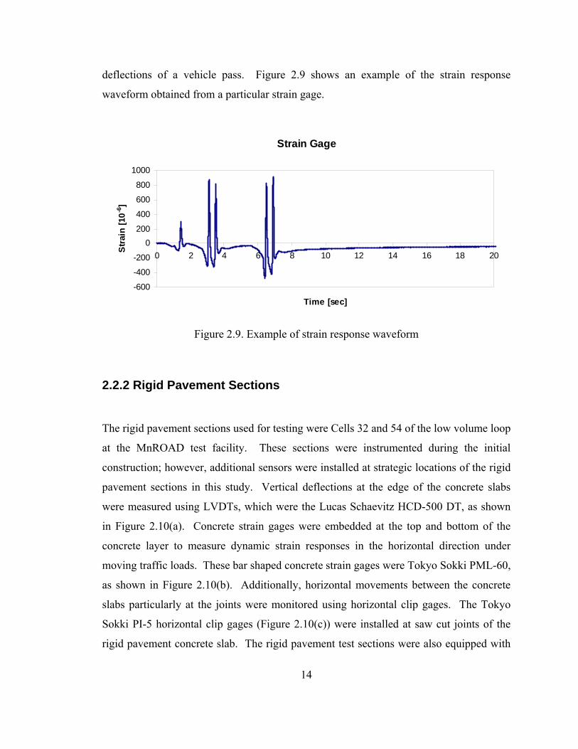
14

deflections of a vehicle pass. Figure 2.9 shows an example of the strain response

waveform obtained from a particular strain gage.

Strain Gage

-600

-400

-200

0200

400

600

800

1000

0 2 4 6 8 10 12 14 16 18 20

Time [sec]

Str

ain

[10-6

]

Figure 2.9. Example of strain response waveform

2.2.2 Rigid Pavement Sections

The rigid pavement sections used for testing were Cells 32 and 54 of the low volume loop

at the MnROAD test facility. These sections were instrumented during the initial

construction; however, additional sensors were installed at strategic locations of the rigid

pavement sections in this study. Vertical deflections at the edge of the concrete slabs

were measured using LVDTs, which were the Lucas Schaevitz HCD-500 DT, as shown

in Figure 2.10(a). Concrete strain gages were embedded at the top and bottom of the

concrete layer to measure dynamic strain responses in the horizontal direction under

moving traffic loads. These bar shaped concrete strain gages were Tokyo Sokki PML-60,

as shown in Figure 2.10(b). Additionally, horizontal movements between the concrete

slabs particularly at the joints were monitored using horizontal clip gages. The Tokyo

Sokki PI-5 horizontal clip gages (Figure 2.10(c)) were installed at saw cut joints of the

rigid pavement concrete slab. The rigid pavement test sections were also equipped with

15

thermocouple trees to measure pavement temperature at various depths of the concrete

and base layers. The same data acquisition systems that were used at the flexible

pavement section were also used at the rigid pavement section. The NI system and the

Megadec-TCS system collected LVDT measurements and strain measurements,

respectively.

(a) (b)

(c)

Figure 2.10. Rigid pavement instrumentation (a) Linear variable differential transformer

(LVDT) (b) Bar shape strain gage (c) Horizontal clip gage

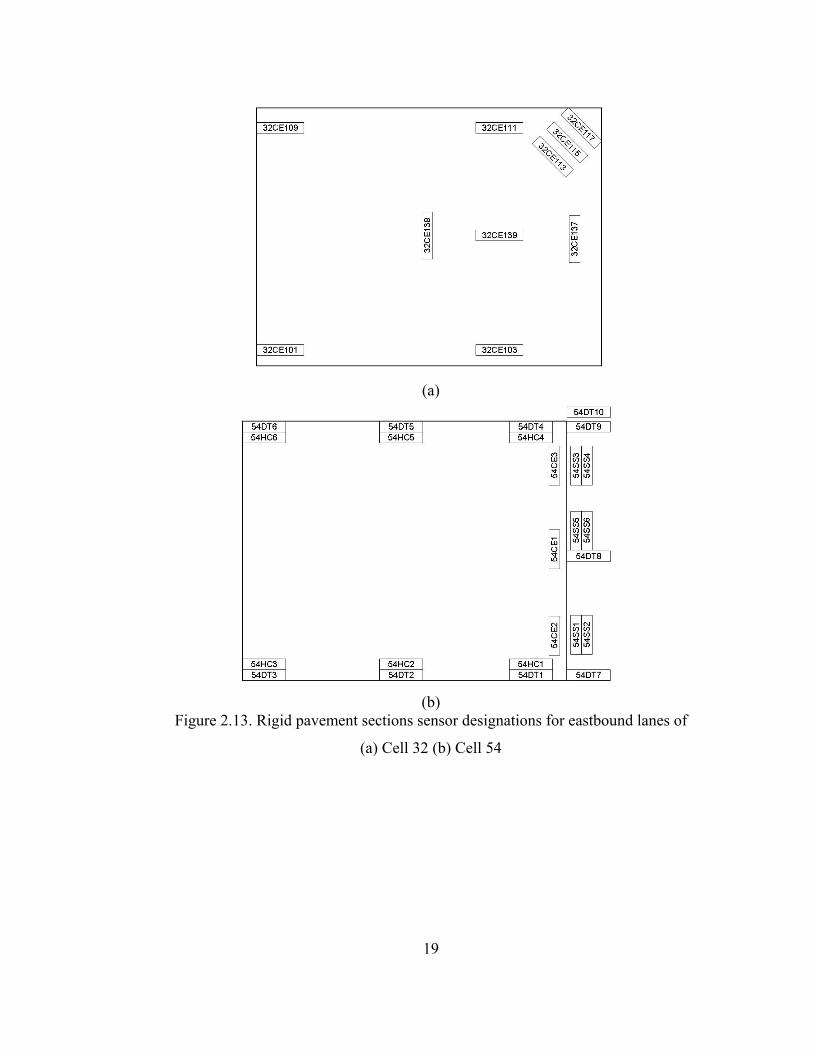
The tests performed at the rigid pavement sections were conducted in the eastbound

lanes. It should be noted that instrumentation of the rigid pavement sections (Cells 32

and 54) are different from one another. At Cell 32, only the embedded bar shape strain

gages were installed in addition to thermocouples. A total of ten strain gages were

installed at Cell 32: five of which measure strain transverse to the direction of traffic, two

in the longitudinal direction, and three strain gages were angled at 45º. These strain

gages were installed at the near surface to measure strains at the top of the concrete layer.

16

Cell 54 consisted of a wider array of sensors compared to Cell 32. Cell 54 was

instrumented with four vertical LVDTs at the slab edge, six horizontal LVDTs and six

horizontal clip gages in between joints, three strain gages embedded at the edge of the

concrete slab, and six more strain gages at the edge of the concrete slab. Thermocouples

were also installed in Cell 54 at varying depths. Figure 2.11 shows the cross-sectional

detail of the instrumentation and Figure 2.12 shows the sensor layout for Cells 32 and 54

for the eastbound lane.

Similar to the flexible pavement sections, each of the installed sensors was given a

unique sensor label. Sensors were labeled according to their cell location, sensor type,

and number as such: [Cell #]-[Sensor Type]-[Sensor #]. Strain gages were denoted as CE

and SS whereas LVDTs and clip gages were denoted as DT and HC, respectively. For

Cell 54, several sensors were overlapped as seen in the layout view (Figure 2.12(b)). It

should be noted that the horizontal LVDTs are 0.5 in. above the horizontal clip gages (i.e.

LVDTs 54DT1 to 54DT6 are placed above clip gages 54HC1 to 54HC6, respectively).

Strain gages 54SS1 and 54SS3 are located 6 in. above strain gages 54SS2 and 54SS4,

respectively. Sensor 54SS5 is located 5.5 in. above 54SS6. Unfortunately, these

designations do not provide information regarding the sensor orientations. Figure 2.13

shows the sensor designations for both Cells 32 and 54.

17

5.0"

PC

CS

ubgr

ade

Soi

l1.

0" C

lass

-1f

6.0"

Cla

ss-1

c

5' 3' 1' 1'

~0.2"

Traffic Direction

Strain Gauge

(a)

Traffic Direction

7.5"

PC

C12

.0"

Cla

ss-6

Sub

grad

e So

il

Strain Gauge

Horizontal LVDTVertical LVDT

Clip Gauge

4.25' 3.25'

7.5' 7.3' 0.3'

~0.4"

~0.1"

~0.5"

~0.5" 3.0"

3.5"

(b)

Figure 2.11. Cross-sectional instrumentation detail of (a) Cell 32 (b) Cell 54

18

-2

0

2

4

6

8

10

12

-2 0 2 4 6 8 10 12 14Transverse Offset [ft]

Long

itudi

nal O

ffset

[ft]

Cen

ter L

ine/

Lo

ngitu

dina

l Joi

nt

Outer Wheelpath

Pav

emen

t Edg

e to

10

ft A

ggre

gate

S

houl

der

Transverse Joint

Transverse Joint

Traf

fic D

irect

ion

Strain Gauge

(a)

-2

0

2

4

6

8

10

12

14

16

18

-2 0 2 4 6 8 10 12 14Transverse Offset [ft]

Long

itudi

nal O

ffset

[ft]

Cen

ter L

ine/

Lo

ngitu

dina

l Joi

nt

Outer Wheelpath

Pav

emen

t Edg

e to

10

ft A

ggre

gate

Transverse Joint

Transverse Joint

Traf

fic D

irect

ion

Strain Gauge

Horizontal LVDTVertical LVDT

`

Clip Gauge

(b) Figure 2.12. Sensor layout for rigid pavement sections (a) Cell 32 (b) Cell 54

19

(a)

(b)

Figure 2.13. Rigid pavement sections sensor designations for eastbound lanes of

(a) Cell 32 (b) Cell 54

20

2.3 Field Testing

A significant portion of heavy agricultural traffic occurs in spring and fall seasons.

Pavement behavior and corresponding damage accumulation during these seasons can be

quite different. Temperature and moisture variations induce changes in the material

properties of the pavement structure. To account for these effects, field testing was

conducted twice a year, in March and August.

Tests conducted in March aimed to evaluate pavement behavior under spring conditions.

During the spring season, the frozen layers within the pavement structure begin to thaw,

saturating the layers with trapped water. This saturation creates a pore pressure and

cohesionless condition mainly in the base and subgrade layers, resulting in a generally

weakened state of the pavement structure.

In the fall season, a relatively high volume of heavily loaded agricultural vehicles can be

expected. The asphalt layer is also less stiff than in spring, and more prevalent damage to

the asphalt layer can be expected under similar loading conditions. While September is

the month most representative of typical fall conditions, testing was conducted in August

due to unavailability of agricultural vehicles and operators supplied by the industry. In

this document, tests conducted in August were referred to as fall season tests. Since

August is one of the hottest months of the year in Minnesota, the results obtained for

August may be somewhat conservative for fall conditions.

Large amounts of information were obtained during testing, most importantly strain,

stress, and deflection data of the pavement through the heavily instrumented pavement

sections. Pavement response data were collected using two data acquisition systems set

up by MnROAD personnel. The Megadec-TCS system controlled and collected data

from the strain gages and earth pressure cells whereas the NI system was dedicated only

to the LVDTs. Every successful vehicle pass corresponded to one Megadec-TCS file and

one NI file. Each of these files had unique filenames and was recorded in the test

21

program data logs. In addition, information regarding the tested vehicles was also

obtained such as vehicle axle configurations, wheel dimensions, and wheel weights at

different load levels. It was also determined that traffic wander is a crucial piece of

information in this study that was measured for every vehicle pass. Since agricultural

vehicles have complex tire patterns, the footprint of each vehicle was recorded at various

load levels. This was made possible with the use of the Tekscan device which is capable

of measuring tire contact area and contact stress.

Field testing was conducted in 2008, 2009, and 2010. For each round of testing, a test

program was developed specifically for the availability of vehicles and manpower. A

total of twelve agricultural vehicles were tested throughout the duration of this study. An

additional two typical five-axle semi tractor-trailer were included in the test to be used as

reference vehicles. These semis have a gross vehicle weight of 80 kip and 102 kip

labeled as Mn80 and Mn102, respectively. Due to the large number of vehicles, each

vehicle was given a unique vehicle ID to simplify the identification process. A list of

vehicles that were tested in this study is summarized in Table 2.3. Images of all tested

vehicles are shown in Figure 2.14.

22

Table 2.3. List of vehicles tested

Vehicle ID Type Vehicle Make Size # of Axles

Spring08

Fall08

Spring09

Fall09

Spring10

Fall10

S4 Truck Homemade 4,400 gal 3 ● ● S5 Truck Homemade 4,400 gal 3 ● ● S3 Terragator AGCO Terragator 8204 1,800 gal 2 ● R4 Terragator AGCO Terragator 9203 2,400 gal 2 ● ● R5 Terragator AGCO Terragator 8144 2,300 gal 2 ● ● R6 Terragator AGCO Terragator 3104 4,200 gal 2 ●

T1 Tanker John Deere 8430 w/ Houle tank 6,000 gal 4 ●

T2 Tanker M. Ferguson 8470 w/ Husky tank 4,000 gal 4 ●

Tanker John Deere 8430 w/ Husky tank 6,000 gal 4 ● ●

Tanker John Deere 8230 w/ Husky tank 6,000 gal 4 ● ● ● T6

Tanker New Holland TG245 w/ Husky tank 6,000 gal 4 ●

Tanker Case IH 245 w/ Houle tank 7,300 gal 5 ● Tanker Case IH 335 w/ Houle tank 7,300 gal 5 ● T7 Tanker Case IH 275 w/ Houle tank 7,300 gal 5 ● Tanker Case IH 485 w/ Houle tank 9,500 gal 6 ● T8 Tanker Case IH 335 w/ Houle tank 9,500 gal 6 ● ●

G1 Grain Cart Case IH 9330 w/ Parker 938 cart 1,000 bushels 3 ●

Mn80 Semi Truck Navistar NA 5 ● ● ● ● ● ● Mn102 Semi Truck Mack NA 5 ● ● ● ●

23

S4 (Homemade 4,400 gal – radial tires) S5 (Homemade 4,400 gal – flotation tires)

S3 (AGCO Terragator 8204) R4 (AGCO Terragator 9203)

R5 (AGCO Terragator 8144) R6 (AGCO Terragator 3104)

T1 (John Deere 8430, 6,000 gal) T2 (M. Ferguson 8470, 4,000 gal)

24

T6 (John Deere 8230, 6,000 gal) T7 (Case IH 335, 7,300 gal)

T8 (Case IH 335, 9,500 gal) G1 (Case IH 9330, 1,000 bushels)

Mn80 (Navistar 80-kip) Mn102 (Mack 102-kip)

Figure 2.14. Images of tested vehicles

25

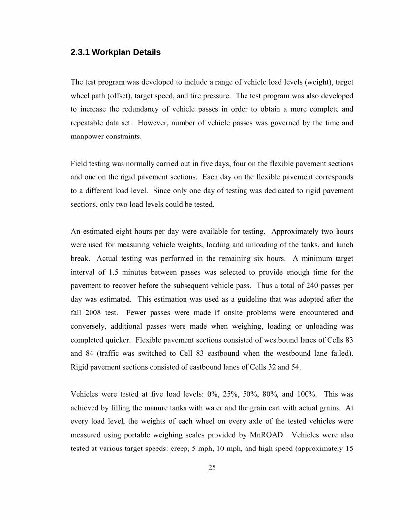
2.3.1 Workplan Details

The test program was developed to include a range of vehicle load levels (weight), target

wheel path (offset), target speed, and tire pressure. The test program was also developed

to increase the redundancy of vehicle passes in order to obtain a more complete and

repeatable data set. However, number of vehicle passes was governed by the time and

manpower constraints.

Field testing was normally carried out in five days, four on the flexible pavement sections

and one on the rigid pavement sections. Each day on the flexible pavement corresponds

to a different load level. Since only one day of testing was dedicated to rigid pavement

sections, only two load levels could be tested.

An estimated eight hours per day were available for testing. Approximately two hours

were used for measuring vehicle weights, loading and unloading of the tanks, and lunch

break. Actual testing was performed in the remaining six hours. A minimum target

interval of 1.5 minutes between passes was selected to provide enough time for the

pavement to recover before the subsequent vehicle pass. Thus a total of 240 passes per

day was estimated. This estimation was used as a guideline that was adopted after the

fall 2008 test. Fewer passes were made if onsite problems were encountered and

conversely, additional passes were made when weighing, loading or unloading was

completed quicker. Flexible pavement sections consisted of westbound lanes of Cells 83

and 84 (traffic was switched to Cell 83 eastbound when the westbound lane failed).

Rigid pavement sections consisted of eastbound lanes of Cells 32 and 54.

Vehicles were tested at five load levels: 0%, 25%, 50%, 80%, and 100%. This was

achieved by filling the manure tanks with water and the grain cart with actual grains. At

every load level, the weights of each wheel on every axle of the tested vehicles were

measured using portable weighing scales provided by MnROAD. Vehicles were also

tested at various target speeds: creep, 5 mph, 10 mph, and high speed (approximately 15

26

to 25 mph). Testing at operating speeds was not possible due to insufficient distance at

the end of the test sections for the vehicles to slow down.

One of the objectives of the test program was to evaluate the effect of vehicle traffic

wander on pavement responses. The pavement edges were marked as the fog line and

vehicles were directed to travel with the target offsets of 0 in., 12 in., or 24 in. from the

fog line. To determine the actual wheel paths, length scales were painted onto the

pavement surfaces in fall 2008 which were later replaced by permanent steel scales.

Videos of the vehicle passes were recorded using a video camera.

As the tests were conducted, the data acquisition operator recorded the actual time of

each vehicle pass and the corresponding data files which were saved by two of the data

acquisition systems. This step was necessary to remove any false triggering of the

acquisition system and to make sure that the acquired data files corresponded correctly to

the pass information. An example of the test program is shown in Appendix A.

2.3.2 Vehicle Measurements

The test program required vehicles to be tested at varying load levels. For each load

level, measurements of the all vehicle weights were obtained using portable scales.

Portable scales were placed in front of each of the vehicles’ wheels and the vehicle was

carefully driven to place each wheel on top of the scales. It was ensured that the entire

vehicle was leveled and no weight bias occurred between axles and between wheels.

Figure 2.15 shows an example obtaining weight measurements using the portable scales.

Additionally, vehicle axle configurations, wheel spacing, and wheel widths were

measured for all tested vehicles. Appendix B contains the vehicle axle weights and

dimensions.

27

Figure 2.15. Weighing vehicles using portable scales

2.3.3 Traffic Wander Measurements

As already discussed, the test program required the vehicles to travel at various distances

(offsets) from the pavement edges. These offsets were targeted at 0, 12, and 24 in. from

the pavement edges and were based on the center of the most rear axle for every vehicle

to maintain consistency. Although vehicle operators were often precise with their

steering control to achieve the target offsets, it was still important to determine the

vehicles’ actual position. To achieve this objective, length scales were installed and

vehicle positions were recorded during each pass.

Initially, scales were painted onto the pavement surface using scaled pavement stencils,

but the paint quickly faded with increasing number of traffic. Therefore, steel scales with

1 in. teeth spaced 1 in. apart were fabricated and installed onto the pavement surface at

each of the test sections (i.e. Cells 83, 84, 32, and 54) as a more permanent solution.

Figure 2.16 shows the initial painted scale and the more permanent steel scale installed at

Cell 84 of the flexible pavement section. The scales were installed as close as possible to

the sensor locations, but not too close as it may affect pavement response measurements.

Video cameras were placed at each cell of the test sections and configured to produce the

28

optimal view of the scale. A Sony and a Panasonic video camera were used in this

measurement. Figure 2.17 shows the video camera used for this measurement and an

example of a vehicle pass as it drives over the painted scale.

Figure 2.16. Permanent steel scale and painted scale at Cell 84

(a) (b)

Figure 2.17. Traffic wander measurements (a) using the Panasonic video camera

(b) for a vehicle pass

Video recordings of each vehicle pass were taken as the vehicle travels across the scales.

Camera operators began recording the videos as the vehicle approaches the scale and

called out the test number and vehicle ID in the video recording. This ensured that the

videos can be properly matched with the corresponding data files and pass information.

The videos were later viewed and evaluated individually to determine the actual vehicle

offsets.

Steel scale

Painted scale

29

2.4 Tekscan

As mentioned previously, heavy agricultural vehicles are equipped with tires that have

complex load distributions in terms of tire-soil interaction. Characteristics of these tires

depend on the construction whether they are radial ply or bias ply. In addition, there are

also flotation tires that are now increasingly common in the agricultural industry.

Flotation tires are designed to have a much wider footprint and lower inflation pressure

compared to conventional tires. These tires have tread patterns (tire lugs) that allow the

vehicle to maneuver safely and efficiently as well as provide the vehicle with adequate

support over soft materials. In the agricultural industry, a larger footprint and lower

inflation pressure is sought because it helps to reduce rutting and compaction of the soil

in the field.

In this study, measurements of tire footprint and vertical contact stress were obtained

using a device called Tekscan. This device consists of four sensorial mats (model

5400N) and four data handles (Evolution Handles) with attached USB cables, as shown

in Figure 2.18. Each of the sensorial mats is approximately 24 in. by 36 in. with a

sensing area of 22.76 in. by 34.80 in. The mats were placed according to the 5400NQ

sensor map as per Tekscan Inc. recommendation, shown in Figure 2.19. This setup

requires four 5400N sensorial mats to be positioned in a two by two arrangement. Using

the 5400NQ setup, the sensing area is 45.51 in. by 69.61 in. Each sensorial mat was

connected to one Evolution Handle as shown in Figure 2.19 and connected to the USB

ports of the computer. Data was collected using the I-Scan version 5.90 software.

30

(a) (b)

Figure 2.18. Tekscan hardware components (a) 5400N sensor mats (b) Evolution Handle

The Tekscan setup and testing involved the following steps [8]:

1. The 5400N sensorial mats and Evolution Handles were placed as shown in Figure

2.19. Sensorial mats were placed on top of a flat steel sheet to protect it from the

underlying rough pavement surface. These mats were also protected with plastic

sheets to prevent damage from the vehicle pass.

2. Handles A and B were positioned from left to right along the top of the array

while handles C and D were positioned from left to right along the bottom of the

array.

3. Sensorial mats A and D were placed with the words “This Side Up” facing right

side up while sensorial mats B and C were positioned with the words “This Side

Up” facing down.

4. All sensorial mats were clamped to the corresponding handles according to their

positions.

5. The handles were connected to a computer and checks were performed to ensure

that all connections were secured and complete.

6. The Sensor OK LED must be lit green to indicate that sensorial mats were

correctly inserted to the handles. The Power LED must be lit green to indicate

handles are receiving power and has been initialized by the computer.

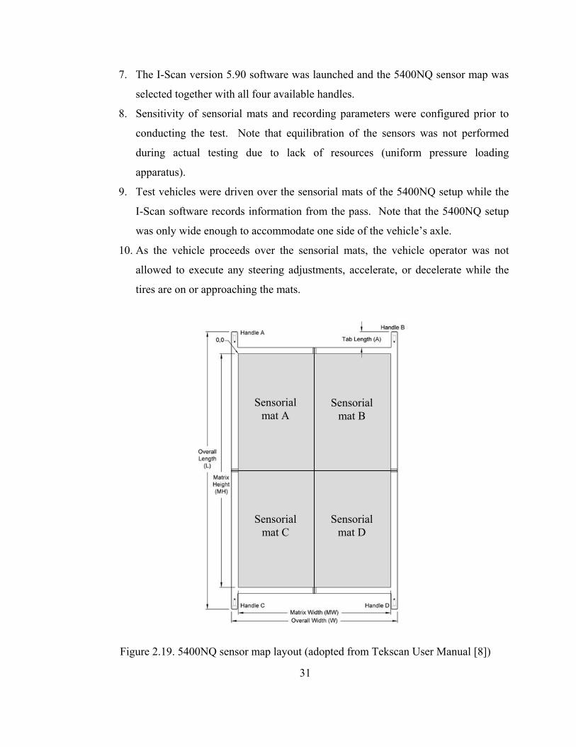
31

7. The I-Scan version 5.90 software was launched and the 5400NQ sensor map was

selected together with all four available handles.

8. Sensitivity of sensorial mats and recording parameters were configured prior to

conducting the test. Note that equilibration of the sensors was not performed

during actual testing due to lack of resources (uniform pressure loading

apparatus).

9. Test vehicles were driven over the sensorial mats of the 5400NQ setup while the

I-Scan software records information from the pass. Note that the 5400NQ setup

was only wide enough to accommodate one side of the vehicle’s axle.

10. As the vehicle proceeds over the sensorial mats, the vehicle operator was not

allowed to execute any steering adjustments, accelerate, or decelerate while the

tires are on or approaching the mats.

Figure 2.19. 5400NQ sensor map layout (adopted from Tekscan User Manual [8])

Sensorial mat A

Sensorial mat B

Sensorial mat C

Sensorial mat D

32

Testing was limited to the availability of the vehicles but Tekscan measurements were

obtained for almost all the vehicles tested in the farm loop, as shown in Table 2.4.

Table 2.4. Tekscan tested vehicle list

Test Date Vehicles Load Levels [%] March 17 2008 S4, S5, T1 0, 50, 80 March 26 2008 S3, T2, T6, Mn80 0, 50, 80 August 28 2008 R4, T7 0, 25, 80 August 29 2008 T8 0, 25, 80

2.5 Test Overview

The following experiments were conducted during each round of testing:

• Spring 2008 (March 17 to 19 and 24 to 26)

o Tested seven vehicles; S3, S4, S5, T1, T2, T6, and Mn80.

o Load levels: 0%, 25%, 50%, and 80%.

o Vehicle speeds: creep, 5 mph, and 10 mph.

o Vehicle offsets: 0 and 12 in.

o Tire pressure for vehicle T1: 33 and 42 psi.

o No measurements of traffic wander.

• Fall 2008 (August 26 to 29)

o Tested five vehicles; R4, T6, T7, T8, and Mn80.

o Load levels: 0%, 25%, 50%, and 80%.

o Vehicle speeds: creep, 5 mph, and 10 mph.

o Vehicle offsets: 0 and 12 in.

o Excluded need to change tire pressure. All vehicles have tire pressures

which they normally operate by.

o Scales were painted onto the pavement surface and videos of vehicle

wheel path were recorded to estimate traffic wander.

33

• Spring 2009 (March 16 to 20)

o Tested nine vehicles; S4, S5, R4, R5, T6, T7, T8, Mn80, and Mn102.

o Load levels: 0%, 25%, 50%, and 80%.

o Vehicle speeds: 5 mph, 10 mph, and high speed (15 to 25 mph). Excluded

creep speed.

o Vehicle offsets: 0 and 12 in.

o Permanent steel scales were installed onto the pavement to assist in traffic

wander estimation.

o Failure occurred at Cell 83 westbound during test at 50% load level.

Failure was propagated at 80% load level.

o Failed section was patched for upcoming tests.

• Fall 2009 (August 24 to 28)

o Tested six vehicles; R5, T6, T7, T8, Mn80, and Mn102.

o Load levels: 0%, 50%, and 100%. Excluded 25% load level.

o Vehicle speeds: 5 mph, 10 mph, and high speed.

o Vehicle offsets: 0, 12, and 24 in. 24 in offsets were included due to

recommendations from the technical committee.

o Failure at patched section of Cell 83 westbound during test at 0% load

level on the first day. Testing was switched to Cell 83 eastbound.

o Failure at Cell 83 eastbound during test at 50% load level on the second

day. Testing was switched back to Cell 83 westbound with steel sheets

placed over failure section.

o Failure propagated at Cell 83 westbound during test at 100% load level.

o Failure sections on both east and westbound lanes of Cell 83 were not

repaired for consecutive tests. Instead, steel sheets which were placed will

remain for future tests. Additional steel sheets were placed at propagated

failure sections.

34

• Spring 2010 (March 15 to 18)

o Tested four vehicles; R6, T6, Mn80, and Mn102.

o Load levels: 0%, 50%, and 100%.

o Vehicle speeds: 10 mph and high speed. 5 mph vehicle speeds were

excluded.

o Vehicle offsets: 0, 12, and 24 in.

o Existing failure on Cell 83 westbound continued to propagate.

o Both westbound and eastbound lanes of Cell 83 were dismissed from

future tests.

• Fall 2010 (August 18 to 19)

o Tested four vehicles; T6, G1, Mn80, and Mn102.

o Load levels: 0% and 100%. Other load levels were excluded due to

availability of vehicle G1.

o Vehicle speeds: 10mph only. Other vehicles speeds were excluded from

the test.

o Vehicles offsets: 0, 12, and 24 in.

Table 2.5 summarizes the number of vehicle passes made on the flexible (AC sections)

and rigid (PCC sections) pavement sections for each round of testing.

Table 2.5. Overview of previous test

Vehicle Passes Test Season Test Dates AC PCC

Spring 2008 March 17 – 19 & 24 – 26 400 48 Fall 2008 August 26 – 29 282 72

Spring 2009 March 16 – 20 960 170 Fall 2009 August 24 – 28 782 360

Spring 2010 March 15 – 18 776 344 Fall 2010 August 18 – 19 426 204

Total 3,626 1,198

35

2.6 Pavement Distress Monitoring

After each round of testing, distress surveys were conducted. Initial signs of pavement

distress were observed on third day of testing during spring 2009 (18 March 2009). At

Cell 83 westbound lane, a longitudinal crack developed approximately 12 in. away from

the pavement edge toward the center line. The condition of the pavement surrounding

the longitudinal crack further deteriorated with increasing number of vehicle passes. At

the end of the following day of testing (19 March 2009), the pavement section had

completely failed in extreme rutting. The total length of the rut was approximately 31.5

ft. at just 14.5 ft. away from the closest sensor location. Figure 2.20 and Figure 2.21

show the initial longitudinal crack and the subsequent rutting failure of Cell 83

westbound lane in spring 2009.

Figure 2.20. Failure at Cell 83 westbound lane on 18 March 2009

Figure 2.21. Failure at Cell 83 westbound lane on 19 March 2009

36

The failed section of Cell 83 westbound lane was repaired and patched in preparation for

fall 2009 test. On 24 August 2009 which was the first day of testing in fall 2009, the

patched area experienced slippage cracks shown in Figure 2.22. This failure was due to

insufficient bonding between the wearing and binder courses of the asphalt layer. Testing

was shifted to Cell 83 eastbound lane where it unexpectedly failed on the 25 August

2009. Before testing was shifted back to Cell 83 westbound lane, the previous slippage

cracks were overlaid with ¾ in. steel plates in an attempt to slow down the pavement

deterioration as number of vehicle passes and load levels increase. However,

deterioration of that section was imminent and rutting at the pavement edge continued to

propagate until the last day of fall 2009 test (27 August 2009). A forensic study was

conducted on the failure site and a report prepared by the Minnesota Department of

Transportation suggested that the clay borrow layer was the cause for the pavement

failure [9].

Figure 2.22. Slippage cracks at Cell 83 westbound lane on 24 August 2009

37

Chapter 3 Data Processing and Archiving

Since a large amount of information was collected in this study, it was necessary to

develop procedures for efficient processing and archiving of the collected data. Raw data

acquired directly from the field tests needed to be summarized in a usable format for

analysis. The raw data includes video files containing vehicle traffic wander, pavement

response data containing time history of asphalt strains, subgrade stresses, and base

deflections generated by the vehicles, and Tekscan measurements containing contact area

and contact stress information of the tested vehicles. This chapter contains information

pertaining to initial processing of this information and organization into summary tables.

This is followed by a description of the data organization and archiving that was

developed to provide convenient accessibility to the data for subsequent analysis.

3.1 Determining Vehicle Traffic Wander

Test vehicles were directed to travel at lateral distances of 0, 12, and 24 in. away from the

pavement edge. The actual traffic wander could be significantly different from the target

offsets. To provide the necessary precision for interpreting the data the actual vehicle

offsets were measured. Scales were installed on the pavement surface at both cells of

both test sections and video cameras were used to record the vehicle pass as it travels

across the scales. As the vehicle approaches the scales, the camera operator mentioned

the test number and vehicle ID as per the test program so that the videos could be

matched with the corresponding data file and pass information.

The video files were stored in an external hard disk. Depending on the video camera

manufacturer, the video files were saved in different file extensions. Videos recorded

using a Panasonic camera have extensions “.mod” while files ending with extension

“.moi” were ignored. Videos from the Sony camera have file extensions “.mts”. After

transferring the video files, they were then played in a preferred media player. During

38

this step, identification of the video file corresponding to the test number and vehicle ID

was performed. Once the video file was matched to its corresponding pass information, it

was renamed according to the following format: [Load Level]-[Pass #]-[Target Speed]-

[Vehicle ID]-[Cell #]. For example, a raw video file named MOV006.mod of Cell 83,

Day 1 (08-24-09) was found to correspond to test number two for vehicle R5. Hence the

file was renamed to 0%-1-5-R5-C83. The next step involved determining the actual

offset of the vehicles’ wheel path as described below:

1. For each vehicle pass, video files were played in a preferred media player. The

video was paused when the last axle of the vehicle was directly on top of the steel

scale (see Figure 3.1).

2. The red strip on the steel scale placed on the outer edge of the fog line (pavement

edge) was designated as the origin. Wheel paths toward the centerline of the

pavement were considered to be positive while toward the shoulder were

considered to be negative.

3. The wheel edge offset was obtained by counting the number of teeth and gaps

(each 1 in. wide) from the origin to the last visible tooth or gap at the edge of the

wheel of the vehicle’s last axle (see Figure 3.2).

4. Wheel center offset was obtained by simply adding the wheel edge offset to half

the tire width of the last axle.

Figure 3.3 shows an example of obtaining the wheel edge and center offsets for a generic

11 in. wide tire.

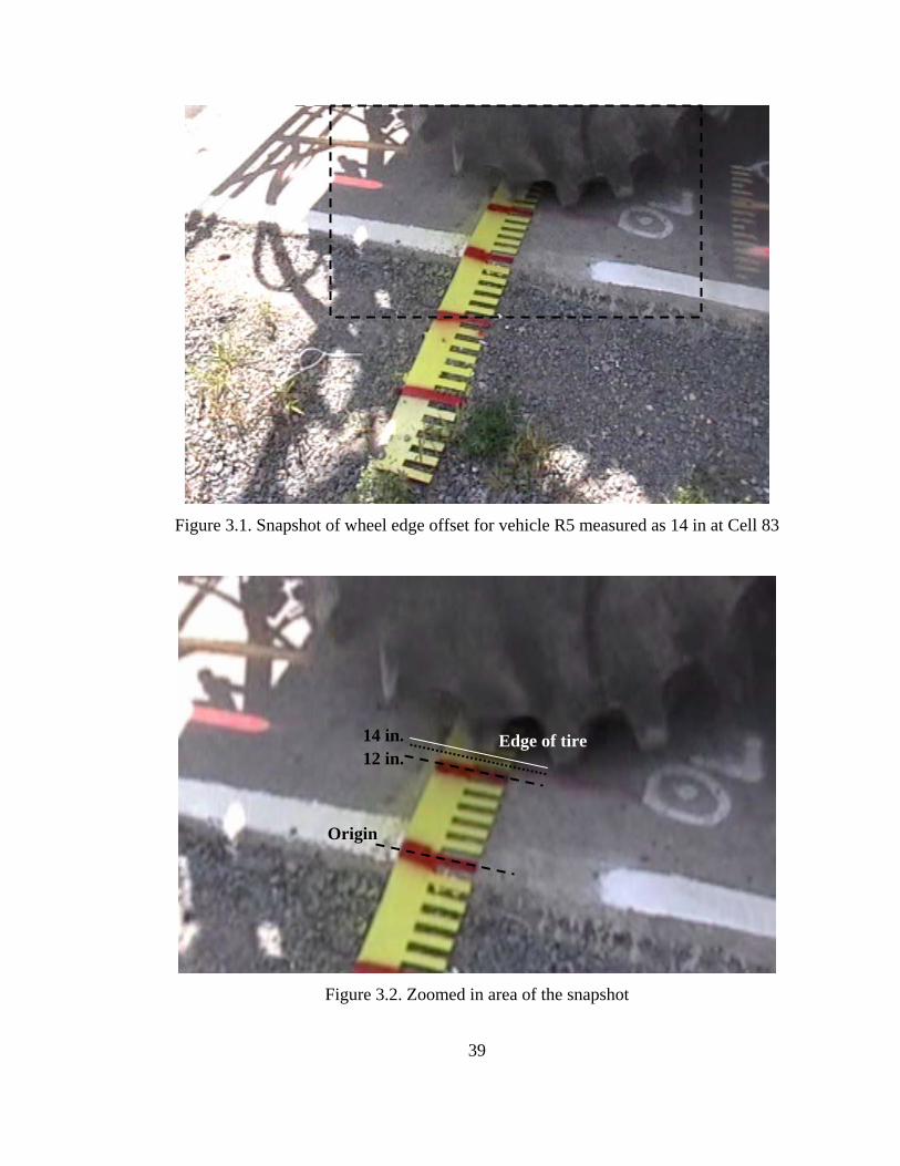
39

Figure 3.1. Snapshot of wheel edge offset for vehicle R5 measured as 14 in at Cell 83

Figure 3.2. Zoomed in area of the snapshot

Origin

12 in. 14 in. Edge of tire

40

Figure 3.3. Wheel edge and wheel center offsets for a generic 11 in. tire width

0

12

-12

6

-6

Wheel path 1

Wheel path 2 W

heelpath 3

Tire width: 11 in. Wheel Edge Offsets Wheel path 1: 3 Wheel path 2: 0 Wheel path 3: -6 Wheel Center Offsets Wheel path 1: 8.5 Wheel path 2: 5.5 Wheel path 3: -0.5

Toward centerline

Toward shoulder

Direction of traffic

41

3.2 Pavement Response Data

Several steps were required in analyzing the pavement response data. This includes the

strain and stress data files acquired through the Megadec-TCS acquisition system and the

LVDT data files acquired through the NI acquisition system. The process began with

determination of which sensors were properly functioning. Next, the Peak-Pick analysis

was performed on the data files to extract pertinent axle responses. The Peak-Pick output

files were then filtered and arranged in a format which was convenient to perform further

analysis.

3.2.1 Determining Sensor Status

Before any data analysis was performed, it was imperative to determine which of the

installed sensors were giving adequate responses. This check was done randomly for

each day of testing for at least five percent of the collected data. Example of responses

from a properly functioning strain gage, earth pressure cell, and LVDT are shown in

Figure 3.4 through Figure 3.6. Examples of responses from improperly functioning

sensors are shown in Figure 3.7 and Figure 3.8. Improperly functioning sensors were

determined when no trace of the response was found or the response was too noisy. A

list of the sensor status for each test season is included in Appendix C.

42

Strain Gage

-600

-400

-200

0200

400

600

800

1000

0 2 4 6 8 10 12 14 16 18 20

Time [sec]

Str

ain

[10-6

]

Figure 3.4. Response from a working strain gage

Earth Pressure Cell

-1

0

1

2

3

4

5

6

0 2 4 6 8 10 12 14 16 18 20

Time [sec]

Stre

ss [p

si]

Figure 3.5. Response from a working earth pressure cell

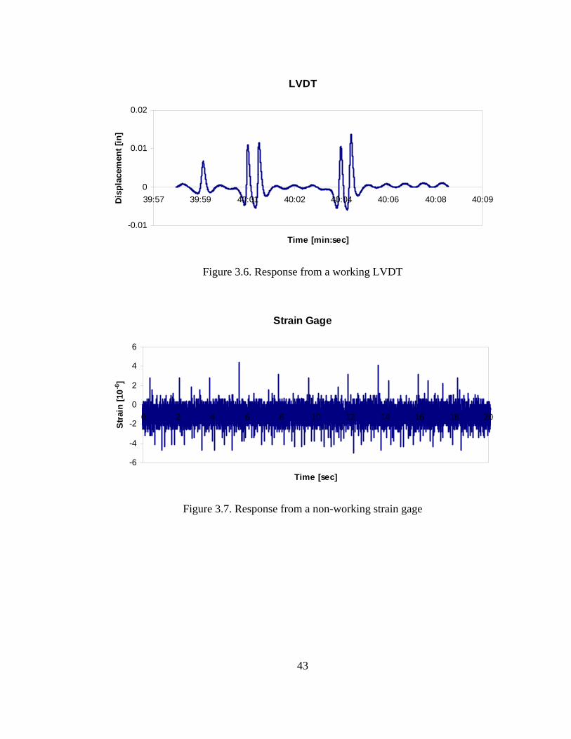
43

LVDT

-0.01

0

0.01

0.02

39:57 39:59 40:01 40:02 40:04 40:06 40:08 40:09

Time [min:sec]

Dis

plac

emen

t [in

]

Figure 3.6. Response from a working LVDT

Strain Gage

-6

-4

-2

0

2

4

6

0 2 4 6 8 10 12 14 16 18 20

Time [sec]

Stra

in [1

0-6]

Figure 3.7. Response from a non-working strain gage

44

LVDT

-0.02

-0.01

0

0.01

0.02

0.03

39:57 39:59 40:01 40:02 40:04 40:06 40:08 40:09

Time [min:sec]

Disp

lace

men

t [in

]

Figure 3.8. Response from a non-working LVDT

3.2.2 Peak-Pick Analysis

Due to the large amount of data points collected from one vehicle pass, a reduction

process was necessary to extract characteristic parameters for each response

measurement. To achieve this, the Peak-Pick program, developed for MnDOT by the

University of Minnesota, Department of Electrical and Computer Engineering, was

employed. For the purpose of this analysis, the Peak-Pick program was found to have

sufficient efficiency in locating maximum and minimum pavement responses from the

time history measurements generated by the vehicle pass. The following figure (Figure

3.9) shows the start-up screen for the Peak-Pick program and Table 3.1 gives a

description of each of the options available on the start-up screen. Further elaboration of

the information acquired for Table 3.1 and the Peak-Pick program can be found in the

Peak-Pick User Guide [10].

45

Figure 3.9. Peak-Pick start-up screen

46

Table 3.1. Peak-Pick program options

Option Description

Peak-Picking Modes

Seven modes are available for peak picking: Auto, semi-auto, manual, output correction, sensor label correction, output file split, and FWD. In this analysis, only the auto and manual modes were utilized.

Data Delimiter Data delimiter of the input files can be either space, comma, or tab separated. Data files used in this analysis are comma separated.

Baseline Selection Baseline selections can be either initial as well as final baseline only or include intermediate baseline values. This option was left at initial and baseline values only.

Data File Type Four options are available for data type: DOS1, DOS2, WINDOWS, and NI. Two of these selections were used in the analysis: WINDOWS and NI.

Results Plotting Feature

The plotting feature can be either turned on or off for storing the result plots for the response trace analyzed. This option was turned on to enable future checks if necessary.

Trigger Data Some data files contain a trigger column and should be identified before proceeding with the analysis.

Supplementary Time Stamp

Supplementary time stamps can be present in the form of IRIGB or CIRIG information. In this analysis, no time stamps were present.

Number of Vehicle Axles This program accommodates 2, 3, 4, 5, and 6 vehicle axles.

Sensor Designators

Sensor designators for the collected data files follow the MnROAD format.

Trace Quality Trace quality can be either good or bad. This option is especially useful as an additional filtering if the trace is bad.

Vehicle Type A feature which provides additional picking accuracy for a MnROAD type semi truck. The other option was selected for a non MnROAD semi truck.

Peak-Pick analysis was performed on all collected strain, stress, and deflection data. For

this analysis, there were two methods for the data to be analyzed: automatic and manual

modes. The automatic mode was the preferred approach. However, in some occasions

the peaks and troughs of the waveform were not successfully detected. For those cases

manual selection mode was required. In the manual selection, the Peak-Pick user

manually picked the peaks of the waveform. A description of the analysis process using

Peak-Pick, starting with the automatic selection and followed by manual selection mode

is shown below.

47

Automatic Selection for Strain and Stress Data Files (from Megadec-TCS System)

1. The number of axles on each vehicle tested was identified prior to running the

analysis.

2. Data files from the Megadec-TCS acquisition system for strain and stress

measurements were previewed to determine if a trigger column was present.

3. On the Peak-Pick start-up window, the following options were selected:

• Picking Mode: Auto

• Data Delimiter: Comma

• Baseline Selection: Initial and Final

• Data File Type: WINDOWS style

• Results Plotting Feature: On

• Trigger Data: Determined by previewing data files

• Supplementary Time Stamp: None

• Number of Vehicle Axles: Determined in step 1

• Sensor Designators: MnROAD

• Trace Quality: Good, unless a majority of response measurements are bad

• Vehicle Type: Other, unless the data file belongs to the MnROAD semi trucks

(i.e. Mn80 or Mn102)

4. The “Submit” button was clicked and input data files to be analyzed were

selected.

5. The directory in which the output file was to be written in was selected. The

output file directories were arranged in a systematic file structure discussed later.

6. Finally, sensors that need to be analyzed were selected. Improperly functioning

sensors were excluded in the selection. Since sensor names are unique from cell

to cell, input data file selection corresponds to the same cell of the pavement

section.

48

Automatic Selection for LVDT Data Files (from NI System)

1. Similar to strain and stress data files, the number of vehicle axles and presence of

the trigger column in the data file was determined.

2. All selected options on the Peak-Pick start-up window remained the same as for

the strain and stress data files except the following:

• Data File Type: NI style

3. The remaining steps were identical to the strain and stress data file.

Peak-Pick auto selection mode generates three output items for each input data file after

completing the analysis. The items are named in the following format:

o “Results_Auto[input filename].ASC” – contains results of analyzed sensors from

the input file.

o “Not_Analyzed_Auto[input filename].ASC” – contains a list of non-analyzed

sensors from the input file.

o “pp[input filename]” – a folder containing the result plots for both analyzed and

non-analyzed sensors from the input file.

As stated previously, there were some occasions in which the Peak-Pick program, under

automatic selection mode was unable to analyze a waveform of the pavement response

measurement belonging to a particular sensor. In these cases, the manual selection mode

was employed to determine the peaks and troughs of the response measurement for the

unanalyzed sensor. Figure 3.10 shows an example of a successful automatic mode

analysis and Figure 3.11 shows an example of an unanalyzed sensor waveform which

requires manual mode. Unanalyzed sensors corresponding to the input file were listed in

files named “Not_Analyzed_Auto[input filename].ASC”. It is worth mentioning that

some limitations exist for the Peak-Pick automatic selection mode. The detection of the

baseline heavily depends on the overall response waveform. If the waveform itself did

not contain a consistent baseline, Peak-Pick may select the tail end of the waveform as

the baseline. Additionally, if the axle responses peak below the baseline, Peak-Pick will

49

not be able to select them automatically. In these cases, manual selection of the peaks

was required. The following steps describe the Peak-Pick manual selection process.

Figure 3.10. Successful automatic selection of Peak-Pick analysis

Figure 3.11. Sensor waveform requiring manual selection of Peak-Pick analysis

50

Manual Selection for Strain and Stress (Megadec-TCS System) and LVDT (NI System)

1. The list of sensors which required manual analysis with Peak-Pick was obtained

from the “Not_Analyzed_Auto[input filename].ASC” file for the corresponding

input file.

2. Presence of the trigger column and number of vehicle axles were identified for the

input data file.

3. All selected options on the Peak-Pick start-up window remained the same as for

the strain and stress data files except the following:

• Picking Mode: Manual

• Data File Type: WINDOWS style for strain and stress data, NI style for

LVDT data

4. The “Submit” button was clicked and the input data file corresponding to the

sensor(s) that were not analyzed in automatic mode was selected.

5. Unanalyzed sensors listed within the corresponding “Not_Analyzed_Auto[input

filename].ASC” file were selected.

6. When manually selecting peaks, instructions appear in the Peak-Pick window.

7. First, the region of interest was zoomed in to magnify the waveform. Next, the

peak axle responses were selected. After this, Peak-Pick will automatically detect

the troughs. If peak selections were unsatisfactory, the option to re-pick peaks

was selected. Additionally, changes to baseline selections were made if automatic

baseline values were inappropriate.

8. This process was repeated for subsequent unanalyzed sensors within the input

data file.

Peak-Pick manual selection mode generates two output items for each input data file after

completing the analysis. The items are named in the following format:

o “Results_Manual[input filename].ASC” – contains results of analyzed sensors

from the input file.

o “pp[input filename]” – a folder containing the result plots for the analyzed sensors

from the input file.

51

3.2.3 Summarizing Peak-Pick Output

Both outputs from the automatic, “Results_Auto[input filename].ASC” and manual,

“Results_Manual[input filename].ASC” selection modes generate results in the same

format. Table 3.2 gives a description of each column in the output file. The first three

columns of the output file represent the sensor identifiers. The following four columns

show the time and date when the data was collected. Columns eight to eleven contain the

bulk of the information required for this study. The remaining two columns were used

for verification and quality control purposes.

Table 3.2. Description of Peak-Pick output result file

Column Number Column Name Description

1 Cell Number Cells 83 and 84 for flexible pavement and Cells 32 and 54 for rigid pavement sections.

2 Sensor Alphabetical designations given to strain gages, earth pressure cells, and LVDTs.

3 Sensor Number Numerical designations given strain gages, earth pressure cells, and LVDTs immediately after alphabetical designation.

4 Data Collection Date Date in which input data file was collected. 5 Hour Hour in which input data file was collected. 6 Minute Minute in which input data file was collected. 7 Second Second in which input data file was collected.

8 Elapsed Time Elapsed time (in seconds) from the start of the sensor response waveform where the point was extracted.

9 Point Identifier Identifies the point as baseline (B#), inflection point (IP#), or axle response (AX#).

10 Point Value Value of response at each point.

11 Peak/Trough/BaselineIdentifies if the point selected is baseline (B), peak (P), or trough (T). This decision is based on the initial baseline.

12 Signal-Noise Ratio Signal-to-noise ratio (SNR) of the sensor response waveform.

13 Analysis Date Date in which input file was analyzed using Peak-Pick.

52

Peak-Pick stores the results in a format which is not customized for this study. To

simplify subsequent data analyses, the essential information from the automatic and

manual selection output files were combined and arranged into a fashion defined by the

columns shown in Table 3.3. Unlike the Peak-Pick output result file, each row in the

summary table should correspond to the results for one sensor. In addition, all values

corresponding to each sensor were adjusted by subtracting the base value reading.

Table 3.3. Peak-Pick Summary

Column Number Column Name Description

1 Peak-Pick Output Directory

Directory where Peak-Pick output files were stored.

2 Peak-Pick Output Filename Peak-Pick output filename in .ASC format.

3 Vehicle ID Unique designations given to tested vehicles.

4 Pass Number

Number which acts as an identifier for a particular combination of controlled test parameters. This number was used when extracting or cross-referencing data for any parameter combinations.

5 Wheel Center Offset Observed distance from the outer edge of the last axle of the vehicle’s tire to the pavement edge.

6 Cell Number Cells 83 and 84 for flexible pavement and Cells 32 and 54 for rigid pavement section.

7 Sensor ID

Flexible pavement sections consist of nine strain gages (LEs, AEs, TEs), three earth pressure cells (PGs), and three LVDTs each. Rigid pavement sections: Cell 54 contains four strain gages and ten LVDTs, Cell 32 contains six strain gages and two earth pressure cells.

8 Elapsed Time (n) Elapsed time (in seconds) from the start of the sensor response waveform at which point n was extracted.

9 Point Identifier (n) Identifies point n as baseline (B#), inflection point (IP#), or axle response (AX#).

10 Point Value (n) Extracted value at point n of the response trace. Units for strain, stress, and deflection correspond to the raw data file.

11 Peak/Trough/Baseline (n)

Identifies if point n selected is baseline (B), peak (P), or trough (T). This decision is based on the initial baseline.

53

An additional table was created on top of the Peak-Pick Summary table. This table

contains the maximum and minimum values for each sensor response as per Table 3.4

titled Peak-Pick Max-Min. This table was also supplemented with information such as

actual vehicle speed computed from the axle responses, vehicle traffic wander, and

vehicle offset relative to the sensor location. A simple Microsoft Excel’s Visual Basic

for Application macro was written and used extensively in this procedure.

Table 3.4. Peak-Pick Max-Min

Column Number Column Name Description

1 Peak-Pick Output Directory

Directory where Peak-Pick output files were stored.

2 Peak-Pick Output Filename Peak-Pick output filename in .ASC format.

3 Vehicle ID Unique designations given to tested vehicles.

4 Pass Number

Number which acts as an identifier for a particular combination of controlled test parameters. This number was used when extracting or cross-referencing data for any parameter combinations.

5 Wheel Center Offset Observed distance from the outer edge of the last axle of the vehicle’s tire to the pavement edge.

6 Sensor ID

Flexible pavement sections consist of nine strain gages (LEs, AEs, TEs), three earth pressure cells (PGs), and three LVDTs each. Rigid pavement sections: Cell 54 contains four strain gages and ten LVDTs, Cell 32 contains six strain gages and two earth pressure cells.

7 Axle Axle corresponding to maximum value. 8 Max Value Maximum value of all point values. 9 Axle Axle corresponding to minimum value. 10 Min Value Minimum value of all point values.

11 Speed 1 Actual speed computed from time elapsed and distance between first two axles.

12 Speed 2 Actual speed computed from time elapsed and distance between second and third axles.

13 Relative Offset Wheel center offset relative to sensor location.

54

3.3 Tekscan Measurements

The objective of conducting the Tekscan test was to obtain tire footprints and contact

stress distributions for the vehicles tested in this study. Tekscan measurements were used

to obtain the relative vertical stress distributions for each wheel at various load levels.

These distributions were then adjusted using the total wheel weight to obtain the actual

contact stress distribution. This involved the following steps:

1. Save Tekscan measurements into the “.fsx” format file.

2. Open the “.fsx” file using the I-Scan software.

3. For each wheel, identify the frames with the clearest footprint measurment.

4. Perform linear calibration by selecting the “Tools” pull-down menu and providing

length, force, and pressure units.

5. Select the “Frame” button to input the frame number identified earlier for a wheel.

6. Enter the total applied force which corresponds to the wheel load at the tested

load level.

7. Save the calibration file (.cal) and movie file (.fsx) separately.

This process was repeated for each wheel in the remaining axles contained in the “.fsx”

movie file. A calibration file should exist for each wheel. These calibration files can be

loaded separately for further analysis through the calibration menu by selecting the “Load

Calibration File” button. Next, the following describes the process to estimate the tire’s

contact area together with its load distribution from Tekscan measurements.

1. The Tekscan “.fsx” file was opened in I-Scan. The calibration file corresponding

to the wheel of interest was loaded and the frame identified in the above process

containing the footprint measurement was selected.

2. In the “File” pull-down menu, the “Save ASCII” option was chosen. A “Save

ASCII” window appears. Frame data was selected for “Data Type” and “Current

55

Frame” for Movie Range. Note that frame data should be in terms of contact

pressure. The file was then saved as an ASCII, ".asf” file.

3. Load the saved ASCII file in Microsoft Excel. Notice that each cell in the Excel

spreadsheet corresponds to one sensel of the Tekscan sensorial mat. Values in the

cells represent the pressure exerted onto the sensel. Each sensel has the

dimensions 0.6693 in. × 0.6693 in. or area of 0.44796 in2.

4. Coordinates for each cell in both the horizontal and vertical directions of the

entire frame with the origin located at the bottom left corner were introduced.

5. Non-zero entries of the frame were determined to indentify the outline of the

gross area of the footprint.

6. Although the contact area and contact stress of the vehicle’s footprint was

obtained directly from the I-Scan, the values were double checked in this process

by multiplying the number of nonzero cells by the sensel area of 0.44796 in2 to

obtain the net contact area, Anet. The contact stress was determined by dividing

the known wheel load by this net area.

7. The net area was carefully dissected into separate sections shaped as squares

(equal number of horizontal and vertical cells of nonzero entries). A maximum

number of ten sections were permitted to estimate the net area. This was done by

selectively counting the cells in both directions making sure that the dissected

squares do not overlap.

8. Each section was represented as a circular area with evenly distributed load in the

layered elastic analysis. Therefore, each section must be transformed into a circle

with equal area.

9. The centroid of each section weighted by the applied pressure of each sensel was

determined. Pressure at sensel i was denoted as Pi located at coordinates (xi, yi).

10. The x-coordinate and y-coordinate of the centroid of section n was denoted as nx

and ny , respectively where

( )( )∑

∑=ni

niin P

Pxx and

( )( )∑

∑=ni

niin P

Pyy

56

11. Coordinates computed here were converted into inches by multiplying with the

sensel dimensions of 0.6693 in. in both directions.

12. The area of each section, An was computed by multiplying the number of nonzero

cells within the section by the sensel area of 0.44796 in2. Knowing the area of

each section, the radius, rn was subsequently computed.

13. The load applied, Fn onto each section n was determined through

( )totalnet

nn F

AA

F ⎟⎟⎠

⎞⎜⎜⎝

⎛= , where Ftotal is the applied wheel load.

The above approach makes use of the applied pressure on each sensel to estimate

locations of each section. The location and size of the section’s circular area

conceptually represents the load distribution of the footprint. Hence it is possible to have

these areas overlap. Figure 3.12 illustrates an example of the estimated contact area for a

particular footprint.

(a) (b) Figure 3.12. Example of footprint (a) measured using Tekscan (b) multi-circular area

representation

57

3.4 Data Archiving

A consistent structure of folders and sub-folders was created to systematically archive the

data collected in each test run. The organization process began with reference to the test

program for a given test day and season. Video recordings and Peak-Pick output files

were also organized in a similar fashion.

3.4.1 Pavement Response Data

The raw data files were divided and placed into separate folders and subfolders according

to the test date, cell number, set number, and data type. The file organization structure

with described tiers of folders and subfolders are shown in Table 3.5. The following is an

example for a case of strain and stress raw data from 24 August 2009 at 0% load level for

Cell 84.

• Field data

08-24-09 0% load • Cell 83 • Cell 84

o 08-24-09_set1_0%_LVDT-C84 o 08-24-09_set1_0%_SP-C84 o 08-24-09_set2_0%_LVDT-C84 o 08-24-09_set2_0%_SP-C84

Raw data files 08-25-09 50% load 08-26-09 50% & 100% load 08-27-09 100% load 08-28-09 50% & 100% load concrete

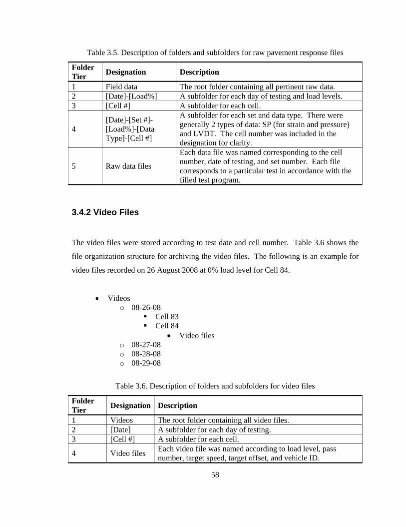
58

Table 3.5. Description of folders and subfolders for raw pavement response files

Folder Tier Designation Description

1 Field data The root folder containing all pertinent raw data. 2 [Date]-[Load%] A subfolder for each day of testing and load levels. 3 [Cell #] A subfolder for each cell.

4 [Date]-[Set #]-[Load%]-[Data Type]-[Cell #]

A subfolder for each set and data type. There were generally 2 types of data: SP (for strain and pressure) and LVDT. The cell number was included in the designation for clarity.

5 Raw data files

Each data file was named corresponding to the cell number, date of testing, and set number. Each file corresponds to a particular test in accordance with the filled test program.

3.4.2 Video Files

The video files were stored according to test date and cell number. Table 3.6 shows the

file organization structure for archiving the video files. The following is an example for

video files recorded on 26 August 2008 at 0% load level for Cell 84.

• Videos o 08-26-08

Cell 83 Cell 84

• Video files o 08-27-08 o 08-28-08 o 08-29-08

Table 3.6. Description of folders and subfolders for video files

Folder Tier Designation Description

1 Videos The root folder containing all video files. 2 [Date] A subfolder for each day of testing. 3 [Cell #] A subfolder for each cell.

4 Video files Each video file was named according to load level, pass number, target speed, target offset, and vehicle ID.

59

3.4.3 Peak-Pick Output

The output files generated from the Peak-Pick analysis was organized in a similar fashion

to the raw data pavement response file structure. In addition to the file structure for raw

data files, two new tiers were added with naming conventions “[Cell #]-[Load Level]-

[Vehicle ID]” and “[Peak-Pick Selection Mode] Results”. The Peak-Pick output result

files should be organized according to the format shown in Table 3.7. An example for

the case of 0% load level, Cell 84, Strain and Stress data, Set 2, Vehicle T6 is shown

subsequently.

• Peak-Pick Results 0% load

• Cell 83 • Cell 84

o 08-24-09_set1_0%_LVDT-C84 o 08-24-09_set1_0%_SP-C84 o 08-24-09_set2_0%_LVDT-C84 o 08-24-09_set2_0%_SP-C84

C84_0%_Mn80 C84_0%_Mn102 C84_0%_R5 C84_0%_T6

• Auto_Results o Peak-Pick auto output files

• Manual_Results o Peak-Pick manual output

files 50% load 100% load 50% load concrete 100% load concrete

60

Table 3.7. Format for folders and subfolders for Peak-Pick output files

Folder Tier Designation Description

1 Peak-Pick Results The root folder containing all pertinent Peak-Pick data.2 [Load%] A subfolder for every load level. 3 [Cell #] A subfolder for each cell.

4 [Date]-[Set #]-[Load%]-[Data Type]-[Cell #]

A subfolder for each set and data type. There are 2 types of data: SP (for strain and pressure) and LVDT. The cell number was included in the designation for clarity.

5 [Cell #]-[Load%]-[Vehicle] A subfolder for each tested vehicle.

6 [P-P Selection Mode]-Results

A subfolder separating auto or manual peak selections in Peak-Pick.

7 P-P output files Generated output files from running Peak-Pick.

61

Chapter 4 Data Analysis

An evaluation of relative pavement damage induced by various types of agricultural

equipments was conducted by comparing measured pavement responses (asphalt strains

and subgrade stresses) generated by these vehicles. This chapter presents the analysis

based on a comparison of the maximum responses obtained from the vehicle passes. As

described in Chapter 3, the Peak-Pick program was used to extract the maximum

responses.

Pavement responses are influenced not only by axle loading, but also other factors

including environmental effects, pavement structure, and vehicle wheel path (traffic

wander). Therefore, these factors should be accounted for in the analysis. The effect of

vehicle traffic wander, seasonal changes, time of testing, pavement structure, vehicle

weight, tire type, and vehicle speed on measured asphalt strains and subgrade stresses are

discussed.

4.1 Effect of Vehicle Traffic Wander

The test program was designed to accommodate the effects of vehicle wheel path. Target

offsets were set at various transverse distances from the fog line that the vehicle operator

was directed to follow. In addition, the actual traffic wander was measured during the

test, as explained in the previous chapters.

The results of the testing confirmed the importance of the traffic wander parameter. It

was observed that traffic wander not only affects the maximum response from the same

vehicle, but also affects which axle would result in the maximum response. Figure 4.1

and Figure 4.2 show an example of maximum asphalt strains and subgrade stresses,

respectively, for five passes generated by vehicle T6 axles at an 80% load level in spring

2009. Note that the horizontal axis in the figures (Rear axle relative offset) denotes the

62

distance from the center of the most rear wheel axle relative to the location of the sensor;

in the case for vehicle T6, the most rear axle is axle 4. It can also be observed that when

the rear axle is centered above a sensor, the front axles pass the sensor with an offset.

Figure 4.1 demonstrates that the maximum asphalt strain generated by T6 was from the

rear axle when the offset was -2 in. For offsets from 11 to 15 in., the maximum asphalt

strains were not only reduced by approximately one-third, but the front axles caused

higher stains that the rear. It can be observed from Figure 4.2 that the maximum

subgrade stress from the T6 vehicle occurred when the offset was 3 in. At this offset and

all others, the last axle caused the maximum stress. However, the magnitude of the

maximum stress dropped sharply when the offset increased to 11 or more inches.

AC Strain (83AE4)

0

50

100

150

200

250

-2 3 11 14 15

Rear axle relative offset [in.]

Stra

in [1

0-6] Axle 1

Axle 2Axle 3Axle 4

Figure 4.1. Asphalt strain axle responses for vehicle T6 at 80% load level

63

Subgrade Stress (83PG4)

0

4

8

12

16

20

-2 3 11 14 15

Rear axle relative offset [in.]

Stre

ss [p

si] Axle 1

Axle 2Axle 3Axle 4

Figure 4.2. Subgrade stress axle responses for vehicle T6 at 80% load level

4.2 Effect of Seasonal Changes

The properties of a pavement structure are dependent on environmental conditions such

as moisture content and temperature. In winter, the saturated base and subgrade layers

would freeze, causing a significant increase in stiffness. As the temperature increases,

the frozen base layer begins to thaw, resulting in an undrained condition as the water

becomes trapped between the impermeable asphalt layer and the frozen subgrade within

the pavement structure. During this period, the cohesionless and saturated base and

subgrade layers will experience a decrease in stiffness and strength as thawing continues.

The overall structural capacity of the pavement will be reduced significantly. This is the

main reason for spring load restrictions in regions experiencing freeze-thaw

environments. Furthermore, the elastic and viscoelastic properties of the asphalt layer are

both susceptible to temperature changes. At low temperatures, asphalt becomes stiff and

behaves as a brittle material. At higher temperatures, the asphalt stiffness is reduced and

the material is more ductile.

64

With these effects in mind, field testing was conducted twice a year in the spring and fall

seasons. Test vehicles were selected based on availability, application frequency, and

recommendations by the industry. Ideally, each vehicle should have been tested at least

once in the spring and once in the fall season. However, due to availability constraints,

this could not be fulfilled. It should be noted that in some instances, a slightly different

type of tractor model was tested in place of the original tractor with the tanker remaining

the same. To maintain consistency, the capacity and axle configuration of these

replacement tractors were aimed to be as similar to the original as possible.

MnROAD standard 80-kip truck Mn80 was used as the control vehicle throughout this

study. Therefore, its pavement responses were used as the reference measurements to

evaluate the effects of seasonal changes on pavement response. It is important to note

that the number of passes made by Mn80 varied for different testing days. Fewer passes

of Mn80 could result in less coverage of different wheel path offsets. This has potential

to ultimately affect the maximum response measurements, since the offset causing the

highest response may not have been covered. The number of passes made by Mn80 on a

particular test day at the flexible pavement section is summarized in Table 4.1. Figure

4.3 through Figure 4.7 show the maximum asphalt strain and subgrade stress values for

each test day from Cells 83 and 84 from Mn80. It can be observed that there are

significant seasonal variations in the measured stresses and strains. In addition, there are

some significant daily fluctuations in the measured responses due to temperature

variation.

65

Table 4.1. Number of passes made by Mn80 at the flexible pavement section

Day Number of PassesS08-day1 2 S08-day2 4 F08-day1 15 F08-day2 20 F08-day3 5 S09-day1 15 S09-day2 13 S09-day3 12 S09-day4 20 F09-day1 29 F09-day2 28 F09-day3 41 F09-day4 44 S10-day1 68 S10-day2 71 S10-day3 72 F10-day1 68 F10-day2 74 TOTAL 601

Mn80 AC Strain (83AE4)

0300600900

120015001800

S08

-day

1

S08

-day

2

F08-

day1

F08-

day2

F08-

day3

S09

-day

1

S09

-day

2

S09

-day

3

S09

-day

4

F09-

day1

F09-

day2

F09-

day3

F09-

day4

S10

-day

1

S10

-day

2

S10

-day

3

F10-

day1

F10-

day2

Test day

Stra

in [1

0-6]

Figure 4.3. Cell 83 angled asphalt strain generated by vehicle Mn80

66

Mn80 AC Strain (84LE4)

0

300

600900

1200

1500

1800

S08

-day

1

S08

-day

2

F08-

day1

F08-

day2

F08-

day3

S09

-day

1

S09

-day

2

S09

-day

3

S09

-day

4

F09-

day1

F09-

day2

F09-

day3

F09-

day4

S10

-day

1

S10

-day

2

S10

-day

3

F10-

day1

F10-

day2

Test day

Str

ain

[10-6

]

Figure 4.4. Cell 84 longitudinal asphalt strain generated by vehicle Mn80

Mn80 AC Strain (84TE4)

0

300

600

900

1200

1500

1800

S08

-day

1

S08

-day

2

F08-

day1

F08-

day2

F08-

day3

S09

-day

1

S09

-day

2

S09

-day

3

S09

-day

4

F09-

day1

F09-

day2

F09-

day3

F09-

day4

S10

-day

1

S10

-day

2

S10

-day

3

F10-

day1

F10-

day2

Test day

Stra

in [1

0-6]

Figure 4.5. Cell 84 transverse asphalt strain generated by vehicle Mn80

67

Mn80 Subgrade Stress (83PG4)

0

5

10

15

20

25

S08

-day

1

S08

-day

2

F08-

day1

F08-

day2

F08-

day3

S09

-day

1

S09

-day

2

S09

-day

3

S09

-day

4

F09-

day1

F09-

day2

F09-

day3

F09-

day4

S10

-day

1

S10

-day

2

S10

-day

3

F10-

day1

F10-

day2

Test day

Stre

ss [p

si]

Figure 4.6. Cell 83 vertical subgrade stress generated by vehicle Mn80

Mn80 Subgrade Stress (84PG4)

0

5

10

15

20

25

S08

-day

1

S08

-day

2

F08-

day1

F08-

day2

F08-

day3

S09

-day

1

S09

-day

2

S09

-day

3

S09

-day

4

F09-

day1

F09-

day2

F09-

day3

F09-

day4

S10

-day

1

S10

-day

2

S10

-day

3

F10-

day1

F10-

day2

Test day

Stre

ss [p

si]

Figure 4.7. Cell 84 vertical subgrade stress generated by vehicle Mn80

Figure 4.3 through Figure 4.5 show that measured asphalt strains were lower in the spring

seasons compared to the fall seasons for both Cells 83 and 84. In the spring, the average

angled strain (strain gage 83AE4) in Cell 83 was only 23% of the average angled strain in

fall. Average longitudinal strain (strain gage 84LE4) in Cell 84 during spring was 34%

of the average longitudinal strain during fall. Average transverse strain (strain gage

68

84TE4) in Cell 84 during spring was 25% of the average transverse strain in fall. This

trend was anticipated, since with warmer pavement temperatures, asphalt stiffness is

reduced, which leads to higher strains. A 2-sample t-test was performed to compare

maximum asphalt strains generated between spring and fall seasons. At a 0.05

significance level, the t-test suggested that the strain responses in the spring were lower

than in the fall. It was also observed that transverse strains were generally larger than

longitudinal strains under vehicle Mn80. The higher strain measurements in fall suggest

that the asphalt layer is more susceptible to fatigue like damage during that season.

The unusually large angled strains in Cell 83 during fall 2009 testing was assumed to be

caused by additional external factors influencing the strain gage. The pavement section

at Cell 83 failed during spring 2009 due to a longitudinal crack, followed by immense

rutting at approximately fifteen feet from the sensor array. The failed section was

repaired in preparation for fall 2009, but once again failed during testing. In this case, the

failure was located approximately four feet from the sensor array. This failure most

likely caused changes within the pavement structure and in turn, affected the material

properties of the structure within close proximity of the strain gage. Conversely, the

pavement section at Cell 84 exhibited no visible damage.

The average maximum subgrade stress in the spring was 90% and 95% of the maximum

stresses in the fall for Cell 83 (earth pressure cell 83PG4) and Cell 84 (earth pressure cell

84PG4), respectively. Although this implies that subgrade stresses were only slightly

higher in fall compared to spring, there were no strong correlations for measured vertical

subgrade stresses with test seasons. Notice that a spike in subgrade stress occurred on

day 1 of spring 2009. A possible explanation for this occurrence is the frequent freeze-

thaw cycle in spring. During spring (or late spring), the frozen base and subgrade layers

should begin to thaw, greatly reducing the stiffness and strength of those layers. The

reason that the spike on day 1 of spring 2009 shows otherwise could be due to the

subgrade layer, which was still frozen. Excluding the spike on day 1 of spring 2009, the

t-test suggested that there was a difference between maximum measured subgrade

69

stresses in the fall and spring seasons at Cell 83, but not at Cell 84. A more thorough

examination should be performed to investigate subgrade stresses as a function of

moisture content within the base and subgrade layers.

The comparisons of the responses from the 80-kip MnROAD truck (Mn80) could not be

reproduced for other agricultural vehicles directly because the vehicle weights were

varied for each day. In order to demonstrate the seasonal effects on pavement responses

for other vehicles, a correction factor was introduced (see section titled “Effect of Vehicle

and Axle Weight”). Apart from the apparent effects of seasonal changes on pavement

responses, the results also suggest that daily fluctuations in asphalt strains and subgrade

stresses exist. The subsequent section examines how temperature changes during the day

affect pavement responses.

4.3 Effect of Time of Testing

The test program was designed to account for changing pavement temperatures as well.

For example, during the time of testing in one day the pavement temperature varied from

80ºF to 87ºF in the fall of 2009 and from 40ºF to 50ºF in the spring of 2009. Since the

asphalt layer properties are highly sensitive to temperature changes, it is crucial to

capture pavement responses generated by these heavy vehicles at various pavement

temperatures. To do so, testing for one day at the same load level was conducted at two

times: in the morning and in the afternoon. By doing so, the larger difference between

pavement temperatures was successfully distinguished, where morning (AM) tests

represented colder temperatures and afternoon (PM) tests represented warmer

temperatures.

For the sake of this comparison, the maximum axle response measurements from each of

the vehicle passes were extracted and plotted against the last axles’ position relative to

the sensor location. Figure 4.8 through Figure 4.11 show the maximum response

distribution across the pavement width relative to the sensor location at Cell 84 for

70

vehicle Mn80 for spring and fall seasons. Figure 4.12 through Figure 4.15 show the

extracted maximum strain and stress responses between morning and afternoon tests for

Cell 84 during spring and fall seasons for tested vehicles.

Mn80 AC Strain (84LE4) S09

0

100

200

300

400

500

600

-25 -15 -5 5 15 25

Rear axle relative offset [in.]

Stra

in [1

0-6]

AMPM

Figure 4.8. Cell 84 longitudinal asphalt strain generated by Mn80 in spring 2009

Mn80 AC Strain (84LE4) F09

0

100

200

300

400

500

600

-25 -15 -5 5 15 25

Rear axle relative offset [in.]

Stra

in [1

0-6]

AMPM

Figure 4.9. Cell 84 longitudinal asphalt strain generated by Mn80 in fall 2009

71

Mn80 Subgrade Stress (84PG4) S09

0

3

6

9

12

15

-25 -15 -5 5 15 25

Rear axle relative offset [in.]

Stre

ss [p

si]

AMPM

Figure 4.10. Cell 84 vertical subgrade stress generated by Mn80 in spring 2009

Mn80 Subgrade Stress (84PG4) F09

0

3

6

9

12

15

-25 -15 -5 5 15 25

Rear axle relative offset [in.]

Stre

ss [p

si]

AMPM

Figure 4.11. Cell 84 vertical subgrade stress generated by Mn80 in fall 2009

72

AC Strain (84LE4) 80% S09

0

50

100

150

200

Mn80 R4 R5 S4 S5 T6 T7 T8

Vehicles

Stra

in [1

0-6]

AMPM

Figure 4.12. Morning and afternoon maximum longitudinal asphalt strains at Cell 84 for

vehicles loaded at 80% load level in spring 2009

AC Strain (84LE4) 100% F09

0

100

200

300

400

500

600

700

Mn102 Mn80 R5 T6 T7 T8

Vehicles

Stra

in [1

0-6]

AMPM

Figure 4.13. Morning and afternoon maximum longitudinal asphalt strains at Cell 84 for

vehicles loaded at 100% load level in fall 2009

73

Subgrade Stress (84PG4) 80% S09

0

5

10

15

20

Mn80 R4 R5 S4 S5 T6 T7 T8

Vehicles

Stre

ss [p

si]

AMPM

Figure 4.14. Morning and afternoon maximum vertical subgrade stresses at Cell 84 for

vehicles loaded at 80% load level in spring 2009

Subgrade Stress (84PG4) 100% F09

0

5

10

15

20

25

Mn102 Mn80 R5 T6 T7 T8

Vehicles

Stre

ss [p

si]

AMPM

Figure 4.15. Morning and afternoon maximum vertical subgrade stresses at Cell 84 for

vehicles loaded at 100% load level in fall 2009

74

Figure 4.8 through Figure 4.11 indicate that Mn80 passes in the afternoon (PM) generate

larger asphalt strains and subgrade stresses compared to tests performed in the morning

(AM). For the same relative offset, longitudinal asphalt strains measured in spring 2009

exhibit a difference of approximately 50% between AM and PM testing. However, the

difference for similar offsets was roughly 30% in fall 2009. On the other hand, recorded

subgrade stresses yielded a 30% difference in spring and 20% difference in fall between

AM and PM testing. It is evident that temperature changes effects both strain and stress

responses. This observation for vehicle Mn80 is a recurring trend for all other tested

vehicles. Figure 4.12 through Figure 4.15 represent the extracted maximum strain and

stress responses generated by the respective vehicles across the pavement width between

morning and afternoon tests. The paired t-test was performed to test the significance

between morning and afternoon responses for agricultural vehicles loaded at 80% and

100 % load levels in spring 2009 and fall 2009 tests, respectively. At a 0.05 significance

level, the t-test suggested that both asphalt strains and subgrade stresses measured in the

spring and fall seasons were indeed larger in the afternoon than in the morning.

Preliminary observations suggest that asphalt strains and subgrade stresses were

significantly lower in the morning than in the afternoon. To be more precise in

evaluating this issue, pavement response measurements should be corrected for asphalt

temperature. Additionally, pavement distress development was not observed during

testing in the morning sessions and significant displacements of the pavement surface

were clearly visible in the afternoon sessions as the loaded agricultural vehicles made

their passes. The pavement cross-section characteristics also influenced pavement

responses as discussed in the next section.

75

4.4 Effect of Pavement Structure

Two flexible pavement sections were constructed specifically for this study at the

MnROAD facility. Table 2.1 describes the structural geometry of the flexible pavement

sections. The objective was to evaluate the effect of asphalt and base layer thicknesses,

as well as shoulder type, on pavement responses. To achieve this objective, the

maximum strain and stress responses across the pavement width were extracted for each

vehicle and compared between Cell 83 (thin section) and Cell 84 (thick section). Due to

failure of longitudinal and transverse strain gages in Cell 83 and angled strain gage in

Cell 84, a comparison between strains with the same orientation was not possible.

Instead, the largest values among the longitudinal and transverse strains from Cell 84

were compared against angled strains from Cell 83. Bar charts in Figure 4.16 through

Figure 4.23 show the measured responses.

AC Strain 80% F08

0

100

200

300

400

500

600

700

Mn80 R4 T6 T7

Vehicles

Stra

in [1

0-6]

Cell 83Cell 84

Figure 4.16. Maximum asphalt strains between Cell 83 and 84 for fall 2008 at 80% load

level

76

Subgrade Stress 80% F08

0

5

10

15

20

25

30

Mn80 R4 T6 T7

Vehicles

Stre

ss [p

si]

Cell 83Cell 84

Figure 4.17. Maximum subgrade stresses between Cell 83 and 84 for fall 2008 at 80%

load level

AC Strain 80% S09

0

50

100

150

200

250

300

Mn80 R4 R5 S4 S5 T6 T7 T8

Vehicles

Stra

in [1

0-6]

Cell 83Cell 84

Figure 4.18. Maximum asphalt strains between Cell 83 and 84 for spring 2009 at 80%

load level

77

Subgrade Stress 80% S09

0

5

10

15

20

25

Mn80 R4 R5 S4 S5 T6 T7 T8

Vehicles

Stre

ss [p

si]

Cell 83Cell 84

Figure 4.19. Maximum subgrade stresses between Cell 83 and 84 for spring 2009 at 80%

load level

AC Strain 100% F09

0

300

600

900

1200

1500

1800

Mn102 Mn80 R5 T6 T7 T8

Vehicles

Stra

in [1

0-6]

Cell 83Cell 84

Figure 4.20. Maximum asphalt strains between Cell 83 and 84 for fall 2009 at 100% load

level

78

Subgrade Stress 100% F09

0

5

10

15

20

25

30

Mn102 Mn80 R5 T6 T7 T8

Vehicles

Stre

ss [p

si]

Cell 83Cell 84

Figure 4.21. Maximum subgrade stresses between Cell 83 and 84 for fall 2009 at 100%

load level

AC Strain 100% S10

0

100

200

300

400

Mn102 Mn80 R6 T6

Vehicles

Str

ain

[10-6

]

Cell 84

Figure 4.22. Maximum asphalt strains of Cell 84 for spring 2010 at 100% load level

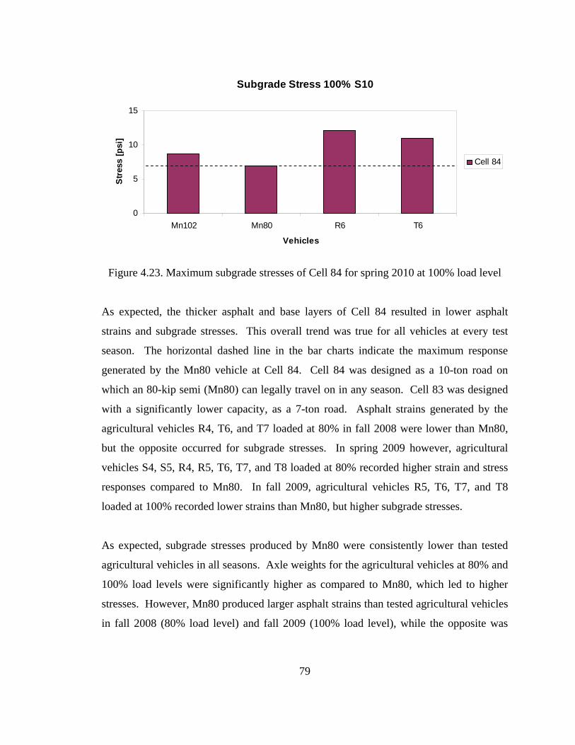
79

Subgrade Stress 100% S10

0

5

10

15

Mn102 Mn80 R6 T6

Vehicles

Str

ess

[psi

]

Cell 84

Figure 4.23. Maximum subgrade stresses of Cell 84 for spring 2010 at 100% load level

As expected, the thicker asphalt and base layers of Cell 84 resulted in lower asphalt

strains and subgrade stresses. This overall trend was true for all vehicles at every test

season. The horizontal dashed line in the bar charts indicate the maximum response

generated by the Mn80 vehicle at Cell 84. Cell 84 was designed as a 10-ton road on

which an 80-kip semi (Mn80) can legally travel on in any season. Cell 83 was designed

with a significantly lower capacity, as a 7-ton road. Asphalt strains generated by the

agricultural vehicles R4, T6, and T7 loaded at 80% in fall 2008 were lower than Mn80,

but the opposite occurred for subgrade stresses. In spring 2009 however, agricultural

vehicles S4, S5, R4, R5, T6, T7, and T8 loaded at 80% recorded higher strain and stress

responses compared to Mn80. In fall 2009, agricultural vehicles R5, T6, T7, and T8

loaded at 100% recorded lower strains than Mn80, but higher subgrade stresses.

As expected, subgrade stresses produced by Mn80 were consistently lower than tested

agricultural vehicles in all seasons. Axle weights for the agricultural vehicles at 80% and

100% load levels were significantly higher as compared to Mn80, which led to higher

stresses. However, Mn80 produced larger asphalt strains than tested agricultural vehicles

in fall 2008 (80% load level) and fall 2009 (100% load level), while the opposite was

80

observed in spring 2009 (80% load level) and spring 2010 (100% load level). An attempt

to explain this phenomenon through the layered elastic theory was unsuccessful.

Plotting the maximum subgrade stress responses from a particular vehicle pass against its

corresponding offset relative to the sensor location reveals an additional effect of the

pavement cross-section. Responses generated by vehicle R5 during spring 2009 at 80%

load level and vehicle T6 during fall 2009 at 100% load level are presented for Cells 83

and 84 in Figure 4.24 through Figure 4.27.

R5 Subgrade Stress (83PG4) 80% S09

0

5

10

15

20

-10 -5 0 5 10 15 20 25

Rear axle relative offset [in.]

Stre

ss [p

si]

AMPM

Figure 4.24. Cell 83 vertical subgrade stress generated by R5 in spring 2009 at 80% load

level

81

R5 Subgrade Stress (84PG4) 80% S09

0

5

10

15

20

-10 -5 0 5 10 15 20 25

Rear axle relative offset [in.]

Stre

ss [p

si]

AMPM

Figure 4.25. Cell 84 vertical subgrade stress generated by R5 in spring 2009 at 80% load

level

T6 Subgrade Stress (83PG4) 100% F09

0

5

10

15

20

25

30

-20 -15 -10 -5 0 5 10 15 20

Rear axle relative offset [in.]

Stre

ss [p

si]

AMPM

Figure 4.26. Cell 83 vertical subgrade stress generated by T6 in fall 2009 at 100% load

level

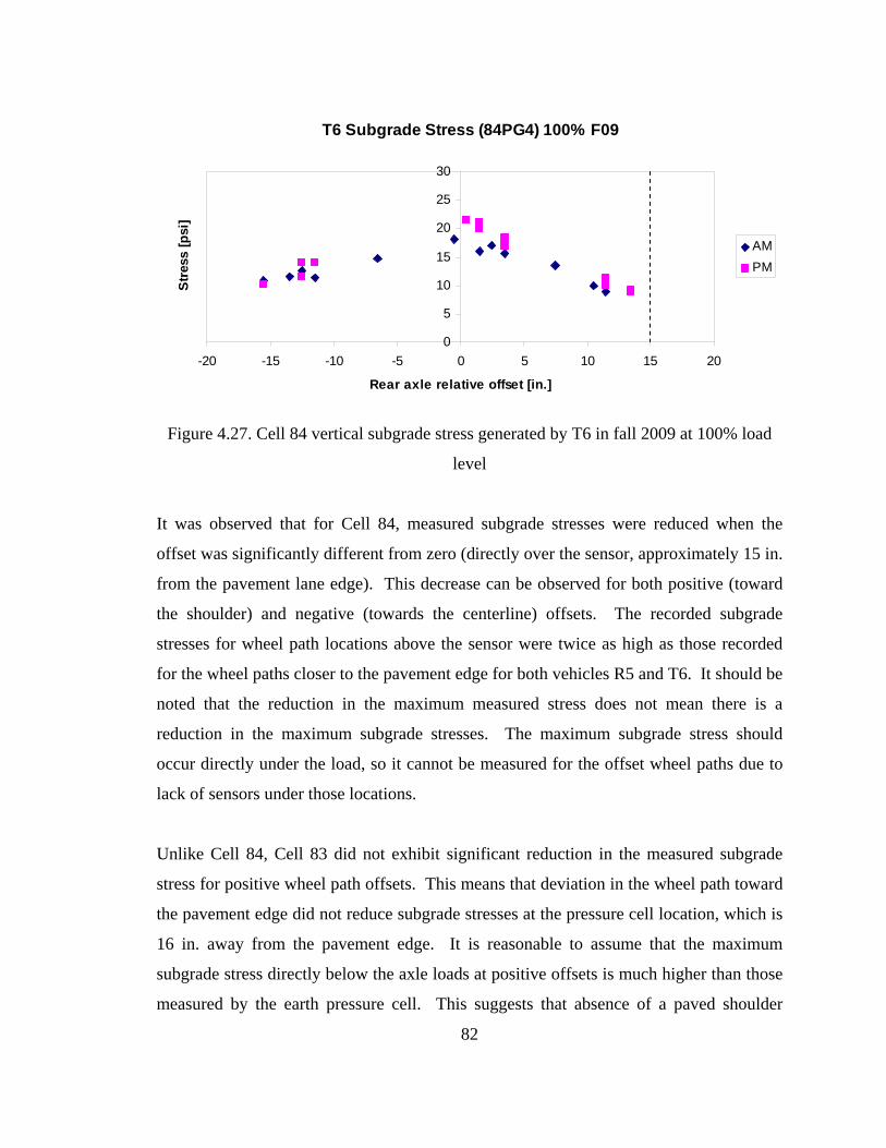
82

T6 Subgrade Stress (84PG4) 100% F09

0

5

10

15

20

25

30

-20 -15 -10 -5 0 5 10 15 20

Rear axle relative offset [in.]

Stre

ss [p

si]

AMPM

Figure 4.27. Cell 84 vertical subgrade stress generated by T6 in fall 2009 at 100% load

level

It was observed that for Cell 84, measured subgrade stresses were reduced when the

offset was significantly different from zero (directly over the sensor, approximately 15 in.

from the pavement lane edge). This decrease can be observed for both positive (toward

the shoulder) and negative (towards the centerline) offsets. The recorded subgrade

stresses for wheel path locations above the sensor were twice as high as those recorded

for the wheel paths closer to the pavement edge for both vehicles R5 and T6. It should be

noted that the reduction in the maximum measured stress does not mean there is a

reduction in the maximum subgrade stresses. The maximum subgrade stress should

occur directly under the load, so it cannot be measured for the offset wheel paths due to

lack of sensors under those locations.

Unlike Cell 84, Cell 83 did not exhibit significant reduction in the measured subgrade

stress for positive wheel path offsets. This means that deviation in the wheel path toward

the pavement edge did not reduce subgrade stresses at the pressure cell location, which is

16 in. away from the pavement edge. It is reasonable to assume that the maximum

subgrade stress directly below the axle loads at positive offsets is much higher than those

measured by the earth pressure cell. This suggests that absence of a paved shoulder

83

significantly increases the maximum subgrade stresses when the wheel path is near the

pavement edge, as illustrated in Figure 4.28.

Figure 4.28. Cross-section view of pave and unpaved sections

A similar effect was observed for asphalt strains. Figure 4.29 through Figure 4.34 show

that when the wheel path was translated toward the shoulder and away from the sensor,

the measured asphalt strains in Cell 84 were significantly reduced. However, measured

strains for Cell 83 were not reduced for similar loading conditions. For vehicle R5, strain

responses were decreased by approximately 7% as the wheel path approached the

pavement edge for Cell 83. For Cell 84 longitudinal strain, the decrease was roughly

50% and 70% for transverse strain. For vehicle T6, the decrease in angle strain for Cell

83 was only 2% and the decrease for Cell 84 longitudinal strain was approximately 25%.

For the transverse strain in Cell 84, there was an increase of 4% as the vehicle’s wheel

path approached the pavement edge. The difference in responses of Cells 83 and 84 for

different wheel path locations are due to the effect of different pavement shoulders. Cell

83 has an aggregate shoulder and Cell 84 has an asphalt shoulder. Cell 83, which has an

aggregate shoulder, experienced higher coverage of the critical responses at the sensor

location than Cell 84. This clearly demonstrates the importance of the structural benefits

of the asphalt shoulder.

P1a P2a P1b P2b

Sensor 84PG4Sensor 83PG4

Paved Shoulder (Cell 84) Aggregate Shoulder (Cell 83)

AC layer AC layer

P1a = P2a P1b = P2b

84

R5 AC Strain (83AE4) 80% S09

0

50

100

150

200

-10 -5 0 5 10 15 20 25

Rear axle relative offset [in.]

Str

ain

[10-6

]

AMPM

Figure 4.29. Cell 83 angled asphalt strain generated by R5 in spring 2009 at 80% load

level

R5 AC Strain (84LE4) 80% S09

0

50

100

150

200

-10 -5 0 5 10 15 20 25

Rear axle relative offset [in.]

Stra

in [1

0-6]

AMPM

Figure 4.30. Cell 84 longitudinal asphalt strain generated by R5 in spring 2009 at 80%

load level

85

R5 AC Strain (84TE4) 80% S09

0

50

100

150

200

-10 -5 0 5 10 15 20 25

Rear axle relative offset [in.]

Str

ain

[10-6

]

AMPM

Figure 4.31. Cell 84 transverse asphalt strain generated by R5 in spring 2009 at 80% load

level

T6 AC Strain (83AE4) 100% F09

0

500

1000

1500

-20 -15 -10 -5 0 5 10 15 20

Rear axle relative offset [in.]

Stra

in [1

0-6]

AMPM

Figure 4.32. Cell 83 angled asphalt strain generated by T6 in fall 2009 at 100% load level

86

T6 AC Strain (84LE4) 100% F09

0

500

1000

1500

-20 -15 -10 -5 0 5 10 15 20

Rear axle relative offset [in.]

Stra

in [1

0-6]

AMPM

Figure 4.33. Cell 84 longitudinal asphalt strain generated by T6 in fall 2009 at 100% load

level

T6 AC Strain (84TE4) 100% F09

0

500

1000

1500

-20 -15 -10 -5 0 5 10 15 20

Rear axle relative offset [in.]

Str

ain

[10-6

]

AMPM

Figure 4.34. Cell 84 transverse asphalt strain generated by T6 in fall 2009 at 100% load

level

87

4.5 Effect of Vehicle and Axle Weight

4.5.1 Effect of Vehicle Weight

The pavement responses in Cell 84 from vehicles S5 for spring 2009 and T6 for fall 2009

are presented in Figure 4.35 through Figure 4.40. The maximum strain and stress

responses from a particular vehicle pass were plotted against its corresponding offset

relative to the sensor location. Figure 4.35 through Figure 4.37 show the response

measurements for vehicle S5, and Figure 4.38 through Figure 4.40 for vehicle T6. Gross

vehicle weights are shown in the legends.

S5 AC Strain (84LE4) S09

0

50

100

150

200

-10 -5 0 5 10 15 20 25 30

Rear axle relative offset [in.]

Stra

in [1

0-6] 25 kip

34 kip43 kip55 kip

Figure 4.35. Cell 84 longitudinal asphalt strain generated by S5 in spring 2009 at various

gross weights

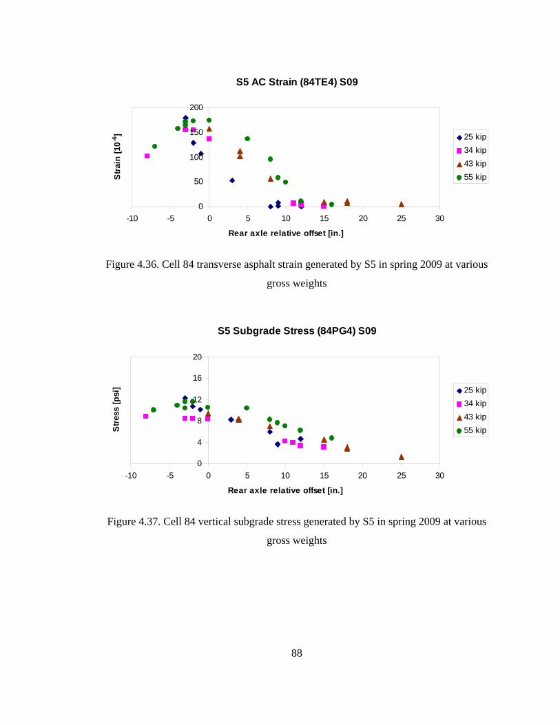
88

S5 AC Strain (84TE4) S09

0

50

100

150

200

-10 -5 0 5 10 15 20 25 30

Rear axle relative offset [in.]

Stra

in [1

0-6] 25 kip

34 kip43 kip55 kip

Figure 4.36. Cell 84 transverse asphalt strain generated by S5 in spring 2009 at various

gross weights

S5 Subgrade Stress (84PG4) S09

0

4

8

12

16

20

-10 -5 0 5 10 15 20 25 30

Rear axle relative offset [in.]

Stre

ss [p

si] 25 kip

34 kip43 kip55 kip

Figure 4.37. Cell 84 vertical subgrade stress generated by S5 in spring 2009 at various

gross weights

89

T6 AC Strain (84LE4) F09

0

200

400

600

800

-20 -15 -10 -5 0 5 10 15 20 25

Rear axle relative offset [in.]

Stra

in [1

0-6]

40 kip64 kip90 kip

Figure 4.38. Cell 84 longitudinal asphalt strain generated by T6 in fall 2009 at various

gross weights

T6 AC Strain (84TE4) F09

0

200

400

600

800

-20 -15 -10 -5 0 5 10 15 20 25

Rear axle relative offset [in.]

Stra

in [1

0-6]

40 kip64 kip90 kip

Figure 4.39. Cell 84 transverse asphalt strain generated by T6 in fall 2009 at various

gross weights

90

T6 Subgrade Stress (84PG4) F09

0

5

10

15

20

25

-20 -15 -10 -5 0 5 10 15 20 25

Rear axle relative offset [in.]

Stre

ss [p

si]

40 kip64 kip90 kip

Figure 4.40. Cell 84 vertical subgrade stress generated by T6 in fall 2009 at various gross

weights

It can be observed that longitudinal and transverse strain responses generated by vehicle

S5 (Figure 4.35 and Figure 4.36) steadily increase as vehicle weight increases. However,

subgrade stresses for vehicle S5 for a gross weight of 25,000 lb (25 kip) were larger than

at 55,000 lb (55 kip). This can be explained by referring to Figure 4.7 from the “Effect of

Seasonal Changes” section, which clearly shows a spike on the first day of spring 2009

testing for the Mn80 truck. This test day corresponds to the same day in which vehicle

S5 was tested at 25 kip. Measurements collected on that day also resulted in the same

trend for the other vehicles. An increase in longitudinal strains and subgrade stresses as

vehicle weight increased was also observed for vehicle T6 in fall 2009, as shown in

Figure 4.38 and Figure 4.40, respectively. Responses for transverse strains however were

not as clear and no strong correlation was observed between transverse strains with gross

vehicle weight for T6. Overall, there was an increase in stresses and strains as vehicle

weight increased. However, it should be noted that tests for different vehicle weights

(load levels) were conducted on different days, hence daily fluctuations and seasonal

effects should be considered. Strain responses in spring were typically much “cleaner”

compared to fall, and this may be due to several factors, including change in

characteristics of the asphalt layer, frequency of vehicle passes, and time interval between

91

vehicle passes. It should be noted that the figures represent the maximum responses from

the vehicles, and not from individual axles. An increase in gross vehicle weight did not

lead to a proportional increase in axle weight, as will be discussed in subsequent sections.

4.5.2 Effect of Vehicle Type

Testing was conducted with the agricultural vehicles loaded at different load levels: 0%,

25%, 50%, 80%, and 100% of full tank capacity, while control vehicles Mn80 and

Mn102 remained at the same weight. Weights of all vehicles were measured for every

load level and this information is summarized in Appendix B. Table 4.2 and Table 4.3

summarize the gross weight of the vehicles for spring 2009 and fall 2009, respectively.

This section focuses on changes in pavement responses as vehicle weight changes. An

increase in vehicle weight should be reflected by an increase in pavement responses. As

stated previously, pavement responses for vehicle Mn80 at Cell 84 were used as a

benchmark to compare responses for other vehicles. Figure 4.41 through Figure 4.46

show the maximum strain and stress responses for agricultural vehicles for spring 2009

and fall 2009 at Cell 84.

Table 4.2. Gross weight for vehicles tested during spring 2009

Gross Vehicle Weight [lb] Vehicle 0% 25% 50% 80%

S4 27,860 36,260 46,980 57,580 S5 25,180 34,040 42,940 54,840 R4 36,520 41,180 48,060 53,240 R5 31,480 35,520 39,600 43,740 T6 38,780 50,620 63,240 70,220 T7 58,540 72,840 88,050 103,600 T8 58,900 80,340 102,080 123,840

Mn80 79,560

92

Table 4.3. Gross weight for vehicles tested during fall 2009

Gross Vehicle Weight [lb] Vehicle 0% 50% 80%

R5 31,730 39,950 47,100 T6 39,710 64,400 89,500 T7 45,100 75,600 105,200 T8 58,200 97,600 134,200

Mn80 81,090

Analysis of Figure 4.41 through Figure 4.46 shows that, as a general trend, an increase in

vehicle weight leads to an increase in pavement responses. However, this increase is not

proportional to the increase in vehicle weight, and for some vehicles, the responses

decreased when the vehicle weight increased. Several factors may have contributed to

this trend:

• Since different vehicle weights were conducted on different days, the climatic

factors such as temperature could have affected the results. Vehicle Mn80 will be

used later to adjust the results for this effect.

• The increase in gross vehicle weight does not lead to a proportional increase in

vehicle axle weights. As can be observed from Table 4.4, an increase in gross

weight for vehicle T6 significantly affects axle weights for the 3rd and 4th axles,

while the 1st and 2nd axles are mostly unaffected. Moreover, the second axle has

the highest axle weight for 0%, 25%, and 50%, while the 4th axle has the highest

weight for 80% load level. The maximum responses shown in Figure 4.41

through Figure 4.46 can be produced by various axles for different load levels.

Table 4.4. Vehicle T6 axle weights at various load levels

0% 25% 50% 80% Axle [lb] [lb] [lb] [lb]

Axle 1 13,220 12,660 11,940 11,600 Axle 2 17,600 17,700 20,860 22,420 Axle 3 7,140 12,420 16,620 22,440 Axle 4 7,900 13,760 19,760 26,640 Total 45,860 56,540 69,180 83,100

93

AC Strain (84LE4) S09

0

50

100

150

200

250

300

0% 25% 50% 80%

Load Level [%]

Stra

in [1

0-6]

Mn80R4R5S4S5T6T7T8

Figure 4.41. Longitudinal asphalt strain at Cell 84 generated by vehicles tested at 0%,

25%, 50%, and 80% in spring 2009

AC Strain (84TE4) S09

0

50

100

150

200

250

300

0% 25% 50% 80%

Load Level [%]

Str

ain

[10-6

]

Mn80R4R5S4S5T6T7T8

Figure 4.42. Transverse asphalt strain at Cell 84 generated by vehicles tested at 0%, 25%,

50%, and 80% in spring 2009

94

Subgrade Stress (84PG4) S09

0

5

10

15

20

25

30

35

0% 25% 50% 80%

Load Level [%]

Str

ess

[psi

]Mn80R4R5S4S5T6T7T8

Figure 4.43. Vertical subgrade stress at Cell 84 generated by vehicles tested at 0%, 25%,

50%, and 80% in spring 2009

AC Strain (84LE4) F09

0

200

400

600

800

1000

1200

0% 50% 100%

Load Level [%]

Stra

in [1

0-6] Mn80

R5T6T7T8

Figure 4.44. Longitudinal asphalt strain at Cell 84 generated by vehicles tested at 0%,

50%, and 100% in fall 2009

95

AC Strain (84TE4) F09

0

200

400

600

800

1000

1200

0% 50% 100%

Load Level [%]

Stra

in [1

0-6] Mn80

R5T6T7T8

Figure 4.45. Transverse asphalt strain at Cell 84 generated by vehicles tested at 0%, 50%,

and 100% in fall 2009

Subgrade Stress (84PG4) F09

0

5

10

15

20

25

0% 50% 100%

Load Level [%]

Stre

ss [p

si] Mn80

R5T6T7T8

Figure 4.46. Vertical subgrade stress at Cell 84 generated by vehicles tested at 0%, 50%,

and 100% in fall 2009

One of the objectives of this study was to compare pavement responses from various

agricultural vehicles to a standard 5-axle 80-kip semi truck, which was represented by the

Mn80 vehicle. Figure 4.41 through Figure 4.46 show that agricultural vehicles tested in

96

this study at 80% and 100% of full capacity produce higher subgrade stresses (84PG4)

compared to the standard 5-axle 80-kip semi truck (Mn80) in both spring and fall

seasons. An increase in subgrade stresses compared to Mn80 ranged from 4% to 80% in

spring 2009 and 35% to 80% in fall 2009 for agricultural vehicles loaded over 80% load

level. On the other hand, asphalt strain levels generated by the agricultural vehicles were

dependent on test season. In spring, both longitudinal (84LE4) and transverse (84TE4)

strains generated by Mn80 were typically smaller than the agricultural vehicles except for

vehicle T6 for 84LE4 and vehicles R4 and R5 for 84TE4, even at 100% load capacity. In

the fall, this trend was reversed with Mn80 producing larger strains than the other

agricultural vehicles. In the spring of 2009, the S4 and T7 vehicles resulted in asphalt

strains 20% and 48% higher than the Mn80 truck strains, respectively. In fall 2009, the

difference in asphalt strain between vehicle T7 and Mn80 truck was -20%. An attempt to

explain this trend using layered elastic analysis was not successful. Comparisons

between the pavement responses across the pavement width generated by the agricultural

vehicles and Mn80 are presented in Appendix D.

4.5.3 Effect of the Number of Axles

In the past decade, vehicle manufacturers of the agricultural industry began to design and

produce larger equipment with larger capacities. However, in order to be operating

legally on public roads, weight restrictions must be met. To achieve this goal, vehicles

are equipped with additional axles. In this study, the responses from vehicles T6, T7, and

T8 shown in Figure 4.47, were compared. These vehicles are equipped with four, five,

and six total axles, respectively, and have tank capacities of 6,000 gallons, 7,300 gallons,

and 9,500 gallons, respectively. Table 4.5 shows the axle weights of these vehicles

loaded up to 100% when tested in fall 2009. Figure 4.48 shows the vertical subgrade

stress responses at Cell 84 generated by those three vehicles.

97

T6 – 4 axles (John Deere 8230, 6,000 gal) T7 - 5 axles (Case IH 335, 7,300 gal)

T8 – 6 axles (Case IH 335, 9,500 gal)

Figure 4.47. Vehicles with increasing tank capacity and axle number

Table 4.5. Axle weights of vehicles T6, T7, and T8 at 100% in fall 2009

T6 (6,000 gal) T7 (7,300 gal) T8 (9,500 gal)Equipment Axle [lb] [lb] [lb]

Axle 1 8,100 6,900 14,800 Tractor Axle 2 21,400 19,800 25,200 Axle 3 26,500 26,300 23,300 Axle 4 33,500 26,200 23,700 Axle 5 26,000 23,500 Tanker

Axle 6 23,700 Gross vehicle weight 89,500 105,200 134,200

98

Tankers Subgrade Stress (84PG4) F09 100%

0

5

10

15

20

25

-25 -20 -15 -10 -5 0 5 10 15 20

Rear axle relative offset [in.]

Stre

ss [p

si]

T6T7T8

Figure 4.48. Cell 84 vertical subgrade stress generated by vehicles T6, T7, and T8 at

100% load level in fall 2009

Analysis of Table 4.5 shows that although the gross weight of T6 is the lowest amongst

these vehicles, its last axles exhibited the highest load (33,500 lb). Vehicle T8 had the

highest gross weight. However, since the tanker had four axles, each of them resulted in

a relatively low axle weight of 23,700 lb. It is interesting to note that the most loaded

axle was not an axle on the tanker, but rather a rear tractor axle (axle two), which had a

weight of 25,200 lb. As should be expected, vehicle T6 resulted in the highest subgrade

stress while vehicle T8 resulted in the lowest subgrade stress.

Referring to Table 4.5, note that the first two axles for all three vehicles belong to the

tractor. The axle weights of interest here are those belonging to the tankers, which are

axles three to six. Increasing the tank capacity evidently increases the overall vehicle

weight. By adding axles to the tankers, the weight per axle was successfully decreased

with vehicle T6 having the heaviest tanker axle at 33,500 lb, T7 at 26,300 lb, and T8 at

23,700 lb. Figure 4.43 and Figure 4.46 show that vertical subgrade stresses for T6 was

largest, followed by T7 and finally T8 for both spring 2009 and fall 2009 test. Figure

4.48 clearly shows that vehicle T6 generates larger subgrade stresses than the other two

vehicles. Hence, for a larger tank capacity, equipping the tanker with additional axles

99

can potentially reduce the subgrade stresses. Unfortunately, a similar trend was not

observed for asphalt strains. It is worth mentioning that this comparison may not

accurately describe the benefits of having additional axles, since the tankers of vehicles

T6, T7, and T8 were of non-similar sizes.

4.5.4 Effect of Axle Weight

As was discussed, the effect of gross vehicle weight on pavement responses did not show

consistent results. This was attributed to several factors: 1) an increase in gross vehicle

weight is not proportionally distributed to the axle weights; 2) the maximum response

may be generated by different axles; and 3) different vehicle weights were tested on

different days under different temperature conditions. To account for the effect of axle

weight, the response from the rear axle of vehicle T6 was analyzed. A simple correction

factor, di, was introduced to account for climatic effects. This correction factor is based

on responses obtained from the control vehicle Mn80.

i

iT

iMn

oMniTiT d

6

80

8066

σσσ

σσ =⎟⎟⎠

⎞⎜⎜⎝

⎛=) Eqn 4.1

where iT 6σ) is the adjusted subgrade stress from the rear axle of vehicle T6 for ith day

iT 6σ is the measured subgrade stress from the rear axle of vehicle T6 on ith day

oMn80σ is the reference subgrade stress for vehicle Mn80

iMn80σ is the measured subgrade stress for vehicle Mn80 on ith day

id is the ratio between measured subgrade stress on ith day and reference stress

for vehicle Mn80

A similar equation was used to determine adjusted strain values by substituting strain

measurements for stress measurements in Eqn 4.1. To maintain consistency, the

correction factor is always based on the responses generated by the heaviest axle of

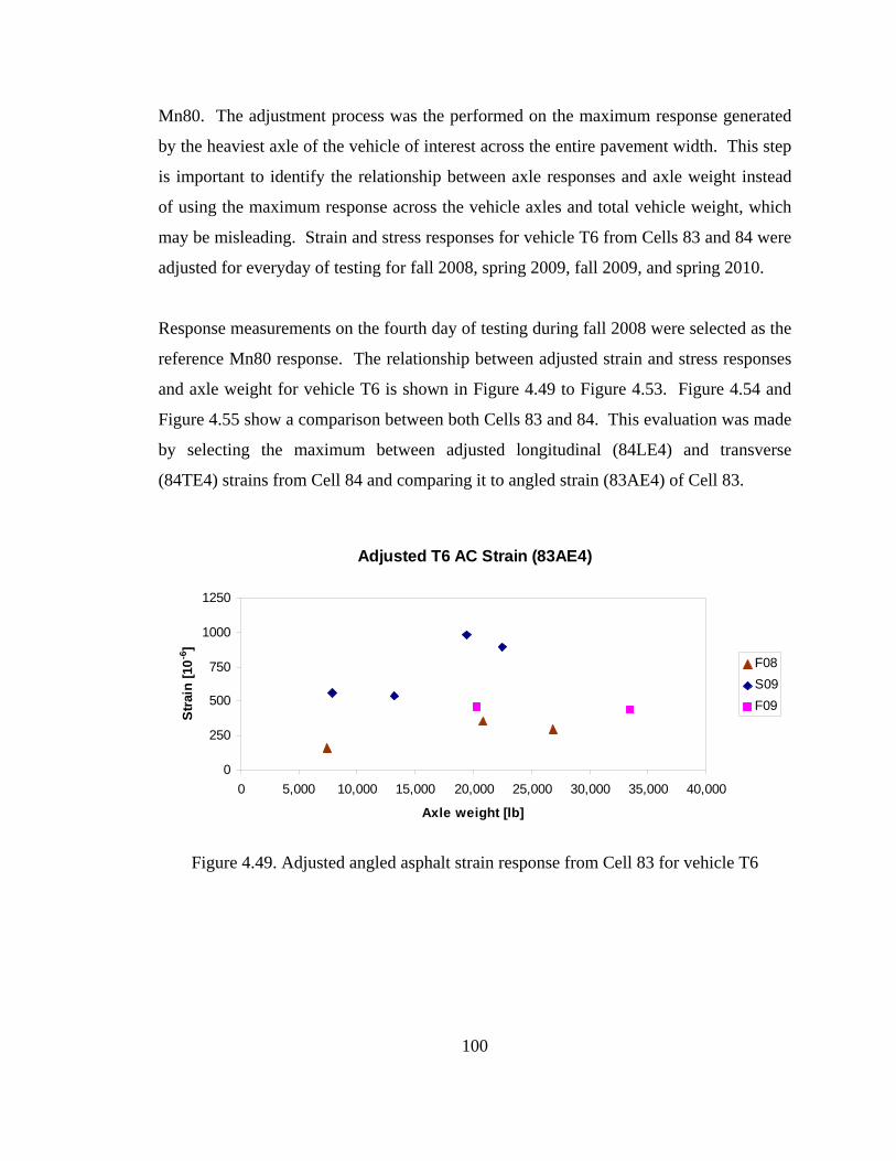
100

Mn80. The adjustment process was the performed on the maximum response generated

by the heaviest axle of the vehicle of interest across the entire pavement width. This step

is important to identify the relationship between axle responses and axle weight instead

of using the maximum response across the vehicle axles and total vehicle weight, which

may be misleading. Strain and stress responses for vehicle T6 from Cells 83 and 84 were

adjusted for everyday of testing for fall 2008, spring 2009, fall 2009, and spring 2010.

Response measurements on the fourth day of testing during fall 2008 were selected as the

reference Mn80 response. The relationship between adjusted strain and stress responses

and axle weight for vehicle T6 is shown in Figure 4.49 to Figure 4.53. Figure 4.54 and

Figure 4.55 show a comparison between both Cells 83 and 84. This evaluation was made

by selecting the maximum between adjusted longitudinal (84LE4) and transverse

(84TE4) strains from Cell 84 and comparing it to angled strain (83AE4) of Cell 83.

Adjusted T6 AC Strain (83AE4)

0

250

500

750

1000

1250

0 5,000 10,000 15,000 20,000 25,000 30,000 35,000 40,000

Axle weight [lb]

Stra

in [1

0-6]

F08S09F09

Figure 4.49. Adjusted angled asphalt strain response from Cell 83 for vehicle T6

101

Adjusted T6 Subgrade Stress (83PG4)

0

10

20

30

40

0 5,000 10,000 15,000 20,000 25,000 30,000 35,000 40,000

Axle weight [lb]

Stre

ss [p

si]

F08S09F09

Figure 4.50. Adjusted vertical subgrade stress response from Cell 83 for vehicle T6

Adjusted T6 AC Strain (84LE4)

0

200

400

600

800

0 5,000 10,000 15,000 20,000 25,000 30,000 35,000 40,000

Axle weight [lb]

Stra

in [1

0-6] F08

S09F09S10

Figure 4.51. Adjusted longitudinal asphalt strain response from Cell 84 for vehicle T6

102

Adjusted T6 AC Strain (84TE4)

0

200

400

600

800

0 5,000 10,000 15,000 20,000 25,000 30,000 35,000 40,000

Axle weight [lb]

Stra

in [1

0-6] S09

F09F08S10

Figure 4.52. Adjusted transverse asphalt strain response from Cell 84 for vehicle T6

Adjusted T6 Subgrade Stress (84PG4)

0

5

10

15

20

25

0 5,000 10,000 15,000 20,000 25,000 30,000 35,000 40,000

Axle weight [lb]

Stre

ss [p

si] S09

F09F08S10

Figure 4.53. Adjusted vertical subgrade stress response from Cell 84 for vehicle T6

103

Adjusted T6 AC Strain

0

250

500

750

1000

1250

0 5,000 10,000 15,000 20,000 25,000 30,000 35,000 40,000

Axle weight [lb]

Stra

in [1

0-6]

Cell 83Cell 84

Figure 4.54. Adjusted asphalt strain responses for vehicle T6 between Cells 83 and 84

Adjusted T6 Subgrade Stress

0

10

20

30

40

0 5,000 10,000 15,000 20,000 25,000 30,000 35,000 40,000

Axle weight [lb]

Stre

ss [p

si]

Cell 83Cell 84

Figure 4.55. Adjusted subgrade stress responses for vehicle T6 between Cells 83 and 84

The purpose of this exercise was to negate daily fluctuations in measured responses. It

was observed that adjusted subgrade stress responses for vehicle T6 from both Cells 83

and 84 have a linear relationship with axle weight, where a stronger linear correlation

exists for Cell 84. Adjusted asphalt strains from Cells 83 and 84 increase with increasing

axle weight. However, there is a significant scatter and the relationship is nonlinear. A

104

possible explanation is the effect of traffic wander and higher sensitivity to temperature

effect that cannot be accounted for with a simple adjustment such as the one described

above. This effect requires further investigation.

4.6 Effect of Tire Type

In the agricultural industry, flotation tires are becoming increasingly popular due to their

wider footprint and lower inflation pressure, which allows the vehicle to travel over soil

and unbound aggregate material with minimal compaction and rutting. With a wider

footprint coupled with low inflation pressure, the wheel load is distributed over a larger

area, thus reducing the stress applied to the soil. This has proved to be beneficial in the

industry where less soil compaction and rutting decreases soil damage. An issue arises as

to whether this characteristic can be translated directly to pavement performance.

In this section, two similar straight trucks with the same tank capacity of 4,400 gallons

were fitted with two different tire types on the tanks, one with regular radial ply dual tire

configuration (Vehicle S4), and the other with a flotation single tire configuration

(Vehicle S5) as shown in Figure 4.56. Comparisons were made using contact area and

contact stress measurements from Tekscan. Additionally, asphalt strains and subgrade

stresses produced by these two vehicles were evaluated.

(a) (b)

Figure 4.56. Straight trucks denoted as (a) vehicle S4 fitted with radial tires (b) vehicle

S5 fitted with flotation tires

105

Tekscan measurements for both vehicles S4 and S5 were taken at load levels of 0%, 50%,

and 80%. Because of the size constraint of the Tekscan equipment, only one side of each

vehicle axle was recorded. The measurements were then calibrated with the actual wheel

load corresponding to the load level. Table 4.6 summarizes the Tekscan results for both

S4 and S5. In order to visualize the growth in contact area and change in contact stress as

wheel load increases, plots were prepared as shown in Figure 4.57 and Figure 4.58.

Additionally, an illustration of how the contact areas of the third axle for both vehicles

change with increasing axle weight is shown in Figure 4.59.

Table 4.6. Tekscan summary for vehicle S4 and S5

Load Level

Wheel Load

Contact Area

Average Stress Vehicle

[%] Axle Filename

[lb] Frame

[in.2] [psi] 0 1 S2_A1LA 5,580 7 56.89 98.1 0 2 S2_A2-3LB 3,680 26 52.41 70.2 0 3 S2_A2-3LB 3,400 45 44.35 76.7 50 1 S2_A1RC50 6,040 211 68.54 88.1 50 2 S2_A2-3RD50 7,800 18 96.31 81 50 3 S2_A2-3RC50 8,040 30 104.38 77 80 1 S2_A1RB80 6,460 30 79.74 81 80 2 S2_A2-3RA80 9,680 85 103.03 94

S4

80 3 S2_A2-3RB80 10,300 98 126.77 81.2 0 1 S1_A1LA 6,400 16 72.57 88.2 0 2 S1_A2-3LA 4,300 10 51.52 83.5 0 3 S1_A2-3LA 3,460 21 50.62 68.4 50 1 S1_A1RA50 7,900 51 81.53 96.9 50 2 S1_A2-3RA50 7,500 50 83.77 89.5 50 3 S1_A2-3RB50 8,390 76 103.48 81.1 80 1 S1_A1RA80 8,780 54 89.14 98.5 80 2 S1_A2-3RA80 9,980 22 105.72 94.4

S5

80 3 S1_A2-3RA80 10,000 33 136.63 73.2

106

Contact Area

0

40

80

120

160

0 2,000 4,000 6,000 8,000 10,000 12,000

Wheel load [lb]

Area

[in.

2 ] S4, radialsS5, flotationsLinear (S4, radials)Linear (S5, flotations)

Figure 4.57. Contact area measurements for vehicles S4 and S5

Average Contact Stress

0

40

80

120

0 2,000 4,000 6,000 8,000 10,000 12,000

Wheel load [lb]

Stre

ss [p

si] S4, radials

S5, flotationsLinear (S4, radials)Linear (S5, flotations)

Figure 4.58. Average contact stress measurements for vehicles S4 and S5

107

S4 – Axle 3 – 8,700 lb S4 – Axle 3 – 16,280 lb S4 – Axle 3 – 21,460 lb

S5 – Axle 3 – 7,100 lb S5 – Axle 3 – 15,340 lb S5 – Axle 3 – 20,040 lb

Figure 4.59. Measured footprints for the third axle of vehicle S4 and S5 with corresponding axle weight

108

Vehicles S4 and S5 are equipped with tires that can deform under load and still maintain

their structural capacity. Regular radial ply dual tires fitted onto vehicle S4 and flotation

tires fitted onto vehicle S5 demonstrate an increase in contact area as the wheel load

increases. A trendline fitted across the data points in Figure 4.57 shows that both tire

types were similar in terms of contact area growth. The average contact stress for both

vehicles also increased with wheel load levels, but the increase was not as significant

because of the larger contact area. There was no significant difference between the two

tire types, as shown in Figure 4.58.

Recognizing that the contact area and average contact stress for both vehicles were very

similar, the pavement response measurements were also evaluated to distinguish any

benefits of flotation tires on pavement performance. To accomplish this comparison, the

analysis was performed by excluding responses generated by the steering axles of both

these vehicles. This ensures that the comparison was made exclusively between radial

and flotation tires on the vehicles’ tanks. Table 4.7 shows the total tank weights for both

vehicles S4 and S5. Figure 4.60 through Figure 4.67 show Cells 83 and 84 pavement

responses generated at load levels of 0% and 80% during spring 2009.

Table 4.7. Tank weights for vehicles S4 and S5

Load Level S4’s Tank S5’s Tank0% 15,180 lb 14,040 lb 80% 40,980 lb 39,440 lb

109

Subgrade Stress (83AE4) 0% S09

0

50

100

150

200

-15 -10 -5 0 5 10 15 20

Rear axle relative offset [in.]

Str

ain

[10-6

]

S4S5

Figure 4.60. Cell 83 angled asphalt strain generated at 0% load level for vehicles S4 and

S5

Subgrade Stress (83PG4) 0% S09

0

2

4

6

8

10

-15 -10 -5 0 5 10 15 20

Rear axle relative offset [in.]

Stre

ss [p

si]

S4S5

Figure 4.61. Cell 83 vertical subgrade stress generated at 0% load level for vehicles S4

and S5

110

Subgrade Stress (84LE4) 0% S09

0

50

100

150

200

-15 -10 -5 0 5 10 15 20

Rear axle relative offset [in.]

Stra

in [1

0-6]

S4S5

Figure 4.62. Cell 84 longitudinal asphalt strain generated at 0% load level for vehicles S4

and S5

Subgrade Stress (84PG4) 0% S09

0

2

4

6

8

10

-15 -10 -5 0 5 10 15 20

Rear axle relative offset [in.]

Stre

ss [p

si]

S4S5

Figure 4.63. Cell 84 vertical subgrade stress generated at 0% load level for vehicles S4

and S5

111

AC Strain (83AE4) 80% S09

0

50

100

150

200

250

-10 -5 0 5 10 15 20

Rear axle relative offset [in.]

Stra

in [1

0-6]

S4S5

Figure 4.64. Cell 83 angled asphalt strain generated at 80% load level for vehicles S4 and

S5

Subgrade Stress (83PG4) 80% S09

0

3

6

9

12

15

-10 -5 0 5 10 15 20

Rear axle relative offset [in.]

Stre

ss [p

si]

S4S5

Figure 4.65. Cell 83 vertical subgrade stress generated at 80% load level for vehicles S4

and S5

112

AC Strain (84LE4) 80% S09

0

50

100

150

200

250

-10 -5 0 5 10 15 20

Rear axle relative offset [in.]

Stra

in [1

0-6]

S4S5

Figure 4.66. Cell 84 longitudinal asphalt strain generated at 80% load level for vehicles

S4 and S5

Subgrade Stress (84PG4) 80% S09

0

3

6

9

12

15

-10 -5 0 5 10 15 20

Rear axle relative offset [in.]

Stre

ss [p

si]

S4S5

Figure 4.67. Cell 84 vertical subgrade stress generated at 80% load level for vehicles S4

and S5

Results show that vehicle S4 produces larger asphalt strains and subgrade stresses at 0%

load levels on both Cells 83 and 84. When loaded to 80%, maximum asphalt strains of

both vehicles at Cell 83 remain similar, but the distribution across the pavement width

was not. Maximum responses for vehicle S5 were recorded when the vehicles’ wheel

113

path was close to the sensor. For vehicle S4, the maximum occurs when the wheel path

was toward the pavement shoulder (positive direction). At Cell 84, the response

distributions across the pavement width show a decreasing trend, as both vehicles travel

away from the sensor toward the shoulder. This not only shows the benefits of a paved

shoulder, but also allows for a more objective representation between responses of both

vehicles S4 and S5. Although maximum values were approximately similar, vehicle S4

was observed to consistently produce slightly larger strains and stresses across the

pavement width.

The observed pavement response distributions in Cell 83 can be attributed to the

difference in axle configuration between the two vehicles. Vehicle S4 was equipped with

dual radial tires whereas S5 was equipped with a single flotation tire on one side of an

axle. Because of the dual tire configuration (the half axle load is applied onto two

separate wheels) the observed response distribution for vehicle S4 occurred when one

side of the dual tires is completely on the aggregate shoulder and the other on the asphalt

pavement. On the other hand, the center of the applied load of vehicle S5 was confined

within the footprint of a single flotation tire, which allows for a more uniform distribution

of the vehicle weight.

114

4.7 Effect of Vehicle Speed

Asphalt layers have viscoelastic properties and thus the stress-strain relationship is

dependent on the loading rate. In general, the longer the duration of the load, the higher

the asphalt strains. In this study, vehicles were tested at creep speed, 5 mph, 10 mph, and

high speed (approximately 15 to 25 mph) to investigate the dependence of both asphalt

strains and subgrade stresses on loading rate. Unfortunately, vehicles could not be tested

at operating speeds (approximately 35 mph) due to the layout of the farm loop testing

site. Nevertheless, vehicle T6 was presented here for tests performed in fall 2009 at

100% load level. Figure 4.68 through Figure 4.72 show the pavement responses across

the pavement width relative to the sensor location. The following figures show the

measured strain and stress measurements corresponding to target vehicle speeds. To

ensure that the target speeds accurately describe the actual speed of the vehicle, the

elapsed time of the axle responses obtained through the results of the Peak-Pick analysis

was used to calculate the actual speed. Knowing the spacing between the vehicles’ axles

and the time between axle responses, the actual speed of the vehicle was determined. For

this computation, it was sufficient to utilize the time elapsed of the first and second axle.

The time elapsed recorded under the earth pressure cells (PG sensors) were used because

they provide the cleanest and most consistent response waveforms. The actual speed of

vehicle T6 presented in this section is summarized in Table 4.8.

115

T6 AC Strain (83AE4) 100% F09

0

200

400

600

800

1000

1200

-25 -20 -15 -10 -5 0 5 10 15 20

Rear axle relative offset [in.]

Str

ain

[10-6

]

10mph5mphHiSpd

Figure 4.68. Cell 83 angled asphalt strain generated by vehicle T6 at various speeds in

fall 2009

T6 Subgrade Stress (83PG4) 100% F09

0

5

10

15

20

25

30

-25 -20 -15 -10 -5 0 5 10 15 20

Rear axle relative offset [in.]

Stre

ss [p

si]

10mph5mphHiSpd

Figure 4.69. Cell 83 vertical subgrade stress generated by vehicle T6 at various speeds in

fall 2009

116

T6 AC Strain (84LE4) 100% F09

0

200

400

600

800

1000

1200

-25 -20 -15 -10 -5 0 5 10 15 20

Rear axle relative offset [in.]

Str

ain

[10-6

]

10mph5mphHiSpd

Figure 4.70. Cell 84 longitudinal asphalt strain generated by vehicle T6 at various speeds

in fall 2009

T6 AC Strain (84TE4) 100% F09

0

200

400

600

800

1000

1200

-25 -20 -15 -10 -5 0 5 10 15 20

Rear axle relative offset [in.]

Str

ain

[10-6

]

10mph5mphHiSpd

Figure 4.71. Cell 84 transverse asphalt strain generated by vehicle T6 at various speeds in

fall 2009

117

T6 Subgrade Stress (84PG4) 100% F09

0

5

10

15

20

25

30

-25 -20 -15 -10 -5 0 5 10 15 20

Rear axle relative offset [in.]

Stre

ss [p

si]

10mph5mphHiSpd

Figure 4.72. Cell 84 vertical subgrade stress generated by vehicle T6 at various speeds in

fall 2009

Table 4.8. Computed actual speeds for vehicle T6

Actual Average Speed Standard Deviation Target Speed Cell 83 Cell 84 Cell 83 Cell 84

5 mph 5.32 mph 5.30 mph 0.08 mph 0.08 mph 10 mph 10.36 mph 10.26 mph 0.46 mph 0.27 mph

High Speed 15.23 mph 15.56 mph 0.78 mph 0.29 mph

Analysis of Table 4.8 shows that the actual vehicle speeds were consistent with the target

speeds. The standard deviations were no more than 1 mph from the average actual speed.

Also, at high speeds, T6 was travelling at approximately 15 mph. The pavement

responses show no strong correlation with vehicle speed. It was expected that asphalt

strains should be highest for passes at 5 mph, and decrease as the vehicle speed increased.

This trend was not obvious for vehicle T6 as well as other vehicles. Therefore, it can be

concluded that strains were not significantly affected for the range of speeds and

conditions of this study.

118

4.8 Tekscan Measurements

Heavy agricultural vehicles are equipped with tires that impart complex stress

distributions. As explained in the previous section, tire footprints are different for

various tire types and load levels. The purpose of conducting the Tekscan testing was to

measure the tire footprint of the agricultural vehicles and obtain the tire loading pattern as

vehicle weight increases. Vehicle T1 was used as an example in this section.

Vehicle T1 consisted of a John Deere 8430 tractor pulling a 6,000 gallon Houle tank.

The first two axles belonged to the tractor and the last two belonged to the tank. When

the tank was loaded, the majority of the total vehicle weight was shifted to the last two

axles (i.e. axles three and four). An example of the tire footprints belonging to the third

and fourth axles of vehicle T1 as axle weight increases are shown in Figure 4.73. The

subsequent figure, Figure 4.74 shows the change in contact area for each axle as the axle

weight increases. The left side vertical axis represents the contact area for the bar plots

and the right side vertical axis represents the axle load for the line plots. The same type

of figure was presented for average contact stress shown in Figure 4.75 with the left side

vertical axis representing the contact stress. Appendix E contains the change in contact

area and contact stress with axle weight for other vehicles tested with Tekscan.

Additionally, an overall comparison was made across all vehicles tested with Tekscan.

The comparison was performed by selecting values for the axle with the highest axle

weight when loaded to 80% load level. The values for that same axle were extracted at

0% load level to determine changes in contact area and contact stress. Table 4.9

summarizes the heaviest axle for all vehicles. Figure 4.76 illustrates the changes in

contact area between 0% and 80% load levels whereas Figure 4.77 shows the changes in

contact stress.

119

T1 – Axle 3 – 6,280 lb T1 – Axle 3 – 16,760 lb T1 – Axle 3 – 21,000 lb

T1 – Axle 4 – 7,980 lb T1 – Axle 4 – 19,550 lb T1 – Axle 4 – 24,680 lb

Figure 4.73. Measured footprints for the third and fourth axles of vehicle T1 with corresponding axle weight

120

Vehicle T1 Contact Area

0

50

100

150

200

250

300

1 2 3 4

Axle

Are

a [in

.2 ]

0

10,000

20,000

30,000

40,000

50,000

Axl

e w

eigh

t [lb

] 0% area50% area80% area0% load50% load80% load

Figure 4.74. Change in contact area as axle load increases for vehicle T1’s axles

Vehicle T1 Contact Stress

0

40

80

120

160

1 2 3 4

Axle

Stre

ss [p

si]

0

10,000

20,000

30,000

40,000

50,000

Axl

e w

eigh

t [lb

] 0% stress50% stress80% stress0% load50% load80% load

Figure 4.75. Change in average contact stress as axle load increases for vehicle T1’s axles

121

Table 4.9. Heaviest axle at 80% load level

Vehicle Axle Axle Weight [lb]S4 3 20,240 S5 3 19,900 R4 2 38,420 S3 2 30,600 T1 4 24,680 T2 3 16,920 T6 4 26,640 T7 2 22,680 T8 4 20,360

Mn80 (80 kip) 5 18,000

Contact Area (based on heaviest axle at 80%)

0

50

100

150

200

250

300

S4 S5 R4 S3 T1 T2 T6 T7 T8Mn8

0

Vehicles

Area

[in.

2 ]

0

10,000

20,000

30,000

40,000

50,000

Axl

e w

eigh

t [lb

]

0% area80% area0% load80% load

Figure 4.76. Contact area comparison between 0% and 80% load levels

122

Contact Stress (based on heaviest axle at 80%)

0

40

80

120

160

S4 S5 R4 S3 T1 T2 T6 T7 T8Mn8

0

Vehicles

Stre

ss [p

si]

0

10,000

20,000

30,000

40,000

50,000

Axle

wei

ght [

lb]

0% stress80% stress0% load80% load

Figure 4.77. Average contact stress comparison between 0% and 80% load levels

Figure 4.74 shows that as the axle load increases the contact area increases as well. The

increase in axle load has a minimal effect on average contact stress as shown in Figure

4.75. The increase in average contact stress is not significant due to the increase in

contact area (Figure 4.76). For the majority of vehicles, an increase in axle load also

leads to an increase in contact stress, although not proportionally. In some cases, the

contact stress decreased with increasing load, as shown in Figure 4.77 for vehicles R4

and T7. Contact stress for vehicle S3 however, increased more than the other vehicles.

This can be explained by how little the contact area expanded under the 80% load level.

It should be noted that for all vehicles tested with Tekscan except T2, their measured axle

weights loaded at 80% were higher than the maximum axle weight measured for Mn80.

It is also worth noting that there are potential errors when performing the Tekscan test

and processing the Tekscan data. For instance, Tekscan measurements could be affected

by the acceleration of the vehicle as it rolls across the sensorial mat. This acceleration

can cause the material inside the vehicle tank to shift which affects the exerted load

between axles. Additionally, the Tekscan tests were performed with a moving load, but

the post calibration was performed statically.

123

Apart from obtaining the contact area and average contact stress of these vehicles,

manipulating the Tekscan measurements provided additional information regarding the

loading pattern and load distribution of these tires. Knowing the load distributions of

these complex tires greatly increases the accuracy in computer modeling. The

conventional method of applying load to mimic a vehicle footprint in layered elastic

theory is by approximating it with a uniformly distributed circular area. However, the

complexity of agricultural vehicles’ tires is not precisely modeled as such. Instead of

using one loaded circular area, the entire actual footprint was estimated with several

smaller circles called the multi-circular area representation. Figure 4.78 shows multi-

circular area estimation for the second axle of vehicle T7. The effect of modeling the

footprint using the gross area versus the multi-circular area estimation was quite

considerable. This information was extensively used in the layered elastic modeling

section discussed in the next chapter.

(a) (b)

Figure 4.78. Second axle footprint of vehicle T7 (a) measured using Tekscan (b) multi-

circular area representation

124

4.9 Summary

As stated previously, pavement responses are influenced by axle loads, environmental

effects, pavement structure, and vehicle wheel path. Analysis showed that the transverse

location of the vehicles’ wheel path affects which axle was responsible for the maximum

pavement responses.

Asphalt strain responses were consistently lower in the spring compared to the fall

season. However, observations showed no strong correlation between subgrade stresses

and seasonal changes. Testing performed in the morning resulted in lower asphalt strains

and subgrade stresses compared to testing performed in the afternoon. Agricultural

vehicles loaded at 80% and 100% load levels recorded larger subgrade stresses compared

to the control vehicle (Mn80) during testing in both spring and fall seasons. Asphalt

strains generated by the agricultural vehicles in the spring tests recorded higher asphalt

strains than vehicle Mn80. However, testing conducted in the fall seasons resulted in

vehicle Mn80 generating larger asphalt strains compared to the tested agricultural

vehicles.

A thicker asphalt and base layers resulted in lower asphalt strain and subgrade stress

responses. Additionally, the absence of a paved shoulder greatly increases both asphalt

strain and subgrade stress measurements as the vehicles’ wheel path approaches the

pavement edge. Analysis showed that an increase in gross vehicle weight resulted in an

increase in asphalt strain and subgrade stress. No significant benefits were observed

between flotation tires and radial tires in pavement responses. Preliminary analysis

showed no significant effect of the range of tested vehicle speed. Tekscan measurements

showed that the agricultural vehicles’ contact area increased as axle weight increased.

The increase in average contact stress was not significant as axle weight increase due to

the growth in contact area.

125

Chapter 5 Semi-Analytical Modeling

5.1 Background

Although the full scale testing provided a wealth of information on pavement responses

from agricultural equipment, it could not cover all combinations of vehicle types and site

conditions of interest. To address this limitation, a semi-analytical model capable of

extrapolating the results of the field testing should be developed. Although development

of such a model is beyond the scope of this thesis, some preliminary modeling efforts

related to verification of trends observed in the study and material parameter

identification have been conducted. This chapter summarizes some of these activities.

In the past, various mechanical models have been utilized to predict pavement responses

from heavy vehicle loading. Loulizi et al. (2006) conducted 3D finite element modeling

using the general purpose finite element package, ABAQUS, to validate pavement

responses collected at the Virginia Smart Road [11]. Novak et al. (2003) performed 3D

finite element analysis using the general purpose software, ADINA, along with a

sophisticated method of determining contact stresses of radial tires. They included

contact stresses in the vertical, longitudinal, and transverse directions [12]. Park et al.

(2005) conducted 3D finite element analysis using ABAQUS and used measured tire

contact stresses from the vehicle-road-surface-pressure-transducer-array (VRSPTA). The

ABAQUS results were then compared to layered elastic analysis using BISAR and were

found to be comparable [13]. Siddharthan et al. (2005) investigated pavement responses

of off-road vehicles with complex tire patterns through a 3D moving load finite layer

analysis. The applied tire contact stresses were also obtained through VRSPTA. It was

found that predicted responses differed from field measured values by up to

approximately 30% [14].

126

Layered elastic theory was used as the main modeling tool at this stage of the project.

This is largely due to its common use in pavement design methodologies and also for its

simplicity and low computational time. A detailed description of the layered elastic

theory is discussed by Huang (2004) [15]. The major assumptions within the layered

elastic theory include:

1. Layers are homogenous, isotropic, and linear elastic.

2. No body forces or temperature strains are considered.

3. Each layer has finite thickness except the last layer which has infinite depth.

4. Layers are infinite in the lateral direction.

5. There are no discontinuities within each layer.

6. Load is applied statically and uniformly over a circular area giving an

axisymmetric solution.

Two layered elastic programs, MnLayer and BISAR, were used to investigate the

importance of detailed modeling of tire contact area and contact stress of agricultural

vehicles. Additionally, a backcalculation framework using an optimization tool known as

DAKOTA was included. This backcalculation method made use of measured stresses

and strains under vehicle loading and falling weight deflectometer (FWD) deflections to

determine the pavement layers’ Young’s moduli.

5.2 Vehicle Contact Area Analysis

Several studies have been conducted on the effects of tire-pavement interaction on

pavement responses. These studies suggested that obtaining realistic representations of

the tire footprint and contact stresses are crucial in achieving a more accurate prediction

of pavement responses in the modeling process [12, 14, 16]. In this study, Tekscan

measurements of the footprint of agricultural vehicles’ tires were utilized to model

pavement-tire interaction using the layered elastic software, BISAR. This allowed for a

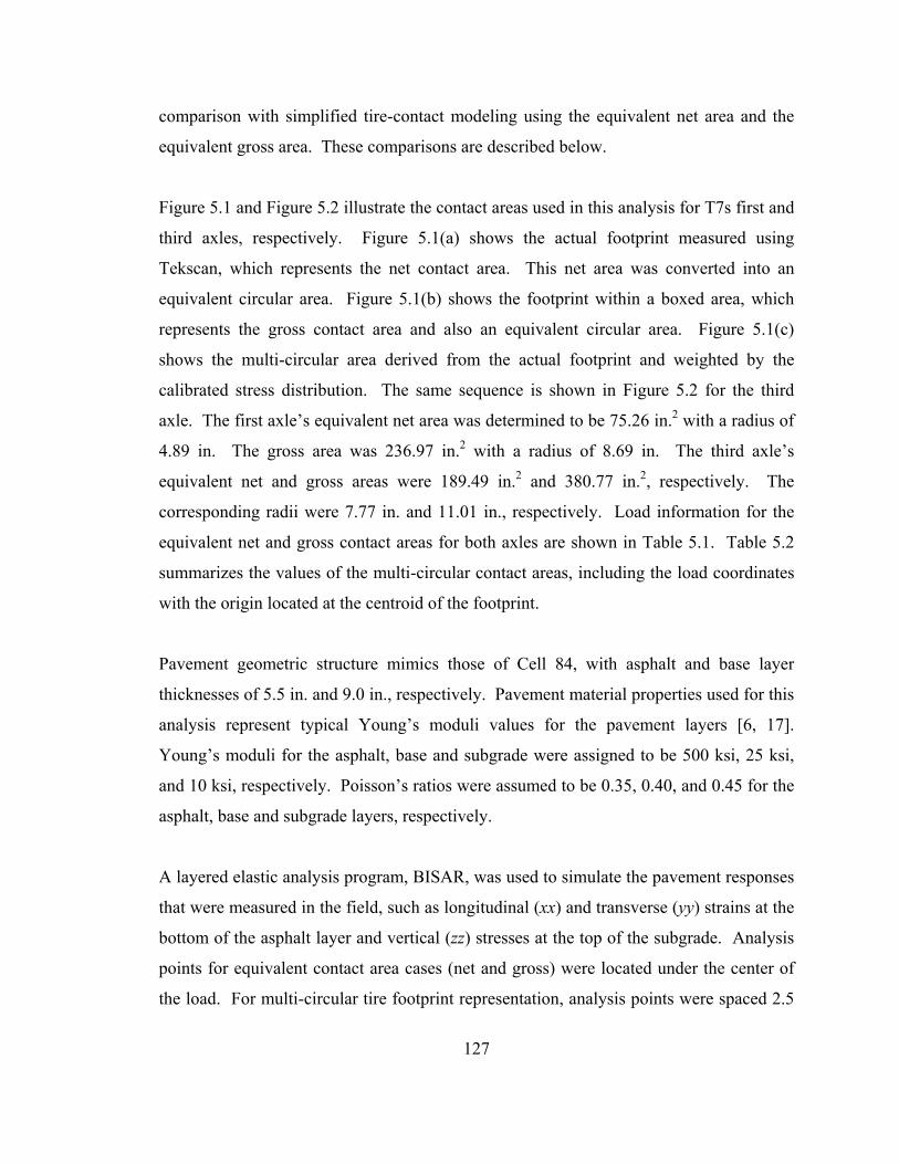
127

comparison with simplified tire-contact modeling using the equivalent net area and the

equivalent gross area. These comparisons are described below.

Figure 5.1 and Figure 5.2 illustrate the contact areas used in this analysis for T7s first and

third axles, respectively. Figure 5.1(a) shows the actual footprint measured using

Tekscan, which represents the net contact area. This net area was converted into an

equivalent circular area. Figure 5.1(b) shows the footprint within a boxed area, which

represents the gross contact area and also an equivalent circular area. Figure 5.1(c)

shows the multi-circular area derived from the actual footprint and weighted by the

calibrated stress distribution. The same sequence is shown in Figure 5.2 for the third

axle. The first axle’s equivalent net area was determined to be 75.26 in.2 with a radius of

4.89 in. The gross area was 236.97 in.2 with a radius of 8.69 in. The third axle’s

equivalent net and gross areas were 189.49 in.2 and 380.77 in.2, respectively. The

corresponding radii were 7.77 in. and 11.01 in., respectively. Load information for the

equivalent net and gross contact areas for both axles are shown in Table 5.1. Table 5.2

summarizes the values of the multi-circular contact areas, including the load coordinates

with the origin located at the centroid of the footprint.

Pavement geometric structure mimics those of Cell 84, with asphalt and base layer

thicknesses of 5.5 in. and 9.0 in., respectively. Pavement material properties used for this

analysis represent typical Young’s moduli values for the pavement layers [6, 17].

Young’s moduli for the asphalt, base and subgrade were assigned to be 500 ksi, 25 ksi,

and 10 ksi, respectively. Poisson’s ratios were assumed to be 0.35, 0.40, and 0.45 for the

asphalt, base and subgrade layers, respectively.

A layered elastic analysis program, BISAR, was used to simulate the pavement responses

that were measured in the field, such as longitudinal (xx) and transverse (yy) strains at the

bottom of the asphalt layer and vertical (zz) stresses at the top of the subgrade. Analysis

points for equivalent contact area cases (net and gross) were located under the center of

the load. For multi-circular tire footprint representation, analysis points were spaced 2.5

128

in. apart in both the x and y directions. A grid over the evaluation points from -7.5 in. to

7.5 in. in both the x and y directions was used in the analysis of the first axle. A grid over

the evaluation points from -7.5 in. to 7.5 in. in the x direction and -7.5 in. to 10 in. in the y

direction was used in the analysis of the third axle. Additional analysis points were

placed directly under each circle of the multi-circular loads for both axle cases.

(a)

(b)

(c) Figure 5.1. Vehicle T7’s first axle footprint modeling using (a) equivalent net contact

area (b) equivalent gross contact area (c) multi-circular area representation

129

(a)

(b)

(c)

Figure 5.2. Vehicle T7’s third axle footprint modeling using (a) equivalent net contact

area (b) equivalent gross contact area (c) multi-circular area representation

130

Table 5.1. Equivalent net and gross contact areas for vehicle T7

Area Radius Load Stress Axle Area [in.2] [in.] [lb] [psi]

Axle 1 Net 75.26 4.89 4860 64.58 Axle 1 Gross 236.97 8.69 4860 20.51 Axle 3 Net 189.49 7.77 8780 46.34 Axle 3 Gross 380.77 11.01 8780 23.06

Table 5.2. Multi-circular area representation values for vehicle T7’s first and third axle

x-coord y-coord Area Radius Load StressAxle Section [in.] [in.] [in.2] [in.] [lb] [psi]

1 -6.10 1.99 5.38 1.31 347.13 64.58 2 -5.21 -3.28 8.06 1.60 520.70 64.58 3 -1.83 5.40 9.41 1.73 607.48 64.58 4 -2.88 -1.33 7.17 1.51 462.84 64.58 5 1.03 2.11 8.06 1.60 520.70 64.58 6 1.07 -5.28 15.23 2.20 983.54 64.58 7 5.80 5.19 11.20 1.89 723.19 64.58

Axle 1

8 4.26 -1.89 10.75 1.85 694.27 64.58 1 -3.64 8.11 14.78 2.17 684.96 46.34 2 -3.97 0.12 34.49 3.31 1598.25 46.34 3 -5.06 -5.00 7.62 1.56 352.86 46.34 4 0.94 8.53 23.29 2.72 1079.34 46.34 5 0.98 -0.26 24.19 2.77 1120.85 46.34 6 -1.19 -6.27 28.67 3.02 1328.42 46.34 7 5.29 8.61 22.85 2.70 1058.58 46.34 8 6.38 0.54 21.05 2.59 975.56 46.34

Axle 3

9 4.17 -6.16 12.54 2.00 581.18 46.34

Table 5.3. Maximum computed responses for vehicle T7’s first and third axle

Longitudinal AC Strain (xx)

Transverse AC Strain (yy)

Vertical Subgrade Stress

(zz) Axle Area

[×10-6] [×10-6] [psi] Net 154 154 3.27

Gross 90 90 2.95 Axle 1 Multi-circular 100 97 3.01

Net 184 184 5.49 Gross 122 122 4.91 Axle 3

Multi-circular 163 139 5.10

131

Results of the layered elastic analysis are shown in Table 5.3. As expected, strain and

stress responses computed using equivalent net contact area were larger than those

calculated using the equivalent gross contact area. These discrepancies were more

profound for asphalt strains than subgrade stresses. This can be explained by the

complexity of the tire footprint and how it affects near surface responses. As the analysis

point moves away from the applied load, the effects of the load distribution geometry

(footprint) are less significant. One of the benefits of modeling using both net and gross

contact areas is the ability to establish a lower and upper limit in computed responses.

However, multi-circular representation of the tire contact generally provides a more

accurate and realistic representation of the vehicle load distribution and improved the

accuracy in response prediction. This proves to be an important aspect to be considered,

especially when it comes to simulating responses as a function of traffic wander.

5.3 Traffic Wander Simulation

To further evaluate the importance of vehicle traffic wander, a layered elastic simulation

using BISAR was performed for a footprint belonging to the third axle of vehicle T7

using the multi-circular footprint estimation as previously mentioned. This analysis was

performed to show that changes in the lateral direction of the wheel load would affect the

resulting strain at the bottom of the asphalt layer and stress on top of the subgrade. The

simulated pavement structure mimics the pavement section of Cell 84, with details shown

in Table 5.4. Figure 5.2(c) shows the footprint obtained using Tekscan and

corresponding multi-circular footprint estimation used for the layered elastic analysis.

Evaluation points were situated along the lateral direction from the center of the load to

simulate various vehicle offsets.

To validate the field observation that traffic wander influences pavement responses,

simulated asphalt strains and subgrade stresses were compared to the measurements

obtained from the field. Pavement responses generated by vehicle T7’s third axle were

examined. To eliminate the effects of layer material properties and focus on the effects

132

of traffic wander on pavement responses, the simulated longitudinal and transverse

asphalt strains were normalized using their respective maximum simulated strain values.

This normalization was also performed for simulated subgrade stresses. In addition, field

measurements were also normalized to their respective maximum values. Figure 5.3

shows the resulting normalized measured and simulated transverse and longitudinal

asphalt strains, and Figure 5.4 shows the resulting normalized measured and simulated

vertical subgrade stresses.

Table 5.4. BISAR pavement structure input parameters

Layer Young’s Modulus Poisson’s Ratio Thickness 1. Asphalt 500,000 psi 0.35 5.50 in.

2. Base 15,000 psi 0.40 9.00 in. 3. Subgrade 7,000 psi 0.45

Normalized AC Strain

-0.5

0

0.5

1

1.5

-15 -10 -5 0 5 10 15 20 25

Axle 3 relative offset [in.]

Nor

mal

ized

stra

in [

]

Longitudinal (meas)Transverse (meas)Longitudinal (sim)Transverse (sim)

Figure 5.3. Normalized measured and simulated longitudinal and transverse asphalt

strains

133

Normalized Subgrade Stress

0

0.5

1

1.5

-15 -10 -5 0 5 10 15 20 25

Axle 3 relative offset [in.]

Norm

aliz

ed s

tress

[ ]

Vertical (meas)Vertical (sim)

Figure 5.4. Normalized measured and simulated vertical subgrade stress

Figure 5.3 and Figure 5.4 show an excellent agreement between measured and simulated

trends. Figure 5.3 shows that both measured and calculated strains significantly decrease

as the load moves away from the sensor. This trend is more pronounced for the

transverse strains as compared to longitudinal strains, although it is still significant for the

longitudinal strains. For example, deviation of the footprint more than 15 in. from the

sensor caused a reduction in longitudinal strains by more than half. For the same

deviation from the sensor, the transverse strain changes from tension to compression.

Similar trends can be observed in Figure 5.4 for subgrade stresses. For example,

deviation of the footprint more than 15 in. from the sensor caused a reduction in subgrade

stresses by half. This analysis shows that field measurements and theoretical predictions

agree that the applied load position has a profound effect on pavement responses.

134

5.4 Backcalculation Analysis

Elastic properties in the pavement layer are important parameters for layered elastic

analysis. These parameters are usually determined either from laboratory studies or

FWD testing. Although these methods are widely accepted in pavement modeling, it is

desirable to check if the parameters can be obtained from measured stresses and strains.

In this study, a numerical optimization framework was developed to perform a

backcalculation analysis to obtain the layers’ Young’s moduli by matching the measured

pavement responses. This process utilizes two programs: the layered elastic software

called MnLayer and the optimization software called DAKOTA.

DAKOTA, developed by Sandia National Laboratories, is an abbreviation for Design

Analysis Kit for Optimization and Terascale Applications which main purpose is to

function as a toolkit for optimization methods, parameter estimation, and uncertainty

quantification, among others. The application of DAKOTA requires a user defined

simulation code, evaluation of the performance objectives, and parameter/variable

adjustment commands. Coupling together these items creates an iterative optimization

environment that outputs an optimal solution as defined in the performance objectives

[18]. In the case of the backcalculation optimization process employed here, the

simulation code is the layered elastic software MnLayer, the performance objective or

cost function is the error between computed and measured data, and the parameters are

the Young’s moduli values of the pavement layers. Figure 5.5 shows a flow chart

illustrating the overall schematic of the optimization process.

135

Figure 5.5. Flow chart of the optimization process

The general objective of this optimization process is to determine the Young’s moduli for

the asphalt, base, and subgrade layers denoted as E1, E2, and E3, respectively. This is

done by minimizing discrepancies between measurements obtained in the field generated

by a particular vehicle pass and corresponding responses predicted by MnLayer. The

process begins with assignment of an initial value for each layer moduli defined in the

DAKOTA input file. Next, the analysis driver transfers the moduli values into the

MnLayer input file via user defined scripts. The layered elastic analysis is then

performed to calculate stress on the top of the subgrade and strain at the bottom of the

asphalt layer. The maximum calculated stress and strain values are then extracted and

compared to the field measured stress and strain to obtain the cost function, e, expressed

in Eqn 5.1 also through a user defined script.

22

11 ⎟⎟⎠

⎞⎜⎜⎝

⎛−+⎟⎟

⎠

⎞⎜⎜⎝

⎛−=

meas

calc

meas

calceσσ

εε

Eqn 5.1

where e is the cost function

calcε is the calculated strain

measε is the measured strain

calcσ is the calculated stress

measσ is the measured stress

DAKOTA

MnLayer

Analysis Driver

Cost Function

136

After the cost function, e, is computed, it is returned to DAKOTA, which determines a

new set of values for E1, E2, and E3. The iteration continues until an acceptable cost

function is reached or until the maximum number of iterations is met. The optimization

method DAKOTA employs is in the COLINY (Common Optimization Library Interface)

library, which contains nongradient-based optimization algorithms suited for this exercise

[18]. In the COLINY library, a local optimization method is used, known as the pattern

search. The COLINY optimization method also supports upper and lower limits, as well

as nonlinear constraints imposed on the parameters. An example of the iteration process

was performed for the rear tandem axles (axles 4 and 5) of vehicle Mn80 at -2.5 in.

offset. This example used the measured asphalt strain and subgrade stress values of 426

×10-6 and 12.21 psi, respectively. Figure 5.6 through Figure 5.8 show an example of the

iteration process for E1, E2, and E3, while Figure 5.9 shows the convergence of the cost

function, e. The figures show the convergence pattern for each of the moduli values and

the cost function using the pattern search optimization method. According to Figure 5.9,

the minimum cost function, e was obtained at iteration number 163 with a value of 1.24

×10-9. Analysis of Figure 5.6 through Figure 5.8 showed that the Young’s moduli for the

asphalt (E1), base (E2), and subgrade (E3) layers converged to 565,844 psi, 8,054 psi,

and 6,274 psi, respectively at iteration number 163.

Asphalt Layer Young's Modulus, E 1

0

200

400

600

800

1000

0 50 100 150 200 250

Iteration number

Youn

g's

mod

ulus

[×10

3 psi

]

Figure 5.6. Convergence pattern for asphalt layer Young’s modulus, E1

137

Base Layer Young's Modulus, E 2

0

5

10

15

20

25

0 50 100 150 200 250

Iteration number

You

ng's

mod

ulus

[×10

3 psi

]

Figure 5.7. Convergence pattern for base layer Young’s modulus, E2

Subgrade Layer Young's Modulus, E 3

0

5

10

15

20

25

0 50 100 150 200 250

Iteration number

Youn

g's

mod

ulus

[×10

3 psi

]

Figure 5.8. Convergence pattern for subgrade layer Young’s modulus, E3

138

Cost Function, e

05

10152025303540

0 50 100 150 200 250

Iteration number

Cost

func

tion,

e [

]

Figure 5.9. Convergence pattern for cost function, e

5.4.1 Backcalculation through Vehicle Loading

An example of the DAKOTA-MnLayer backcalculation optimization process is

presented here to introduce the initial capabilities of this framework. A preliminary

backcalculation was performed based on seasonal changes to observe how moduli values

were affected. Responses collected for the trailers’ tandem axle of vehicle Mn80 (axles 4

and 5) were extracted and the maximum axle responses between axles 4 and 5 were used

as the variables to evaluate e. These axles were chosen because they represent the

heaviest axles of the vehicle. The upper and lower bounds of the optimized parameters

(i.e. E1, E2, and E3) were adjusted based on typical moduli ranges found in the literature

for different seasons. The Young’s modulus for the asphalt layer, E1, was assumed to be

generally lower in the fall compared to the spring season. The modulus for the subgrade,

E3, was assumed to be very stiff in spring due to its frozen state. Poisson’s ratio, ν, for

the asphalt, base, and subgrade layers were set at 0.35, 0.40, and 0.45, respectively.

Pavement geometric structure of Cell 84 was analyzed. Additionally, a constraint was

imposed such that parameter E2 could not be less than E3 for simulations performed for

the fall season. However, in the spring season the constraint was removed. Table 5.5

139

summarizes the initial values, upper bounds, and lower bounds used for this process.

Evaluation of measured vertical subgrade stress and longitudinal asphalt strain responses

generated by vehicle Mn80s’ axles 4 and 5 at Cell 84 for spring and fall seasons are

shown in Table 5.6.

Young’s moduli for the pavement layers are affected by the surrounding climatic

environment. The backcalculation analysis was performed under the presumption that

effect of temperature and moisture on pavement responses can be reflected by the

stiffness (moduli) of the pavement layers. According to Table 5.7, backcalculated moduli

within the specified bounds were deemed to be valid, since they produced cost functions

that were very close to zero. This further solidifies the assumptions previously made,

where the asphalt moduli are lower in fall than in spring and that the subgrade layer was

very stiff in spring. A forward analysis was later performed using the backcalculated

moduli values to check the accuracy of the optimization. This was achieved by

regenerating asphalt strains and subgrade stresses for vehicle Mn80s’ rear tandem axles

under the same conditions as the backcalculation. Table 5.8 shows the measured and

simulated asphalt strains and subgrade stresses for both the fall and spring seasons. The

forward analysis results proved to be satisfactory.

Table 5.5. Parameter initial values, upper, and lower bounds

Fall Season* E1 [ksi] E2 [ksi] E3 [ksi] Initial Value 30 12 12 Lower Bound 15 5 5 Upper Bound 500 50 50

Spring Season** E1 [ksi] E2 [ksi] E3 [ksi] Initial Value 500 12 250 Lower Bound 250 1 150 Upper Bound 2,000 50 300

*Contraint E2 ≥ E3 ** No constraint

140

Table 5.6. Response measurement variables for spring and fall seasons at Cell 84

RelativeOffset

Longitudinal AC Strain (xx)

Vertical Subgrade Stress (zz) Season Axle

[in.] [×10-6] [psi] Axle 4 -3.5 434 11.13 Fall Axle 5 -3.5 377 9.15 Axle 4 -3.0 133 9.75 Spring Axle 5 -3.0 136 9.81

Table 5.7. Backcalculated Young’s modulus values

Season E1 [ksi] E2 [ksi] E3 [ksi] e [ ] Fall 66.4 25.4 24.6 9.5 ×10-10

Spring 715.2 17.5 273.6 3.9 ×10-7

Table 5.8. Forward analysis using backcalculated moduli

Longitudinal AC Strain (xx) [×10-6]

Vertical Subgrade Stress (zz) [psi] Season

Relative Offset [in.] Measured Simulated Measured Simulated

Fall -3.5 434 434 11.13 11.13 Spring -3.0 136 136 9.81 9.81

5.4.2 Backcalculation through FWD Loading

Another example used to demonstrate the DAKOTA-MnLayer framework is shown in

this section with a comparison of backcalculated moduli using combinations of pavement

surface deflections, horizontal strain at the bottom of the asphalt layer, and vertical

subgrade stress measurements. Asphalt strain and subgrade stress responses generated by

dropping the falling weight deflectometer (FWD) load directly on top of the marked

sensor location were measured. In addition, the pavement deflection basin was measured

by the FWD device itself at 0, 8, 12, 18, 24, and 36 in. from the center of the load. Loads

applied by the FWD were 13 kip over an area with a radius 5.9 in. The FWD testing was

performed in July and September of 2010. Therefore, the parameter upper and lower

bounds were changed accordingly to address the constraint where E2 could not be less

141

than E3. The backcalculation of the layer moduli were conducted to match the following

measured responses:

• surface deflections only (case iδ )

• subgrade stress and surface deflections (case σ - iδ )

• asphalt strain and surface deflections (case ε - iδ )

• subgrade stress and asphalt strain (case σ -ε )

• surface deflections and asphalt strain and subgrade stress (case iδ -ε -σ )

In order to accommodate the additional variables to be evaluated in the optimization

process, computation of the cost function, e, was modified as shown by Eqn 5.2. This

modified e allows for the inclusion or exclusion of certain variables by changing the

weight factor, w. If a variable was considered in analysis than the corresponding weight

factor was set to be 1 whereas excluded variables had a weight factor of 0.

( ) ( ) ( )∑=

+⎟⎟⎠

⎞⎜⎜⎝

⎛−+⎟⎟

⎠

⎞⎜⎜⎝

⎛−+⎟⎟

⎠

⎞⎜⎜⎝

⎛−=

6

12

2

2

2

1

2

111i

iimeas

icalc

meas

calc

meas

calc wwweδδ

σσ

εε

Eqn 5.2

where e is the cost function

calcε is the calculated strain

measε is the measured strain

calcσ is the calculated stress

measσ is the measured stress

icalcδ is the ith calculated deflection

imeasδ is the ith measured deflection

w is the weight factor (either 0 or 1)

i is the number of deflection points (from 1 to 6 in this case)

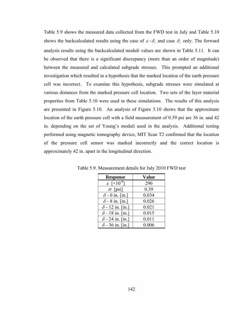
142

Table 5.9 shows the measured data collected from the FWD test in July and Table 5.10

shows the backcalculated results using the case of ε - iδ and case iδ only. The forward

analysis results using the backcalculated moduli values are shown in Table 5.11. It can

be observed that there is a significant discrepancy (more than an order of magnitude)

between the measured and calculated subgrade stresses. This prompted an additional

investigation which resulted in a hypothesis that the marked location of the earth pressure

cell was incorrect. To examine this hypothesis, subgrade stresses were simulated at

various distances from the marked pressure cell location. Two sets of the layer material

properties from Table 5.10 were used in these simulations. The results of this analysis

are presented in Figure 5.10. An analysis of Figure 5.10 shows that the approximate

location of the earth pressure cell with a field measurement of 0.39 psi are 36 in. and 42

in. depending on the set of Young’s moduli used in the analysis. Additional testing

performed using magnetic tomography device, MIT Scan T2 confirmed that the location

of the pressure cell sensor was marked incorrectly and the correct location is

approximately 42 in. apart in the longitudinal direction.

Table 5.9. Measurement details for July 2010 FWD test

Response Value ε [×10-6] 290 σ [psi] 0.39

δ - 0 in. [in.] 0.034 δ - 8 in. [in.] 0.026 δ - 12 in. [in.] 0.021 δ - 18 in. [in.] 0.015 δ - 24 in. [in.] 0.011 δ - 36 in. [in.] 0.006

143

Table 5.10. Backcalculated Young’s moduli values for July 2010 FWD test

Case E1 [ksi] E2 [ksi] E3 [ksi] e [ ] iδ only 229.4 14.5 14.5 9.0 ×10-3

ε - iδ 632.0 14.1 14.1 1.5 ×10-1

Table 5.11. Forward analysis results for two cases: iδ only and ε - iδ

Case iδ only Case ε - iδ Response Value Value

ε [×10-6] 636 333 σ [psi] 13.68 9.37

δ - 0 in. [in.] 0.035 0.026 δ - 8 in. [in.] 0.026 0.022 δ - 12 in. [in.] 0.021 0.019 δ - 18 in. [in.] 0.015 0.015 δ - 24 in. [in.] 0.011 0.011 δ - 36 in. [in.] 0.007 0.007

Subgrade Stress

0

0.4

0.8

1.2

1.6

2

0 10 20 30 40 50

Distance [in.]

Stre

ss [p

si]

case δcase ε-δ

Figure 5.10. Simulated subgrade stresses at varying locations for cases ε - iδ and iδ

Additional FWD testing was conducted in September 2010 using the confirmed sensor

location. The measured data as well as the results of the backcalculation analysis are

summarized in Table 5.12 and Table 5.13, respectively. To evaluate the accuracy of

these moduli, a forward analysis using the backalculated moduli was conducted for the

144

same FWD load to regenerate the asphalt strain and subgrade stress. The results of the

forward analysis are shown in Table 5.14. Due to the axisymmetric nature of the layered

elastic theory, asphalt strains directly beneath the center of the load are the same in both

longitudinal and transverse directions. These newly computed strains and stresses were

compared to the actual field responses and the error was computed using Eqn 5.1.

Table 5.12. Measurement details for September 2010 FWD test

Response Value ε [×10-6] 219 σ [psi] 7.06

δ - 0 in. [in.] 0.027 δ - 8 in. [in.] 0.023 δ - 12 in. [in.] 0.019 δ - 18 in. [in.] 0.015 δ - 24 in. [in.] 0.011 δ - 36 in. [in.] 0.006

Table 5.13. Backcalculated Young’s moduli values for September 2010 FWD test

Case E1 [ksi] E2 [ksi] E3 [ksi] e [ ] iδ only 401.8 15.2 15.2 1.2 ×10-2

σ - iδ 858.1 14.2 14.2 1.2 ×10-1

ε - iδ 961.4 14.2 14.2 1.3 ×10-1

σ -ε 1001.9 27.5 11.8 2.8 ×10-9

iδ -ε -σ 1019.0 14.2 14.2 1.4 ×10-1

Table 5.14. Forward analysis using backcalculated moduli

Case Asphalt Strain [×10-6] Subgrade Stress [psi] Error [ ]iδ only 445 11.58 1.5 σ - iδ 269 8.36 8.6 ×10-2

ε - iδ 248 7.97 3.4 ×10-2

σ -ε 219 7.06 8.0 ×10-7

iδ -ε -σ 238 7.76 1.7 ×10-2

145

As expected, the case where σ -ε are used in the DAKOTA-MnLayer optimization

process yielded the best results with the lowest error amongst all cases since it was

optimized to match the same values. Case iδ -ε -σ produced the second lowest error

followed by case ε - iδ , case σ - iδ , and finally case iδ only. When using deflection data

only, both asphalt strain and subgrade stress are overestimated. It is interesting to note

that the use of the deflection data in determination of Young’s moduli parameters leads to

an overestimation of the asphalt strains in the subsequent forward analysis. This suggests

that there is a possibility of incorrect sensor depth location. The analysis suggests that

the sensor is located at the bottom of the asphalt layer that may cause over-predictions of

the asphalt strains. This hypothesis should be further investigated in future field testing

and verified with coring. Another observation is that combining the deflection data with

strain and/or stress responses proved to be helpful in the backcalculation process.

The measurements obtained from the FWD testing conducted in September 2010 were

also used to verify the gage factor settings of the strain gages installed at the flexible

pavement test sections. As mentioned in Chapter 2, throughout this study, the strain gage

factor of two (GF2) was used as per manufacturer’s recommendation. Since strain is a

direct derivative of displacement, backcalculated Young’s moduli for the asphalt layer,

E1, using cases ε - iδ and iδ only should result in comparable values. However, this was

not observed in Table 5.13 with E1 for case iδ only being 41% of E1 for case ε - iδ .

This led to a presumption that the strain gages might be incorrectly calibrated. MnROAD

personnel currently suggest the use of gage factor one (GF1), which multiplies the current

strain values by two. Backcalculation was performed to compare the Young’s moduli of

the pavement layers obtained using measured strains adjusted for GF1. Measurements

from Table 5.12 were used for this analysis where the strain value using GF1 was 438

×10-6. A change in the strain value affected cases σ -ε , ε - iδ , and iδ -ε -σ , therefore,

only these cases were evaluated. Table 5.15 summarizes the backcalculated Young’s

moduli for this comparison. The backcalculated moduli values were then used to perform

a forward analysis to simulate subgrade stresses and asphalt strains for each of the cases

146

as shown in Table 5.16. Eqn 5.1 was used to compute the error between the simulated

and measured responses corresponding to the respective measured strain values for GF1

and GF2.

Table 5.15. Comparison of backcalculated Young’s moduli between GF1 and GF2

Gage Factor Case E1 [ksi] E2 [ksi] E3 [ksi] e [ ] iδ only 401.8 15.2 15.2 1.2 ×10-2

NA σ - iδ 858.1 14.2 14.2 1.2 ×10-1

ε - iδ 961.4 14.2 14.2 1.3 ×10-1

σ -ε 1001.9 27.5 11.8 2.8 ×10-9 GF2 iδ -ε -σ 1019.0 14.2 14.2 1.4 ×10-1

ε - iδ 407.5 15.4 15.4 1.9 ×10-2 σ -ε 565.8 8.1 6.3 1.2 ×10-9 GF1 iδ -ε -σ 645.2 14.2 14.2 2.3 ×10-1

Table 5.16. Forward analysis using backcalculated moduli for GF1 and GF2

Gage Factor Case

Asphalt Strain [×10-6]

Subgrade Stress [psi]

GF2 Error [ ]

GF1 Error [ ]

iδ only 445 11.58 1.5 4.1 ×10-1 NA

σ - iδ 269 8.36 8.6 ×10-2 1.8 ×10-1 ε - iδ 248 7.97 3.4 ×10-2

σ -ε 219 7.06 8.0 ×10-7 GF2 iδ -ε -σ 238 7.76 1.7 ×10-2

NA

ε - iδ 439 11.56 4.1 ×10-1 σ -ε 438 7.06 3.6 ×10-9 GF1 iδ -ε -σ 330 9.41

NA 1.7 ×10-1

The value for E1 backcalculated from case iδ only was 401.8 ksi. This value was used

as a benchmark to evaluate the difference between cases of GF2 and GF1. Referring to

case ε - iδ for GF1 and GF2, it was found that GF1 resulted in a more comparable E1

value at 407.5 ksi while E1 for GF2 was 961.4 ksi. Recall that the measured subgrade

stress was 7.06 psi and the measured strain for GF2 was 219 ×10-6. The adjusted

147

measured strain for GF1 was 438 ×10-6. Table 5.16 shows that the simulated strains for

case ε - iδ of GF1 and GF2 match reasonably well with their corresponding measured

strains. However, simulated strain for case ε - iδ of GF1 was closer to the strain

simulated through case iδ only. On the other hand, simulated stresses for case ε - iδ of

GF1 and GF2 were larger than the measured stress at approximately 60% and 13%,

respectively. Asphalt strain which was corrected using GF1 yielded results that were

more comparable to the deflection data (case iδ only) measured from the FWD testing.

However, a forward analysis using backcalculated Young’s moduli for GF1 greatly

overestimates subgrade stresses whereas backcalculated moduli for GF2 resulted in more

favorable simulated stresses. This analysis is currently inconclusive and an in-depth

investigation should be performed by calibrating the strain gages with a known

displacement.

5.5 Summary

The purpose of this section was to introduce a preliminary mechanistic model aiming to

verify the trends observed in field testing as well as identify the material parameters that

can be used for future structural modeling of pavement responses from agricultural

vehicles. The layered elastic analysis programs, MnLayer and BISAR were used in the

analysis. The importance of detailed modeling of the tire footprint was demonstrated.

The layered elastic analysis also confirmed the field-observed effect of traffic wander.

The optimization program DAKOTA was combined with MnLayer for material

characterization. It was shown that the combination of MnLayer and DAKOTA provide

a capability to determine the material parameters that lead to a close match between the

predicted and measured pavement responses. This framework was also useful for

verification of the location of the sensors and strain gage factor settings.

148

Chapter 6 Conclusions

Agricultural equipment manufacturers have been producing equipment with larger

capacity to meet the demands of the agricultural industry. Agricultural vehicles today are

equipped with innovations such as improved tire designs, flotation tires, and steerable

axles. However, equipments with larger capacities result in heavier vehicle axle weights.

This causes concerns to pavement owners because the potential for pavement damage in

public highways and local roads increase due to heavy vehicle loading. This study was

initiated to investigate the validity of these concerns. Full scale accelerated pavement

testing was conducted at the MnROAD test facility to determine pavement responses

generated by heavy agricultural equipment loading. These responses were compared to a

typical 5-axle 80-kip semi truck.

Both flexible and rigid pavements were tested in this study. This thesis presented

analysis for the flexible pavement sections. Cell 83 represented a thinner pavement rated

as a 7-ton road while Cell 84 represented a thicker pavement rated as a 10-ton road. Both

sections were instrumented with strain gages, LVDTs, earth pressure cells, and

thermocouples. Testing was conducted twice a year: once in the month of March and

once in the month of August. A total of twelve agricultural vehicles were tested together

with two 5-axle semi trucks designated as control vehicles.

Preliminary data analysis of the collected data was performed and numerous effects on

pavement responses were identified. These effects ranged from traffic wander to time of

testing. The following summarizes the findings of this study:

• The lateral position of the vehicle’s wheel path or traffic wander relative to the

sensor location had a profound effect on the measured responses. Actual

measurements of the vehicle traffic wander provided pavement response

distribution across the pavement width relative to the sensor location. Maximum

149

responses may be generated by different vehicle axles depending on response

type, load level, and axle configuration.

• Effects of seasonal changes were observed through analysis performed on

pavement responses from the standard Mn80 truck. Measured asphalt strains in

fall seasons were larger than those measured in the spring due to the less stiff

asphalt layer. This trend was not observed for subgrade stresses.

• Analysis of response variation within each day showed that both asphalt strains

and subgrade stresses measured in the morning were lower than those measured

in the afternoon for all vehicles during spring and fall seasons. Additionally,

there were no signs of distress propagation in the morning sessions while visible

damage was observed in some of the afternoon sessions.

• A thicker pavement structure resulted in lower asphalt strains and subgrade

stresses. As the vehicle moved toward the pavement edge, measured pavement

responses decreased significantly with the presence of a paved shoulder. An

unpaved (aggregate) shoulder provided little support at the pavement edge

resulting in the lack of any decrease in pavement responses as the vehicle moved

toward the shoulder.

• An increase in gross vehicle weight did not lead to a proportional increase in

individual axle weights. It was observed that an increase in gross vehicle weight

resulted in an increase in both asphalt strain and subgrade stress responses,

although not proportionally to the gross weight increase. Adding more axles to

the equipments’ tanker successfully reduced axle weights. It was also observed

that subgrade stresses increase linearly with individual axle weight but this trend

was not observed for asphalt strains.

150

• All agricultural vehicles loaded above 80% load level generated higher subgrade

stresses compared to the standard Mn80 truck regardless of test season.

• Asphalt strains were lower for the Mn80 truck compared to the agricultural

vehicles loaded above 80% load level in the spring seasons. However, in the fall

seasons, asphalt strains were consistently higher for Mn80 compared to the other

vehicles. It should also be noted that at 80% load level, the weight of the

heaviest axle of all the agricultural vehicles was larger than the heaviest axle of

Mn80 except for vehicle T2.

• Benefits of flotation tires (on vehicle S5) over radial ply tires (on vehicle S4)

were not significant. Changes in contact area and average contact stress were

similar as axle weight increases for both tire types. The pavement responses

across the pavement width were slightly higher for vehicle S4 with radial tires.

• The effect of vehicle speed on pavement responses was not significant in this

study. This may be due to the narrow range of tested vehicle speeds (up to 25

mph).

• Layered elastic programs BISAR and MnLayer were used in the modeling

analysis. Pavement responses simulated using the equivalent net contact area

were larger than responses simulated for the gross contact area. Tekscan

measurements were used to obtain a multi-circular area estimation of the

vehicles’ footprint. This detailed modeling of the tire footprint yielded a more

realistic representation of the actual vehicle footprint.

• Using the multi-circular area estimation and BISAR, the effect of traffic wander

on pavement responses was reconfirmed.

151

• The DAKOTA-MnLayer optimization framework was introduced here to aid in

the backcalculation analysis to determine the Young’s moduli of the pavement

layers. This optimization framework was capable of determining pavement

material properties which resulted in a close match between predicted responses

and field measurements.

152

Bibliography

[1] Minnesota Department of Agriculture. (2010). Agriculture - The Foundation of Minnesota's Economy. Retrieved from http://www.mda.state.mn.us/news/publications/kids/maitc/agprofile.pdf.

[2] United States Department of Agriculture. (2009). 2007 Census of Agriculture. Retrieved from http://www.agcensus.usda.gov/Publications/2007/Full_Report/index.asp.

[3] Phares, B. M, Wipf, T., Ceylan, H. (2005). Impacts of Overweight Implements of Husbandry on Minnesota Roads and Bridges. Minnesota Department of Transportation, Synthesis Report MN/RC-2005-05, Minnesota.

[4] Oman, M., Deusen, D. V., Olson, R. (2001). Scoping Study: Impact of Agricultural Equipment on Minnesota's Low Volume Roads. Minnesota Department of Transportation, Final Report, Minnesota.

[5] Fanous, F., Coree, B., Wood, D. (1999). Response of Iowa Pavements to Heavy Agricultural Loads. Center for Transportation Research and Education at Iowa State University, Interim Report, Iowa.

[6] Fanous, F., Coree, B., Wood, D. (2000). Response of Iowa Pavements to a Tracked Agricultural Vehicle. Center for Transportation Research and Education at Iowa State University, Final Report, Iowa.

[7] Sebaaly, P. E., Siddharthan, R. V., El-Desouky, M., Pirathapan, Y., Hitti, E., Vivekanathan, Y. (2002). Effects of Off-Road Tires on Flexible and Granular Pavements. South Dakota Department of Transportation, Final Report SD1999-15-F, South Dakota

[8] Tekscan, Inc. (2007). I-Scan® User Manual v.5.9x. Massachusetts. [9] Clyne, T. (2009). Cell 83 Forensic. Minnesota Department of Transportation,

Report, Minnesota. [10] Srirangarajan, S., Tewfik, S. H. (2007). MnROAD Offline Data Peak-Picking

Program User Guide. Department of Electrical and Computer Engineering, University of Minnesota, Minnesota.

[11] Loulizi, A., Al-Qadi, I. L., Elseifi, M. (2006). Difference between In Situ Flexible Pavement Measured and Calculated Stresses and Strains. Journal of Transportation Engineering, 132(7), 574-579.

[12] Novak, M., Birgisson, B., Roque, R. (2003). Tire Contact Stresses and Their Effects on Instability Rutting of Asphalt Mixture Pavements. Transportation Research Record, 1853, 150-156

[13] Park, D., Fernando, E., Leidy, J. (2005). Evaluation of Predicted Pavement Response with Measured Tire Contact Stresses. Transportation Research Record, 1919, 160-170.

[14] Siddharthan, R. V., Sebaaly, P. E., El-Desouky, M., Strand, D., Huft, D. (2005). Heavy Off-Road Vehicle Tire-Pavement Interactions and Response. Journal of Transportation Engineering, 131(3), 239-247.

153

[15] Huang, Y. H. (2004). Pavement Analysis and Design (Second Edition). New Jersey, Pearson Prentice Hall.

[16] Al-Qadi, I. L., Yoo, P. J., Elseifi, M. A., Janajreh, I. (2005). Effects of Tire Configurations on Pavement Damage. Journal of the Association of Asphalt Paving Technologists, 74, 921-962.

[17] Sebaaly, P. E., Siddharthan, R. V., El-Desouky, M., Strand, D., Huft, D. (2003). Effect of Off-Road Equipment on Flexible Pavements. Transportation Research Record, 1821, 29-38.

[18] Sandia National Laboratories. (2010). DAKOTA, A Multilevel Parallel Object-Oriented Framework for Design Optimization, Parameter Estimation, Uncertainty Quantification, and Sensitivity Analysis Version 5.0 User’s Manual. California

[19] Willis, J. R., Timm, D. (2009). Repeatability of Asphalt Strain Measurements Under Falling Weight Deflectometer Loading. Transportation Research Record, 2094, 3-11.

[20] de Jong, D.L., Peutz, M.G. F., Korswagen, A.R. (1979) Computer Program BISAR, Layered Systems under Normal and Tangential Surface Loads. Koninklijke/Shell Laboratorium, Amsterdam.

[21] Khazanovich, L., Wang, Q. (2007). MnLayer High-Performance Layered Elastic Analysis Program. Transportation Research Record, 2037, 63-75.

[22] Willis, J. R. (2008). A Synthesis of Practical and Appropriate Instrumentation Use for Accelerated Pavement Testing in the United States. Proceedings, International Conference on Accelerated Pavement Testing 2008, Madrid, Spain.

[23] Theyse, H. L. (2002). Stiffness, Strength, and Performance of Unbound Aggregate Material: Application of South African HVS and Laboratory Results to California Flexible Pavements. University of California Pavement Research Center, Report, California.

[24] Von Quintus, H. L., Simpson, A. L. (2002). Back-Calculation of Layer Parameters for LTPP Test Sections, Volume II: Layered Elastic Analysis for Flexible and Rigid Pavements. Federal Highway Administration, Final Report FHWA-RD-01-113, Virginia.

[25] de Beer, M., Fisher, C., Jooste, F. (1997). Determination of Pneumatic Tyre/Pavement Interface Contact Stresses under Moving Loads and Some Effects on Pavements with Thin Asphalt Surfacing Layers. Proceedings, Eighth International Conference of Asphalt Pavements, Vol. 1, 179-226.

[26] Chadbourn, B. A., Newcomb, D. E., Timm, D. H. (1997). Measured and Theoretical Comparisons of Traffic Loads and Pavement Response Distributions. Proceedings, Eighth International Conference of Asphalt Pavements, Vol. 1, 229-238.

[27] Dai, S. T., Van Deusen, D., de Beer, M., Rettner, D., Cochran, G. (1997). Investigation of Flexible Pavement Response to Truck Speed and FWD Load Through Instrumented Pavements. Proceedings, Eighth International Conference of Asphalt Pavements, Vol. 1, 141-160.

[28] Weissman, S. L. (1999). Influence of Tire-Pavement Contact Stress Distribution on Development of Distress Mechanisms in Pavements. Transportation Research Record, 1655, 161-167.

154

[29] Gillespie, T. D., Karamihas, S. M., Cebon, D., Sayers, M. W., Nasim, M. A., Hansen, W., Ehsan, N. (1992). Effects of Heavy Vehicle Characteristics on Pavement Responses and Performance, National Cooperative Highway Research Program (NCHRP), Final Report UMTRI 92-2, Washington D.C.

[30] Gaurav, S., Wojtkiewicz, S., Khazanovich, L. (in-press). Optimal Design of Flexible Pavements using a Framework of DAKOTA and MEPDG. International Journal of Pavement Engineering.

[31] Moore, D. S., McCabe, G. P., Craig, B. A. (2009). Introduction to the Practice of Statistics (Sixth Edition). New York, W. H. Freeman and Company.

[32] Das, B. M. (2005). Fundamentals of Geotechnical Engineering (Second Edition). Ontario, Canada, Thomson Canada Limited.

[33] Chou, P. C., Pagano, N. J. (1992). Elasticity: Tensor, Dyadic, and Engineering Approaches. New York, Dover.

155

Appendix A Test Program Example

The following shows a portion of the test program used for Cell 83 on the 16 March 2009

test. Table A.1 shows the test program before the start of testing with the actual time,

strain gage filename and LVDT filename columns empty. The empty columns were

filled during the test as shown in Table A.2. It should be mentioned that the Megadec-

TCS filenames correspond to the data file collected for strain and stress measurements

and the NI filenames correspond to the displacement measurements.

156

Table A.1. Example of empty test program

Cell 83 Test # Actual Time Pass Vehicle Load Level [%] Speed [mph] Offset [in.] Megadec-TCS Filename NI Filename 1 1 S4 0 5 12 2 1 S5 0 5 12 3 1 T6 0 5 12 4 1 T7 0 5 12 5 1 T8 0 5 12 6 1 Mn80 0 5 12 7 1 MN102 0 5 12 8 2 S4 0 5 0 9 2 S5 0 5 0

10 2 T6 0 5 0 11 2 T7 0 5 0 12 2 T8 0 5 0 13 2 Mn80 0 5 0 14 2 MN102 0 5 0 15 3 S4 0 10 0 16 3 S5 0 10 0 17 3 T6 0 10 0 18 3 T7 0 10 0 19 3 T8 0 10 0 20 3 Mn80 0 10 0 21 3 MN102 0 10 0

157

Table A.2. Example of filled test program

Cell 83 Test # Actual Time Pass Vehicle Load Level [%] Speed [mph] Offset [in.] Megadec-TCS Filename NI Filename 1 10:56 AM 1 S4 0 5 12 Cell 83 03-16-09 Set1_1_2 Cell 83 LVDT 3-16-09_0001 2 11:00 AM 1 S5 0 5 12 Cell 83 03-16-09 Set1_1_3 Cell 83 LVDT 3-16-09_0002 3 11:01 AM 1 T6 0 5 12 Cell 83 03-16-09 Set1_1_4 Cell 83 LVDT 3-16-09_0003 4 11:03 AM 1 T7 0 5 12 Cell 83 03-16-09 Set1_1_5 Cell 83 LVDT 3-16-09_0004 5 11:06 AM 1 T8 0 5 12 Cell 83 03-16-09 Set1_1_6 Cell 83 LVDT 3-16-09_0005 6 11:08 AM 1 Mn80 0 5 12 Cell 83 03-16-09 Set1_1_7 Cell 83 LVDT 3-16-09_0006 7 11:09 AM 1 MN102 0 5 12 Cell 83 03-16-09 Set1_1_8 Cell 83 LVDT 3-16-09_0007 8 11:11 AM 2 S4 0 5 0 Cell 83 03-16-09 Set1_1_9 Cell 83 LVDT 3-16-09_0008 9 11:13 AM 2 S5 0 5 0 Cell 83 03-16-09 Set1_1_10 Cell 83 LVDT 3-16-09_0009

10 11:14 AM 2 T6 0 5 0 Cell 83 03-16-09 Set1_1_11 Cell 83 LVDT 3-16-09_0010 11 11:16 AM 2 T7 0 5 0 Cell 83 03-16-09 Set1_1_12 Cell 83 LVDT 3-16-09_0011 12 11:17 AM 2 T8 0 5 0 Cell 83 03-16-09 Set1_1_13 Cell 83 LVDT 3-16-09_0012 13 11:18 AM 2 Mn80 0 5 0 Cell 83 03-16-09 Set1_1_14 Cell 83 LVDT 3-16-09_0013 14 11:19 AM 2 MN102 0 5 0 Cell 83 03-16-09 Set1_1_15 Cell 83 LVDT 3-16-09_0014 15 11:20 AM 3 S4 0 10 0 Cell 83 03-16-09 Set1_1_16 Cell 83 LVDT 3-16-09_0015 16 11:21 AM 3 S5 0 10 0 Cell 83 03-16-09 Set1_1_17 Cell 83 LVDT 3-16-09_0016 17 11:22 AM 3 T6 0 10 0 Cell 83 03-16-09 Set1_1_18 Cell 83 LVDT 3-16-09_0017 18 11:23 AM 3 T7 0 10 0 Cell 83 03-16-09 Set1_1_19 Cell 83 LVDT 3-16-09_0018 19 11:24 AM 3 T8 0 10 0 Cell 83 03-16-09 Set1_1_20 Cell 83 LVDT 3-16-09_0019 20 11:25 AM 3 Mn80 0 10 0 Cell 83 03-16-09 Set1_1_21 Cell 83 LVDT 3-16-09_0020 21 11:25 AM 3 MN102 0 10 0 Cell 83 03-16-09 Set1_1_22 Cell 83 LVDT 3-16-09_0021

158

Appendix B Vehicle Axle Weight and Dimension

Vehicle axle weights are tabulated in this section for all tested load levels and test season.

All weights are measured and presented in pounds as shown in Table B.1 through Table

B.6. Consequently, the axle configurations and dimensions of tested vehicles are

presented as shown in Figure B.1 through Figure B.4. All dimensions were measured

and presented in inches.

159

Table B.1. Vehicle axle weights for spring 2008 test

Vehicle S4, Homemade, 4,400 gal S5, Homemade, 4,400 gal T1, John Deere 8430, 6,000 gal Load Level 0% 25% 50% 80% 0% 25% 50% 80% 0% 25% 50% 80%

Axle 1 10,440 11,600 12,560 13,540 12,700 14,180 15,700 17,520 12,940 12,360 11,440 11,080 Axle 2 7,700 11,000 15,060 19,320 8,320 12,120 15,740 19,760 17,300 19,220 23,000 24,560 Axle 3 6,820 11,200 15,540 20,240 7,080 10,860 15,150 19,900 6,280 11,540 16,760 21,000 Axle 4 7,980 13,440 19,550 24,680 Axle 5 Axle 6 Total 24,960 33,800 43,160 53,100 28,100 37,160 46,590 57,180 44,500 56,560 70,750 81,320

Vehicle S3, Terragator 8204 T2, M.Ferguson 8470, 4,000 gal T6, John Deere 8430, 6,000 gal Load Level 0% 25% 50% 80% 0% 25% 50% 80% 0% 25% 50% 80%

Axle 1 13,920 14,000 14,120 14,980 9,080 9,060 8,580 8,400 13,220 12,660 11,940 11,600 Axle 2 17,680 20,880 24,820 30,600 12,700 13,460 15,220 16,180 17,600 17,700 20,860 22,420 Axle 3 4,520 8,260 12,100 16,920 7,140 12,420 16,620 22,440 Axle 4 4,480 7,660 11,440 15,620 7,900 13,760 19,760 26,640 Axle 5 Axle 6 Total 31,600 34,880 38,940 45,580 30,780 38,440 47,340 57,120 45,860 56,540 69,180 83,100

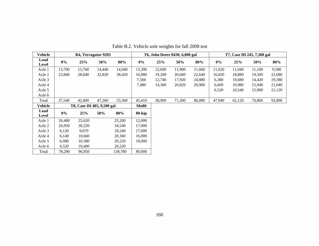
160

Table B.2. Vehicle axle weights for fall 2008 test

Vehicle R4, Terragator 9203 T6, John Deere 8430, 6,000 gal T7, Case IH 245, 7,300 gal Load Level 0% 25% 50% 80% 0% 25% 50% 80% 0% 25% 50% 80%

Axle 1 13,700 13,760 14,440 14,940 13,390 12,600 11,900 11,660 11,620 11,040 11,100 9,580 Axle 2 23,840 28,640 32,820 38,420 16,980 19,200 20,660 22,640 16,820 18,880 19,500 22,680 Axle 3 7,560 12,740 17,920 24,880 6,380 10,680 14,420 19,380 Axle 4 7,480 14,360 20,820 26,900 6,600 10,980 15,940 21,040 Axle 5 6,520 10,540 15,900 21,120 Axle 6 Total 37,540 42,400 47,260 53,360 45,410 58,900 71,300 86,080 47,940 62,120 76,860 93,800

Vehicle T8, Case IH 485, 9,500 gal Mn80 Load Level 0% 25% 50% 80% 80-kip

Axle 1 26,480 25,620 25,200 12,000 Axle 2 26,950 30,220 34,540 17,000 Axle 3 6,120 9,670 18,240 17,000 Axle 4 6,140 10,660 20,360 16,000 Axle 5 6,080 10,380 20,220 18,000 Axle 6 6,520 10,400 20,220 Total 78,290 96,950 138,780 80,000

161

Table B.3. Vehicle axle weights for spring 2009 test

Vehicle S4, Homemade, 4,400 gal S5, Homemade, 4,400 gal R4, Terragator 9203 Load Level 0% 25% 50% 80% 0% 25% 50% 80% 0% 25% 50% 80%

Axle 1 12,680 13,940 15,100 16,600 11,140 12,080 13,280 15,400 12,800 13,020 13,620 13,900 Axle 2 6,480 9,900 15,600 19,520 6,940 11,120 14,320 19,400 23,720 28,160 34,440 39,340 Axle 3 8,700 12,420 16,280 21,460 7,100 10,840 15,340 20,040 Axle 4 Axle 5 Axle 6 Total 27,860 36,260 46,980 57,580 25,180 34,040 42,940 54,840 36,520 41,180 48,060 53,240

Vehicle R5, Terragator 8144 T6, John Deere 8230, 6,000 gal T7, Case IH 335, 7,300 gal Load Level 0% 25% 50% 80% 0% 25% 50% 80% 0% 25% 50% 80%

Axle 1 15,240 15,580 16,260 16,780 7,900 7,500 7,240 6,320 13,880 13,760 11,820 17,240 Axle 2 16,240 19,940 23,340 26,960 15,860 17,720 19,140 20,960 19,020 20,440 23,080 18,360 Axle 3 7,140 12,160 17,460 20,480 8,520 12,680 17,680 22,840 Axle 4 7,880 13,240 19,400 22,460 8,440 12,780 17,540 22,720 Axle 5 8,680 13,180 17,930 22,440 Axle 6 Total 31,480 35,520 39,600 43,740 38,780 50,620 63,240 70,220 58,540 72,840 88,050 103,600

Vehicle T8, Case IH 335, 9,500 gal Mn80 Mn102 Load Level 0% 25% 50% 80% 80-kip 102-kip

Axle 1 17,400 17,800 17,240 15,540 11,640 12,880 Axle 2 18,060 21,480 22,260 26,040 17,080 22,180 Axle 3 5,660 9,700 14,540 18,760 16,760 21,540 Axle 4 6,100 10,500 16,200 21,280 18,460 22,680 Axle 5 5,720 10,240 16,060 20,840 15,620 22,960 Axle 6 5,960 10,620 15,780 21,380 Total 58,900 80,340 102,080 123,840 79,560 10,2240

162

Table B.4. Vehicle axle weights for fall 2009 test

Vehicle R5, Terragator 8144 T6, John Deere 8230, 6,000 gal T7, Case IH 275, 7,300 gal Load Level 0% 50% 100% 0% 50% 100% 0% 50% 100%

Axle 1 15,290 16,450 17,150 9,110 8,900 8,100 8,800 8,100 6,900 Axle 2 16,440 23,500 29,950 15,710 18,600 21,400 13,500 16,400 19,800 Axle 3 6,990 16,600 26,500 7,700 17,100 26,300 Axle 4 7,900 20,300 33,500 7,500 16,900 26,200 Axle 5 7,600 17,100 26,000 Axle 6 Total 31,730 39,950 47,100 39,710 64,400 89,500 45,100 75,600 105,200

Vehicle T8, Case IH 335, 9,500 gal Mn80 Mn102 Load Level 0% 50% 100% 80-kip 102-kip

Axle 1 16,800 16,100 14,800 12,100 12,780 Axle 2 18,000 21,000 25,200 17,440 24,440 Axle 3 5,900 14,900 23,300 16,050 20,780 Axle 4 5,900 15,100 23,700 18,830 24,330 Axle 5 5,700 15,100 23,500 16,670 22,910 Axle 6 5,900 15,400 23,700 Total 58,200 97,600 134,200 81,090 105,240

163

Table B.5. Vehicle axle weights for spring 2010 test

Vehicle R6, Terragator 3104 T6, John Deere 8230, 6,000 gal Mn80 Mn102 Load Level 0% 50% 100% 0% 50% 100% 80-kip 102-kip

Axle 1 24,150 28,300 32,800 8,200 7,500 6,200 12,550 12,200 Axle 2 17,900 28,700 41,900 17,600 21,000 23,500 16,000 22,950 Axle 3 7,200 16,900 26,000 17,800 22,250 Axle 4 8,000 21,400 33,900 16,000 20,700 Axle 5 17,800 25,000 Axle 6 Total 42,050 57,000 74,700 41,000 66,800 89,600 80,150 103,100

Table B.6. Vehicle axle weights for fall 2010 test

Vehicle G1, Case IH 9330, 1,000 bushels

T6, New Holland TG245, 6,000 gal Mn80 Mn102

Load Level 0% 100% 0% 100% 80-kip 102-kip

Axle 1 12,600 11,500 11,400 11,200 11,450 12,400 Axle 2 14,800 18,700 17,500 23,000 17,200 22,950 Axle 3 10,500 57,200 7,000 24,700 17,200 22,250 Axle 4 7,900 31,400 14,300 19,900 Axle 5 19,300 25,600 Axle 6 Total 37,900 87,400 43,800 90,300 79,450 103,100

164

S4 (Homemade 4,400 gal – radial tires) S5 (Homemade 4,400 gal – flotation tires) G1 (Case IH 9330, 1,000 bushels)

Figure B.1. Dimensions for vehicles S4, S5, and G1

19”50”

133”

120”

260”

90”83”

24”

80”

196”

52”

13”

8”

84”

74”

22”

56”

180”

12”

Forw

ard

165

R4 (AGCO Terragator 9203) R5 (AGCO Terragator 8144) R6 (ACGO Terragator 3104)

Figure B.2. Dimensions for vehicles R4, R5, and R6

83”

83”

38”

38”

226”

38”

93”

100”185”

27”

42”

95”

41”

267”

Forw

ard

166

T6 (John Deere 8203, 6,000 gal) T7 (Case IH 335, 7,300 gal) T8 (Case IH 335, 9,500 gal)

Figure B.3. Dimensions for vehicles T6, T7, and T8

104”

20”46” 99”

28”

127”

222”

68”

68”

68”

105”

17”

17”47” 95”

26”

120”

223”

70”

70”

14”

47”

30”

103”

90”

17” 64”121”

230”

72”

Forw

ard

167

Mn80 (Navistar 80-kip) Mn102 (Mack 102-kip)

Figure B.4. Dimensions for vehicles Mn80 and Mn102

26”

12”

12”

205” 81”

73”

26”

74”

12”

50”

50”

388”

25”

11”

11”

210” 80”

72”

25”

74”

11”

52”

48”

388”

Forw

ard

168

Appendix C Sensor Status

This section contains the status of sensors located at the flexible pavement sections. This

includes sensors from the Megadec-TCS and NI data acquisition systems. Sensor status

for all tested seasons for both Cells 83 and 84 are presented in Table C.1 and Table C.2,

respectively.

169

Table C.1. Sensor status for Cell 83

System Sensor Spring 2008 Fall 2008 Spring 2009 Fall 2009 Spring 2010 Fall 2010 83TE4 working working not working not working not working not working83TE5 working working working working not working not working83TE6 working not working not working not working not working not working83LE4 not working not working not working not working not working not working83LE5 working working working working working not working83LE6 not working not working working working working not working83AE4 working working working working not working not working83AE5 not working not working not working not working not working not working83AE6 working working working working working not working83PG4 working working working working not working not working83PG5 working working working working not working not working

Meg

adec

-TC

S

83PG6 working working working working not working not working83AL1 not working working working not working not working not working83AH2 not working working working not working not working not workingN

I

83AV3 not working working working not working not working not working

170

Table C.2. Sensor status for Cell 84

System Sensor Spring 2008 Fall 2008 Spring 2009 Fall 2009 Spring 2010 Fall 2010 84TE4 working working working working working working 84TE5 working working working working working working 84TE6 not working not working not working not working not working not working84LE4 working working working working working working 84LE5 working working working working working working 84LE6 not working not working not working not working not working not working84AE4 not working not working not working not working not working not working84AE5 working working working working working working 84AE6 working working working working working working 84PG4 working working working working working working 84PG5 working working working working working working

Meg

adec

-TC

S

84PG6 working working working working working working 84AL1 not working working not working not working not working working 84AH2 not working not working working working working not workingN

I

84AV3 not working not working working not working not working not working

171

Appendix D Pavement Response Data

This section provides charts of pavement responses generated by all tested agricultural

vehicles compared against the responses generated by the control vehicle Mn80. Only

pavement responses at the highest load levels tested for each test season were presented

here. For Cell 83, sensors 83AE4 and 83PG4 are presented. For Cell 84, sensors 84LE4,

84TE4, and 84PG4 are presented. Additionally, the pavement responses were plotted

against the vehicles’ wheel path relative to the sensor location. Figure D.1 through

Figure D.5 show responses for test during the fall 2008 season. Figure D.6 through

Figure D.15 show responses for tests conducted in the spring 2009 season. Figure D.16

through Figure D.25 show responses for tests conducted in fall 2009. Figure D.26

through Figure D.28 show responses for tests conducted in spring 2010 and Figure D.29

through Figure D.34 show responses for tests conducted in fall 2010.

D.1 Fall 2008

AC Strain (83AE4) 80% F08

0

200

400

600

800

-20 -15 -10 -5 0 5 10 15 20

Rear axle relative offset [in.]

Stra

in [1

0-6] Mn80

R4T6T7

Figure D.1. Cell 83 angled asphalt strain at 80% load level in fall 2008 for vehicles

Mn80, R4, T6, and T7

172

Subgade Stress (83PG4) 80% F08

0

5

10

15

20

25

30

-20 -15 -10 -5 0 5 10 15 20

Rear axle relative offset [in.]

Stre

ss [p

si] Mn80

R4T6T7

Figure D.2. Cell 83 subgrade stress at 80% load level in fall 2008 for vehicles Mn80, R4,

T6, and T7

AC Strain (84LE4) 80% F08

0

200

400

600

800

-20 -15 -10 -5 0 5 10 15 20

Rear axle relative offset [in.]

Str

ain

[10-6

] Mn80R4T6T7

Figure D.3. Cell 84 longitudinal asphalt strain at 80% load level in fall 2008 for vehicles

Mn80, R4, T6, and T7

173

AC Strain (84TE4) 80% F08

0

200

400

600

800

-20 -15 -10 -5 0 5 10 15 20

Rear axle relative offset [in.]

Str

ain

[10-6

] Mn80R4T6T7

Figure D.4. Cell 84 transverse asphalt strain at 80% load level in fall 2008 for vehicles

Mn80, R4, T6, and T7

Subgade Stress (84PG4) 80% F08

0

5

10

15

20

25

30

-20 -15 -10 -5 0 5 10 15 20

Rear axle relative offset [in.]

Stre

ss [p

si] Mn80

R4T6T7

Figure D.5. Cell 84 subgrade stress at 80% load level in fall 2008 for vehicles Mn80, R4,

T6, and T7

174

D.2 Spring 2009

AC Strain (83AE4) 80% S09

0

100

200

300

-15 -10 -5 0 5 10 15 20 25

Rear axle relative offset [in.]

Str

ain

[10-6

] Mn80S4S5R4R5

Figure D.6. Cell 83 angled asphalt strain at 80% load level in spring 2009 for vehicles

Mn80, S4, S5, R4, and R5

AC Strain (83AE4) 80% S09

0

100

200

300

-15 -10 -5 0 5 10 15 20 25

Rear axle relative offset [in.]

Stra

in [1

0-6] Mn80

T6T7T8

Figure D.7. Cell 83 angled asphalt strain at 80% load level in spring 2009 for vehicles

Mn80, T6, T7, and T8

175

Subgrade Stress (83PG4) 80% S09

0

5

10

15

20

25

-15 -10 -5 0 5 10 15 20 25

Rear axle relative offset [in.]

Str

ess

[psi

] Mn80S4S5R4R5

Figure D.8. Cell 83 subgrade stress at 80% load level in spring 2009 for vehicles Mn80,

S4, S5, R4, and R5

Subgrade Stress (83PG4) 80% S09

0

5

10

15

20

25

-15 -10 -5 0 5 10 15 20 25

Rear axle relative offset [in.]

Stre

ss [p

si] Mn80

T6T7T8

Figure D.9. Cell 83 subgrade stress at 80% load level in spring 2009 for vehicles Mn80,

T6, T7, and T8

176

AC Strain (84LE4) 80% S09

0

100

200

300

-15 -10 -5 0 5 10 15 20 25

Rear axle relative offset [in.]

Stra

in [1

0-6] Mn80

S4S5R4R5

Figure D.10. Cell 84 longitudinal asphalt strain at 80% load level in spring 2009 for

vehicles Mn80, S4, S5, R4, and R5

AC Strain (84LE4) 80% S09

0

100

200

300

-15 -10 -5 0 5 10 15 20 25

Rear axle relative offset [in.]

Str

ain

[10-6

] Mn80T6T7T8

Figure D.11. Cell 84 longitudinal asphalt strain at 80% load level in spring 2009 for

vehicles Mn80, T6, T7, and T8

177

AC Strain (84TE4) 80% S09

0

100

200

300

-15 -10 -5 0 5 10 15 20 25

Rear axle relative offset [in.]

Str

ain

[10-6

] Mn80S4S5R4R5

Figure D.12. Cell 84 transverse asphalt strain at 80% load level in spring 2009 for

vehicles Mn80, S4, S5, R4, and R5

AC Strain (84TE4) 80% S09

0

100

200

300

-15 -10 -5 0 5 10 15 20 25

Rear axle relative offset [in.]

Stra

in [1

0-6] Mn80

T6T7T8

Figure D.13. Cell 84 transverse asphalt strain at 80% load level in spring 2009 for

vehicles Mn80, T6, T7, and T8

178

Subgrade Stress (84PG4) 80% S09

0

5

10

15

20

25

-15 -10 -5 0 5 10 15 20 25

Rear axle relative offset [in.]

Stre

ss [p

si] Mn80

S4S5R4R5

Figure D.14. Cell 84 subgrade stress at 80% load level in spring 2009 for vehicles Mn80,

S4, S5, R4, and R5

Subgrade Stress (84PG4) 80% S09

0

5

10

15

20

25

-15 -10 -5 0 5 10 15 20 25

Rear axle relative offset [in.]

Str

ess

[psi

] Mn80T6T7T8

Figure D.15. Cell 84 subgrade stress at 80% load level in spring 2009 for vehicles Mn80,

T6, T7, and T8

179

D.3 Fall 2009

AC Strain (83AE4) 100% F09

0

400

800

1200

1600

-30 -20 -10 0 10 20

Rear axle relative offset [in.]

Str

ain

[10-6

]

Mn80Mn102R5

Figure D.16. Cell 83 angled asphalt strain at 100% load level in fall 2009 for vehicles

Mn80, Mn102, and R5

AC Strain (83AE4) 100% F09

0

400

800

1200

1600

-30 -20 -10 0 10 20

Rear axle relative offset [in.]

Stra

in [1

0-6] Mn80

T6T7T8

Figure D.17. Cell 83 angled asphalt strain at 100% load level in fall 2009 for vehicles

Mn80, T6, T7, and T8

180

Subgrade Stress (83PG4) 100% F09

0

10

20

30

-30 -20 -10 0 10 20

Rear axle relative offset [in.]

Stre

ss [p

si]

Mn80Mn102R5

Figure D.18. Cell 83 subgrade stress at 100% load level in fall 2009 for vehicles Mn80,

Mn102, and R5

Subgrade Stress (83PG4) 100% F09

0

10

20

30

-30 -20 -10 0 10 20

Rear axle relative offset [in.]

Stra

in [1

0-6] Mn80

T6T7T8

Figure D.19. Cell 83 subgrade stress at 100% load level in fall 2009 for vehicles Mn80,

T6, T7, and T8

181

AC Strain (84LE4) 100% F09

0

400

800

1200

1600

-30 -20 -10 0 10 20

Rear axle relative offset [in.]

Stra

in [1

0-6]

Mn80Mn102R5

Figure D.20. Cell 84 longitudinal asphalt strain at 100% load level in fall 2009 for

vehicles Mn80, Mn102, and R5

AC Strain (84LE4) 100% F09

0

400

800

1200

1600

-30 -20 -10 0 10 20

Rear axle relative offset [in.]

Stra

in [1

0-6] Mn80

T6T7T8

Figure D.21. Cell 84 longitudinal asphalt strain at 100% load level in fall 2009 for

vehicles Mn80, T6, T7, and T8

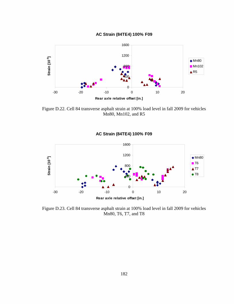
182

AC Strain (84TE4) 100% F09

0

400

800

1200

1600

-30 -20 -10 0 10 20

Rear axle relative offset [in.]

Str

ain

[10-6

]

Mn80Mn102R5

Figure D.22. Cell 84 transverse asphalt strain at 100% load level in fall 2009 for vehicles

Mn80, Mn102, and R5

AC Strain (84TE4) 100% F09

0

400

800

1200

1600

-30 -20 -10 0 10 20

Rear axle relative offset [in.]

Stra

in [1

0-6] Mn80

T6T7T8

Figure D.23. Cell 84 transverse asphalt strain at 100% load level in fall 2009 for vehicles

Mn80, T6, T7, and T8

183

Subgrade Stress (84PG4) 100% F09

0

10

20

30

-30 -20 -10 0 10 20

Rear axle relative offset [in.]

Stre

ss [p

si]

Mn80Mn102R5

Figure D.24. Cell 84 subgrade stress at 100% load level in fall 2009 for vehicles Mn80,

Mn102, and R5

Subgrade Stress (84PG4) 100% F09

0

10

20

30

-30 -20 -10 0 10 20

Rear axle relative offset [in.]

Stra

in [1

0-6] Mn80

T6T7T8

Figure D.25. Cell 84 subgrade stress at 100% load level in fall 2009 for vehicles Mn80,

T6, T7, and T8

184

D.4 Spring 2010

AC Strain (84LE4) 100% S10

0

100

200

300

400

-30 -20 -10 0 10 20 30

Rear axle relative offset [in.]

Stra

in [1

0-6] Mn80

Mn102R6T6

Figure D.26. Cell 84 longitudinal asphalt strain at 100% load level in spring 2010 for

vehicles Mn80, Mn102, R6, and T6

AC Strain (84TE4) 100% S10

0

100

200

300

400

-30 -20 -10 0 10 20 30

Rear axle relative offset [in.]

Stra

in [1

0-6] Mn80

Mn102R6T6

Figure D.27. Cell 84 transverse asphalt strain at 100% load level in spring 2010 for

vehicles Mn80, Mn102, R6, and T6

185

Subgrade Stress (84PG4) 100% S10

0

5

10

15

-30 -20 -10 0 10 20 30

Rear axle relative offset [in.]

Stre

ss [p

si] Mn80

Mn102R6T6

Figure D.28. Cell 84 subgrade stress at 100% load level in spring 2010 for vehicles

Mn80, Mn102, R6, and T6

186

D.5 Fall 2010

AC Strain (84LE4) 100% F10

0

200

400

600

800

-40 -30 -20 -10 0 10 20 30

Rear axle relative offset [in.]

Stra

in [1

0-6]

Mn80Mn102T6

Figure D.29. Cell 84 longitudinal asphalt strain at 100% load level in fall 2010 for

vehicles Mn80, Mn102, and T6

AC Strain (84LE4) 100% F10

0

200

400

600

800

-40 -30 -20 -10 0 10 20 30

Rear axle relative offset [in.]

Stra

in [1

0-6]

Mn80Mn102G1

Figure D.30. Cell 84 longitudinal asphalt strain at 100% load level in fall 2010 for

vehicles Mn80, Mn102, and G1

187

AC Strain (84TE4) 100% F10

0

200

400

600

800

-40 -30 -20 -10 0 10 20 30

Rear axle relative offset [in.]

Stra

in [1

0-6]

Mn80Mn102T6

Figure D.31. Cell 84 transverse asphalt strain at 100% load level in fall 2010 for vehicles

Mn80, Mn102, and T6

AC Strain (84TE4) 100% F10

0

200

400

600

800

-40 -30 -20 -10 0 10 20 30

Rear axle relative offset [in.]

Stra

in [1

0-6]

Mn80Mn102G1

Figure D.32. Cell 84 transverse asphalt strain at 100% load level in fall 2010 for vehicles

Mn80, Mn102, and G1

188

Subgrade Stress (84PG4) 100% F10

0

10

20

30

-40 -30 -20 -10 0 10 20 30

Rear axle relative offset [in.]

Stre

ss [p

si]

Mn80Mn102T6

Figure D.33. Cell 84 subgrade stress at 100% load level in fall 2010 for vehicles Mn80,

Mn102, and T6

Subgrade Stress (84PG4) 100% F10

0

10

20

30

-40 -30 -20 -10 0 10 20 30

Rear axle relative offset [in.]

Stre

ss [p

si]

Mn80Mn102G1

Figure D.34. Cell 84 subgrade stress at 100% load level in fall 2010 for vehicles Mn80,

Mn102, and G1

189

Appendix E Tekscan Measurements

This section includes the measured contact area and average contact stress for vehicles

tested using Tekscan. Contact area and average contact stress were plotted for each of

the vehicle’s axles. The left vertical axes of the following plots correspond to the

measured contact area or average contact stress. The right vertical axes correspond to the

axle weight. Tekscan measurements are shown in Figure E.1 through Figure E.20.

Vehicle S4 Contact Area

0

50

100

150

200

250

300

1 2 3

Axle

Area

[in.

2 ]

0

10,000

20,000

30,000

40,000

50,000

Axle

wei

ght [

lb] 0% area

50% area80% area0% load50% load80% load

Figure E.1. Contact area for vehicle S4 at 0%, 50%, and 80% load levels

190

Vehicle S4 Contact Stress

0

40

80

120

160

1 2 3

Axle

Stre

ss [p

si]

0

10,000

20,000

30,000

40,000

50,000

Axle

wei

ght [

lb] 0% stress

50% stress80% stress0% load50% load80% load

Figure E.2. Average contact stress for vehicle S4 at 0%, 50%, and 80% load levels

Vehicle S5 Contact Area

0

50

100

150

200

250

300

1 2 3

Axle

Are

a [in

.2 ]

0

10,000

20,000

30,000

40,000

50,000

Axle

wei

ght [

lb] 0% area

50% area80% area0% load50% load80% load

Figure E.3. Contact area for vehicle S5 at 0%, 50%, and 80% load levels

191

Vehicle S5 Contact Stress

0

40

80

120

160

1 2 3

Axle

Stre

ss [p

si]

0

10,000

20,000

30,000

40,000

50,000

Axle

wei

ght [

lb] 0% stress

50% stress80% stress0% load50% load80% load

Figure E.4. Average contact stress for vehicle S5 at 0%, 50%, and 80% load levels

Vehicle R4 Contact Area

0

50

100

150

200

250

300

1 2

Axle

Area

[in.

2 ]

0

10,000

20,000

30,000

40,000

50,000

Axle

wei

ght [

lb] 0% area

25% area80% area0% load25% load80% load

Figure E.5. Contact area for vehicle R4 at 0%, 25%, and 80% load levels

192

Vehicle R4 Contact Stress

0

40

80

120

160

1 2

Axle

Stre

ss [p

si]

0

10,000

20,000

30,000

40,000

50,000

Axle

wei

ght [

lb] 0% stress

25% stress80% stress0% load25% load80% load

Figure E.6. Average contact stress for vehicle R4 at 0%, 25%, and 80% load levels

Vehicle R5 Contact Area

0

50

100

150

200

250

300

1 2

Axle

Are

a [in

.2 ]

0

10,000

20,000

30,000

40,000

50,000

Axle

wei

ght [

lb] 0% area

50% area80% area0% load50% load80% load

Figure E.7. Contact area for vehicle R5 at 0%, 50%, and 80% load levels

193

Vehicle R5 Contact Stress

0

40

80

120

160

1 2

Axle

Stre

ss [p

si]

0

10,000

20,000

30,000

40,000

50,000

Axl

e w

eigh

t [lb

] 0% stress50% stress80% stress0% load50% load80% load

Figure E.8. Average contact stress for vehicle R5 at 0%, 50%, and 80% load levels

Vehicle T1 Contact Area

0

50

100

150

200

250

300

1 2 3 4

Axle

Are

a [in

.2 ]

0

10,000

20,000

30,000

40,000

50,000

Axl

e w

eigh

t [lb

] 0% area50% area80% area0% load50% load80% load

Figure E.9. Contact area for vehicle T1 at 0%, 50%, and 80% load levels

194

Vehicle T1 Contact Stress

0

40

80

120

160

1 2 3 4

Axle

Stre

ss [p

si]

0

10,000

20,000

30,000

40,000

50,000

Axl

e w

eigh

t [lb

] 0% stress50% stress80% stress0% load50% load80% load

Figure E.10. Average contact stress for vehicle T1 at 0%, 50%, and 80% load levels

Vehicle T2 Contact Area

0

50

100

150

200

250

300

1 2 3 4

Axle

Are

a [in

.2 ]

0

10,000

20,000

30,000

40,000

50,000

Axl

e w

eigh

t [lb

] 0% area50% area80% area0% load50% load80% load

Figure E.11. Contact area for vehicle T2 at 0%, 50%, and 80% load levels

195

Vehicle T2 Contact Stress

0

40

80

120

160

1 2 3 4

Axle

Stre

ss [p

si]

0

10,000

20,000

30,000

40,000

50,000

Axle

wei

ght [

lb] 0% stress

50% stress80% stress0% load50% load80% load

Figure E.12. Average contact stress for vehicle T2 at 0%, 50%, and 80% load levels

Vehicle T6 Contact Area

0

50

100

150

200

250

300

1 2 3 4

Axle

Are

a [in

.2 ]

0

10,000

20,000

30,000

40,000

50,000

Axl

e w

eigh

t [lb

] 0% area50% area80% area0% load50% load80% load

Figure E.13. Contact area for vehicle T6 at 0%, 50%, and 80% load levels

196

Vehicle T6 Contact Stress

0

40

80

120

160

1 2 3 4

Axle

Stre

ss [p

si]

0

10,000

20,000

30,000

40,000

50,000

Axle

wei

ght [

lb] 0% stress

50% stress80% stress0% load50% load80% load

Figure E.14. Average contact stress for vehicle T6 at 0%, 50%, and 80% load levels

Vehicle T7 Contact Area

0

50

100

150

200

250

300

1 2 3 4 5

Axle

Are

a [in

.2 ]

0

10,000

20,000

30,000

40,000

50,000

Axle

wei

ght [

lb] 0% area

25% area80% area0% load25% load80% load

Figure E.15. Contact area for vehicle T7 at 0%, 25%, and 80% load levels

197

Vehicle T7 Contact Stress

0

40

80

120

160

1 2 3 4 5

Axle

Stre

ss [p

si]

0

10,000

20,000

30,000

40,000

50,000

Axle

wei

ght [

lb] 0% stress

25% stress80% stress0% load25% load80% load

Figure E.16. Average contact stress for vehicle T7 at 0%, 25%, and 80% load levels

Vehicle T8 Contact Area

0

50

100

150

200

250

300

3 4 5 6

Axle

Area

[in.

2 ]

0

10,000

20,000

30,000

40,000

50,000

Axle

wei

ght [

lb]

80% area80% load

Figure E.17. Contact area for vehicle T8 at 80% load level

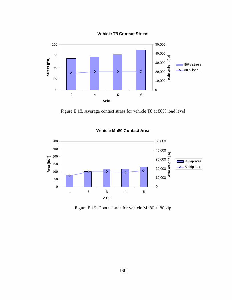
198

Vehicle T8 Contact Stress

0

40

80

120

160

3 4 5 6

Axle

Stre

ss [p

si]

0

10,000

20,000

30,000

40,000

50,000

Axle

wei

ght [

lb]

80% stress80% load

Figure E.18. Average contact stress for vehicle T8 at 80% load level

Vehicle Mn80 Contact Area

0

50

100

150

200

250

300

1 2 3 4 5

Axle

Area

[in.

2 ]

0

10,000

20,000

30,000

40,000

50,000

Axle

wei

ght [

lb]

80 kip area80 kip load

Figure E.19. Contact area for vehicle Mn80 at 80 kip

199

Vehicle Mn80 Contact Stress

0

40

80

120

160

1 2 3 4 5

Axle

Str

ess

[psi

]

0

10,000

20,000

30,000

40,000

50,000

Axl

e w

eigh

t [lb

]

80 kip stress80 kip load

Figure E.20. Average contact stress for vehicle Mn80 at 80 kip