1

Chapter 4

Inductive Loading

4.0 Introduction

This chapter explores the use of inductive loading to increase the radiation resistance

(Rr) and to enable excitation of a grounded tower. Chapter 3 demonstrated the utility

of capacitive top-loading where the increase in Rr was primarily due to beneficial

changes in the current distribution on the vertical. However, top-loading is not the only

means for increasing Rr. We can move the tuning inductor or even only a portion of it,

from the base up into the vertical. We can also move the feedpoint higher in the

vertical. This chapter includes a discussion of multiple-tuning, a technique using

multiple inductors in multiple downleads to manipulate the feedpoint impedance and

distribution of current between parallel wires.

4.1 Loading inductor location

Figure 4.1 - Current distribution on a 50' vertical at 475 kHz.

2

In HF mobile verticals it has long been standard practice to move the loading inductor

from the base up into the vertical to increase Rr[1]. We can do the same for LF/MF

verticals. Figure 4.1 compares the current distribution on a 50' vertical with the tuning

inductor either at the base or near the midpoint. With the inductor near the midpoint

the current below it remains essentially equal to Io. Increasing the current along the

lower part of the vertical increases the Ampere-degree area A' (see section 3.3) which

translates to increased Rr: 0.22Ω → 0.57Ω.

Figure 4.2 - Efficiency as a function of loading inductor location and value.

To keep the antenna resonant as the coil is moved up its impedance (XL) must be

increased, 3411Ω → 6487Ω. Figures 4.2 and 4.3 show efficiency as the coil is moved

higher. In this graph the horizontal axis represents the position of the loading inductor

in percent of total height (H). The vertical axis is the efficiency in decimal form as a

function of inductor placement. Traditionally the entire loading inductance is moved

up. However, there are advantages to moving only a portion of the loading inductance

up into the antenna and retaining the remainder (Lbase) at the base. In figures 4.2 and

3

4.3 the Lbase=0 contour represents the case where all of the inductance is moved up

but there are also contours representing cases where Lbase remains substantial, from

500Ω to 2000Ω. Assuming the same QL for both inductors (QL=400) there can be

some improvement in efficiency with divided loading (≈2%).

Figure 4.3 - Efficiency in dB.

Figure 4.3 converts the decimal efficiencies given in figure 4.2 to dB of signal

improvement. Zero dB corresponds the case where all of the loading inductance is

located at the base. For a given QL, RL will increase as the inductor is moved up.

Despite this increase in RL moving the inductor up generally improves efficiency. The

peak efficiency occurs for heights of 40 to 50% of H. How much does this increase our

signal? For Lbase=0, i.e. we move all the inductance up, we can get about 0.74 dB of

improvement at a height of ≈35%. By making Lbase=1500Ω we can pick up another

0.25 dB for a total improvement of almost 1 dB which is probably worth doing.

4

There is a simple trick for converting XL in ohms to L in μH: XL=2πfL, at 475 kHz

2πfMHz≈3 and at 137 kHz 2πfMHz≈0.86. For example at 475 kHz XL=6487Ω

corresponds to 6487/3≈2,200μH or 2.2mH.

Figure 4.4 - Impedance matching with the base inductor

Even if a modest increase in signal is not compelling there are other reasons for using

two inductors. Even when resonated it will still be necessary to match the feedpoint

impedance to the feedline which can be done very simply by tapping the base

inductance as shown in figure 4.4A.

A base inductor is also a convenient point to retune the antenna when necessary.

Over the course of the seasons as the soil characteristics change, the tuning often

shifts, primarily due to variations in effective loading capacitance as the soil

conductivity changes with moisture content. Small heavily loaded verticals typically

have very narrow bandwidths. In most cases some arrangement for adjusting the

inductance will be needed. This can be readily done by using a variometer (figure

4.4B) (see chapter 6 for details) or a separate small roller inductor in series. One

additional advantage of not putting all the inductance up high is the reduced weight of

the elevated inductor.

5

It is possible to use a long inductor for some or even all of the vertical. This

is occasionally seen in mobile whips. EZNEC Pro v6 can model antennas

constructed with a long helix. Figure 4.5 gives an example of a 50' vertical

with a helix (coil) 24' long, 2' in diameter, with150 turns of #12 copper wire.

The bottom of the coil is at 2' and the top of the coil at 26'. EZNEC gives an

efficiency of ≈4.1% which is somewhat better than a single concentrated

load at 0.35H (figure 4.2, QL=400).

Figure 4.5 - A 475 kHz vertical with distributed loading inductor.→

4.2 Inductor location with top-loading

Due to windage considerations mobile verticals seldom have much

capacitive top-loading but fixed station antennas have (or should have!) as

much top-loading as practical.

Figure 4.6 - Efficiency as a function of loading coil position.

6

Figure 4.7 - Efficiency versus loading coil position with heavy top-loading.

Moving the inductor higher into a heavily top-loaded vertical has less effect on the

current distribution. As a result efficiency improvements are much smaller. Figure 4.6

gives an example of a T antenna with H= 50' and a single 100' top-wire. As the

inductor is moved up there is some improvement in the signal but not a lot, only 0.4 dB

even when two inductors are used.

As shown in figure 4.7, when we have a much larger top-hat (three wires 100' long by

20' wide) the improvement from elevating the inductor is even smaller, <0.15 dB This

small an improvement is not worth the hassle of mounting an inductor high in the

antenna! The reason for the very small improvement can be seen in figure 4.8 which

shows the current distribution for various loading inductor heights. Even without

moving the inductor up, It/Io is almost 0.85 (It=current at the top of the vertical section).

Moving the inductor up increases A' but not by very much.

7

Figure 4.8 - Current distributions on a top-loaded vertical for various loading inductor

heights at 475 kHz.

In heavily top-loaded verticals there appears to be little improvement in efficiency from

elevating the loading inductor. On the other hand if the top-loading is less, It/Io ratio

<0.4-0.5, and more top-loading is not practical then moving the coil up may help. This

has to be evaluated on a case-by-case basis using modeling.

4.3 Grounded Tower Verticals

A grounded tower with attached HF antennas and associated cabling is sometimes

available. For an LF-MF antenna the tower may be simply a support but it can also be

a radiator. One way we might do this is shown in figure 4.9 where the loading inductor

and the feedpoint have been moved to the top of the tower. The top-loading wires are

insulated from the tower and connected to one end of the loading inductor. The other

end of the inductor is connected to the top of the tower. A coaxial feedline runs up the

tower with the shield connected to the top of the tower. The coax center conductor is

8

connected to a tap on the loading inductor to provide a match. Although not shown, it

is possible to have a mast with HF Yagis extending above the top of the tower which

will add some additional capacitive loading. The downside of this scheme is that all the

adjustments must be made at the top of the tower.

Figure 4.9 - Grounded tower, feedpoint and loading inductor at the top.

A common alternative for exciting a grounded tower often used on 80m and 160m is

the shunt-fed tower shown in figure 4.10. Unfortunately this scheme works only if

H>0.7 λ/4 at the operating frequency. At 475 kHz that would mean H>350', much taller

than most amateur towers. The causes and cures for problems associated with this

configuration are worth discussing in some detail because similar problems can arise

whenever multiple downleads are used, which is quite common in LF-MF antennas.

9

Figure 4.10 - Shunt fed tower.

Figure 4.11 - Monopole antenna. From

Raines[6]

The arrangement illustrated in figure 4.10 is usually considered to be an impedance

matching scheme but the tower and the shunt wire is actually a member of a family of

antennas called "folded monopoles", as shown in figure 4.11. One of the important

properties of folded monopoles is that the feedpoint impedance can be a multiple of

that for a single element vertical of the same height. For example, if two elements are

used and both elements have the same diameter, the Zi will be 4X that for a single

element. Even more elements can be added to further increase Ri. It is also possible

to use elements of different diameters which can lead to arbitrary Ri ratios. All of this

however, applies only when the height is close to λ/4. When we shorten the antenna

to heights practical on 475 or 137 kHz the antenna behavior is quite different.

10

Figure 4.12 - Ri versus height for normal and folded monopoles.

Figure 4.12 compares the values of feedpoint Ri between a normal monopole (dashed

line) and a folded monopole (solid line) at 475 kHz for a wide range of heights. Ri for

the normal monopole has been multiplied by 4X for this comparison. A similar graph

for Xi is given in figure 4.13. In both graphs we can see that for heights down to ≈400'

Zi ≈ 4X as predicted but as we go to shorter heights there is a rapid divergence

between the behavior of the two antennas. Our interest is primarily H<100' where the

folded monopole impedance is very small compared to the normal monopole.

What's going on and can we fix it?

11

figure 4.13 - Xi versus height for normal and folded monopoles.

A folded monopole can be viewed as a superposition of a vertical and a transmission

line shorted at the far end as shown in 4.14[5, 6, 7, 8]. There are two currents, a radiating

"antenna current" =2X(Ia/2) and a circulating "transmission line current" =IT. A lumped

element equivalent circuit is shown where Ra+jXa represents the vertical and +jXT

represents the inductance appearing across the feedpoint due to the transmission line.

The value for jXT can be found from:

jXT=jZo Tan(H)

Where Zo is the characteristic impedance of the transmission line which depends on

element spacing and diameters. H is the length in degrees or radians.

For the "monopole" Xc rises quickly as H is reduced (chapter 2) but the "transmission

line" XT falls rapidly as H is reduced. The result is shown in figure 4.13, at H≈310',

12

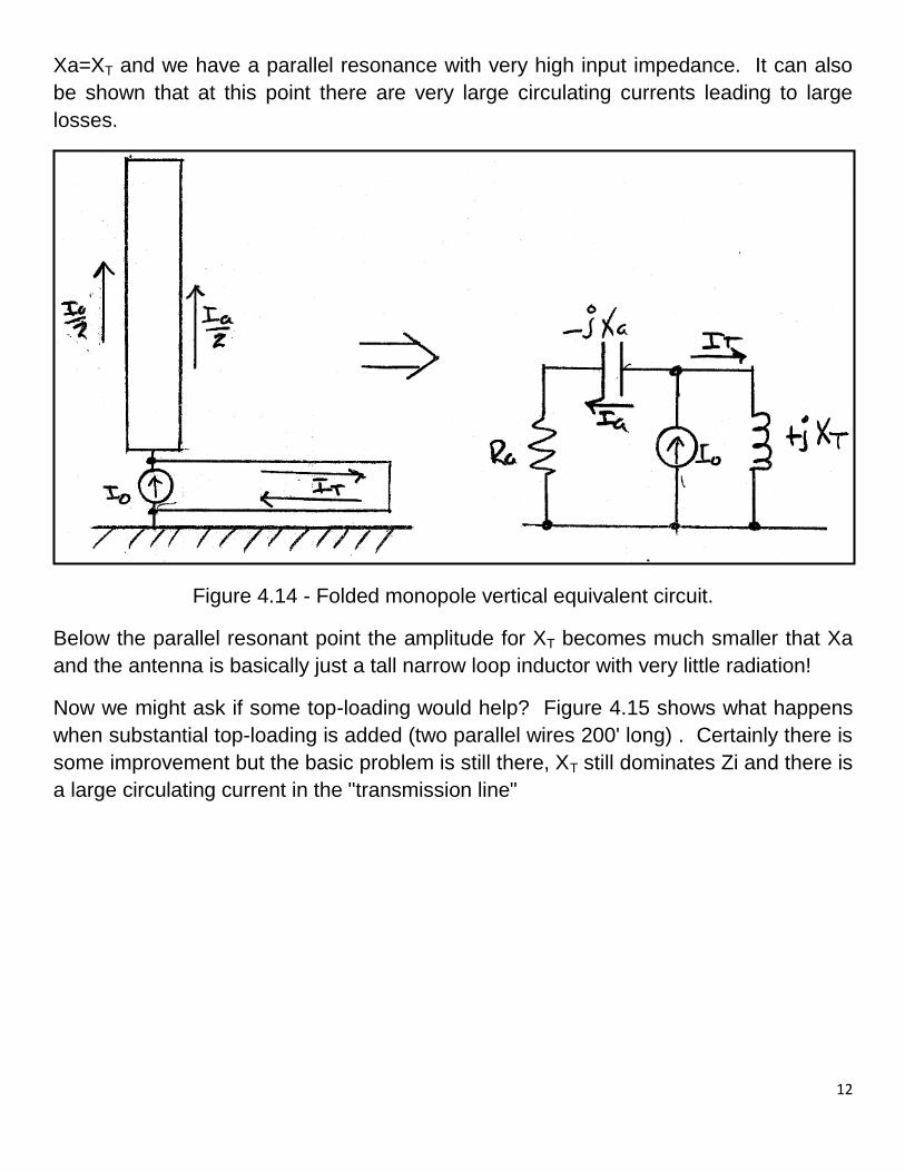
Xa=XT and we have a parallel resonance with very high input impedance. It can also

be shown that at this point there are very large circulating currents leading to large

losses.

Figure 4.14 - Folded monopole vertical equivalent circuit.

Below the parallel resonant point the amplitude for XT becomes much smaller that Xa

and the antenna is basically just a tall narrow loop inductor with very little radiation!

Now we might ask if some top-loading would help? Figure 4.15 shows what happens

when substantial top-loading is added (two parallel wires 200' long) . Certainly there is

some improvement but the basic problem is still there, XT still dominates Zi and there is

a large circulating current in the "transmission line"

13

Figure 4.15 - Ri versus height for normal and top-loaded folded monopoles.

Figure 4.16 shows we might eliminate the effect of XT by adding series inductance

(XL). There are a couple of points at which we might add inductance: at the grounded

end of element 1 or at the top of the antenna or both. Since our concern here is with a

grounded tower we will place an inductor at the top of the antenna. Other possibilities

are discussed in the section on multiple tuning. If XL>> XT then the transmission line

impedance is in effect constant and has a value of our choosing. Normally we would

choose XL to resonate the antenna which means it's value will be large compared to XT

for typical amateur antenna heights. Figure 4.17 shows an application of this idea with

part of the loading inductor at the top and the rest at ground level to make adjustment

and matching convenient. Even though we've overcome a problem with short folded

monopoles, we still have a very short vertical so in addition to the inductive loading we

still need capacitive top-loading as shown to minimize the inductance. The top-hat

wires are insulated from the tower as they were in figure 4.9.

14

figure 4.16 - Alternate impedance placement. From Raines[tbd] & Harrison & King[5].

Figure 4.17 - Grounded tower feed scheme using two inductors.

15

4.4 Multiple Tuning

As suggested in figure 4.18, we can have multiple vertical elements, 1,2,...,m, n,... with

inductors in series with each downlead/vertical.

Figure 4.18 - Adding tuning inductors to a short folded monopole. From Raines[6]

Commercial LF antennas have long used multiple inductors to advantage. An example

taken from Laport[2] is shown in figure 4.19.

Figure 4.19 - Example of multiple tuning.

The following is a quotation from Laport:

"The most extreme conditions of low radiation resistance and high

reactance are encountered at the lowest frequencies, and some extreme

16

measures are necessary to obtain acceptable radiation efficiencies. .......

The most successful method of improving the radiation efficiency is that of

multiple tuning. The antenna consists of a large elevated capacitance area

with two or more down leads that are tuned individually as indicated in

the figure. The total antenna current is thus divided equally among the

down leads, each of which has its own ground system. The down lead

currents are in phase, and because of their electrically small separation

there is no observable effect on the radiation pattern, which is always

nearly circular. Power is fed into the system through one of the down

leads.

When arranged for multiple tuning, an antenna behaves as a number of

smaller antennas in parallel, voltage being fed through the flat-top system.

Thus, a system with triple tuning is essentially three antennas in parallel,

one of which is fed directly by coupling to the transmitter and the other

two at high potential (voltage feed) through their common flat-top. From a

radiation standpoint, the same effect would be realized if the different

portions of the antenna were not physically connected through their

common flat-top but instead were separately fed from a common

transmitter and feeder system in the manner of a directive antenna.

Practically it is simpler to take advantage of the fact that almost all

antennas for the lowest radio frequencies must of necessity employ flat-tops

for capacitive loading and merely to add the extra down leads for multiple

tuning. In that way, there is only one feed point, and the problems of

power division, phasing, and impedance matching are automatically

minimized. .....

If N represents the number of multiple tuning down leads carrying equal

currents, the new radiation resistance Rrr is related to that for single

tuning by the equation

Rrr=RrN2. ...."

In a short LF-MF antenna this scheme can provide feedpoint impedances which are

much easier to deal with. Laport goes on to suggest that, for equal QL in all inductors,

the total inductor loss will be reduced with multiple tuning but this does not appear to

be correct. Modeling shows that the losses are essentially the same. However,

ground system losses with multiple grounds may be less.

17

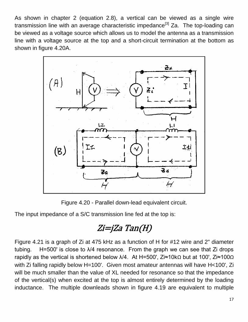
As shown in chapter 2 (equation 2.8), a vertical can be viewed as a single wire

transmission line with an average characteristic impedance[3] Za. The top-loading can

be viewed as a voltage source which allows us to model the antenna as a transmission

line with a voltage source at the top and a short-circuit termination at the bottom as

shown in figure 4.20A.

Figure 4.20 - Parallel down-lead equivalent circuit.

The input impedance of a S/C transmission line fed at the top is:

Zi=jZa Tan(H)

Figure 4.21 is a graph of Zi at 475 kHz as a function of H for #12 wire and 2" diameter

tubing. H=500' is close to λ/4 resonance. From the graph we can see that Zi drops

rapidly as the vertical is shortened below λ/4. At H=500', Zi≈10kΩ but at 100', Zi≈100Ω

with Zi falling rapidly below H=100'. Given most amateur antennas will have H<100', Zi

will be much smaller than the value of XL needed for resonance so that the impedance

of the vertical(s) when excited at the top is almost entirely determined by the loading

inductance. The multiple downleads shown in figure 4.19 are equivalent to multiple

18

transmission lines in parallel as shown in figure 4.20B. To control the current

distribution between the multiple downleads we insert inductors. The currents may all

be the same as or different. Non-equal current distributions can be used to modify the

feedpoint impedance, i.e. if you insert more inductance in the driven downlead, the

current that downlead will be reduced and the feedpoint impedance increased. You

will have to readjust the other inductances to re-resonate the antenna however!

Figure 4.21 - Zi at 475 kHz versus height.

One other important point, Terman[4, page 841] has a comment on minimum top-hat

capacitance which applies to multiple tuning:

"...the flat-top capacitance should be considerably greater than the

capacity of the vertical downlead....."

There has to be enough capacitance so that the impedance of the "voltage source" (i.e.

the top-loading) is low compared to Zi.

19

4.5 Multiple tuning examples

As a reference point we can start with the T antenna shown in figure 4.22.

Figure 4.22 - T-antenna example.

Figure 4.23 - Antenna with two downleads and a loading inductor at the base of each

downlead.

20

The antenna and the radials are #12 copper wire. H=50' and each top-wire is 50' long.

There are sixty four 45' radials buried 6" in average soil (0.005/13). For resonance at

475 kHz, XL=1239Ω (≈410μH). Including copper (Rc), RL and soil losses (Rg), the

feedpoint resistance Ri is ≈6.21Ω and the radiation efficiency is ≈10.0% or -10dB.

Suppose we use the same top-wire (100') but introduce multiple tuning with two

downleads, one at each end as shown in figure 4.23.

For each downlead H=50' and the top-wire is 2x50'=100'. The same total amount of

wire is used in the new ground system, i.e. each downlead has thirty two 45' radials.

For resonance at 475 kHz, XL1=XL2= 1857Ω (≈620 uH). Ri≈16.3Ω and the efficiency

is about 11.9% or -9.24 dB which represents a signal improvement of +0.76 dB. As

predicted going from one to two downleads the current in each downlead is Io/2 and Ri

is increased by a factor of four. There is some improvement in efficiency, ≈2%. It

should also be noted that the antenna in figure 4.23 forms a half-loop. In regions

subject to ice storms it is possible to inject a line frequency current at the base of the

driven element and add a ground wire between the bases to complete an AC heater

circuit.

Figure 4.24 - Increased top-loading.

21

We could have used more top-loading (figure 4.24) to increase efficiency. This

increases the efficiency to 15.1% or +1.8 dB which is almost 1 dB better than the

multiple tuning example in figure 4.23. Of course we could also combine multiple

tuning with the increased top-loading as shown in figure 4.25. The efficiency is now

18.6% or -7.3 dB. In this example multiple tuning increases the signal by another dB.

Multiple tuning can increase efficiency but usually only modestly.

Figure 4.25 - Multiple tuning applied to figure 4.24.

22

4.6 Loop antennas

Ground systems are a nuisance and sometimes impractical. We might consider using

a transmitting loop like that shown in figure 4.26.

Figure 4.26 - Loop antenna.

In this example the horizontal wires are 100' long and the vertical wires 50', all #12

copper wire. The bottom wire is 8' above average ground (0.005/13) and f=475 kHz.

The antenna is resonated with a capacitive load at the center of the upper wire (3)

where Xc=537Ω. As is typical for small loops the current amplitude around the loop

varies only +/- 5% with very little phase difference and for the values given, the

radiation efficiency will be ≈1.8%. John Andrews, W1TAG, WE2XGR/3, has used a

similar loop made with RG8 coax (diameter≈0.3"). This increases the efficiency to

≈3.1%. Not great but if 100W of input power is available then the maximum EIRP can

be reached. Even if we used super-conducting wire the efficiency would still be limited

to ≈4.2% due to near-field ground losses, a factor often overlooked in transmitting

loops. Poorer soil would mean even lower efficiency. These efficiencies are not very

23

encouraging but then transmitting loop antennas are not known for their efficiency!

This antenna has a directive pattern with a mix of vertical and horizontal radiation

shown in figure 4.27.

Figure 4.27 - V and H radiation pattern at 23° elevation.

This discussion raises the question "can we use inductors to improve transmitting loop

efficiency?" Suppose we take the antenna in figure 4.23 and elevate it 8' above

ground and replace the ground system with a single wire as shown in figure 4.28. The

loads are equal, XL1=XL2= 4443Ω for resonance at 475 kHz. The antenna has the

same dimensions and construction as the loop in figure 4.26. However, the current

pattern is very different! The currents in horizontal wires are out of phase, with a null at

the center of the horizontal wires. The currents in the downleads are now in-phase.

24

Figure 4.28 - Loop currents with multiple tuning inductors.

Figure 4.29 - Directional pattern with multiple tuning.

25

This results in a very different radiation pattern as shown in figure 4.29. The radiation

is almost all vertically polarized and uniform in all directions. The efficiency including

conductor and soil losses has been increased from 1.8% to 8.9%, almost 5X!

It is important to recognize that by adding two inductors to a

small transmitting loop (0.14λ circumference) we have

transformed the current distribution making it a very

different antenna!

Figure 4.30 - Adding top and bottom capacitive loading.

Returning to figure 4.28, 8.9% is a significant improvement over the conventional loop

but still no great shakes. In the case of the simple loop, conductor loss is important but

in the multi-tuned loop the losses are dominated by loading inductor RL. We know

how to reduce RL: add capacitive loading! Figure 4.30 gives an example. The

efficiency of this configuration is ≈12.8%, far higher than the simple loop. It's still not

as good as antennas with ground systems (figures 4.24 and 4.25) but then there is no

ground system. A fair trade perhaps?

26

4.7 Effect of feedpoint location

Although it's very convenient to feed a vertical directly at the base we don't have to. In

short LF/MF verticals we can modify the current distribution by placing the feedpoint

some distance up the vertical.

In a full size λ/4 vertical we can ground the base and place the source at any point

along the conductor. You could for example insert an insulator at some elevated point

with the coaxial feedline inside the vertical up to the insulator with the shield connected

to the lower section of the antenna at that point and the center conductor connected to

the upper section. The base of the vertical is grounded. When you do this the antenna

is still resonant but, depending on the placement of the insulator, the feedpoint

impedance can now be 50Ω or whatever you wish. This is a common trick at HF to

improve the SWR without a matching network. However:

When you do this in a λ/4 vertical there is no detectable change in the current

distribution along the vertical, i.e. A' is not changed.

Figure 4.31 - Effect on current distribution of different feedpoint locations.

27

When you play this same game with a short vertical, say H=50' at 475 kHz, the current

distribution and A' changes greatly! As shown in figure 4.31, the current below the

feedpoint is nearly constant. Elevating the feedpoint increases A' which implies an

increase in Rr. While the increase in Rr from moving the tuning inductor up into the

antenna has long been known I've never see the effect of moving the source

discussed.

This effect is interesting but it does not appear to be particularly useful for LF/MF

transmitting antennas because there will be a large tuning reactance which can be

moved to increase Rr. If we try to leave the tuning inductor at the base and only

elevate the feedpoint then we have the problem of decoupling the feedline at the base.

If the base inductor is wound with coaxial line then the base inductor can provide the

decoupling but that complicates the tuning inductor. However, this scheme does allow

us to obtain higher Rr without having to elevate the loading inductor.

While not particularly useful for transmitting verticals an elevated feedpoint can be very

useful when short verticals (e-probes) are used as elements in a receiving array.

These verticals are normally not resonated with loading inductors but simply connected

to the inputs of high impedance amplifiers. Moving the feedpoint up into the e-probe

increases A' which increases the effective height (h) which increases the terminal

voltage for a given E-field intensity. It should also be kept in mind that adding top-

loading to an e-probe will also increase the effective height.

Summary

This chapter has shown several variations for the placement and number of loading

inductors. Once the antenna height and top-loading have been maximized the

following points were made:

...loading inductor arrangements can significantly improve the

efficiency...

...and make it possible to excite a grounded tower to act as

radiating part of the antenna...

...for a receiving e-probe vertical, moving the feedpoint up into

the vertical can increase the received signal....

28

References

[1] ARRL Antenna Book, any edition, chapter on mobile antennas.

[2] Laport, Edmund, Radio Antenna Engineering, McGraw-Hill, 1952. You can find this

one free on-line by Googling Edmund Laport.

[3] Schelkunoff and Friis, Antennas, Theory and Practice, page 426

[4] Terman, Frederick E., Radio Engineers Handbook, McGraw-Hill Book Company,

1943

[5] Harrison and King, Folded Dipoles and Loops, IRE AP transactions, March 1961,

pp. 171-187

[6] Raines, Jeremy, Folded Unipole Antennas, McGraw-Hill, 2007

[7] Guertler, Rudolf, Impedance Transformation in Folded Dipoles, IRE Proceedings,

September 1950, pp. 1042-1047

[8] Leonhard, Mattuck and Pote', Folded Unipole Antennas, IRE AP Transactions, July

1955, pp. 111-116