Embed Size (px)
Citation preview
Effect of the Gribov horizon on the Polyakov loop
and vice versa
F. E. Canforaa∗, D. Dudalb,c†, I. F. Justoc,d‡,P. Paisa,e§, L. Rosaf,g¶, D. Vercauterenh‖
a Centro de Estudios Científicos (CECS), Casilla 1469, Valdivia, Chileb KU Leuven Campus Kortrijk - KULAK, Department of Physics,
Etienne Sabbelaan 53, 8500 Kortrijk, Belgiumc Ghent University, Department of Physics and Astronomy
Krijgslaan 281-S9, 9000 Gent, Belgiumd Departamento de Física Teórica, Instituto de Física, UERJ - Universidade do Estado do Rio de Janeiro,
Rua São Francisco Xavier 524, 20550-013 Maracanã, Rio de Janeiro, Brazile Physique Théorique et Mathématique, Université Libre de Bruxelles
and International Solvay Institutes, Campus Plaine C.P. 231, B-1050 Bruxelles, Belgiumf Dipartimento di Fisica, Universitá di Napoli Federico II, Complesso Universitario di Monte S. Angelo,
Via Cintia Edificio 6, 80126 Napoli, Italiag INFN, Sezione di Napoli, Complesso Universitario di Monte S. Angelo,
Via Cintia Edificio 6, 80126 Napoli, Italiah Duy Tân University, Institute of Research and Development,
P809, K7/25 Quang Trung, Hải Châu, Đà Nẵng, Vietnam
Abstract
We consider finite temperature SU(2) gauge theory in the continuum formulation, which necessi-tates the choice of a gauge fixing. Choosing the Landau gauge, the existing gauge copies are taken intoaccount by means of the Gribov–Zwanziger (GZ) quantization scheme, which entails the introduc-tion of a dynamical mass scale (Gribov mass) directly influencing the Green functions of the theory.Here, we determine simultaneously the Polyakov loop (vacuum expectation value) and Gribov massin terms of temperature, by minimizing the vacuum energy w.r.t. the Polyakov loop parameter andsolving the Gribov gap equation. Inspired by the Casimir energy-style of computation, we illustratethe usage of Zeta function regularization in finite temperature calculations. Our main result is thatthe Gribov mass directly feels the deconfinement transition, visible from a cusp occurring at the sametemperature where the Polyakov loop becomes nonzero. In this exploratory work we mainly restrictourselves to the original Gribov–Zwanziger quantization procedure in order to illustrate the approachand the potential direct link between the vacuum structure of the theory (dynamical mass scales) and(de)confinement. We also present a first look at the critical temperature obtained from the RefinedGribov–Zwanziger approach. Finally, a particular problem for the pressure at low temperatures isreported.
∗[email protected]†[email protected]‡[email protected]§[email protected]¶[email protected]‖[email protected]
1
arX
iv:1
505.
0228
7v2
[he
p-th
] 2
9 Ju
n 20
15

1 Introduction
Within SU(N) Yang-Mills gauge theories, it is well accepted that the asymptotic particle spectrum doesnot contain the elementary excitations of quarks and gluons. These color charged objects are confinedinto color neutral bound states: this is the so-called color confinement phenomenon. It is widely believedthat confinement arises due to non-perturbative infrared effects. Many criteria for confinement have beenproposed (see the nice pedagogical introduction [1]). A very natural observation is that gluons (due tothe fact that they are not observed experimentally) should not belong to the physical spectrum in aconfining theory. On the other hand, the perturbative gluon propagator satisfies the criterion to belongto the physical spectrum (namely, it has a Kallén-Lehmann spectral representation with positive spectraldensity). Hence, non-perturbative effects must dress the perturbative propagator in such a way thatthe positivity conditions are violated, such that it does not belong to the physical spectrum anymore.A well-known criterion is related to the fact that the Polyakov loop [2] is an order parameter for theconfinement/deconfinement phase transition via its connection to the free energy of a (very heavy) quark.The importance to clarify the interplay between these two different points of view (nonperturbative Greenfunction’s behaviour vs. Polyakov loop) can be understood by observing that while there are, in principle,infinitely many different ways to write down a gluon propagator which violates the positivity conditions,it is very likely that only few of these ways turns out to be compatible with the Polyakov criterion.
One of the most fascinating non-perturbative infrared effects is related to the appearance of Gribovcopies [3] which represent an intrinsic overcounting of the gauge-field configurations which the perturba-tive gauge-fixing procedure is unable to take care of. Soon after Gribov’s seminal paper, Singer showedthat any true gauge condition, as the Landau gauge1, presents this obstruction [4] (see also [5]). Thepresence of Gribov copies close to the identity induces the existence of non-trivial zero modes of theFaddeev-Popov operator, which make the path integral ill defined. Even when perturbation theoryaround the vacuum is not affected by Gribov copies close to the identity (in particular, when YM-theoryis defined over a flat space-time2 with trivial topology [10]), Gribov copies have to be taken into ac-count when considering more general cases (such as with toroidal boundary conditions on flat space-time[11, 12]). Thus, in the following only the standard boundary conditions will be considered.
The most effective method to eliminate Gribov copies, at leading order proposed by Gribov himself,and refined later on by Zwanziger [3, 13, 14, 15] corresponds to restricting the path integral to theso-called Gribov region, which is the region in the functional space of gauge potentials over which theFaddeev-Popov operator is positive definite. The Faddeev–Popov operator is Hermitian in the Landaugauge, so it makes sense to discuss its sign. In [16, 17] Dell’Antonio and Zwanziger showed that all theorbits of the theory intersect the Gribov region, indicating that no physical information is lost whenimplementing this restriction. Even though this region still contains copies which are not close to theidentity [18], this restriction has remarkable effects. In fact, due to the presence of a dynamical (Gribov)mass scale, the gluon propagator is suppressed while the ghost propagator is enhanced in the infrared.More general, an approach in which the gluon propagator is “dressed” by non-perturbative correctionswhich push the gluon out of the physical spectrum leads to propagators and glueball masses in agreementwith the lattice data [19, 20]. With the same approach, one can also solve the old problem of theCasimir energy in the MIT-bag model [21]. Moreover, the extension of the Gribov gap equation atfinite temperature provides one with a good qualitative understanding, already within the semiclassicalapproximation, of the deconfinement temperature as well as of a possible intermediate phase in whichfeatures of the confining phase coexist with features of the fully deconfined phase in agreement withdifferent approaches (see [22] and references therein). Furthermore, within this framework the presenceof the Higgs field [23, 24] as well of a Chern-Simons term in 2+1 dimensions [25] can be accounted for aswell.
For all these reasons, it makes sense to compute the vacuum expectation value of the Polyakov loopwhen we eliminate the Gribov copies using the Gribov–Zwanziger (GZ) approach. Related computationsare available using different techniques to cope with nonperturbative propagators at finite temperature,see e.g. [26, 27, 28, 29, 30, 31, 32, 33, 34, 35, 36]. In the present paper, we will perform for the first time (to
1We shall work exclusively with the Landau gauge here.2In the curved case, the pattern of appearance of Gribov copies can be considerably more complicated: see in particular
[6, 7, 8, 9]. Therefore, only the flat case will be considered here.
2
the best of the authors’ knowledge) this computation, using two different techniques, to the leading one-loop approximation. In [37, 38, 39], it was already pointed out that the Gribov–Zwanziger quantizationoffers an interesting way to illuminate some of the typical infrared problems for finite temperature gaugetheories.
In Section 2, we provide a brief technical overview of the Gribov–Zwanziger quantization process andeventual effective action. In the following Section 3, the Polyakov loop is introduced into the GZ theoryvia the background field method, building on work of other people [27, 28, 32]. Next, Section 4 handlesthe technical computation of the leading order finite temperature effective action, while in Section 5 wediscuss the gap equations, leading to our estimates for both Polyakov loop and Gribov mass. The keyfinding is a deconfinement phase transition at the same temperature at which the Gribov mass develops acuspy behaviour. We subsequently also discuss the pressure and energy anomaly. Due to a problem withthe pressure in the GZ formalism (regions of negativity), we take a preliminary look at the situation uponinvoking the more recently developed Refined Gribov–Zwanziger approach. We summarize in Section 7.
2 A brief summary of the Gribov–Zwanziger action in Yang–Mills theories
Let us start by giving a short overview of the Gribov–Zwanziger framework [3, 13, 14, 15]. As alreadymentioned in the Introduction, the Gribov–Zwanziger action arises from the restriction of the domain ofintegration in the Euclidean functional integral to the Gribov region Ω, which is defined as the set ofall gauge field configurations fulfilling the Landau gauge, ∂µAaµ = 0, and for which the Faddeev–PopovoperatorMab = −∂µ(∂µδ
ab − gfabcAcµ) is strictly positive, namely
Ω = Aaµ ; ∂µAaµ = 0 ; Mab = −∂µ(∂µδ
ab − gfabcAcµ) > 0 .
The boundary ∂Ω of the region Ω is the (first) Gribov horizon.
One starts with the Faddeev–Popov action in the Landau gauge
SFP = SYM + Sgf , (1)
where SYM and Sgf denote, respectively, the Yang–Mills and the gauge-fixing terms, namely
SYM =1
4
∫d4x F aµνF
aµν , (2)
andSgf =
∫d4x
(ba∂µA
aµ + ca∂µD
abµ c
b), (3)
where (ca, ca) stand for the Faddeev–Popov ghosts, ba is the Lagrange multiplier implementing the Landaugauge, Dab
µ = (δab∂µ − gfabcAcµ) is the covariant derivative in the adjoint representation of SU(N), andF aµν denotes the field strength:
F aµν = ∂µAaν − ∂νAaµ + gfabcAbµA
cν . (4)
Following [3, 13, 14, 15], the restriction of the domain of integration in the path integral is achieved byadding to the Faddeev–Popov action SFP an additional term H(A), called the horizon term, given by thefollowing non-local expression
H(A, γ) = g2
∫d4x d4y fabcAbµ(x)
[M−1(γ)
]ad(x, y)fdecAeµ(y) , (5)
where M−1 stands for the inverse of the Faddeev–Popov operator. The partition function can then bewritten as [3, 13, 14, 15]:
ZGZ =
∫Ω
DA Dc Dc Db e−SFP =
∫DA Dc Dc Db e−(SFP+γ4H(A,γ)−V γ44(N2−1)) , (6)
3

where V is the Euclidean space-time volume. The parameter γ has the dimension of a mass and is knownas the Gribov parameter. It is not a free parameter of the theory. It is a dynamical quantity, beingdetermined in a self-consistent way through a gap equation called the horizon condition [3, 13, 14, 15],given by
〈H(A, γ)〉GZ = 4V(N2 − 1
), (7)
where the notation 〈H(A, γ)〉GZ means that the vacuum expectation value of the horizon functionH(A, γ)has to be evaluated with the measure defined in Eq.(6). An equivalent all-order proof of eq.(7) can begiven within the original Gribov no-pole condition framework [3], by looking at the exact ghost propagatorin an external gauge field [40].
Although the horizon term H(A, γ), eq.(5), is non-local, it can be cast in local form by means of theintroduction of a set of auxiliary fields (ωabµ , ω
abµ , ϕ
abµ , ϕ
abµ ), where (ϕabµ , ϕ
abµ ) are a pair of Bosonic fields,
while (ωabµ , ωabµ ) are anti-commuting. It is not difficult to show that the partition function ZGZ in eq.(6)
can be rewritten as [13, 14, 15]
ZGZ =
∫DΦ e−SGZ[Φ] , (8)
where Φ accounts for the quantizing fields, A, c, c, b, ω, ω, ϕ, and ϕ, while SGZ[Φ] is the Yang–Millsaction plus gauge fixing and Gribov–Zwanziger terms, in its localized version,
SGZ = SYM + Sgf + S0 + Sγ , (9)
withS0 =
∫d4x
(ϕacµ (−∂νDab
ν )ϕbcµ − ωacµ (−∂νDabν )ωbcµ + gfamb(∂ν ω
acµ )(Dmp
ν cp)ϕbcµ), (10)
andSγ = γ2
∫d4x
(gfabcAaµ(ϕbcµ + ϕbcµ )
)− 4γ4V (N2 − 1) . (11)
It can be seen from (6) that the horizon condition (7) takes the simpler form
∂Ev∂γ2
= 0 , (12)
which is called the gap equation. The quantity Ev(γ) is the vacuum energy defined by
e−V Ev = ZGZ . (13)
The local action SGZ in eq.(9) is known as the Gribov–Zwanziger action. Remarkably, it has beenshown to be renormalizable to all orders [13, 14, 15, 41, 42, 43, 44, 45]. This important property ofthe Gribov–Zwanziger action is a consequence of an extenstive set of Ward identities constraining thequantum corrections in general and possible divergences in particular. In fact, introducing the nilpotentBRST transformations
sAaµ = −Dabµ c
b ,
sca =1
2gfabccbcc ,
sca = ba , sba = 0 ,
sωabµ = ϕabµ , sϕabµ = 0 ,
sϕabµ = ωabµ , sωabµ = 0 , (14)
it can immediately be checked that the Gribov–Zwanziger action exhibits a soft breaking of the BRSTsymmetry, as summarized by the equation
sSGZ = γ2∆ , (15)
where∆ =
∫d4x
(−gfabc(Dam
µ cm)(ϕbcµ + ϕbcµ ) + gfabcAaµωbcµ
). (16)
4
Notice that the breaking term ∆ is of dimension two in the fields. As such, it is a soft breaking and theultraviolet divergences can be controlled at the quantum level. The properties of the soft breaking of theBRST symmetry of the Gribov–Zwanziger theory and its relation with confinement have been object ofintensive investigation in recent years, see [46, 47, 48, 49, 50, 51, 52, 53, 54, 55]. Here, it suffices to mentionthat the broken identity (15) is connected with the restriction to the Gribov region Ω. However, a setof BRST invariant composite operators whose correlation functions exhibit the Kallén-Lehmann spectralrepresentation with positive spectral densities can be consistently introduced [56]. These correlationfunctions can be employed to obtain mass estimates on the spectrum of the glueballs [19, 20].
Let us conclude this brief review of the Gribov–Zwanziger action by noticing that the terms Sgf andS0 in expression (9) can be rewritten in the form of a pure BRST variation, i.e.
Sgf + S0 = s
∫d4x
(ca∂µA
aµ + ωacµ (−∂νDab
ν )ϕbcµ), (17)
so thatSGZ = SYM + s
∫d4x
(ca∂µA
aµ + ωacµ (−∂νDab
ν )ϕbcµ)
+ Sγ , (18)
from which eq.(15) becomes apparent.
3 The Polyakov loop and the background field formalism
In this section we shall investigate the confinement/deconfinement phase transition of the SU(2) gaugefield theory in the presence of two static sources of (heavy) quarks. The standard way to achieve thisgoal is by probing the Polyakov loop order parameter,
P =1
Ntr⟨Peig
∫ β0dt A0(t,x)
⟩, (19)
with P denoting path ordering, needed in the non-Abelian case to ensure the gauge invariance of P.This path ordering is not relevant at one-loop order, which will considerably simplify the computationsof the current work. In analytical studies of the phase transition involving the Polyakov loop, one usuallyimposes the so-called “Polyakov gauge” on the gauge field, in which case the time-component A0 becomesdiagonal and independent of (imaginary) time. This means that the gauge field belongs to the Cartansubalgebra. More details on Polyakov gauge can be found in [28, 57, 58]. Besides the trivial simplificationof the Polyakov loop, when imposing the Polyakov gauge it turns out that the quantity 〈A0〉 becomes agood alternative choice for the order parameter instead of P. This extra benefit can be proven by meansof Jensen’s inequality for convex functions and is carefully explained in [28], see also [27, 29, 30, 31, 32].For example, for the SU(2) case we have the following: if 1
2gβ 〈A0〉 = π2 then we are in the “unbroken
symmetry phase” (confined or disordered phase), equivalent to 〈P〉 = 0; otherwise, if 12gβ 〈A0〉 < π
2 ,we are in the “broken symmetry phase” (deconfined or ordered phase), equivalent to 〈P〉 6= 0. SinceP ∝ e−FT with T the temperature and F the free energy of a heavy quark, it is clear that in theconfinement phase, an infinite amount of energy would be required to actually get a free quark. Thebroken/restored symmetry referred to is the ZN center symmetry of a pure gauge theory (no dynamicalmatter in the fundamental representation).
A slightly alternative approach to access the Polyakov loop was worked out in [32]. In order to probethe phase transition in a quantized non-Abelian gauge field theory, we use, following [32], the BackgroundField Gauge (BFG) formalism, detailed in general in e.g. [65]. Within this framework, the effective gaugefield will be defined as the sum of a classical field Aµ and a quantum field Aµ: aµ(x) = aaµ(x)ta = Aµ+Aµ,with ta the infinitesimal generators of the SU(N) symmetry group. The BFG method is a convenientapproach, since the tracking of breaking/restoration of the ZN symmetry becomes easier by choosing thePolyakov gauge for the background field.
Within this framework, it is convenient to define the gauge condition for the quantum field,
DµAµ = 0 , (20)
5
known as the Landau–DeWitt (LDW) gauge fixing condition, where Dabµ = δab∂µ − gfabcAcµ is the
background covariant derivative. After integrating out the (gauge fixing) auxiliary field ba, we end upwith the following Yang–Mills action,
SBFG =
∫ddx
1
4F aµνF
aµν −
(DA
)22ξ
+ caDabµ D
bdµ (a)cd
. (21)
Notice that, concerning the quantum field Aµ, the condition (20) is equivalent to the Landau gauge,yet the action still has background center symmetry. The LDW gauge is actually recovered in the limitξ → 0, taken at the very end of each computation.
It is perhaps important here to stress that we are restricting our analysis to the (background) Landaugauge, for which a derivation argument in favor of the action (21) can be provided. For a vanishingbackground, this is precisely the original Gribov-Zwanziger construction [3, 14, 15], also applicable tothe Coulomb gauge. More recently, it was also generalized to the SU(2) maximal Abelian gauge in [59].Intuitively, it might be clear that the precise influence on the quantum dynamics by Gribov copies canstrongly depend on the chosen background, given that Gribov copies are defined via the zero modes ofthe Faddeev-Popov operator of the chosen gauge condition, which itself explicitly depends on the chosenbackground. This is open to further research, as it has not been pursued in the literature yet. Though,for a constant background as relevant for the current purposes, it will be discussed elsewhere that theaction is indeed obtainable via a suitable extension of the arguments of [3, 14, 15].
In the absence of a background, a proposal for a generalization to the linear covariant gauges wasput forward in [60, 61], albeit leading to a very complicated nonlocal Lagrangian structure, containinge.g. reciprocals and exponentials of fields. To our knowledge, no practical computations were done sofar with this formalism. Nonetheless, potential problems with gauge parameter dependence of physicalquantities were discussed in [60, 61], not surprisingly linked to the softly broken BRST symmetry, seealso our Section 2 for more on this and relevant references.
A very recent alternative for the linear covariant gauges was worked out in [62], partially building onearlier work of [63]. With this proposal, it was explicitly checked at one loop that the Gribov parameterγ2 and vacuum energy are gauge parameter independent. This at least suggests that in this class ofcovariant gauges, an approach to Gribov copies can be worked out that is compatible with gauge parameterindependence [64].
As explained for the simple Landau gauge in the previous section, the Landau background gaugecondition is also plagued by Gribov ambiguities, and the Gribov–Zwanziger procedure is applicable alsoin this instance. The starting point of our analysis is, therefore, the GZ action modified for the BFGframework (see [66]):
SGZ+PLoop =
∫ddx
1
4F aµνF
aµν −
(DA
)22ξ
+ caDabµ D
bdµ (a)cd + ϕacµ D
abν D
bdν (a)ϕdcµ
−ωacµ Dabν D
bdν (a)ωdcµ − gγ2fabcAaµ
(ϕbcµ + ϕbcµ
)− γ4d(N2 − 1)
. (22)
As mentioned before, with the Polyakov gauge imposed to the background field Aµ, the time-componentbecomes diagonal and time-independent. In other words, we have Aµ(x) = A0δµ0, with A0 belonging tothe Cartan subalgebra of the gauge group. For instance, in the Cartan subalgebra of SU(2) only the t3
generator is present, so that Aa0 = δa3A30 ≡ δa3A0. As explained in [32], at leading order we then simply
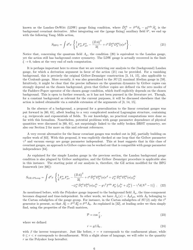
find, using the properties of the Pauli matrices,
P = cosr
2, (23)
where we definedr = gβA0 , (24)
with β the inverse temperature. Just like before, r = π corresponds to the confinement phase, while0 ≤ r < π corresponds to deconfinement. With a slight abuse of language, we will refer to the quantityr as the Polyakov loop hereafter.
6
Since the scope of this work is limited to one-loop order, only terms quadratic in the quantum fields inthe action (22) shall be considered. One then immediately gets an action that can be split in term comingfrom the two color sectors: the 3rd color direction, called Cartan direction, which does not depend onthe parameter r; and one coming from the 2 × 2 block given by the 1st and 2nd color directions. Thissecond 2× 2 color sector is orthogonal to the Cartan direction and does depend on r. The scenario canthen be seen as a system where the vector field has an imaginary chemical potential irT and has isospins+1 and −1 related to the 2× 2 color sector and one isospin 0 related to the 1× 1 color sector.
4 The finite temperature effective action at leading order
Considering only the quadratic terms of (22), the integration of the partition function gives us thefollowing vacuum energy at one-loop order, defined according to (13),
βV Ev = −d(N2 − 1)
2Ng2λ4 +
1
2(d− 1) tr ln
D4 + λ4
−D2− 1
2tr ln(−D2) , (25)
where V is now just the spacial volume. Here, D is the covariant derivative in the adjoint representationin the presence of the background A3
0 field and λ4 = 2Ng2γ4. Throughout this work, it is always tacitlyassumed we are working with N = 2 colors, although we will frequently continue to explicitly write Ndependence for generality. Using the usual Matsubara formalism, we have that D2 = (2πnT +rsT )2 +~q2,where n is the Matsubara mode, ~q is the spacelike momentum component, and s is the isospin, given by−1, 0, or +1 for the SU(2) case3.
The general trace is of the form
1
βVtr ln(−D2 +m2) = T
∑s
+∞∑n=−∞
∫d3−εq
(2π)3−ε ln((2πnT + rsT )2 + ~q2 +m2
), (26)
which will be computed immediately below.
4.1 The sum-integral: 2 different computations
We want to compute the following expression:
I = T
+∞∑n=−∞
∫d3−εq
(2π)3−ε ln((2πnT + rT )2 + ~q2 +m2
). (27)
One way to proceed is to start by deriving the previous expression with respect to m2. Then, one canuse the well-known formula from complex analysis
+∞∑n=−∞
f(n) = −π∑z0
Resz=z0
cot(πz)f(z) (28)
where the sum is over the poles z0 of the function f(z). Subsequently we integrate with respect to m2
(and determine the integration constant by matching the result with the known T = 0 case). Finally onecan split off the analogous T = 0 trace (which does not depend on the background field) to find
I =
∫d4−εq
(2π)4−ε ln(q2 +m2) + T
∫d3q
(2π)3ln
(1 + e−2
√~q2+m2
T − 2e−√~q2+m2
T cos r
). (29)
where the limit ε → 0 was taken in the (convergent) second integral. The first term in the r.h.s. is the(divergent) zero temperature contribution.
3The SU(3) case was handled in [32] as well (see also [67]).
7
Another way to compute the above integral is by making use of Zeta function regularization techniques,which are particularly useful in the computation of the Casimir energy in various configurations see[68, 69]. The advantage of this second technique is that, although it is less direct, it provides one with aneasy way to analyze the high and low temperature limits as well as the small mass limit, as we will nowshow. Moreover, within this framework, the regularization procedures are often quite transparent. Onestarts by writing the logarithm as lnx = − lims→0 ∂sx
−s, after which the integral over the momenta canbe performed:
I = −T lims→0
∂s
(µ2s
∞∑n=−∞
Γ(s− 3/2)
8π32 Γ(s)
[(2πnT + rT )2 +m2
] 32−s), (30)
where the renormalization scale µ has been introduced to get dimensional agreement for s 6= 0, and wherewe already put ε = 0, as s will function as a regulator — i.e. we assume s > 3/2 and analytically continuateto bring s → 0. Using the integral representation of the Gamma function, the previous expression canbe recast to
I = −T lims→0
∂s
(µ2s
∞∑n=−∞
1
8π32 Γ(s)
∫ ∞0
ts−5/2e−t((2πnT+rT )2+m2)dt
)
= − lims→0
∂s
(µ2s T 4−2s
4sπ2s−3/2Γ(s)
∫ ∞0
dyys−5/2e−m2y
4π2T2
∞∑n=−∞
e−y(n+ r2π )2
), (31)
where the variable of integration was transformed as y = 4π2T 2t ≥ 0 in the second line. Using thePoisson rule (valid for positive ω):
+∞∑n=−∞
e−(n+x)2ω =
√π
ω
(1 + 2
∞∑n=1
e−n2π2
ω cos (2nπx)
), (32)
we obtain that
I = − lims→0
∂sµ2s
[Γ(s− 2)T 4−2s
4sπ2s−2Γ(s)
(m2
4π2T 2
)2−s
+
T 4−2s
4s−1πsΓ(s)
(m2
4π2T 2
)1−s/2 ∞∑n=1
ns−2 cos (nr)K2−s
(nmT
)], (33)
where Kν(z) is the modified Bessel function of the second kind. Simplifying this, we find
I =m4
2(4π)2
[ln
(m2
µ2
)− 3
2
]−∞∑n=1
m2T 2 cos (nr)
π2n2K2
(nmT
), (34)
where the first term is the T = 0 contribution, and the sum is the finite-temperature correction. Usingnumerical integration and series summation, it can be checked that both results (29) and (34) are indeedidentical. Throughout this paper, we will mostly base ourselves on the expression (29). Nonetheless theBessel series is quite useful in obtaining the limit cases m = 0, T → ∞, and T → 0 by means of thecorresponding behaviour of K2(z). Observing that
limm→0
(−m2T 2K2
(mnT
)cos(nrs)
π2n2
)= −2T 4 cos(nrs)
π2n4, (35)
we obtain
Im=0 = −T4
π2
[Li4(e−irs
)+ Li4
(eirs)], (36)
where Lis(z) =∑∞n=1
zn
ns is the polylogarithm or Jonquière’s function.
Analogously,
limT→∞
K2
(mnT
)∼ 2T 2
m2n2− 1
2,
8

so that
IT→∞ =m4
2(4π)2
[ln
(m2
µ2
)− 3
2
]+
T 2
4π2
m2[Li2(e−irs
)+ Li2
(eirs)]− 4T 2
[Li4(e−irs
)+ Li4
(eirs)]
.
(37)Finally for T → 0 we can use the asymptotic expansion of the Bessel function [70]:
Kν(z) ∼√
π
2ze−z
( ∞∑k=0
ak(ν)
zk
), |Arg(z)| ≤ 3
2π , (38)
where ak(ν) are finite factors. So, at first order (k = 0),
IT→0 =m4
2(4π)2
[ln
(m2
µ2
)− 3
2
]− m3/2T 5/2
2√
2π3/2
[Li 5
2
(e−
mT −irs
)+ Li 5
2
(e−
mT +irs
)]. (39)
4.2 The result for further usage
Making use of the result (29) we may define
I(m2, r, s, T ) = T
∫d3q
(2π)3ln
(1 + e−2
√~q2+m2
T − 2e−√~q2+m2
T cos rs
), (40)
so that the vacuum energy (25) can be rewritten as
Ev =− d(N2 − 1)
2Ng2λ4 +
1
2(d− 1)(N2 − 1) trT=0 ln
∂4 + λ4
−∂2− 1
2(N2 − 1) trT=0 ln(−∂2)
+∑s
(1
2(d− 1)(I(iλ2, r, s, T ) + I(−iλ2, r, s, T )− I(0, r, s, T ))− 1
2I(0, r, s, T )
),
(41)
where trT=0 denotes the trace taken at zero temperature.
5 Minimization of the effective action, the Polyakov loop andthe Gribov mass
5.1 Warming-up exercise: assuming a T -independent Gribov mass λ
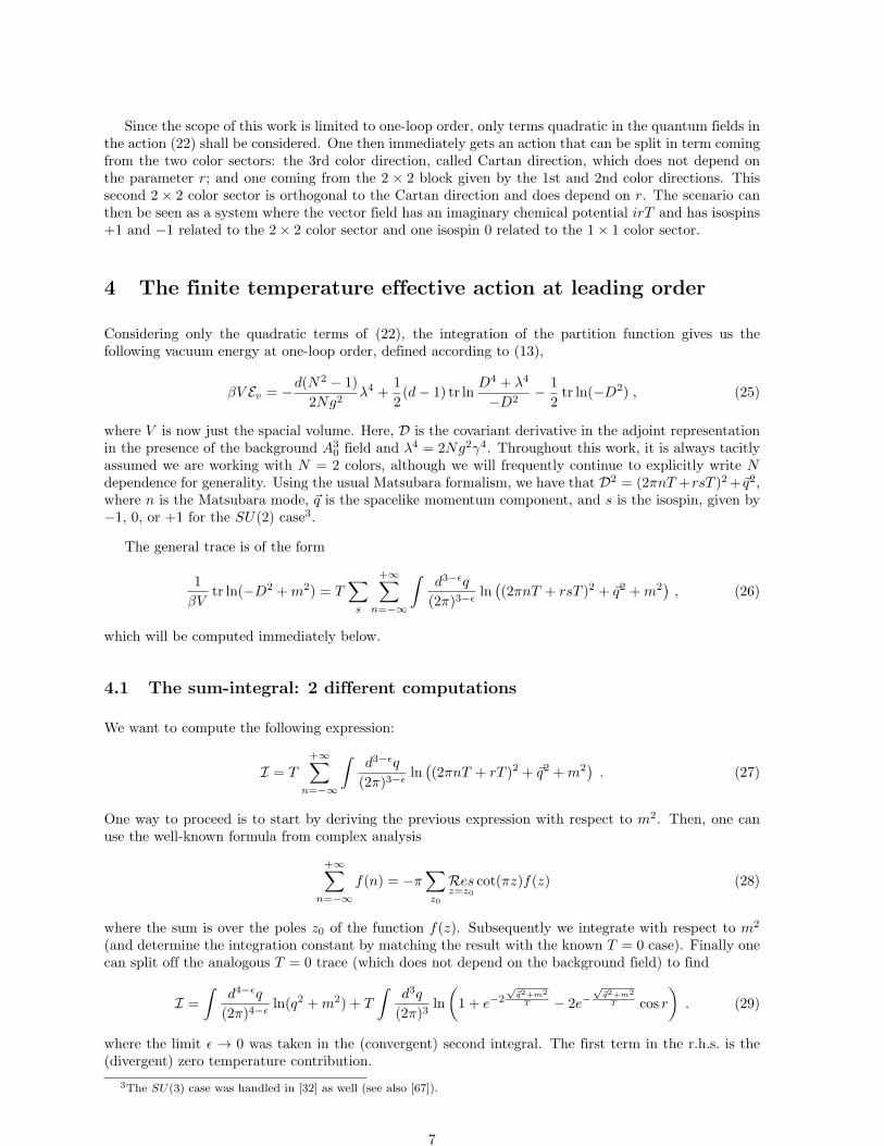
As a first simpler case, let us simplify matters slightly by assuming that the temperature does notinfluence the Gribov parameter λ. This means that λ will be supposed to assume its zero-temperaturevalue, which we will call λ0, given by the solution of the gap equation (7) at zero temperature. In thiscase, only the terms with the function I matter in (41), since the other terms do not explicitely dependon the Polyakov line r. Plotting this part of the potential (see Figure 1), one finds by visual inspectionthat a second-order phase transition occurs from the minimum with r = π to a minimum with r 6= π.The transition can be identified by the condition
d2
dr2Ev∣∣∣∣r=π
= 0 . (42)
Using the fact that
∂2I
∂r2(m2, r = π, s, T ) = −2T
∫d3q
(2π)3
e−√~q2+m2
T(1 + e−
√~q2+m2
T
)2 (43)
when s = ±1 and zero when s = 0, the equation (42) can be straightforwardly solved numerically for thecritical temperature. We find
Tcrit = 0.45λ0 . (44)
9
0.5 1.0 1.5 2.0 2.5 3.0r
0.005
0.010
0.015
0.020
@EvHTL-EvHT=0LDΛ04
Figure 1: The effective potential (41) at the temperatures (from below upwards at r = π) 0.42, 0.44, 0.46,and 0.48 times λ as a function of r, with the simplifying assumption that λ maintains its zero-temperaturevalue λ0 throughout. It can be seen that the minimum of the potential moves away from r = π in betweenT = 0.44λ and 0.46λ.
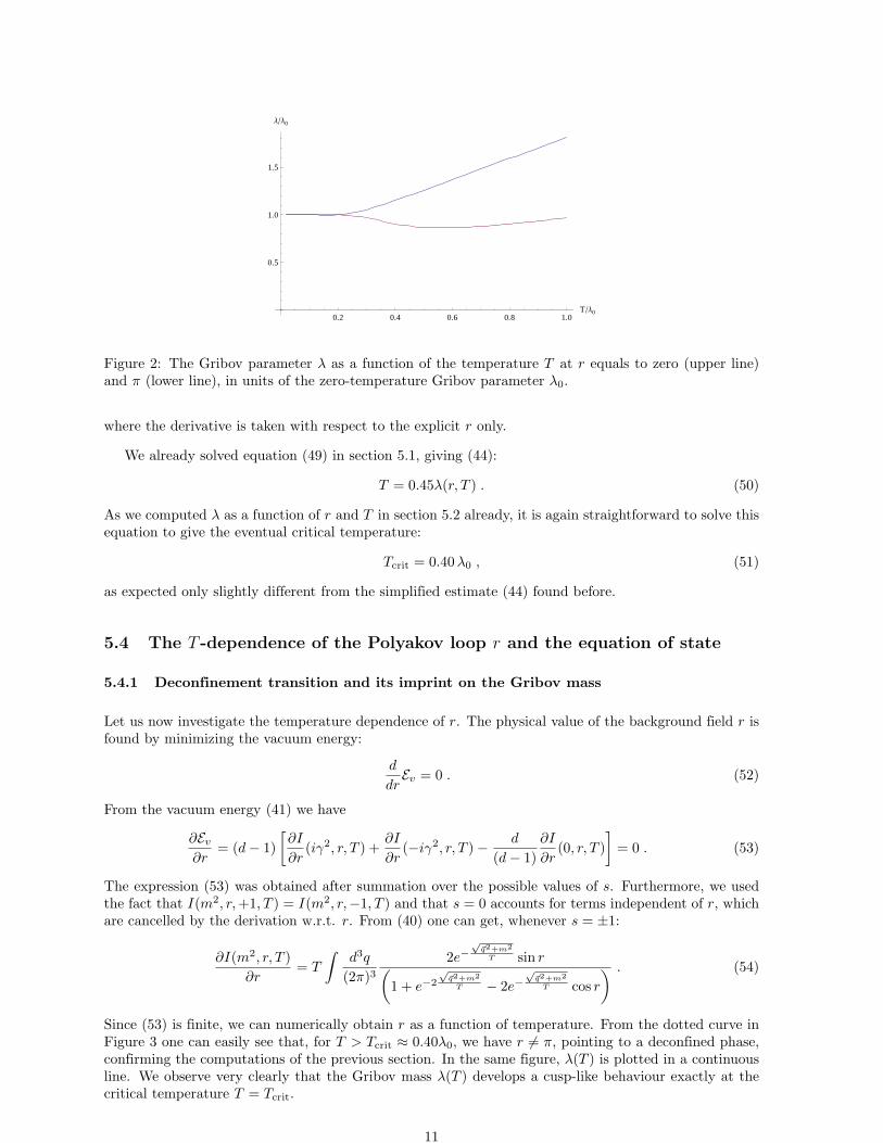
5.2 The T -dependence of the Gribov mass λ
Let us now investigate what happens to the Gribov parameter λ when the temperature is nonzero. Takingthe derivative of the effective potential (41) with respect to λ2 and dividing by d(N2 − 1)λ2/Ng2 (as weare not interested in the solution λ2 = 0) yields the gap equation for general number of colors N :
1 =1
2
d− 1
dNg2 tr
1
∂4 + λ4+
1
2
d− 1
d
Ng2
N2 − 1
i
λ2
∑s
(∂I
∂m2(iλ2, r, s, T )− ∂I
∂m2(−iλ2, r, s, T )
), (45)
where the notation ∂I/∂m2 denotes the derivative of I with respect to its first argument (written m2 in(40)). If we now define λ0 to be the solution to the gap equation at T = 0:
1 =1
2
d− 1
dNg2 tr
1
∂4 + λ40
, (46)
then we can subtract this equation from the general gap equation (45). After dividing through (d −1)Ng2/2d and setting d = 4 and N = 2, the result is∫
d4q
(2π)4
(1
q4 + λ4− 1
q4 + λ40
)+
i
3λ2
∑s
(∂I
∂m2(iλ2, r, s, T )− ∂I
∂m2(−iλ2, r, s, T )
)= 0 , (47)
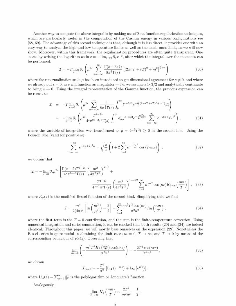
where now all integrations are convergent. This equation can be easily solved numerically to yield λ asa function of temperature T and background r, in units λ0. This is shown in Figure 2.
5.3 Absolute minimum of the effective action
As λ does not change much when including its dependence on temperature and background, the transitionis still second order and its temperature is, therefore, still given by the condition (42). Now, however,the potential depends explicitely on r, but also implicitely due to the presence of the r-dependent λ. Wetherefore have
d2
dr2Ev∣∣∣∣r=π
=∂2Ev∂r2
+ 2dλ
dr
∂2Ev∂r∂λ
+d2λ
dr2
∂Ev∂λ
+
(dλ
dr
)2∂2Ev∂λ2
∣∣∣∣∣λ=λ(r),r=π
. (48)
Now, dλ/dr|r=π = 0 due to the symmetry at that point. Furthermore, as we are considering λ 6= 0,∂Ev/∂λ = 0 is the gap equation and is solved by λ(r). Therefore, we find for the condition of thetransition:
∂2Ev∂r2
(r, λ, T )
∣∣∣∣r=π
= 0 , (49)
10
0.2 0.4 0.6 0.8 1.0TΛ0
0.5
1.0
1.5
ΛΛ0
Figure 2: The Gribov parameter λ as a function of the temperature T at r equals to zero (upper line)and π (lower line), in units of the zero-temperature Gribov parameter λ0.
where the derivative is taken with respect to the explicit r only.
We already solved equation (49) in section 5.1, giving (44):
T = 0.45λ(r, T ) . (50)
As we computed λ as a function of r and T in section 5.2 already, it is again straightforward to solve thisequation to give the eventual critical temperature:
Tcrit = 0.40λ0 , (51)
as expected only slightly different from the simplified estimate (44) found before.
5.4 The T -dependence of the Polyakov loop r and the equation of state
5.4.1 Deconfinement transition and its imprint on the Gribov mass
Let us now investigate the temperature dependence of r. The physical value of the background field r isfound by minimizing the vacuum energy:
d
drEv = 0 . (52)
From the vacuum energy (41) we have
∂Ev∂r
= (d− 1)
[∂I
∂r(iγ2, r, T ) +
∂I
∂r(−iγ2, r, T )− d
(d− 1)
∂I
∂r(0, r, T )
]= 0 . (53)
The expression (53) was obtained after summation over the possible values of s. Furthermore, we usedthe fact that I(m2, r,+1, T ) = I(m2, r,−1, T ) and that s = 0 accounts for terms independent of r, whichare cancelled by the derivation w.r.t. r. From (40) one can get, whenever s = ±1:
∂I(m2, r, T )
∂r= T
∫d3q
(2π)3
2e−√~q2+m2
T sin r(1 + e−2
√~q2+m2
T − 2e−√~q2+m2
T cos r
) . (54)
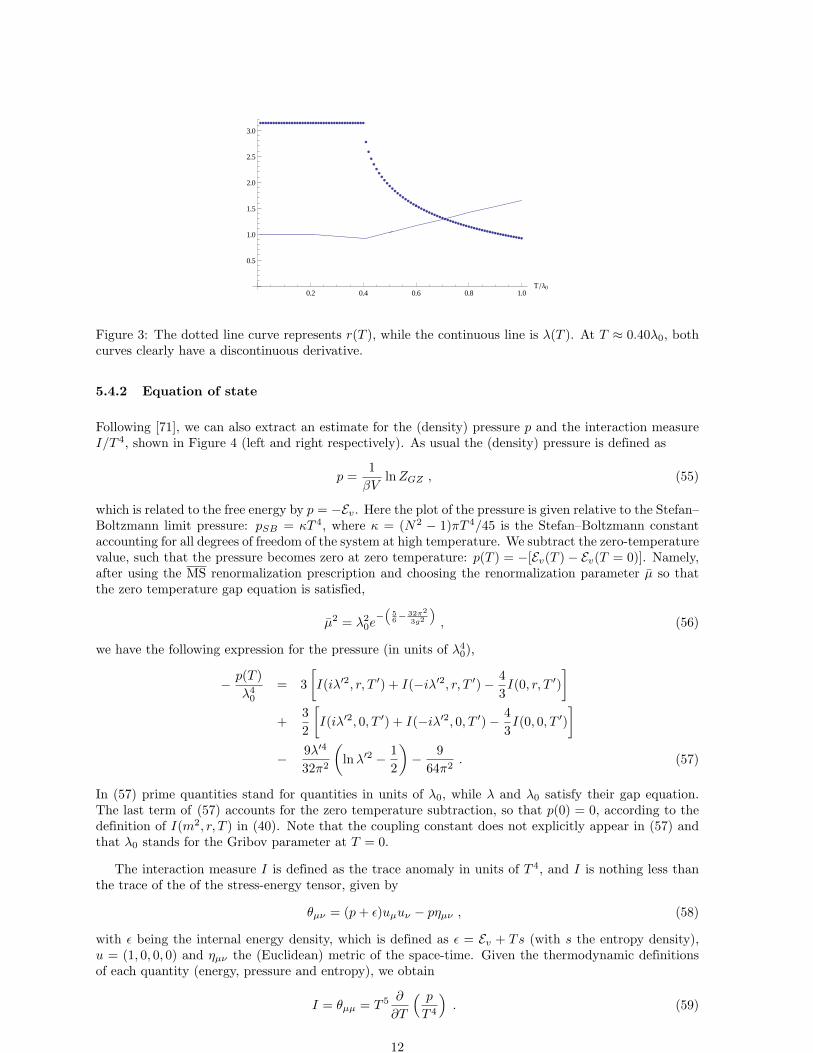
Since (53) is finite, we can numerically obtain r as a function of temperature. From the dotted curve inFigure 3 one can easily see that, for T > Tcrit ≈ 0.40λ0, we have r 6= π, pointing to a deconfined phase,confirming the computations of the previous section. In the same figure, λ(T ) is plotted in a continuousline. We observe very clearly that the Gribov mass λ(T ) develops a cusp-like behaviour exactly at thecritical temperature T = Tcrit.
11
0.2 0.4 0.6 0.8 1.0T Λ0
0.5
1.0
1.5
2.0
2.5
3.0
Figure 3: The dotted line curve represents r(T ), while the continuous line is λ(T ). At T ≈ 0.40λ0, bothcurves clearly have a discontinuous derivative.
5.4.2 Equation of state
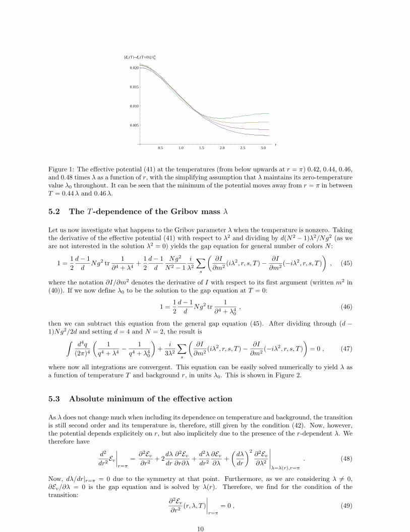
Following [71], we can also extract an estimate for the (density) pressure p and the interaction measureI/T 4, shown in Figure 4 (left and right respectively). As usual the (density) pressure is defined as
p =1
βVlnZGZ , (55)
which is related to the free energy by p = −Ev. Here the plot of the pressure is given relative to the Stefan–Boltzmann limit pressure: pSB = κT 4, where κ = (N2 − 1)πT 4/45 is the Stefan–Boltzmann constantaccounting for all degrees of freedom of the system at high temperature. We subtract the zero-temperaturevalue, such that the pressure becomes zero at zero temperature: p(T ) = −[Ev(T )− Ev(T = 0)]. Namely,after using the MS renormalization prescription and choosing the renormalization parameter µ so thatthe zero temperature gap equation is satisfied,
µ2 = λ20e−(
56−
32π2
3g2
), (56)
we have the following expression for the pressure (in units of λ40),
− p(T )
λ40
= 3
[I(iλ′2, r, T ′) + I(−iλ′2, r, T ′)− 4
3I(0, r, T ′)
]+
3
2
[I(iλ′2, 0, T ′) + I(−iλ′2, 0, T ′)− 4
3I(0, 0, T ′)
]− 9λ′4
32π2
(lnλ′2 − 1
2
)− 9
64π2. (57)
In (57) prime quantities stand for quantities in units of λ0, while λ and λ0 satisfy their gap equation.The last term of (57) accounts for the zero temperature subtraction, so that p(0) = 0, according to thedefinition of I(m2, r, T ) in (40). Note that the coupling constant does not explicitly appear in (57) andthat λ0 stands for the Gribov parameter at T = 0.
The interaction measure I is defined as the trace anomaly in units of T 4, and I is nothing less thanthe trace of the of the stress-energy tensor, given by
θµν = (p+ ε)uµuν − pηµν , (58)
with ε being the internal energy density, which is defined as ε = Ev + Ts (with s the entropy density),u = (1, 0, 0, 0) and ηµν the (Euclidean) metric of the space-time. Given the thermodynamic definitionsof each quantity (energy, pressure and entropy), we obtain
I = θµµ = T 5 ∂
∂T
( p
T 4
). (59)
12
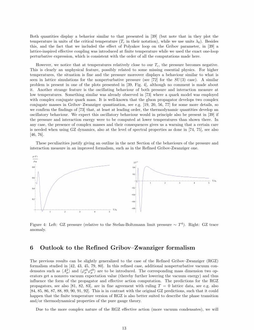
Both quantities display a behavior similar to that presented in [39] (but note that in they plot thetemperature in units of the critical temperature (Tc in their notation), while we use units λ0). Besidesthis, and the fact that we included the effect of Polyakov loop on the Gribov parameter, in [39] alattice-inspired effective coupling was introduced at finite temperature while we used the exact one-loopperturbative expression, which is consistent with the order of all the computations made here.
However, we notice that at temperatures relatively close to our Tc, the pressure becomes negative.This is clearly an unphysical feature, possibly related to some missing essential physics. For highertemperatures, the situation is fine and the pressure moreover displays a behaviour similar to what isseen in lattice simulations for the nonperturbative pressure (see [72] for the SU(3) case). A similarproblem is present in one of the plots presented in [39, Fig. 4], although no comment is made aboutit. Another strange feature is the oscillating behaviour of both pressure and interaction measure atlow temperatures. Something similar was already observed in [73] where a quark model was employedwith complex conjugate quark mass. It is well-known that the gluon propagator develops two complexconjugate masses in Gribov–Zwanziger quantization, see e.g. [19, 20, 56, 77] for some more details, sowe confirm the findings of [73] that, at least at leading order, the thermodynamic quantities develop anoscillatory behaviour. We expect this oscillatory behaviour would in principle also be present in [39] ifthe pressure and interaction energy were to be computed at lower temperatures than shown there. Inany case, the presence of complex masses and their consequences gives us a warning that a certain careis needed when using GZ dynamics, also at the level of spectral properties as done in [74, 75], see also[46, 76].
These peculiarities justify giving an outline in the next Section of the behaviours of the pressure andinteraction measure in an improved formalism, such as in the Refined Gribov-Zwanziger one.
1 2 3 4 5T Λ0
0.2
0.4
0.6
0.8
p HT L
pSB
1 2 3 4 5T Λ0
-0.8
-0.6
-0.4
-0.2
0.2
0.4
IT 4
Figure 4: Left: GZ pressure (relative to the Stefan-Boltzmann limit pressure ∼ T 4). Right: GZ traceanomaly.
6 Outlook to the Refined Gribov–Zwanziger formalism
The previous results can be slightly generalized to the case of the Refined Gribov–Zwanziger (RGZ)formalism studied in [42, 43, 45, 79, 80]. In this refined case, additional nonperturbative vacuum con-densates such as 〈A2
µ〉 and 〈ϕabµ ϕabµ 〉 are to be introduced. The corresponding mass dimension two op-erators get a nonzero vacuum expectation value (thereby further lowering the vacuum energy) and thusinfluence the form of the propagator and effective action computation. The predictions for the RGZpropagators, see also [81, 82, 83], are in fine agreement with ruling T = 0 lattice data, see e.g. also[84, 85, 86, 87, 88, 89, 90, 91, 92]. This is in contrast with the original GZ predictions, such that it couldhappen that the finite temperature version of RGZ is also better suited to describe the phase transitionand/or thermodynamical properties of the pure gauge theory.
Due to the more complex nature of the RGZ effective action (more vacuum condensates), we will
13
relegate a detailed (variational) analysis of their finite temperature counterparts4 to future work, as thiswill require new tools. Here, we only wish to present a first estimate of the deconfinement critical tem-perature Tc using as input the T = 0 RGZ gluon propagator where the nonperturbative mass parametersare fitted to lattice data for the same propagator. More precisely, we use [77]
∆abµν(p) = δab
p2 +M2 + ρ1
p4 + p2(M2 +m2 + ρ1) +m2(M2 + ρ1) + λ4
(δµν −
pµpνp2
). (60)
where we omitted the global normalization factor Z which drops out from our leading order computation5.In this expression, we have that
〈AaµAaµ〉 → −m2 , 〈ϕabµ ϕabµ 〉 →M2 ,1
2〈ϕabµ ϕabµ + ϕabµ ϕ
abµ 〉 → ρ1 . (61)
The free energy associated to the RGZ framework can be obtained by following the same steps as insection 4, leading to
Ev(T ) = (d− 1)
[I(r2
+, r, T ) + I(r2−, r, T )− I(N2, r, T )− 1
d− 1I(0, r, T )
]+
(d− 1)
2
[I(r2
+, 0, T ) + I(r2−, 0, T )− I(N2, 0, T )− 1
d− 1I(0, 0, T )
]+
∫ddp
(2π)dln
(p4 + (m2 +N2)p2 + (m2N2 + λ4)
p2 +N2
)− 3λ4d
4g2, (62)
with r2± standing for minus the roots of the denominator of the gluon propagator (60), N2 = M2 + ρ1,
and I(m2, r, T ) given by (40). Explicitly, the roots are
r2± =
(m2 +N2)±√
(m2 +N2)2 − 4(m2N2 + λ4)
2. (63)
The (central) condensate values were extracted from [77]:
N2 = M2 + ρ1 = 2.51 GeV2 , (64a)
m2 = −1.92 GeV2 , (64b)
λ4 = 5.3 GeV4 . (64c)
Once again the vacuum energy will be minimized with respect to the Polyakov loop expectation valuer. For the analysis of thermodynamic quantities, only contributions coming from terms proportional toI(m2, r, T ) will be needed. Therefore, we will always consider the difference Ev(T ) − Ev(T = 0). Sincein the present (RGZ) prescription the condensates are given by the zero temperature lattice results (64)instead of satisfying gap equations, the divergent contributions to the free energy are subtracted, and nospecific choice of renormalization scheme is needed. Furthermore, explicit dependence on the couplingconstant seems to drop out of the one-loop expression, such that no renormalization scale has to be chosen.Following the steps taken in Section 5.1, we find a second order phase transition at the temperature:
Tcrit = 0.25 GeV , (65)
which is not that far from the value of the SU(2) deconfinement temperature found on the lattice:Tc ≈ 0.295 GeV, as quoted in [96, 97].
In future work, it would in particular be interesting to find out whether —upon using the RGZformalism— the Gribov mass and/or RGZ condensates directly feel the deconfinement transition, similarto the cusp we discovered in the Gribov parameter following the exploratory restricted analysis of thispaper. This might also allow to shed further light on the ongoing discussion of whether the deconfinementtransition should be felt at the level of the correlation functions, in particular the electric screening massassociated with the longitudinal gluon propagator [98, 99, 100, 101].
4From [93, 94, 95], the nontrivial response of the d = 2 condensate 〈A2〉 to temperature already became clear.5This Z is related to the choice of a MOM renormalization scheme, the kind of scheme that can also be applied to lattice
Green functions, in contrast with the MS scheme.
14
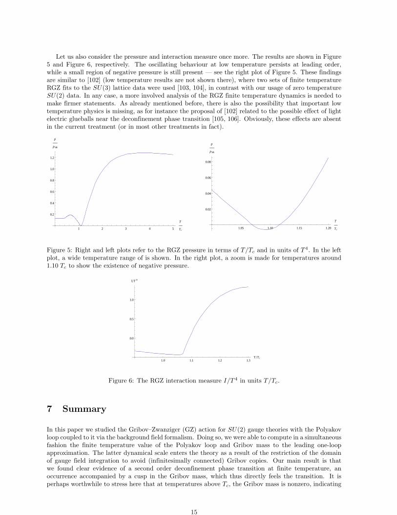
Let us also consider the pressure and interaction measure once more. The results are shown in Figure5 and Figure 6, respectively. The oscillating behaviour at low temperature persists at leading order,while a small region of negative pressure is still present — see the right plot of Figure 5. These findingsare similar to [102] (low temperature results are not shown there), where two sets of finite temperatureRGZ fits to the SU(3) lattice data were used [103, 104], in contrast with our usage of zero temperatureSU(2) data. In any case, a more involved analysis of the RGZ finite temperature dynamics is needed tomake firmer statements. As already mentioned before, there is also the possibility that important lowtemperature physics is missing, as for instance the proposal of [102] related to the possible effect of lightelectric glueballs near the deconfinement phase transition [105, 106]. Obviously, these effects are absentin the current treatment (or in most other treatments in fact).
1 2 3 4 5
T
Tc
0.2
0.4
0.6
0.8
1.0
1.2
p
pSB
1.05 1.10 1.15 1.20
T
Tc
0.02
0.04
0.06
0.08
p
pSB
Figure 5: Right and left plots refer to the RGZ pressure in terms of T/Tc and in units of T 4. In the leftplot, a wide temperature range of is shown. In the right plot, a zoom is made for temperatures around1.10 Tc to show the existence of negative pressure.
1.0 1.1 1.2 1.3T Tc
0.0
0.5
1.0
IT 4
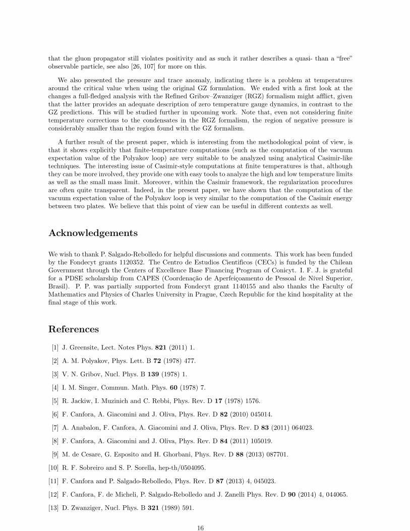
Figure 6: The RGZ interaction measure I/T 4 in units T/Tc.
7 Summary
In this paper we studied the Gribov–Zwanziger (GZ) action for SU(2) gauge theories with the Polyakovloop coupled to it via the background field formalism. Doing so, we were able to compute in a simultaneousfashion the finite temperature value of the Polyakov loop and Gribov mass to the leading one-loopapproximation. The latter dynamical scale enters the theory as a result of the restriction of the domainof gauge field integration to avoid (infinitesimally connected) Gribov copies. Our main result is thatwe found clear evidence of a second order deconfinement phase transition at finite temperature, anoccurrence accompanied by a cusp in the Gribov mass, which thus directly feels the transition. It isperhaps worthwhile to stress here that at temperatures above Tc, the Gribov mass is nonzero, indicating
15
that the gluon propagator still violates positivity and as such it rather describes a quasi- than a “free”observable particle, see also [26, 107] for more on this.
We also presented the pressure and trace anomaly, indicating there is a problem at temperaturesaround the critical value when using the original GZ formulation. We ended with a first look at thechanges a full-fledged analysis with the Refined Gribov–Zwanziger (RGZ) formalism might afflict, giventhat the latter provides an adequate description of zero temperature gauge dynamics, in contrast to theGZ predictions. This will be studied further in upcoming work. Note that, even not considering finitetemperature corrections to the condensates in the RGZ formalism, the region of negative pressure isconsiderably smaller than the region found with the GZ formalism.
A further result of the present paper, which is interesting from the methodological point of view, isthat it shows explicitly that finite-temperature computations (such as the computation of the vacuumexpectation value of the Polyakov loop) are very suitable to be analyzed using analytical Casimir-liketechniques. The interesting issue of Casimir-style computations at finite temperatures is that, althoughthey can be more involved, they provide one with easy tools to analyze the high and low temperature limitsas well as the small mass limit. Moreover, within the Casimir framework, the regularization proceduresare often quite transparent. Indeed, in the present paper, we have shown that the computation of thevacuum expectation value of the Polyakov loop is very similar to the computation of the Casimir energybetween two plates. We believe that this point of view can be useful in different contexts as well.
Acknowledgements
We wish to thank P. Salgado-Rebolledo for helpful discussions and comments. This work has been fundedby the Fondecyt grants 1120352. The Centro de Estudios Cientificos (CECs) is funded by the ChileanGovernment through the Centers of Excellence Base Financing Program of Conicyt. I. F. J. is gratefulfor a PDSE scholarship from CAPES (Coordenacão de Aperfeicoamento de Pessoal de Nível Superior,Brasil). P. P. was partially supported from Fondecyt grant 1140155 and also thanks the Faculty ofMathematics and Physics of Charles University in Prague, Czech Republic for the kind hospitality at thefinal stage of this work.
References
[1] J. Greensite, Lect. Notes Phys. 821 (2011) 1.
[2] A. M. Polyakov, Phys. Lett. B 72 (1978) 477.
[3] V. N. Gribov, Nucl. Phys. B 139 (1978) 1.
[4] I. M. Singer, Commun. Math. Phys. 60 (1978) 7.
[5] R. Jackiw, I. Muzinich and C. Rebbi, Phys. Rev. D 17 (1978) 1576.
[6] F. Canfora, A. Giacomini and J. Oliva, Phys. Rev. D 82 (2010) 045014.
[7] A. Anabalon, F. Canfora, A. Giacomini and J. Oliva, Phys. Rev. D 83 (2011) 064023.
[8] F. Canfora, A. Giacomini and J. Oliva, Phys. Rev. D 84 (2011) 105019.
[9] M. de Cesare, G. Esposito and H. Ghorbani, Phys. Rev. D 88 (2013) 087701.
[10] R. F. Sobreiro and S. P. Sorella, hep-th/0504095.
[11] F. Canfora and P. Salgado-Rebolledo, Phys. Rev. D 87 (2013) 4, 045023.
[12] F. Canfora, F. de Micheli, P. Salgado-Rebolledo and J. Zanelli Phys. Rev. D 90 (2014) 4, 044065.
[13] D. Zwanziger, Nucl. Phys. B 321 (1989) 591.
16
[14] D. Zwanziger, Nucl. Phys. B 323 (1989) 513.
[15] D. Zwanziger, Nucl. Phys. B 399 (1993) 477.
[16] G. Dell’Antonio and D. Zwanziger, Nucl. Phys. B 326 (1989) 333.
[17] G. Dell’Antonio and D. Zwanziger, Commun. Math. Phys. 138 (1991) 291.
[18] P. van Baal, Nucl. Phys. B 369 (1992) 259.
[19] D. Dudal, M. S. Guimaraes and S. P. Sorella, Phys. Rev. Lett. 106 (2011) 062003.
[20] D. Dudal, M. S. Guimaraes and S. P. Sorella, Phys. Lett. B 732 (2014) 247.
[21] F. Canfora and L. Rosa, Phys. Rev. D 88 (2013) 045025.
[22] F. Canfora, P. Pais and P. Salgado-Rebolledo, Eur. Phys. J. C 74 (2014) 2855.
[23] M. A. L. Capri, D. Dudal, A. J. Gomez, M. S. Guimaraes, I. F. Justo, S. P. Sorella and D. Ver-cauteren, Phys. Rev. D 88 (2013) 085022.
[24] M. A. L. Capri, D. Dudal, A. J. Gomez, M. S. Guimaraes, I. F. Justo and S. P. Sorella, Eur. Phys.J. C 73 (2013) 3, 2346.
[25] F. Canfora, A. J. Gomez, S. P. Sorella and D. Vercauteren, Annals Phys. 345 (2014) 166.
[26] A. Maas, Phys. Rept. 524 (2013) 203.
[27] J. Braun, H. Gies and J. M. Pawlowski, Phys. Lett. B 684 (2010) 262.
[28] F. Marhauser and J. M. Pawlowski, arXiv:0812.1144 [hep-ph].
[29] H. Reinhardt and J. Heffner, Phys. Lett. B 718 (2012) 672.
[30] H. Reinhardt and J. Heffner, Phys. Rev. D 88 (2013) 4, 045024.
[31] J. Heffner and H. Reinhardt, Phys. Rev. D 91 (2015) 085022.
[32] U. Reinosa, J. Serreau, M. Tissier and N. Wschebor, Phys. Lett. B 742 (2015) 61.
[33] U. Reinosa, J. Serreau, M. Tissier and N. Wschebor, Phys. Rev. D 91 (2015) 4, 045035.
[34] C. S. Fischer and J. A. Mueller, Phys. Rev. D 80 (2009) 074029.
[35] T. K. Herbst, M. Mitter, J. M. Pawlowski, B. J. Schaefer and R. Stiele, Phys. Lett. B 731 (2014)248.
[36] A. Bender, D. Blaschke, Y. Kalinovsky and C. D. Roberts, Phys. Rev. Lett. 77 (1996) 3724.
[37] D. Zwanziger, Phys. Rev. D 76 (2007) 125014.
[38] K. Lichtenegger and D. Zwanziger, Phys. Rev. D 78 (2008) 034038.
[39] K. Fukushima and N. Su, Phys. Rev. D 88 (2013) 076008.
[40] M. A. L. Capri, D. Dudal, M. S. Guimaraes, L. F. Palhares and S. P. Sorella, Phys. Lett. B 719(2013) 448.
[41] N. Maggiore and M. Schaden, Phys. Rev. D 50 (1994) 6616.
[42] D. Dudal, S. P. Sorella, N. Vandersickel and H. Verschelde, Phys. Rev. D 77 (2008) 071501.
[43] D. Dudal, J. A. Gracey, S. P. Sorella, N. Vandersickel and H. Verschelde, Phys. Rev. D 78 (2008)065047.
[44] D. Dudal, S. P. Sorella and N. Vandersickel, Eur. Phys. J. C 68 (2010) 283.
[45] D. Dudal, S. P. Sorella and N. Vandersickel, Phys. Rev. D 84 (2011) 065039.
17
[46] L. Baulieu and S. P. Sorella, Phys. Lett. B 671 (2009) 481.
[47] D. Dudal, S. P. Sorella, N. Vandersickel and H. Verschelde, Phys. Rev. D 79 (2009) 121701.
[48] S. P. Sorella, Phys. Rev. D 80 (2009) 025013.
[49] S. P. Sorella, J. Phys. A 44 (2011) 135403.
[50] M. A. L. Capri, A. J. Gomez, M. S. Guimaraes, V. E. R. Lemes, S. P. Sorella and D. G. Tedesco,Phys. Rev. D 82 (2010) 105019.
[51] D. Dudal and S. P. Sorella, Phys. Rev. D 86 (2012) 045005.
[52] A. Reshetnyak, Int. J. Mod. Phys. A 29 (2014) 1450184.
[53] A. Cucchieri, D. Dudal, T. Mendes and N. Vandersickel, Phys. Rev. D 90 (2014) 5, 051501.
[54] M. A. L. Capri, M. S. Guimaraes, I. F. Justo, L. F. Palhares and S. P. Sorella, Phys. Rev. D 90(2014) 8, 085010.
[55] M. Schaden and D. Zwanziger, arXiv:1412.4823 [hep-ph].
[56] L. Baulieu, D. Dudal, M. S. Guimaraes, M. Q. Huber, S. P. Sorella, N. Vandersickel and D. Zwanziger,Phys. Rev. D 82 (2010) 025021.
[57] K. Fukushima, Phys. Lett. B 591 (2004) 277.
[58] C. Ratti, M. A. Thaler and W. Weise, Phys. Rev. D 73 (2006) 014019.
[59] S. Gongyo and H. Iida, Phys. Rev. D 89 (2014) 2, 025022.
[60] P. Lavrov, O. Lechtenfeld and A. Reshetnyak, JHEP 1110 (2011) 043.
[61] P. M. Lavrov and O. Lechtenfeld, Phys. Lett. B 725 (2013) 386.
[62] M. A. L. Capri, A. D. Pereira, R. F. Sobreiro and S. P. Sorella, arXiv:1505.05467 [hep-th].
[63] R. F. Sobreiro and S. P. Sorella, JHEP 0506 (2005) 054.
[64] M. A. L. Capri et al, work in progress.
[65] S. Weinberg, The quantum theory of fields. Vol. 2: Modern applications, Cambridge, UK: Univ. Pr.(1996).
[66] D. Zwanziger, Nucl. Phys. B 209 (1982) 336.
[67] J. Serreau, arXiv:1504.00038 [hep-th].
[68] E. Elizalde, Ten physical Applications of Spectral Zeta Functions, Springer, Berlin Heidelberg (1995).
[69] M. Bordag, G. L. Klimchitskaya, U. Mohideen and V. M. Mostepanenko, Advances in the CasimirEffect, Oxford University Press, Oxford New York (2010).
[70] M. Abramowitz and I. A. Stegun, Handbook of mathematical functions, National Bureau of Stan-dards, Applied Mathematics Series - 55 (1972).
[71] O. Philipsen, Prog. Part. Nucl. Phys. 70 (2013) 55.
[72] S. Borsanyi, G. Endrodi, Z. Fodor, S. D. Katz and K. K. Szabo, JHEP 1207 (2012) 056.
[73] S. Benic, D. Blaschke and M. Buballa, Phys. Rev. D 86 (2012) 074002.
[74] N. Su and K. Tywoniuk, arXiv:1409.3203 [hep-ph].
[75] W. Florkowski, R. Ryblewski, N. Su and K. Tywoniuk, arXiv:1504.03176 [hep-ph].
[76] D. Dudal and M. S. Guimaraes, Phys. Rev. D 83 (2011) 045013.
18
[77] A. Cucchieri, D. Dudal, T. Mendes and N. Vandersickel, Phys. Rev. D 85 (2012) 094513.
[78] J. A. Gracey, Phys. Lett. B 632 (2006) 282 [Erratum-ibid. 686 (2010) 319].
[79] J. A. Gracey, Phys. Rev. D 82 (2010) 085032 [arXiv:1009.3889 [hep-th]].
[80] D. J. Thelan and J. A. Gracey, Phys. Rev. D 89 (2014) 10, 107701.
[81] D. Dudal, O. Oliveira and N. Vandersickel, Phys. Rev. D 81 (2010) 074505.
[82] D. Dudal, O. Oliveira and J. Rodriguez-Quintero, Phys. Rev. D 86 (2012) 105005.
[83] O. Oliveira and P. J. Silva, Phys. Rev. D 86 (2012) 114513.
[84] I. L. Bogolubsky, E. M. Ilgenfritz, M. Muller-Preussker and A. Sternbeck, PoS LAT 2007 (2007)290.
[85] A. Cucchieri and T. Mendes, PoS LAT 2007 (2007) 297.
[86] A. Sternbeck, L. von Smekal, D. B. Leinweber and A. G. Williams, PoS LAT 2007 (2007) 340.
[87] A. Maas, Phys. Rev. D 79 (2009) 014505.
[88] O. Oliveira and P. J. Silva, Phys. Rev. D 79 (2009) 031501.
[89] A. Cucchieri and T. Mendes, Phys. Rev. D 78 (2008) 094503.
[90] A. Cucchieri, A. Maas and T. Mendes, Phys. Rev. D 77 (2008) 094510.
[91] A. Cucchieri and T. Mendes, Phys. Rev. Lett. 100 (2008) 241601.
[92] I. L. Bogolubsky, E. M. Ilgenfritz, M. Muller-Preussker and A. Sternbeck, Phys. Lett. B 676 (2009)69.
[93] M. N. Chernodub and E.-M. Ilgenfritz, Phys. Rev. D 78 (2008) 034036.
[94] D. Dudal, J. A. Gracey, N. Vandersickel, D. Vercauteren and H. Verschelde, Phys. Rev. D 80 (2009)065017.
[95] D. Vercauteren and H. Verschelde, Phys. Rev. D 82 (2010) 085026.
[96] A. Cucchieri, A. Maas and T. Mendes, Phys. Rev. D 75 (2007) 076003.
[97] J. Fingberg, U. M. Heller and F. Karsch, Nucl. Phys. B 392 (1993) 493.
[98] A. Maas, J. M. Pawlowski, L. von Smekal and D. Spielmann, Phys. Rev. D 85 (2012) 034037
[99] A. Cucchieri and T. Mendes, PoS LATTICE 2011 (2011) 206
[100] A. Cucchieri and T. Mendes, Acta Phys. Polon. Supp. 7 (2014) 3, 559.
[101] P. J. Silva, O. Oliveira, P. Bicudo and N. Cardoso, Phys. Rev. D 89 (2014) 7, 074503.
[102] K. Fukushima and K. Kashiwa, Phys. Lett. B 723 (2013) 360.
[103] R. Aouane, V. G. Bornyakov, E. M. Ilgenfritz, V. K. Mitrjushkin, M. Muller-Preussker and A. Stern-beck, Phys. Rev. D 85 (2012) 034501.
[104] R. Aouane, F. Burger, E.-M. Ilgenfritz, M. Muller-Preussker and A. Sternbeck, Phys. Rev. D 87(2013) 11, 114502.
[105] N. Ishii, H. Suganuma and H. Matsufuru, Phys. Rev. D 66 (2002) 014507.
[106] Y. Hatta and K. Fukushima, Phys. Rev. D 69 (2004) 097502.
[107] M. Haas, L. Fister and J. M. Pawlowski, Phys. Rev. D 90 (2014) 9, 091501.
19