Embed Size (px)
Citation preview
arX
iv:h
ep-p
h/97
1124
3v1
5 N
ov 1
997
Non-perturbative renormalization of QCD1
Rainer Sommer
DESY-IfH, Platanenallee 6, D-15738 Zeuthen
DESY 97-207
Abstract. In these lectures, we discuss different types of renormalization problemsin QCD and their non-perturbative solution in the framework of the lattice formula-tion. In particular the recursive finite size methods to compute the scale-dependence ofrenormalized quantities is explained. An important ingredient in the practical applica-tions is the Schrodinger functional. It is introduced and its renormalization propertiesare discussed.Concerning applications, the computation of the running coupling and the runningquark mass are covered in detail and it is shown how the Λ-parameter and renormal-ization group invariant quark mass can be obtained. Further topics are the renormal-ization of isovector currents and non-perturbative Symanzik improvement.
Contents
1. IntroductionBasic renormalization: hadron spectrum; Finite renormalization: (semi-)leptonicdecays; Scale dependent renormalization; Irrelevant operators
2. The problem of scale dependent renormalizationThe extraction of α from experiments; Reaching large scales in lattice QCD
3. The Schrodinger functionalDefinition; Quantum mechanical interpretation; Background field; Perturbative ex-pansion; General renormalization properties; Renormalized coupling; Quarks; Renor-malized mass; Lattice formulation
4. The computation of α(q)The step scaling function; Lattice spacing effects in perturbation theory; The con-tinuum limit – universality; The running of the coupling; The low energy scale;Matching at finite energy; The Λ parameter of quenched QCD; The use of barecouplings
5. Renormalization group invariant quark mass
6. Chiral symmetry, normalization of currents and O(a)-improvementChiral Ward identities; O(a)-improvement; Normalization of isovector currents
7. Summary, Conclusions
1 Introduction
The topic of these lectures is the computation of properties of particles that arebound by the strong interaction or more generally interact strongly. The strong
1 Lectures given at the 36. Internationale Universitatswochen fur Kern- und Teilchen-physik (Schladming 1997) : Computing Particles
2 Rainer Sommer
interactions are theoretically described by Quantum Chromo Dynamics (QCD),a local quantum field theory.
Starting from the Lagrangian of a field theory, predictions for cross sectionsand other observables are usually made by applying renormalized perturbationtheory, the expansion in terms of the (running) couplings of the theory. While thisexpansion is well controlled as far as electroweak interactions are concerned, itsapplication in QCD is limited to high energy processes where the QCD coupling,α, is sufficiently small. In general – and in particular for the calculation of boundstate properties – a non-perturbative solution of the theory is required.
The only method that is known to address this problem is the numericalsimulation of the Euclidean path integral of QCD on a space-time lattice. By“solution of the theory” we here mean that one poses a well defined question like“what is the value of the π decay constant”, and obtains the answer (within acertain precision) through a series of Monte Carlo (MC) simulations. This thenallows to test the agreement of theory and experiment on the one hand andhelps in the determination of Standard Model parameters from experiments onthe other hand.
Quantum field theories are defined by first formulating them in a regulariza-tion with an ultraviolet cutoff Λcut and then considering the limit Λcut → ∞. Inthe lattice formulation (Wilson 1974), the cutoff is given by the inverse of thelattice spacing a; we have to consider the continuum limit a → 0. At a finitevalue of a, the theory is defined in terms of the bare coupling constant, baremasses and bare fields. Before making predictions for experimental observables(or more generally for observables that have a well defined continuum limit) thecoupling, masses and fields have to be renormalized. This is the subject of mylectures.
Renormalization is an ultraviolet phenomenon with relevant momentum scalesof order a−1. Since α becomes weak in the ultraviolet, one expects to be ableto perform renormalizations perturbatively, i.e. computed in a power series inα as one approaches the continuum limit a → 0.2 However, one has to takecare about the following point. In order to keep the numerical effort of a simu-lation tractable, the number of degrees of freedom in the simulation may not beexcessively large. This means that the lattice spacing a can not be taken verymuch smaller than the relevant physical length scales of the observable that isconsidered. Consequently the momentum scale a−1 that is relevant for the renor-malization is not always large enough to justify the truncation of the perturbativeseries. In order to obtain a truly non-perturbative answer, the renormalizationshave to be performed non-perturbatively.
Depending on the observable, the necessary renormalizations are of differ-ent nature. I will use this introduction to point out the different types and inparticular explain the problem that occurs in a non-perturbative treatment ofrenormalization.
2 For simplicity we ignore here the cases of mixing of a given operator with operatorsof lower dimension where this statement does not hold.
Non-perturbative renormalization of QCD1 3
1.1 Basic renormalization: hadron spectrum
At this school, the calculation of the hadron spectrum is covered in detail inthe lectures of Don Weingarten (Weingarten 1997). I mention it anyway be-cause I want to make the conceptual point that it can be considered as a non-perturbative renormalization. I refer the reader to Weingarten’s lectures bothfor details in such calculations and for an introduction to the basics of latticeQCD.
The calculation starts by choosing certain values for the bare coupling, g0,and the bare masses of the quarks in units of the lattice spacing, amf
0 . The flavorindex f assumes values f = u, d, s, c, b for the up, down, charm and bottomquarks that are sufficient to describe hadrons of up to a few GeV masses. Weneglect isospin breaking and take the light quarks to be degenerate, mu
0 = md0 =
ml0.
Next, from MC simulations of suitable correlation functions, one computesmasses of five different hadrons H , e.g. H = p, π,K,D,B for the proton, the pionand the K-,D- and B-mesons,
amH = amH(g0, aml0, am
s0, am
c0, am
b0) . (1)
The theory is renormalized by first setting mp = mexpp , where mexp
p is the exper-imental value of the proton mass. This determines the lattice spacing via
a = (amp)/mexpp . (2)
Next one must choose the parameters amf0 such that (1) is indeed satisfied with
the experimental values of the meson masses. Equivalently, one may say that ata given value of g0 one fixes the bare quark masses from the condition
(amH)/(amp) = mexpH /mexp
p , H = π,K,D,B . (3)
and the bare coupling g0 then determines the value of the lattice spacing through(2).
After this renormalization, namely the elimination of the bare parameters in
favor of physical observables, the theory is completely defined and predictionsmay be made. E.g. the mass of the ∆-resonance can be determined,
m∆ = a−1[am∆][1 + O(a)] . (4)
For the rest of this section, I assume that the bare parameters have been elimi-nated and consider the additional renormalizations of more complicated observ-ables.
4 Rainer Sommer
Note. Renormalization as described here is done without any reference to pertur-bation theory. One could in principle use the perturbative formula for (aΛ)(g0)for the renormalization of the bare coupling, where Λ denotes the Λ-parameterof the theory. Proceeding in this way, one obtains a further prediction namelymp/Λ but at the price of introducing O(g2
0) errors in the prediction of the observ-ables. As mentioned before, such errors decrease very slowly as one performs thecontinuum limit. A better method to compute the Λ-parameter will be discussedlater.
1.2 Finite renormalization: (semi-)leptonic decays
Semileptonic weak decays of hadrons such as K → π e ν are mediated by elec-troweak vector bosons. These couple to quarks through linear combinations ofvector and axial vector flavor currents. Treating the electroweak interactions atlowest order, the decay rates are given in terms of QCD matrix elements of thesecurrents. For simplicity we consider only two flavors; an application is then thecomputation of the pion decay constant describing the leptonic decay π → e ν.3
The currents are
Aaµ(x) = ψ(x)γµγ512τ
aψ(x) ,
V aµ (x) = ψ(x)γµ12τ
aψ(x) , (5)
where τa denote the Pauli matrices which act on the flavor indices of the quarkfields. A priori the bare currents (5) need renormalization. However, in the limitof vanishing quark masses the (formal continuum) QCD Lagrangian is invariantunder SU(2)V× SU(2)A flavor symmetry transformations. This leads to non-linear relations between the currents called current algebra, from which oneconcludes that no renormalization is necessary (cf. Sect. 6).
In the regularized theory SU(2)V× SU(2)A is not an exact symmetry butis violated by terms of order a. As a consequence there is a finite renormal-ization (Meyer and Smith (1983), Martinelli and Yi-Cheng (1983), Groot et al.(1984), Gabrielli et al. (1991), Borrelli et al. (1993))
(AR)aµ = ZAAaµ ,
(VR)aµ = ZVVaµ , (6)
with renormalization constants ZA, ZV that do not contain any logarithmic (ina) or power law divergences and do not depend on any physical scale. Ratherthey are approximated by
ZA = 1 + Z(1)A g2
0 + . . . ,
ZV = 1 + Z(1)V g2
0 + . . . , (7)
3 Of course, decays of hadrons containing b-quarks are more interesting phenomeno-logically, but here our emphasis is on the principle of renormalization.
Non-perturbative renormalization of QCD1 5
for small g0.On the non-perturbative level these renormalizations can be fixed by current
algebra relations (Bochicchio et al. (1985), Maiani and Martinelli (1986), Luscheret al. (1997 I)) as will be explained in section 6.
1.3 Scale dependent renormalization
a) Short distance parameters of QCD. As we take the relevant lengthscales in correlation functions to be small or take the energy scale in scatteringprocesses to be high, QCD becomes a theory of weakly coupled quarks andgluons. The strength of the interaction may be measured for instance by theratio of the production rate of three jets to the rate for two jets in high energye+ e− collisions,
α(q) ∝ σ(e+ e− → q q g)
σ(e+ e− → q q), q2 = (pe− + pe+)2 ≫ 10GeV2 . (8)
We observe the following points.
– The perturbative renormalization group tells us that α(q) decreases loga-rithmically with growing energy q. In other words the renormalization fromthe bare coupling to a renormalized one is logarithmically scale dependent.
– Different definitions of α are possible; but with increasing energy, α dependsless and less on the definition (or the process).
– In the same way, running quark masses m acquire a precise meaning at highenergies.
– Using a suitable definition (scheme), the q-dependence of α and m can bedetermined non-perturbatively and at high energies the short distance pa-rameters α and m can be converted to any other scheme using perturbationtheory in α.
Explaining these points in detail is the main objective of my lectures. For nowwe proceed to give a second example of scale dependent renormalization.
b) Weak hadronic matrix elements of 4-quark operators. Another exam-ple of scale dependent renormalization is the 4-fermion operator, O∆s=2, whichchanges strangeness by two units. It originates from weak interactions after in-tegrating out the fields that have high masses. It describes the famous mixingin the neutral Kaon system through the matrix element
〈K0|O∆s=2(µ)|K0〉 .
Here the operator renormalized at energy scale µ is given by
O∆s=2(µ) = Z∆s=2(µa, g0)
ψsγLµψd ψsγ
Lµψd +
∑
j=S,P,V,A,T
zjψsΓjψd ψsΓjψd
,

6 Rainer Sommer
γLµ = 1
2γµ(1 − γ5) ,
ΓS = 1, ΓP = γ5, . . . , ΓT = σµν ,
zj = O(g20), zV = −zA (9)
where I have indicated the flavor index of the quarks explicitly. A mixing of theleading bare operator, ψsγ
Lµψd ψsγ
Lµψd, with operators of different chirality is
again possible since the lattice theory does not have an exact chiral symmetryfor finite values of the lattice spacing. The mixing coefficients zj may be fixednon-perturbatively by current algebra (Aoki et al. (1997)). Afterwards, the over-all scale dependent renormalization has to be treated in the same way as therenormalization of the coupling.
1.4 Irrelevant operators
A last category of renormalization is associated with the removal of lattice dis-cretization errors such as the O(a)-term in (4). Following Symanzik’s improve-ment program, this can be achieved order by order in the lattice spacing byadding irrelevant operators, i.e. operators of dimension larger than four, to thelattice Lagrangian (Symanzik (1982-83)). The coefficients of these operators areeasily determined at tree level of perturbation theory, but in general they needto be renormalized.
In this subject significant progress has been made recently as reviewed byLepage (1996), Sommer (1997). In particular the latter reference is concernedwith non-perturbative Symanzik improvement and uses a notation consistentwith the one of these lectures. It will become evident in later sections thatimprovement is very important for the progress in lattice QCD.
Note also the alternative approach of removing lattice artifacts order byorder in the coupling constant but non-perturbatively in the lattice spacing a asrecently reviewed by Niedermayer (1997).
2 The problem of scale dependent renormalization
Let us investigate the extraction of short distance parameters (Section 1.3a) inmore detail. First we analyze the conventional way of obtaining α from exper-iments. Then we explain how one can compute α at large energy scales usinglattice QCD.
2.1 The extraction of α from experiments
One considers experimental observablesOi depending on an overall energy scale qand possibly some additional kinematical variables denoted by y. The observablescan be computed in a perturbative series which is usually written in terms of
Non-perturbative renormalization of QCD1 7
the MS coupling αMS, 4
Oi(q, y) = αMS(q) +Ai(y)α2MS
(q) + . . . . (10)
For example Oi may be constructed from jet cross sections and y may be relatedto the details of the definition of a jet.
The renormalization group describes the energy dependence of α in a generalscheme (α ≡ g2/(4π)),
q∂g
∂q= β(g) , (11)
where the β-function has an asymptotic expansion
β(g)g→0∼ −g3
b0 + g2b1 + . . .
,
b0 = 1(4π)2
(11 − 2
3Nf
),
b1 = 1(4π)4
(102 − 38
3 Nf
), (12)
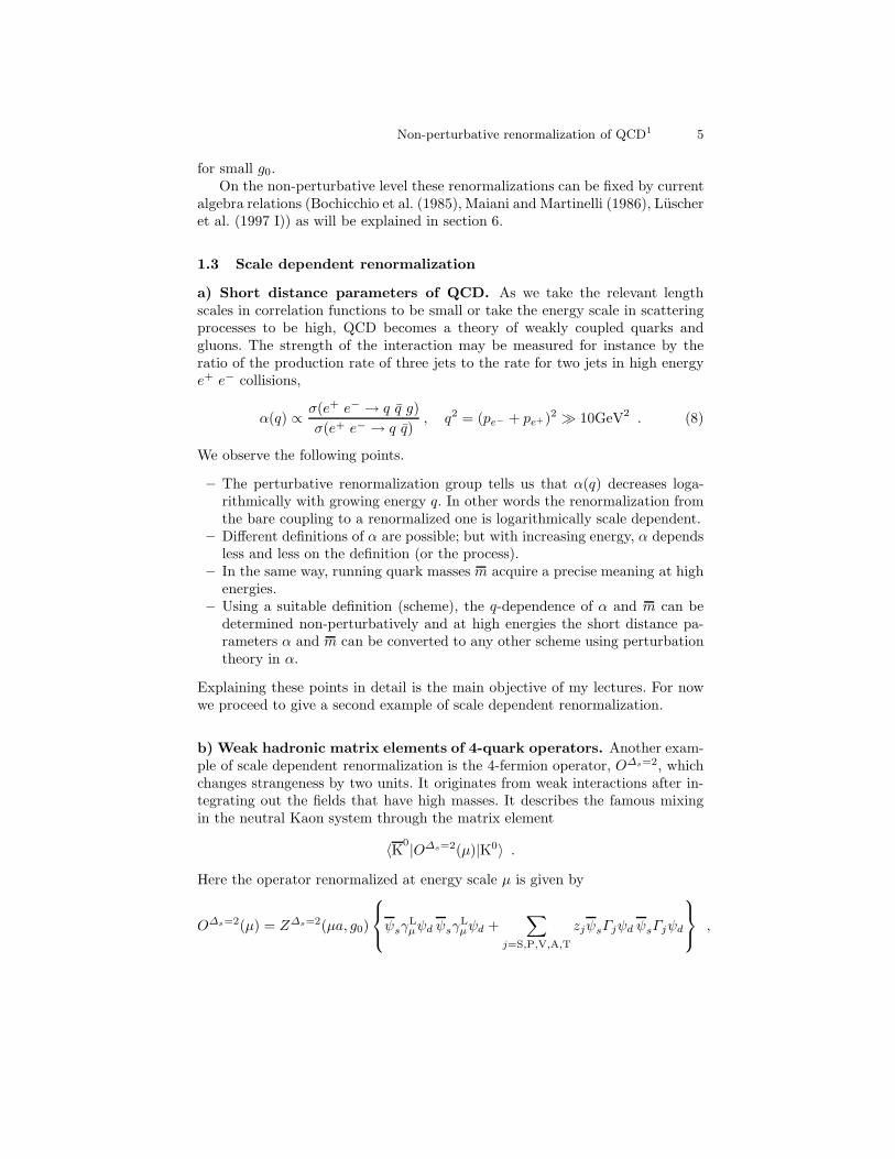
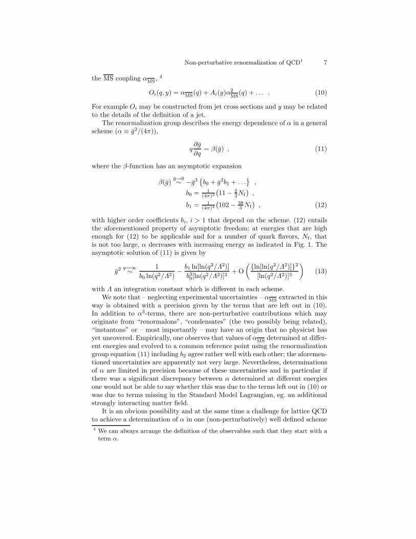
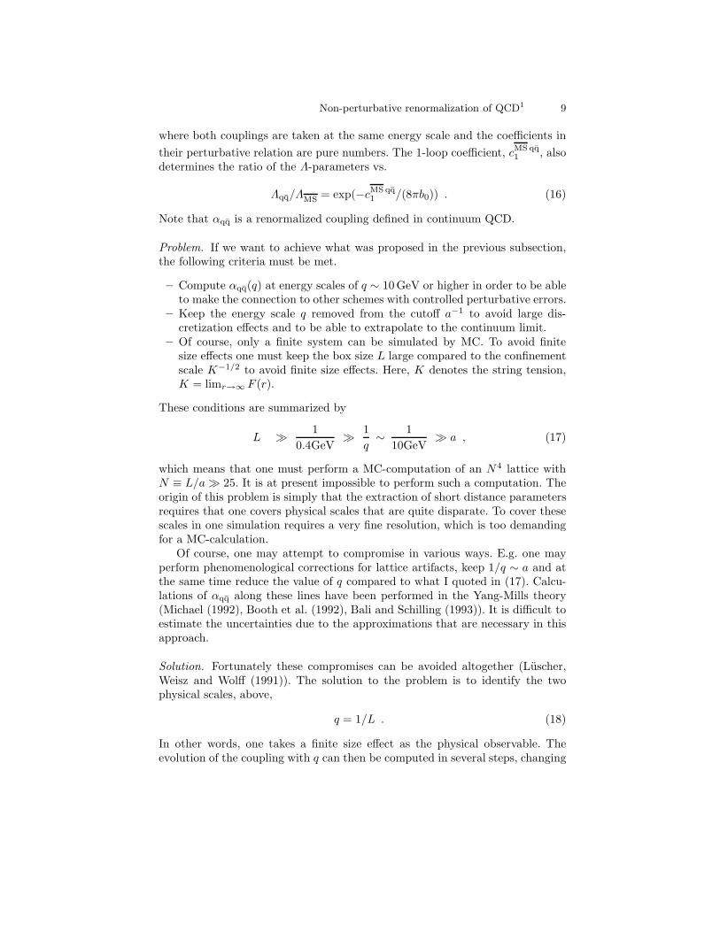
with higher order coefficients bi, i > 1 that depend on the scheme. (12) entailsthe aforementioned property of asymptotic freedom: at energies that are highenough for (12) to be applicable and for a number of quark flavors, Nf , thatis not too large, α decreases with increasing energy as indicated in Fig. 1. Theasymptotic solution of (11) is given by
g2 q→∞∼ 1
b0 ln(q2/Λ2)− b1 ln[ln(q2/Λ2)]
b30[ln(q2/Λ2)]2+ O
(ln[ln(q2/Λ2)]2
[ln(q2/Λ2)]3
)(13)
with Λ an integration constant which is different in each scheme.We note that – neglecting experimental uncertainties – αMS extracted in this
way is obtained with a precision given by the terms that are left out in (10).In addition to α3-terms, there are non-perturbative contributions which mayoriginate from “renormalons”, “condensates” (the two possibly being related),“instantons” or – most importantly – may have an origin that no physicist hasyet uncovered. Empirically, one observes that values of αMS determined at differ-ent energies and evolved to a common reference point using the renormalizationgroup equation (11) including b2 agree rather well with each other; the aforemen-tioned uncertainties are apparently not very large. Nevertheless, determinationsof α are limited in precision because of these uncertainties and in particular ifthere was a significant discrepancy between α determined at different energiesone would not be able to say whether this was due to the terms left out in (10) orwas due to terms missing in the Standard Model Lagrangian, eg. an additionalstrongly interacting matter field.
It is an obvious possibility and at the same time a challenge for lattice QCDto achieve a determination of α in one (non-perturbatively) well defined scheme
4 We can always arrange the definition of the observables such that they start with aterm α.
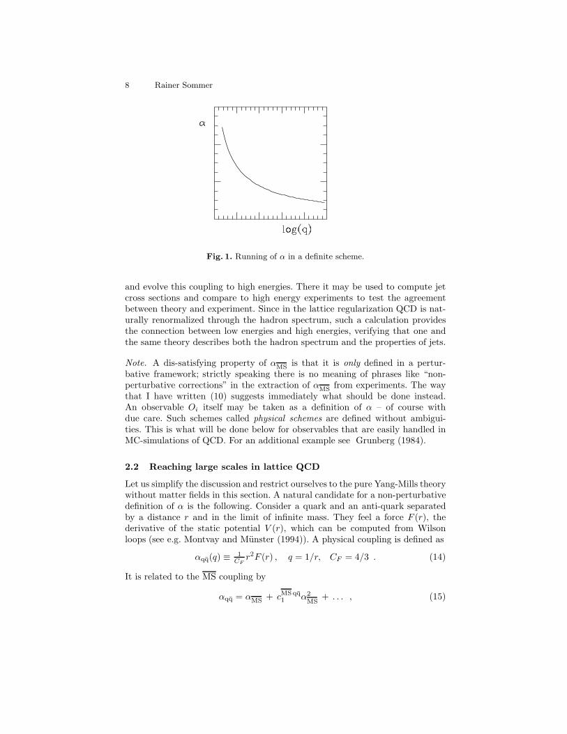
8 Rainer Sommer
Fig. 1. Running of α in a definite scheme.
and evolve this coupling to high energies. There it may be used to compute jetcross sections and compare to high energy experiments to test the agreementbetween theory and experiment. Since in the lattice regularization QCD is nat-urally renormalized through the hadron spectrum, such a calculation providesthe connection between low energies and high energies, verifying that one andthe same theory describes both the hadron spectrum and the properties of jets.
Note. A dis-satisfying property of αMS is that it is only defined in a pertur-bative framework; strictly speaking there is no meaning of phrases like “non-perturbative corrections” in the extraction of αMS from experiments. The waythat I have written (10) suggests immediately what should be done instead.An observable Oi itself may be taken as a definition of α – of course withdue care. Such schemes called physical schemes are defined without ambigui-ties. This is what will be done below for observables that are easily handled inMC-simulations of QCD. For an additional example see Grunberg (1984).
2.2 Reaching large scales in lattice QCD
Let us simplify the discussion and restrict ourselves to the pure Yang-Mills theorywithout matter fields in this section. A natural candidate for a non-perturbativedefinition of α is the following. Consider a quark and an anti-quark separatedby a distance r and in the limit of infinite mass. They feel a force F (r), thederivative of the static potential V (r), which can be computed from Wilsonloops (see e.g. Montvay and Munster (1994)). A physical coupling is defined as
αqq(q) ≡ 1CF
r2F (r) , q = 1/r, CF = 4/3 . (14)
It is related to the MS coupling by
αqq = αMS + cMSqq1 α2
MS+ . . . , (15)
Non-perturbative renormalization of QCD1 9
where both couplings are taken at the same energy scale and the coefficients in
their perturbative relation are pure numbers. The 1-loop coefficient, cMS qq1 , also
determines the ratio of the Λ-parameters vs.
Λqq/ΛMS = exp(−cMS qq1 /(8πb0)) . (16)
Note that αqq is a renormalized coupling defined in continuum QCD.
Problem. If we want to achieve what was proposed in the previous subsection,the following criteria must be met.
– Compute αqq(q) at energy scales of q ∼ 10 GeV or higher in order to be ableto make the connection to other schemes with controlled perturbative errors.
– Keep the energy scale q removed from the cutoff a−1 to avoid large dis-cretization effects and to be able to extrapolate to the continuum limit.
– Of course, only a finite system can be simulated by MC. To avoid finitesize effects one must keep the box size L large compared to the confinementscale K−1/2 to avoid finite size effects. Here, K denotes the string tension,K = limr→∞ F (r).
These conditions are summarized by
L ≫ 1
0.4GeV≫ 1
q∼ 1
10GeV≫ a , (17)
which means that one must perform a MC-computation of an N4 lattice withN ≡ L/a≫ 25. It is at present impossible to perform such a computation. Theorigin of this problem is simply that the extraction of short distance parametersrequires that one covers physical scales that are quite disparate. To cover thesescales in one simulation requires a very fine resolution, which is too demandingfor a MC-calculation.
Of course, one may attempt to compromise in various ways. E.g. one mayperform phenomenological corrections for lattice artifacts, keep 1/q ∼ a and atthe same time reduce the value of q compared to what I quoted in (17). Calcu-lations of αqq along these lines have been performed in the Yang-Mills theory(Michael (1992), Booth et al. (1992), Bali and Schilling (1993)). It is difficult toestimate the uncertainties due to the approximations that are necessary in thisapproach.
Solution. Fortunately these compromises can be avoided altogether (Luscher,Weisz and Wolff (1991)). The solution to the problem is to identify the twophysical scales, above,
q = 1/L . (18)
In other words, one takes a finite size effect as the physical observable. Theevolution of the coupling with q can then be computed in several steps, changing
10 Rainer Sommer
q by factors of order 2 in each step. In this way, no large scale ratios appear anddiscretization errors are small for L/a≫ 1.
For illustration, we modify the definition of αqq(q) to fit into this class offinite volume couplings. Consider the Yang-Mills theory on a T × L3 – toruswith T ≫ L.5 The finite volume coupling,
αqq(q) ≡ kr2F (r, L)r=L/4 , q = 1/L , (19)
can again be related to the MS coupling perturbatively,
αqq = αMS + cMSqq1 α2
MS+ . . . . (20)
This relation may come as a surprise since it relates a small volume quantityto an infinite volume one. Remember, however, that once the bare coupling andmasses are eliminated there are no free parameters. Renormalized couplings infinite volume and couplings in infinite volume are in one-to-one correspondence.When they are small they can be related by perturbation theory. In particular,(16) holds with the obvious modification.
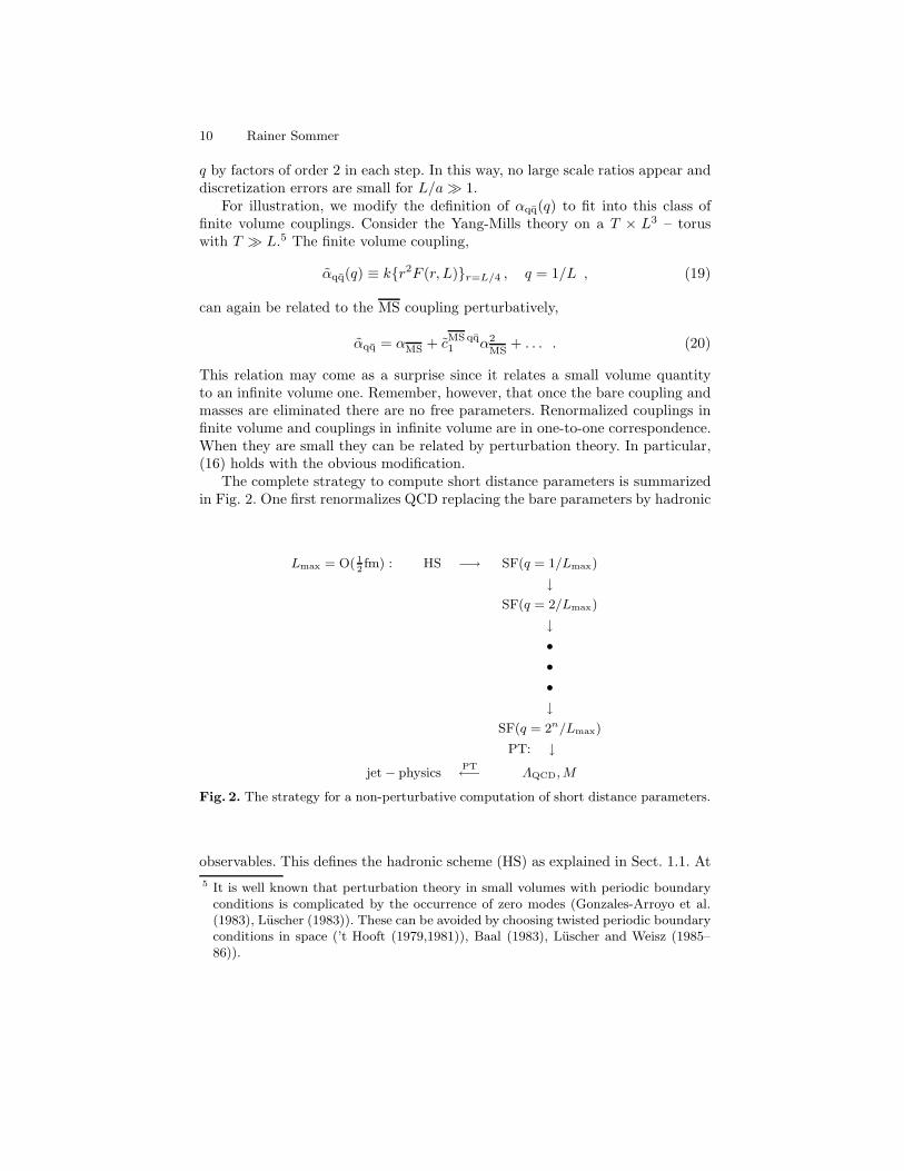
The complete strategy to compute short distance parameters is summarizedin Fig. 2. One first renormalizes QCD replacing the bare parameters by hadronic
Lmax = O( 12fm) : HS −→ SF(q = 1/Lmax)
↓
SF(q = 2/Lmax)
↓
•
•
•
↓
SF(q = 2n/Lmax)
PT: ↓
jet − physicsPT←− ΛQCD, M
Fig. 2. The strategy for a non-perturbative computation of short distance parameters.
observables. This defines the hadronic scheme (HS) as explained in Sect. 1.1. At
5 It is well known that perturbation theory in small volumes with periodic boundaryconditions is complicated by the occurrence of zero modes (Gonzales-Arroyo et al.(1983), Luscher (1983)). These can be avoided by choosing twisted periodic boundaryconditions in space (’t Hooft (1979,1981)), Baal (1983), Luscher and Weisz (1985–86)).
Non-perturbative renormalization of QCD1 11
a low energy scale q = 1/Lmax this scheme can be related to the finite volumescheme denoted by SF in the graph. Within this scheme one then computes thescale evolution up to a desired energy q = 2n/Lmax. As we will see it is noproblem to choose the number of steps n large enough to be sure that one isin the perturbative regime. There perturbation theory (PT) is used to evolvefurther to infinite energy and compute the Λ-parameter and the renormalizationgroup invariant quark masses. Inserted into perturbative expressions these pro-vide predictions for jet cross sections or other high energy observables. In thegraph all arrows correspond to relations in the continuum; the whole strategy isdesigned such that lattice calculations for these relations can be extrapolated tothe continuum limit.
For the practical success of the approach, the finite volume coupling (as wellas the corresponding quark mass) must satisfy a number of criteria.
– They should have an easy perturbative expansion, such that the β-function(and τ -function, which describes the evolution of the running masses) canbe computed to sufficient order.
– They should be easy to calculate in MC (small variance!).– Discretization errors must be small to allow for safe extrapolations to the
continuum limit.
Careful consideration of the above points led to the introduction of renormal-ized coupling and quark mass through the Schrodinger functional (SF) of QCD(Luscher et al. (1992), Luscher et al. (1993-94), Sint (1994-95), Jansen et al.(1996)). We introduce the SF in the following section. In the Yang-Mills the-ory, an alternative finite volume coupling was introduced in G. de Divitiis et al.(1994) and studied in detail in G. de Divitiis et al. (1995 I), G. de Divitiis et al.(1995 II) .
The criteria (17) apply quite generally to any scale dependent renormaliza-tion, e.g. the one described in Sect. 1.3 b. Although the details of the finite sizetechnique have not yet been developed for these cases, the same strategy can beapplied. This will certainly be the subject of future research. So far, the approachhas been to search for a “window” where q is high enough to apply PT but nottoo close to a−1 (Martinelli et al. (1994)). An essential advantage of the detailsof the approach of Martinelli et al. (1994) as applied to the renormalizationof composite quark operators is its simplicity: formulating the renormalizationconditions in a MOM-scheme, one may use results from perturbation theory ininfinite volume in the perturbative part of the matching. Since, however, highenergies q can not be reached in this approach, we will not discuss it further andrefer to Donini et al. (1995), Oelrich et al. (1997) for an account of the presentstatus and further references, instead. In particular, in the latter reference itcan be seen, how non-trivial it is to have a “window” where both perturbationtheory can be applied and lattice artifacts are small.
Note. (17) has been written for the Yang-Mills theory. In full QCD, finite sizeeffects will be more important and one should replace
√K → mπ, resulting in a
12 Rainer Sommer
more stringent requirement.
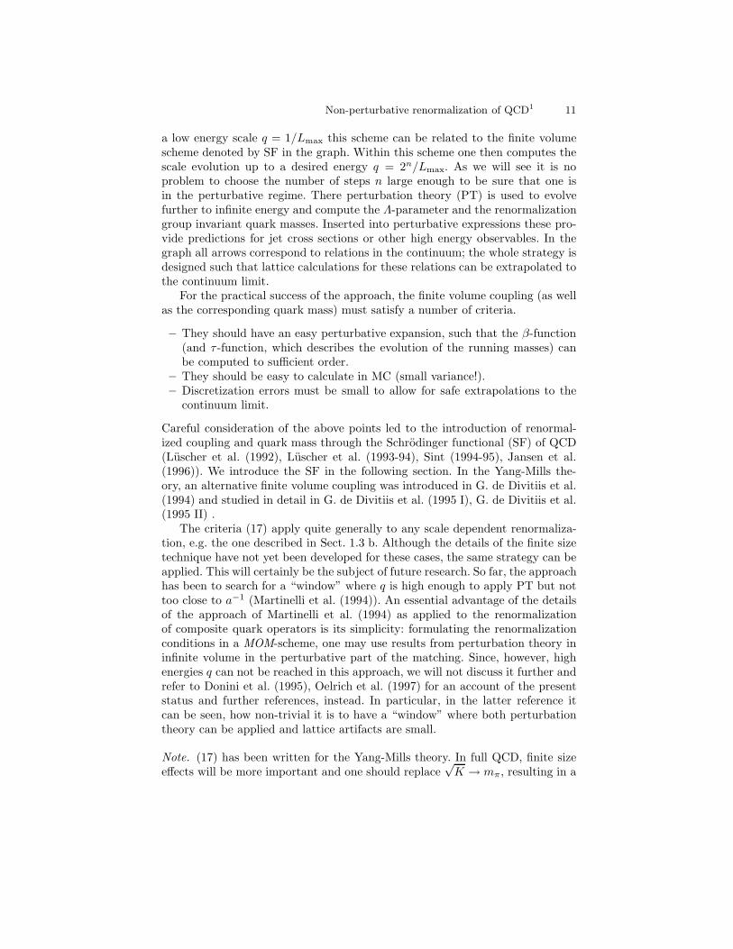
3 The Schrodinger functional
We want to introduce a specific finite volume scheme that fulfills all the require-ments explained in the previous section. It is defined from the SF of QCD, whichwe introduce below. For simplicity we restrict the discussion to the pure gaugetheory except for Sect. 3.7 and Sect. 3.8. Apart from the latter subsections, thepresentation follows closely Luscher et al. (1992); we refer to this work for furtherdetails as well as proofs of the properties described below.
space
(LxLxL box with periodic b.c.)
time
0
L
C’
C
Fig. 3. Illustration of the Schrodinger functional.
3.1 Definition
Here, we give a formal definition of the SF in the Yang-Mills theory in continuumspace-time, noting that a rigorous treatment is possible in the lattice regularizedtheory.
Space-time is taken to be a cylinder illustrated in Fig. 3. We impose Dirichletboundary conditions for the vector potentials6 in time,
Ak(x) =
CΛk (x) at x0 = 0C′
k(x) at x0 = L, (21)
where C, C′ are classical gauge potentials and AΛ denotes the gauge transformof A,
AΛk (x) = Λ(x)Ak(x)Λ(x)−1 + Λ(x)∂kΛ(x)−1, Λ ∈ SU(N) . (22)
6 We use anti-hermitian vector potentials. E.g. in the gauge group SU(2), we haveAµ(x) = Aa
µ(x)τa/(2i), in terms of the Pauli-matrices τa.
Non-perturbative renormalization of QCD1 13
In space, we impose periodic boundary conditions,
Ak(x+ Lk) = Ak(x), Λ(x + Lk) = Λ(x) . (23)
The (Euclidean) partition function with these boundary conditions defines theSF,
Z[C′, C] ≡∫
D[Λ]
∫D[A] e−SG[A] , (24)
SG[A] = − 1
2g20
∫d4x tr FµνFµν ,
Fµν = ∂µAν − ∂νAµ + [Aµ, Aν ] ,
D[A] =∏
x,µ,a
dAaµ(x), D[Λ] =∏
x
dΛ(x) .
Here dΛ(x) denotes the Haar measure of SU(N). It is easy to show that the SFis a gauge invariant functional of the boundary fields,
Z[C′Ω′
, CΩ] = Z[C′, C] , (25)
where also large gauge transformations are permitted. The invariance under thelatter is an automatic property of the SF defined on a lattice, while in thecontinuum formulation it is enforced by the integral over Λ in (24).
3.2 Quantum mechanical interpretation
The SF is the quantum mechanical transition amplitude from a state |C〉 to astate |C′〉 after a (Euclidean) time L. To explain the meaning of this statementof the SF, we introduce the Schrodinger representation. The Hilbert space con-sists of wave-functionals Ψ [A] which are functionals of the spatial components ofthe vector potentials, Aak(x). The canonically conjugate field variables are repre-sented by functional derivatives, Eak (x) = 1
iδ
δAa
k(x) , and a scalar product is given
by
〈Ψ |Ψ ′〉 =
∫D[A]Ψ [A]∗Ψ ′[A], D[A] =
∏
x,k,a
dAak(x) . (26)
The Hamilton operator,
IH =
∫ L
0
d3x
g20
2Eak (x)Eak (x) +
1
4g20
F akl(x)F akl(x)
, (27)
commutes with the projector, IP, onto the physical subspace of the Hilbert space(i.e. the space of gauge invariant states), where IP acts as
IPψ[A] =
∫D[Λ]ψ[AΛ] . (28)
14 Rainer Sommer
Finally, each classical gauge field defines a state |C〉 through
〈C|Ψ〉 = Ψ [C] . (29)
After these definitions, the quantum mechanical representation of the SF is givenby
Z[C′, C] = 〈C′|e−IHT IP|C〉
=∞∑
n=0
e−EnTΨn[C′]Ψn[C]∗ . (30)
In the lattice formulation, (30) can be derived rigorously and is valid with realenergy eigenvalues En.
3.3 Background field
A complementary aspect of the SF is that it allows a treatment of QCD in a colorbackground field in an unambiguous way. Let us assume that we have a solutionB of the equations of motion, which satisfies also the boundary conditions (21).If, in addition,
S[A] > S[B] (31)
for all gauge fields A that are not equal to a gauge transform BΩ of B, then wecall B the background field (induced by the boundary conditions). Here, Ω(x)is a gauge transformation defined for all x in the cylinder and its boundary andBΩ is the corresponding generalization of (22). Background fields B, satisfyingthese conditions are known; we will describe a particular family of fields, later.
Due to (31), fields close to B dominate the path integral for weak couplingg0 and the effective action,
Γ [B] ≡ − lnZ [C′, C] , (32)
has a regular perturbative expansion,
Γ [B] =1
g20
Γ0[B] + Γ1[B] + g20Γ2[B] + . . . , (33)
Γ0[B] ≡ g20S[B] .
Above we have used that due to our assumptions, the background field, B, andthe boundary values C,C′ are in one-to-one correspondence and have taken Bas the argument of Γ .
Non-perturbative renormalization of QCD1 15
3.4 Perturbative expansion
For the construction of the SF-scheme as a renormalization scheme, one needs tostudy the renormalization properties of the functional, Z. Luscher et al. (1992)have performed a one-loop calculation for arbitrary background field. The cal-culation is done in dimensional regularization with 3− 2ε space dimensions andone time dimension. One expands the field A in terms of the background fieldand a fluctuation field, q, as
Aµ(x) = Bµ(x) + g0qµ(x) . (34)
Then one adds a gauge fixing term (“background field gauge”) and the corre-sponding Fadeev-Popov term. Of course, care must be taken about the properboundary conditions in all these expressions. Integration over the quantum fieldand the ghost fields then gives
Γ1[B] = 12 ln det ∆1 − ln det ∆0 , (35)
where ∆1 is the fluctuation operator and ∆0 the Fadeev-Popov operator. Theresult can be cast in the form
Γ1[B] =ε→0
−b0εΓ0[B] + O(1) , (36)
with the important result that the only (for ε→ 0) singular term is proportionalto Γ0.
After renormalization of the coupling, i.e. the replacement of the bare cou-pling by gMS via
g20 = µ2εg2
MS(µ)[1 + z1(ε)g
2MS
(µ)], z1(ε) = −b0ε, (37)
the effective action is finite,
Γ [B]ε=0 =
1
g2MS
− b0[lnµ2 − 1
16π2
]Γ0[B]
− 12ζ
′(0|∆1) + ζ′(0|∆0) + O(g2MS
) (38)
ζ′(0|∆) =d
dsζ(s|∆)
∣∣∣∣s=0
, ζ(s|∆) = Tr∆−s .
Here, ζ′(0|∆) is a complicated functional of B, which is not known analyticallybut can be evaluated numerically for specific choices of B.
The important result of this calculation is that (apart from field independentterms that have been dropped everywhere) the SF is finite after eliminating g0in favor of gMS. The presence of the boundaries does not introduce any extradivergences. In the following subsection we argue that this property is correct ingeneral, not just in one-loop approximation.
16 Rainer Sommer
3.5 General renormalization properties
The relevant question here is whether local quantum field theories formulated onspace-time manifolds with boundaries develop divergences that are not present inthe absence of boundaries (periodic boundary conditions or infinite space-time).In general the answer is “yes, such additional divergences exist”. In particu-lar, Symanzik studied the φ4-theory with SF boundary conditions (Symanzik(1981)). In a proof valid to all orders of perturbation theory he was able to showthat the SF is finite after
– renormalization of the self-coupling, λ, and the mass, m,– and the addition of the boundary counter-terms
∫
x0=T
d3xZ1φ
2 + Z2φ∂0φ
+
∫
x0=0
d3xZ1φ
2 − Z2φ∂0φ. (39)
In other words, in addition to the standard renormalizations, one has to addcounter-terms formed by local composite fields integrated over the boundaries.One expects that in general, all fields with dimension d ≤ 3 have to be takeninto account. Already Symanzik conjectured that counter-terms with this prop-erty are sufficient to renormalize the SF of any quantum field theory in fourdimensions.
Since this conjecture forms the basis for many applications of the SF to thestudy of renormalization, we note a few points concerning its status.
– As mentioned, a proof to all orders of perturbation theory exists for the φ4
theory, only.– There is no gauge invariant local field with d ≤ 3 in the Yang–Mills theory.
Consequently no additional counter-term is necessary in accordance with the1-loop result described in the previous subsection.
– In the Yang–Mills theory it has been checked also by explicit 2–loop calcula-tions (Narayanan and Wolff (1995), Bode (1997)). Numerical, non-perturbative,MC simulations (Luscher et al. (1993-94), G. de Divitiis et al. (1995 II) ) givefurther support for its validity.
– It has been shown to be valid in QCD with quarks to 1-loop (Sint (1994-95)).– A straight forward application of power counting in momentum space in
order to prove the conjecture is not possible due to the missing translationinvariance.
Although a general proof is missing, there is little doubt that Symanzik’s con-jecture is valid in general. Concerning QCD, this puts us into the position togive an elegant definition of a renormalized coupling in finite volume.
3.6 Renormalized coupling
For the definition of a running coupling we need a quantity which depends onlyon one scale. We choose LB such that it depends only on one dimensionless vari-able η. In other words, the strength of the field is scaled as 1/L. The background
Non-perturbative renormalization of QCD1 17
field is assumed to fulfill the requirements of Sect. 3.3. Then, following the abovediscussion, the derivative
Γ ′[B] =∂
∂ηΓ [B] , (40)
is finite when it is expressed in terms of a renormalized coupling like gMS but Γ ′
is defined non-perturbatively. From (33) we read off immediately that a properlynormalized coupling is given by
g2(L) = Γ ′
0[B]/Γ ′[B] . (41)
Since there is only one length scale L, it is evident that g defined in this wayruns with L.
A specific choice for the gauge group SU(3) is the abelian background fieldinduced by the boundary values (Luscher et al. (1993-94))
Ck = iL
φ1 0 00 φ2 00 0 φ3
, C′
k = iL
φ′1 0 00 φ′2 00 0 φ′3
, k = 1, 2, 3, (42)
with
φ1 = η − π3 , φ′1 = −φ1 − 4π
3 ,
φ2 = − 12η, φ′2 = −φ3 + 2π
3 ,
φ3 = − 12η + π
3 , φ′3 = −φ2 + 2π3 .
(43)
In this case, the derivatives with respect to η are to be evaluated at η = 0. Theassociated background field,
B0 = 0, Bk = [x0C′
k + (L− x0)Ck] /L, k = 1, 2, 3 , (44)
has a field tensor with non-vanishing components
G0k = ∂0Bk = (C′
k − Ck)/L, k = 1, 2, 3 . (45)
It is a constant color-electric field.
3.7 Quarks
In the end, the real interest is in the renormalization of QCD and we need toconsider the SF with quarks. It has been discussed in Sint (1994-95).
Special care has to be taken in formulating the Dirichlet boundary conditionsfor the quark fields; since the Dirac operator is a first order differential operator,the Dirac equation has a unique solution when one half of the components of thefermion fields are specified on the boundaries. Indeed, a detailed investigationshows that the boundary condition
P+ψ|x0=0 = ρ, P−ψ|x0=L = ρ′ , P± = 12 (1 ± γ0) , (46)
ψP−|x0=0 = ρ, ψP+|x0=L = ρ′ , (47)
18 Rainer Sommer
lead to a quantum mechanical interpretation analogous to (30). The SF
Z[C′, ρ ′, ρ ′;C, ρ, ρ] =
∫D[A]D[ψ ]D[ψ ] e−S[A,ψ,ψ ] (48)
involves an integration over all fields with the specified boundary values. Thefull action may be written as
S[A,ψ, ψ ] = SG[ψ, ψ ] + SF[A,ψ, ψ ]
SF =
∫d4xψ(x)[γµDµ +m]ψ(x) (49)
−∫
d3x [ψ(x)P−ψ(x)]x0=0 −∫
d3x [ψ(x)P+ψ(x)]x0=L ,
with SG as given in (24). In (49) we use standard Euclidean γ-matrices. Thecovariant derivative, Dµ, acts as Dµψ(x) = ∂µψ(x) +Aµ(x)ψ(x).
Let us now discuss the renormalization of the SF with quarks. In contrast tothe pure Yang-Mills theory, gauge invariant composite fields of dimension threeare present in QCD. Taking into account the boundary conditions one finds (Sint(1994-95)) that the counter-terms,
ψP−ψ|x0=0 and ψP+ψ|x0=L , (50)
have to be added to the action with weight 1−Zb to obtain a finite renormalizedfunctional. These counter-terms are equivalent to a multiplicative renormaliza-tion of the boundary values,
ρR = Z−1/2b ρ , . . . , ρ′R = Z
−1/2b ρ′ . (51)
It follows that – apart from the renormalization of the coupling and the quarkmass – no additional renormalization of the SF is necessary for vanishing bound-ary values ρ, . . . , ρ′. So, after imposing homogeneous boundary conditions for thefermion fields, a renormalized coupling may be defined as in the previous sub-section.
As an important aside, we point out that the boundary conditions for thefermions introduce a gap into the spectrum of the Dirac operator (at least forweak couplings). One may hence simulate the lattice SF for vanishing phys-ical quark masses. It is then convenient to supplement the definition of therenormalized coupling by the requirement m = 0. In this way, one defines amass-independent renormalization scheme with simple renormalization groupequations. In particular, the β-function remains independent of the quark mass.
Correlation functions are given in terms of the expectation values of anyproduct O of fields,
〈O〉 =
1
Z
∫D[A]D[ψ ]D[ψ ]O e−S[A,ψ,ψ ]
ρ ′=ρ ′=ρ=ρ=0
, (52)
Non-perturbative renormalization of QCD1 19
evaluated for vanishing boundary values ρ, . . . , ρ′. Apart from the gauge field andthe quark and anti-quark fields integrated over, O may involve the “boundaryfields” (Luscher et al. (1996))
ζ(x) =δ
δρ(x), ζ(x) = − δ
δρ(x),
ζ′(x) =δ
δρ ′(x), ζ ′(x) = − δ
δρ ′(x). (53)
An application of fermionic correlation functions including the boundary fields isthe definition of the renormalized quark mass in the SF scheme to be discussednext.
3.8 Renormalized mass
Just as in the case of the coupling constant, there is a great freedom in defin-ing renormalized quark masses. A natural starting point is the PCAC relationwhich expresses the divergence of the axial current (5) in terms of the associatedpseudo-scalar density,
P a(x) = ψ(x)γ512τ
aψ(x) , (54)
via
∂µAaµ(x) = 2mP a(x) . (55)
This operator identity is easily derived at the classical level (cf. Sect. 6). Afterrenormalizing the operators,
(AR)aµ = ZAAaµ ,
P aR = ZPPa , (56)
a renormalized current quark mass may be defined by
m =ZA
ZPm . (57)
Here, m, is to be taken from (55) inserted into an arbitrary correlation functionand ZA can be determined unambiguously as mentioned in Sect. 1.2. Note thatmdoes not depend on which correlation function is used because the PCAC relationis an operator identity. The definition of m is completed by supplementing (56)with a specific normalization condition for the pseudo-scalar density. m theninherits its scheme- and scale-dependence from the corresponding dependenceof PR. Such a normalization condition may be imposed through infinite volumecorrelation functions. Since we want to be able to compute the running massfor large energy scales, we do, however, need a finite volume definition. This isreadily given in terms of correlation functions in the SF.
20 Rainer Sommer
space
time
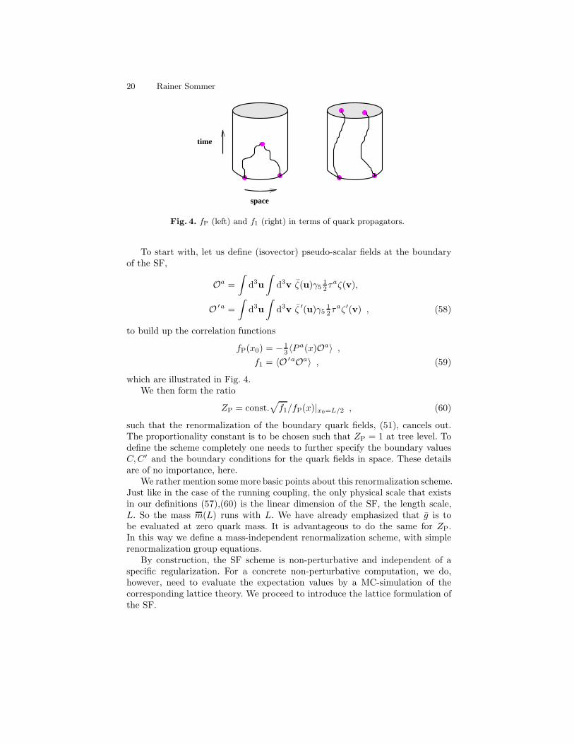
Fig. 4. fP (left) and f1 (right) in terms of quark propagators.
To start with, let us define (isovector) pseudo-scalar fields at the boundaryof the SF,
Oa =
∫d3u
∫d3v ζ(u)γ5
12τ
aζ(v),
O ′a =
∫d3u
∫d3v ζ ′(u)γ5
12τ
aζ′(v) , (58)
to build up the correlation functions
fP(x0) = − 13 〈P
a(x)Oa〉 ,f1 = 〈O ′aOa〉 , (59)
which are illustrated in Fig. 4.We then form the ratio
ZP = const.√f1/fP(x)|x0=L/2 , (60)
such that the renormalization of the boundary quark fields, (51), cancels out.The proportionality constant is to be chosen such that ZP = 1 at tree level. Todefine the scheme completely one needs to further specify the boundary valuesC,C′ and the boundary conditions for the quark fields in space. These detailsare of no importance, here.
We rather mention some more basic points about this renormalization scheme.Just like in the case of the running coupling, the only physical scale that existsin our definitions (57),(60) is the linear dimension of the SF, the length scale,L. So the mass m(L) runs with L. We have already emphasized that g is tobe evaluated at zero quark mass. It is advantageous to do the same for ZP.In this way we define a mass-independent renormalization scheme, with simplerenormalization group equations.
By construction, the SF scheme is non-perturbative and independent of aspecific regularization. For a concrete non-perturbative computation, we do,however, need to evaluate the expectation values by a MC-simulation of thecorresponding lattice theory. We proceed to introduce the lattice formulation ofthe SF.
Non-perturbative renormalization of QCD1 21
3.9 Lattice formulation
A detailed knowledge of the form of the lattice action is not required for anunderstanding of the following sections. Nevertheless, we give a definition of theSF in lattice regularization. This is done both for completeness and because itallows us to obtain a first impression about the size of discretization errors.
We choose a hyper-cubic Euclidean lattice with spacing a. A gauge field U onthe lattice is an assignment of a matrix U(x, µ) ∈ SU(N) to every lattice pointx and direction µ = 0, 1, 2, 3. Quark and anti-quark fields, ψ(x) and ψ(x), resideon the lattice sites and carry Dirac, color and flavor indices as in the continuum.To be able to write the quark action in an elegant form it is useful to extend thefields, initially defined only inside the SF manifold (cf. Fig. 3) to all times x0 by“padding” with zeros. In the case of the quark field one sets
ψ(x) = 0 if x0 < 0 or x0 > L,
andP−ψ(x)|x0=0 = P+ψ(x)|x0=L = 0,
and similarly for the anti-quark field. Gauge field variables that reside outsidethe manifold are set to 1.
We may then write the fermionic action as a sum over all space-time pointswithout restrictions for the time-coordinate,
SF[U, ψ, ψ] = a4∑
x
ψ(D +m0)ψ, (61)
and with the standard Wilson-Dirac operator,
D = 12
3∑
µ=0
γµ(∇∗
µ + ∇µ) − a∇∗
µ∇µ . (62)
Here, forward and backward covariant derivatives,
∇µψ(x) = 1a [U(x, µ)ψ(x + aµ) − ψ(x)], (63)
∇∗
µψ(x) = 1a [ψ(x) − U(x− aµ, µ)−1ψ(x− aµ)] , (64)
are used and m0 is to be understood as a diagonal matrix in flavor space withelements mf
0 .The gauge field action SG is a sum over all oriented plaquettes p on the
lattice, with the weight factors w(p), and the parallel transporters U(p) aroundp,
SG[U ] =1
g20
∑
p
w(p) tr 1 − U(p) . (65)
The weights w(p) are 1 for plaquettes in the interior and
w(p) =
12cs if p is a spatial plaquette at x0 = 0 or x0 = L,ct if p is time-like and attached to a boundary plane.
(66)
22 Rainer Sommer
The choice cs = ct = 1 corresponds to the standard Wilson action. However,these parameters can be tuned in order to reduce lattice artifacts, as will bebriefly discussed below.
With these ingredients, the path integral representation of the Schrodingerfunctional reads (Sint (1994-95)),
Z =
∫D[ψ]D[ψ ]D[U ] e−S , S = SF + SG , (67)
D[U ] =∏
x,µ
dU(x, µ) ,
with the Haar measure dU .
Boundary conditions and the background field. The boundary conditionsfor the lattice gauge fields may be obtained from the continuum boundary valuesby forming the appropriate parallel transporters from x+ ak to x at x0 = 0 andx0 = L. For the constant abelian boundary fields C and C′ that we consideredbefore, they are simply
U(x, k)|x0=0 = exp(aCk), U(x, k)|x0=L = exp(aC′
k), (68)
for k = 1, 2, 3. All other boundary conditions are as in the continuum.For the case of (42),(43), the boundary conditions (68) lead to a unique (up to
gauge transformations) minimal action configuration V , the lattice backgroundfield. It can be expressed in terms of B (44),
V (x, µ) = exp aBµ(x) . (69)
Lattice artifacts. Now we want to get a first impression about the dependenceof the lattice SF on the value of the lattice spacing. In other words we studylattice artifacts. At lowest order in the bare coupling we have, just like in thecontinuum,
Γ =1
g20
Γ0[V ] + O((g0)0) , Γ0[V ] ≡ g2
0SG[V ] . (70)
Furthermore one easily finds the action for small lattice spacings,
SG[V ] =[1 + (1 − ct)
2aL
] 3L4
g20
N∑
α=1
2
a2sin
[a2
2L2(φ′α − φα)
]2
=3
g20
N∑
α=1
(φ′α − φα)2 [
1 + (1 − ct)2aL + O(a4)
]. (71)
We observe: at tree-level of perturbation theory, all linear lattice artifacts areremoved when one sets ct = 1. Beyond tree-level, one has to tune the coefficientct as a function of the bare coupling. We will show the effect, when this is done to
Non-perturbative renormalization of QCD1 23
first order in g20 , below. Note that the existence of linear O(a) errors in the Yang-
Mills theory is special to the SF; they originate from dimension four operatorsF0kF0k and FklFkl which are irrelevant terms (i.e. they carry an explicit factorof the lattice spacing) when they are integrated over the surfaces. cs, which canbe tuned to cancel the effects of FklFkl, does not appear for the electric fieldthat we discussed above.
Once quark fields are present, there are more irrelevant operators that cangenerate O(a) effects as discussed in detail in Luscher et al. (1996). Here weemphasize a different feature of (71): once the O(a)-terms are canceled, theremaining a-effects are tiny. This special feature of the abelian background fieldis most welcome for the numerical computation of the running coupling; it allowsfor reliable extrapolations to the continuum limit.
Explicit expression for Γ ′. Let us finally explain that Γ ′ is an observablethat can easily be calculated in a MC simulation. From its definition we findimmediately
Γ ′ = − ∂
∂ηln
∫D[ψ]D[ψ ]D[U ] e−S
=
⟨∂S
∂η
⟩. (72)
The derivative ∂S∂η evaluates to the (color 8 component of the) electric field at
the boundary,
∂S
∂η= − 2
g20 L
a3∑
x
E8k(x) − (E8
k)′(x)
, (73)
E8k(x) =
1
a2Re tr
iλ8U(x, k)U(x + ak, 0)U(x+ a0, k)−1U(x, 0)−1
x0=0,
where λ8 = diag(1,−1/2,−1/2). (A similar expression holds for (E8k)
′(x)). Therenormalized coupling is therefore given in terms of the expectation value of alocal operator; no correlation function is involved. This means that it is easy andfast in computer time to evaluate it. It further turns out that a good statisticalprecision is reached with a moderate size statistical ensemble.
4 The computation of α(q)
We are now in the position to explain the details of Fig. 2 (Luscher, Weisz andWolff (1991), Luscher et al. (1993-94), Capitani et al. (1997)). The problem hasbeen solved in the SU(3) Yang-Mills theory. In the present context, this is ofcourse equivalent to the quenched approximation of QCD or the limit of zeroflavors. We will therefore also refer to results in quenched QCD.
Our central observable is the step scaling function that describes the scale-evolution of the coupling, i.e. moving vertically in Fig. 2. The analogous functionfor the running quark mass will be discussed in the following section.
24 Rainer Sommer
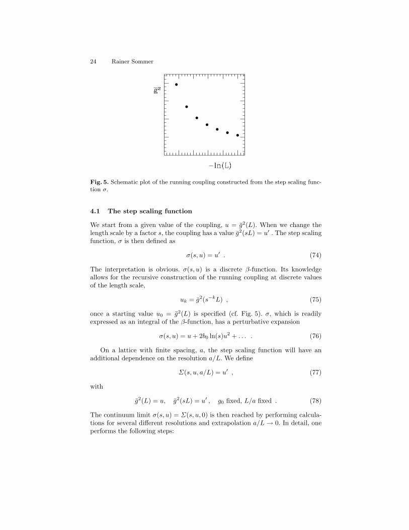
Fig. 5. Schematic plot of the running coupling constructed from the step scaling func-tion σ.
4.1 The step scaling function
We start from a given value of the coupling, u = g2(L). When we change thelength scale by a factor s, the coupling has a value g2(sL) = u′ . The step scalingfunction, σ is then defined as
σ(s, u) = u′ . (74)
The interpretation is obvious. σ(s, u) is a discrete β-function. Its knowledgeallows for the recursive construction of the running coupling at discrete valuesof the length scale,
uk = g2(s−kL) , (75)
once a starting value u0 = g2(L) is specified (cf. Fig. 5). σ, which is readilyexpressed as an integral of the β-function, has a perturbative expansion
σ(s, u) = u+ 2b0 ln(s)u2 + . . . . (76)
On a lattice with finite spacing, a, the step scaling function will have anadditional dependence on the resolution a/L. We define
Σ(s, u, a/L) = u′ , (77)
with
g2(L) = u, g2(sL) = u′ , g0 fixed, L/a fixed . (78)
The continuum limit σ(s, u) = Σ(s, u, 0) is then reached by performing calcula-tions for several different resolutions and extrapolation a/L → 0. In detail, oneperforms the following steps:
Non-perturbative renormalization of QCD1 25
1. Choose a lattice with L/a points in each direction.2. Tune the bare coupling g0 such that the renormalized coupling g2(L) has
the value u.3. At the same value of g0, simulate a lattice with twice the linear size; computeu′ = g2(2L). This determines the lattice step scaling function Σ(2, u, a/L).
4. Repeat steps 1.–3. with different resolutions L/a and extrapolate a/L→ 0.
Note that step 2. takes care of the renormalization and 3. determines the evolu-tion of the renormalized coupling.
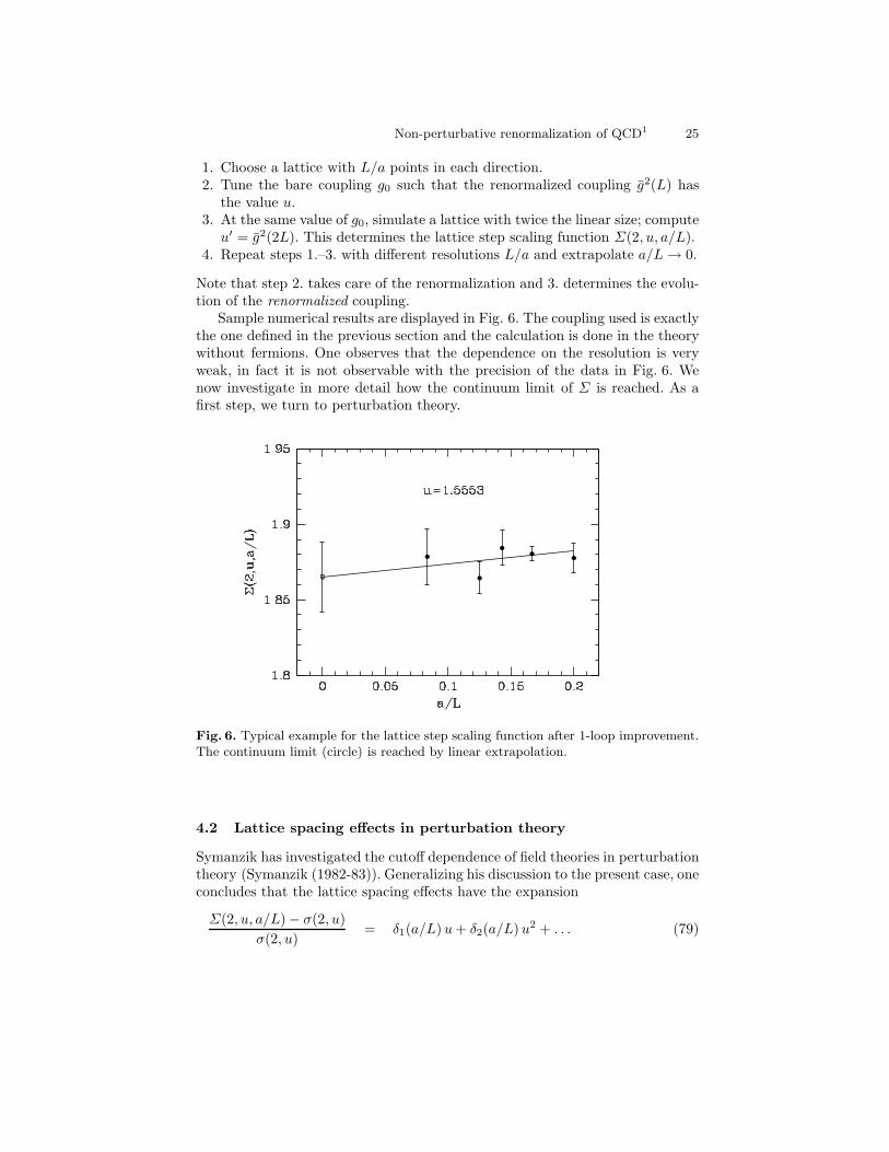
Sample numerical results are displayed in Fig. 6. The coupling used is exactlythe one defined in the previous section and the calculation is done in the theorywithout fermions. One observes that the dependence on the resolution is veryweak, in fact it is not observable with the precision of the data in Fig. 6. Wenow investigate in more detail how the continuum limit of Σ is reached. As afirst step, we turn to perturbation theory.
Fig. 6. Typical example for the lattice step scaling function after 1-loop improvement.The continuum limit (circle) is reached by linear extrapolation.
4.2 Lattice spacing effects in perturbation theory
Symanzik has investigated the cutoff dependence of field theories in perturbationtheory (Symanzik (1982-83)). Generalizing his discussion to the present case, oneconcludes that the lattice spacing effects have the expansion
Σ(2, u, a/L)− σ(2, u)
σ(2, u)= δ1(a/L)u+ δ2(a/L)u2 + . . . (79)
26 Rainer Sommer
δn(a/L)a/L→0∼
n∑
k=0
ek,n[ln( aL )]k(aL
)+ dk,n[ln( aL )]k
(aL
)2+ . . . .
We expect that the continuum limit is reached with corrections O(a/L) alsobeyond perturbation theory. In this context O(a/L) summarizes terms that con-tain at least one power of a/L and may be modified by logarithmic correctionsas it is the case in (79). To motivate this expectation recall Sect. 1.4, where weexplained that lattice artifacts correspond to irrelevant operators7, which carryexplicit factors of the lattice spacing. Of course, an additional a-dependencecomes from their anomalous dimension, but in an asymptotically free theorysuch as QCD, this just corresponds to a logarithmic (in a) modification.
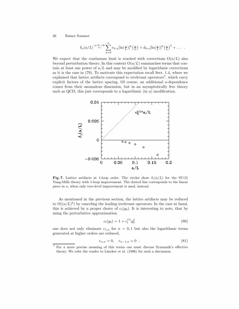
Fig. 7. Lattice artifacts at 1-loop order. The circles show δ1(a/L) for the SU(3)Yang-Mills theory with 1-loop improvement. The dotted line corresponds to the linearpiece in a, when only tree-level improvement is used, instead.
As mentioned in the previous section, the lattice artifacts may be reducedto O((a/L)2) by canceling the leading irrelevant operators. In the case at hand,this is achieved by a proper choice of ct(g0). It is interesting to note, that byusing the perturbative approximation
ct(g0) = 1 + c(1)t g2
0 (80)
one does not only eliminate e1,n for n = 0, 1 but also the logarithmic termsgenerated at higher orders are reduced,
en,n = 0, en−1,n = 0 . (81)7 For a more precise meaning of this terms one must discuss Symanzik’s effective
theory. We refer the reader to Luscher et al. (1996) for such a discussion.
Non-perturbative renormalization of QCD1 27
For tree-level improvement, ct(g0) = 1, the corresponding statement is en,n = 0.Heuristically, the latter is easy to understand. Tree-level improvement meansthat the propagators and vertices agree with the continuum ones up to correc-tions of order O(a2). Terms proportional to a can then arise only through alinear divergence of the Feynman diagrams. Once this happens, one cannot havethe maximum number of logarithmic divergences any more; consequently en,nvanishes.
To demonstrate further that the abelian field introduced in the previoussection induces small lattice artifacts, we show δ1(a/L) for the one loop improved
case. The term that is canceled by the proper choice c(1)t = −0.089 is shown as a
dashed line. The left over O((a/L)2)-terms are below the 1% level for couplingsu ≤ 2 and lattice sizes L/a ≥ 6. We now understand better why the a/L-dependence is so small in Fig. 6.
From the investigation of lattice spacing effects in perturbation theory oneexpects that one may safely extrapolate to the continuum limit by a fit
Σ(2, u, a/L) = σ(2, u) + const.× a/L , (82)
once one has data with a weak dependence on a/L, like the ones in Fig. 6. Suchan extrapolation is shown in the figure.
4.3 The continuum limit – universality
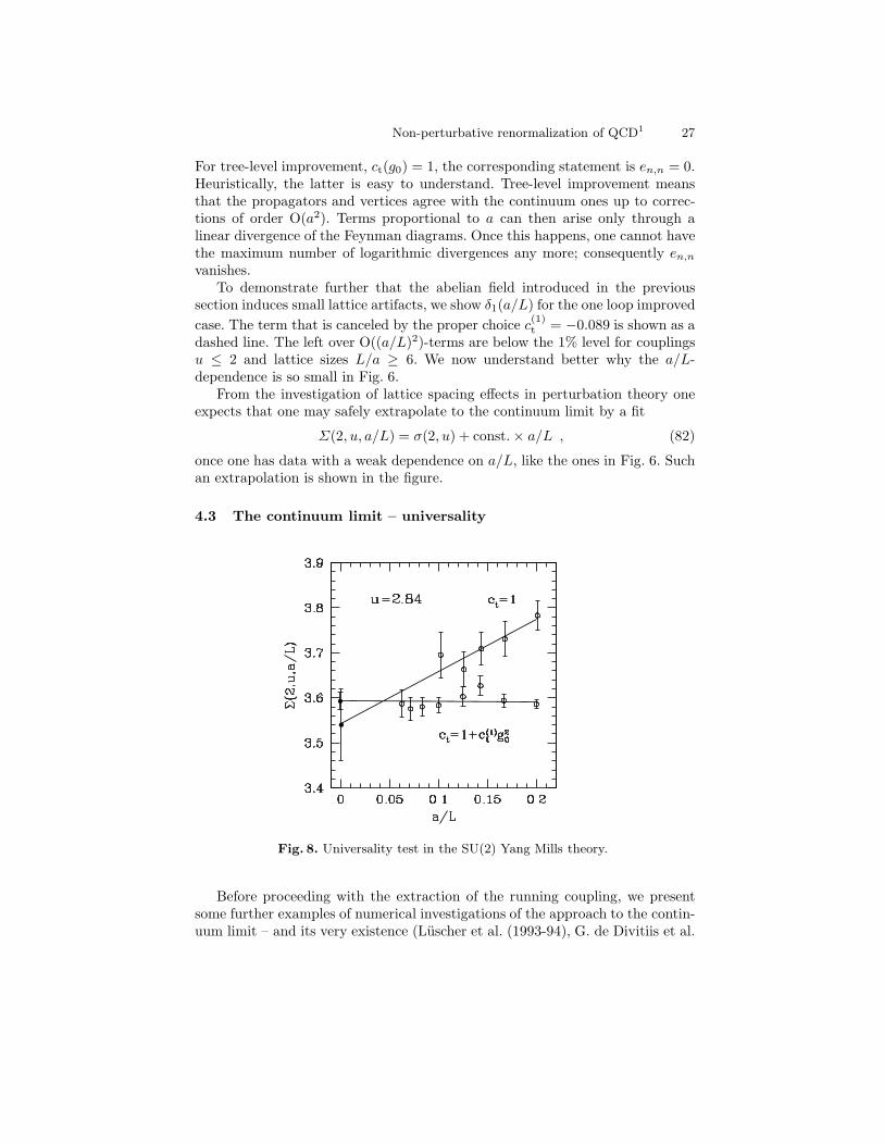
Fig. 8. Universality test in the SU(2) Yang Mills theory.
Before proceeding with the extraction of the running coupling, we presentsome further examples of numerical investigations of the approach to the contin-uum limit – and its very existence (Luscher et al. (1993-94), G. de Divitiis et al.
28 Rainer Sommer
(1995 II) ). The first example is the step scaling function in the SU(2) Yang-Millstheory (G. de Divitiis et al. (1995 II) ). Here we can compare the step scalingfunction obtained with two different lattice actions, one using tree-level O(a)improvement and the other one using ct at 1-loop order. (Fig. 8).
Not only does one observe a substantial reduction of the O(a)-errors throughperturbative improvement, but the very agreement of the two calculations whenextrapolated to a = 0, leaves little doubt that the continuum limit of the SFexists and is independent of the lattice action. In turn this also supports thestatement that the SF is renormalized after the renormalization of the couplingconstant.
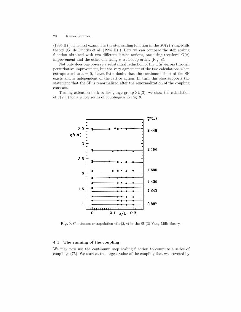
Turning attention back to the gauge group SU(3), we show the calculationof σ(2, u) for a whole series of couplings u in Fig. 9.
Fig. 9. Continuum extrapolation of σ(2, u) in the SU(3) Yang-Mills theory.
4.4 The running of the coupling
We may now use the continuum step scaling function to compute a series ofcouplings (75). We start at the largest value of the coupling that was covered by
Non-perturbative renormalization of QCD1 29
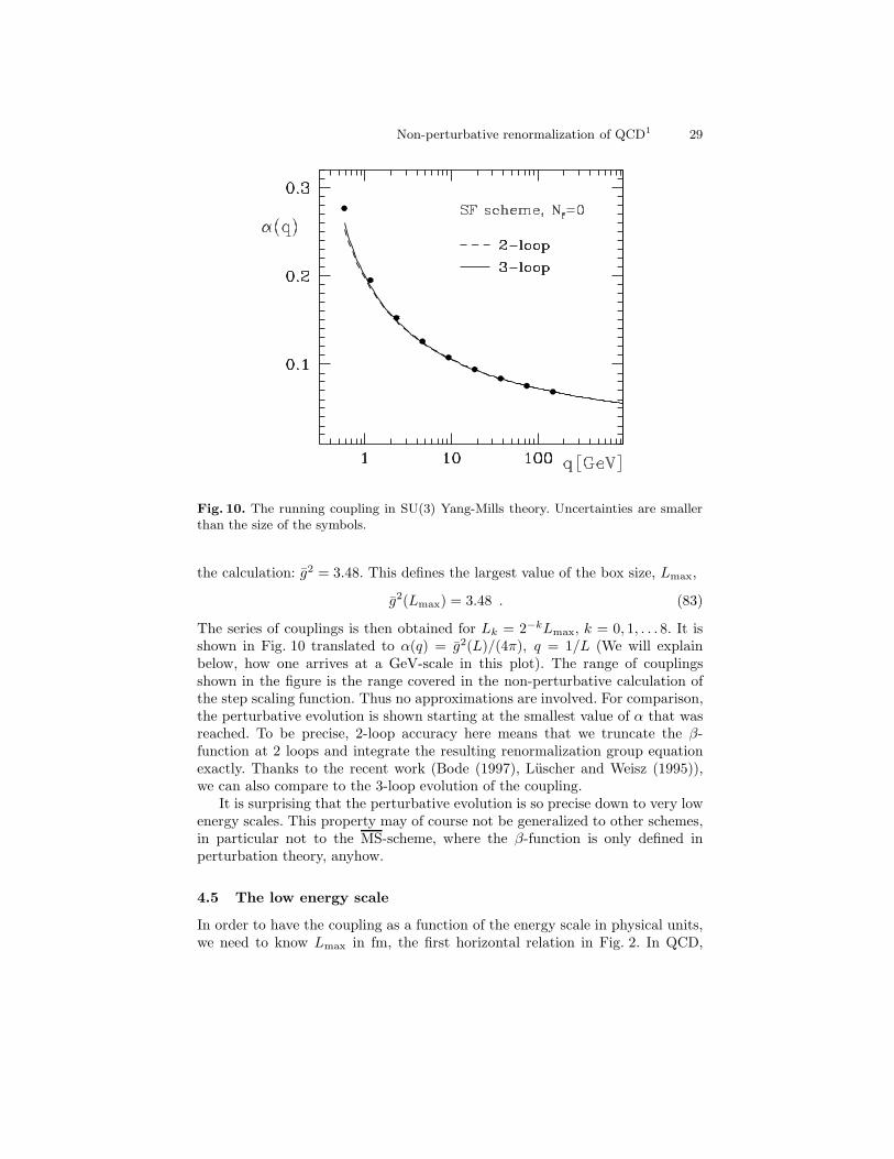
Fig. 10. The running coupling in SU(3) Yang-Mills theory. Uncertainties are smallerthan the size of the symbols.
the calculation: g2 = 3.48. This defines the largest value of the box size, Lmax,
g2(Lmax) = 3.48 . (83)
The series of couplings is then obtained for Lk = 2−kLmax, k = 0, 1, . . . 8. It isshown in Fig. 10 translated to α(q) = g2(L)/(4π), q = 1/L (We will explainbelow, how one arrives at a GeV-scale in this plot). The range of couplingsshown in the figure is the range covered in the non-perturbative calculation ofthe step scaling function. Thus no approximations are involved. For comparison,the perturbative evolution is shown starting at the smallest value of α that wasreached. To be precise, 2-loop accuracy here means that we truncate the β-function at 2 loops and integrate the resulting renormalization group equationexactly. Thanks to the recent work (Bode (1997), Luscher and Weisz (1995)),we can also compare to the 3-loop evolution of the coupling.
It is surprising that the perturbative evolution is so precise down to very lowenergy scales. This property may of course not be generalized to other schemes,in particular not to the MS-scheme, where the β-function is only defined inperturbation theory, anyhow.
4.5 The low energy scale
In order to have the coupling as a function of the energy scale in physical units,we need to know Lmax in fm, the first horizontal relation in Fig. 2. In QCD,
30 Rainer Sommer
this should be done by computing, for example, the product mpLmax with mp
the proton mass and then inserting the experimentally determined value of theproton mass.
At present, results like the ones shown in Fig. 10 are available for the Yang-Mills theory, only. Therefore, strictly speaking, there is no experimental observ-able to take over the role of the proton mass. As a purely theoretical exercise,one could replace the proton mass by a glueball mass; here, we choose a lengthscale, r0, derived from the force between static quarks, instead (Sommer(1994)).This quantity can be computed with better precision. Also one may argue thatthe static force is less influenced by whether one has dynamical quark loops inthe theory or not.
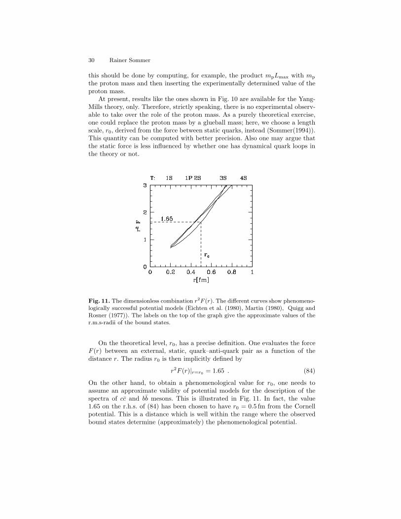
Fig. 11. The dimensionless combination r2F (r). The different curves show phenomeno-logically successful potential models (Eichten et al. (1980), Martin (1980), Quigg andRosner (1977)). The labels on the top of the graph give the approximate values of ther.m.s-radii of the bound states.
On the theoretical level, r0, has a precise definition. One evaluates the forceF (r) between an external, static, quark–anti-quark pair as a function of thedistance r. The radius r0 is then implicitly defined by
r2F (r)|r=r0 = 1.65 . (84)
On the other hand, to obtain a phenomenological value for r0, one needs toassume an approximate validity of potential models for the description of thespectra of cc and bb mesons. This is illustrated in Fig. 11. In fact, the value1.65 on the r.h.s. of (84) has been chosen to have r0 = 0.5 fm from the Cornellpotential. This is a distance which is well within the range where the observedbound states determine (approximately) the phenomenological potential.
Non-perturbative renormalization of QCD1 31
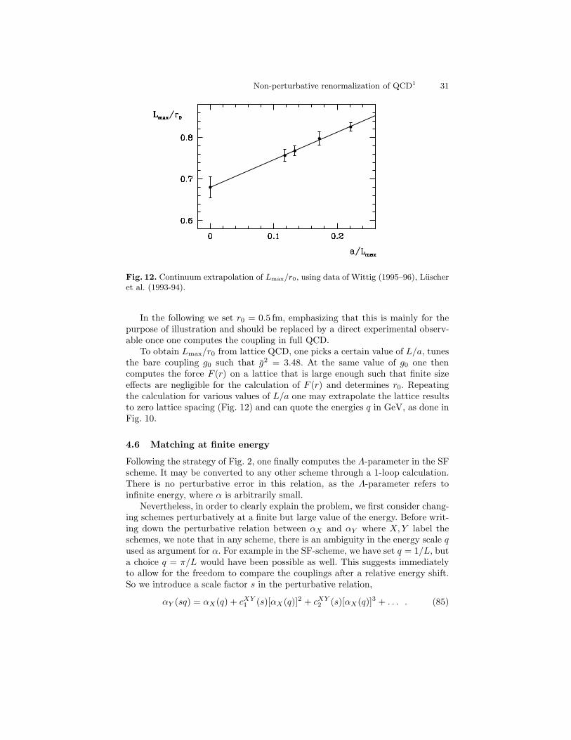
Fig. 12. Continuum extrapolation of Lmax/r0, using data of Wittig (1995–96), Luscheret al. (1993-94).
In the following we set r0 = 0.5 fm, emphasizing that this is mainly for thepurpose of illustration and should be replaced by a direct experimental observ-able once one computes the coupling in full QCD.
To obtain Lmax/r0 from lattice QCD, one picks a certain value of L/a, tunesthe bare coupling g0 such that g2 = 3.48. At the same value of g0 one thencomputes the force F (r) on a lattice that is large enough such that finite sizeeffects are negligible for the calculation of F (r) and determines r0. Repeatingthe calculation for various values of L/a one may extrapolate the lattice resultsto zero lattice spacing (Fig. 12) and can quote the energies q in GeV, as done inFig. 10.
4.6 Matching at finite energy
Following the strategy of Fig. 2, one finally computes the Λ-parameter in the SFscheme. It may be converted to any other scheme through a 1-loop calculation.There is no perturbative error in this relation, as the Λ-parameter refers toinfinite energy, where α is arbitrarily small.
Nevertheless, in order to clearly explain the problem, we first consider chang-ing schemes perturbatively at a finite but large value of the energy. Before writ-ing down the perturbative relation between αX and αY where X,Y label theschemes, we note that in any scheme, there is an ambiguity in the energy scale qused as argument for α. For example in the SF-scheme, we have set q = 1/L, buta choice q = π/L would have been possible as well. This suggests immediatelyto allow for the freedom to compare the couplings after a relative energy shift.So we introduce a scale factor s in the perturbative relation,
αY (sq) = αX(q) + cXY1 (s)[αX(q)]2 + cXY2 (s)[αX(q)]3 + . . . . (85)

32 Rainer Sommer
A natural and non-trivial question is now, which scale ratio s is optimal. Apossible criterion is to choose s such that the available terms in the perturbativeseries (85) are as small as possible. Since the number of available terms in theseries is usually low, we concentrate here on the possibility to set the first non-trivial term to zero. When available, the higher order one(s) may be used to testthe success of this procedure.
Scheme X cX MS1 (1) cX MS
2 (1) cX MS2 (s0)
qq −0.0821 −2.24 −2.19SF 1.256 2.775 0.27SF SU(2) 0.943 1.411 0.058TP SU(2) −0.558
Table 1. Examples for perturbative coefficients in (85) for Nf = 0.
So we fix s by requiring cXY1 (s) = 0 , which is satisfied for s = s0 with
s0 = exp−cXY1 (1)/(8πb0) = ΛX/ΛY , (86)
a relative shift given by the ratio of the Λ-parameters in the two schemes. Ex-amples taken from the literature (Luscher et al. (1992), Luscher et al. (1993-94), Narayanan and Wolff (1995), Bode (1997), Luscher and Weisz (1995), Fish-ler (1977), Sint and Sommer (1996), Billoire (1980), Peter (1997)) are listed inTable 1. In the case of matching the SF-scheme to MS, the use of s0 does in-deed reduce the 2-loop coefficient considerably. However for the qq-scheme s0 isclose to one and the 2-loop coefficient remains quite big. Not too surprisingly,no universal success of (86) is seen.
A non-perturbative test of the perturbative matching has been carried outby G. de Divitiis et al. (1995 II) in the SU(2) Yang-Mills theory, where the SF-scheme was related to a different finite volume scheme, called TP.8 The matchingcoefficient for this case is also listed in Table 1. Non-perturbatively the matchingwas computed as follows.
– For fixed L/a, the bare coupling was tuned such that g2SF(L) = 2.0778 (or
equivalently αSF(q = 1/L) = 0.1653).
– At the same bare coupling g2TP(L) was computed.
– These steps were repeated for a range of a/L and the results for g2TP(L) were
extrapolated to the continuum.
The result is shown in Fig. 13.
8 For the definition of the TP-scheme we refer the reader to the literature (G. deDivitiis et al. (1994), G. de Divitiis et al. (1995 I)).
Non-perturbative renormalization of QCD1 33
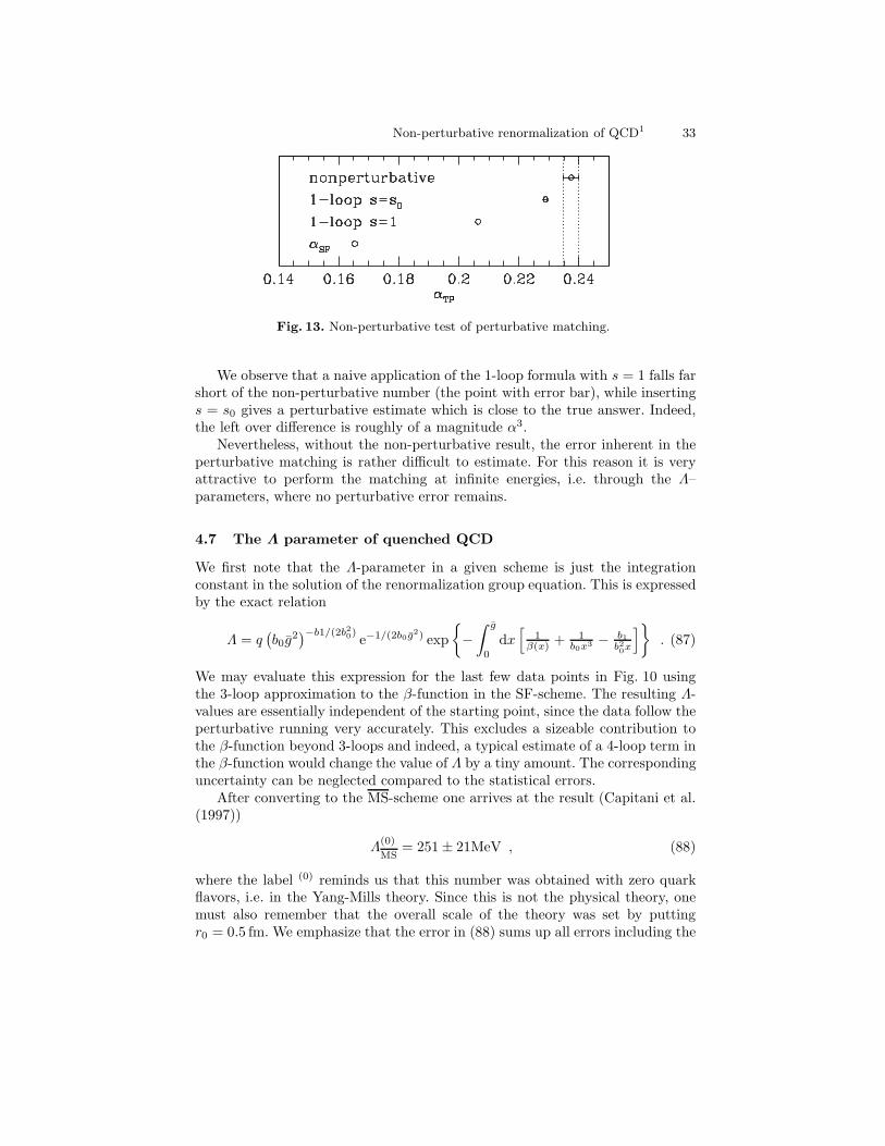
Fig. 13. Non-perturbative test of perturbative matching.
We observe that a naive application of the 1-loop formula with s = 1 falls farshort of the non-perturbative number (the point with error bar), while insertings = s0 gives a perturbative estimate which is close to the true answer. Indeed,the left over difference is roughly of a magnitude α3.
Nevertheless, without the non-perturbative result, the error inherent in theperturbative matching is rather difficult to estimate. For this reason it is veryattractive to perform the matching at infinite energies, i.e. through the Λ–parameters, where no perturbative error remains.
4.7 The Λ parameter of quenched QCD
We first note that the Λ-parameter in a given scheme is just the integrationconstant in the solution of the renormalization group equation. This is expressedby the exact relation
Λ = q(b0g
2)−b1/(2b20)
e−1/(2b0g2) exp
−
∫ g
0
dx[
1β(x) + 1
b0x3 − b1b20x
]. (87)
We may evaluate this expression for the last few data points in Fig. 10 usingthe 3-loop approximation to the β-function in the SF-scheme. The resulting Λ-values are essentially independent of the starting point, since the data follow theperturbative running very accurately. This excludes a sizeable contribution tothe β-function beyond 3-loops and indeed, a typical estimate of a 4-loop term inthe β-function would change the value of Λ by a tiny amount. The correspondinguncertainty can be neglected compared to the statistical errors.
After converting to the MS-scheme one arrives at the result (Capitani et al.(1997))
Λ(0)
MS= 251 ± 21MeV , (88)
where the label (0) reminds us that this number was obtained with zero quarkflavors, i.e. in the Yang-Mills theory. Since this is not the physical theory, onemust also remember that the overall scale of the theory was set by puttingr0 = 0.5 fm. We emphasize that the error in (88) sums up all errors including the
34 Rainer Sommer
extrapolations to the continuum limit that were done in the various intermediatesteps.
4.8 The use of bare couplings
As mentioned before, the recursive finite size technique has not yet been appliedto QCD with quarks. Instead, αMS has been estimated through lattice gaugetheories by using a short cut, namely the relation between the bare coupling ofthe lattice theory and the MS-coupling at a physical momentum scale which is ofthe order of the inverse lattice spacing that corresponds to the bare coupling (El-Khadra et al. (1992)). Without going too much into details, we want to discussthis approach, its merits and its shortcomings, here. The emphasis is on theprinciple and not on the applications, which can be found in J. Shigemitsu(1996). So, although the main point is to be able to include quarks, we setNf = 0 in the discussion; more is known in this case!
The method simply requires that one computes one dimensionful experimen-tal observable in lattice QCD at a certain value of the bare coupling g0. A popularchoice for this is a mass splitting in the Υ -system (Davies (1997)). Using as inputthe experimental mass splitting one determines the lattice spacing in physicalunits.
Next one may attempt to use the perturbative relation,
αMS(s0a−1) = α0 + 4.45α3
0 + O(α40) + O(a) , α0 = g2
0/(4π) (89)
to get an estimate for αMS. Here we have already inserted a scale shift s0 (cf.Sect. 4.6). Without this scale shift, the 1-loop and 2-loop coefficients in the aboveequation would be very large. In turn this means that the shift,
s0 = 28.8 , (90)
is enormous. Furthermore, the series (89) does not look very healthy even afteremploying s0. Such a behavior of power expansions in α0 has also been observedfor other quantities (Lepage and Mackenzie (1993)). One concludes that α0 is abad expansion parameter for perturbative estimates.
The origin of this problem appears to be a large renormalization between thebare coupling and general observables defined at the scale of the lattice cutoff1/a. Assuming this large renormalization to be roughly universal, one can curethe problem by inserting the non-perturbative (MC) values of a short distanceobservable (Parisi (1981), Lepage and Mackenzie (1993)), the obvious candidatebeing
P = 1N 〈 trU(p)〉 . (91)
In detail, due to the perturbative expansion,
− 1CFπ
ln(P ) = α0 + 3.373α20 + 17.70α3
0 + . . . , (92)
Non-perturbative renormalization of QCD1 35
we may define an improved bare coupling,
α2 ≡ − 1CFπ
ln(P ) , (93)
which appears to have a regular perturbative relation to αMS,
αMS(s0a−1) = α2 + 0.614α3
2+ O(α4
2) + O(a) . (94)
Of course, the point of the exercise is to insert the average, P , obtained in theMC calculation into (93). Afterwards one only needs to use the (seemingly) wellbehaved expansion (94). One can construct many other improved bare couplingsbut the assumption is that the aforementioned large renormalization of the barecoupling is roughly universal and the details do not matter too much.
On the one hand, the advantages of (94) are obvious: i) one only needsthe calculation of a hadronic scale and ii) the 2-loop relation to αMS is known(for nf = 0). On the other hand, how was the problem of scale dependentrenormalization (Sect. 2.2) solved? It was not! To remind us, the general problemis to reach large energy scales, where perturbation theory may be used in acontrolled way. In the present context this would require to compute with a seriesof lattice spacings for which αMS(s0a
−1) is both small and changes appreciably.The required lattice sizes would then be too large to perform the calculation.Therefore one must assume that the error terms in (94) are small. A particularworry is that one may not take the continuum limit – due to the very natureof (94), which says that α runs with the lattice spacing. This means that it isimpossible to disentangle the O(a) and the O(α4
2) errors.
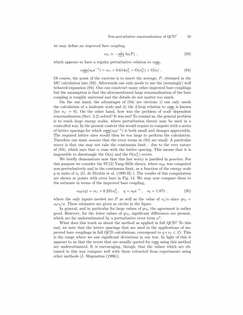
We briefly demonstrate now that this last worry is justified in practice. Forthis purpose we consider the SU(2) Yang-Mills theory, where αSF was computednon-perturbatively and in the continuum limit, as a function of the energy scaleq in units of r0 (G. de Divitiis et al. (1995 II) ). The results of this computationare shown as points with error bars in Fig. 14. We may now compare them tothe estimate in terms of the improved bare coupling,
αSF(q) = α2 + 0.231α32, q = s0a
−1 , s0 = 1.871 , (95)
where the only inputs needed are P as well as the value of r0/a since qr0 =s0r0/a. These estimates are given as circles in the figure.
In general, and in particular for large values of qr0, the agreement is rathergood. However, for the lower values of qr0, significant differences are present,which are far underestimated by a perturbative error term α4.
What does this teach us about the method as applied in full QCD? To thisend, we note that the lattice spacings that are used in the applications of im-proved bare couplings in full QCD calculations, correspond to q ∗ r0 < 15. Thisis the range where we saw significant deviations in our test. In light of this itappears to us that the errors that are usually quoted for αMS using this methodare underestimated. It is encouraging, though, that the values which are ob-tained in this way compare well with those extracted from experiments usingother methods (J. Shigemitsu (1996)).
36 Rainer Sommer
Fig. 14. Test of an improved bare coupling in the SU(2) Yang-Mills theory.
5 Renormalization group invariant quark mass
The computation of running quark masses and the renormalization group invari-ant (RGI) quark mass (Capitani et al. (1997)) proceeds in complete analog tothe computation of α(q). Since we are using a mass-independent renormaliza-tion scheme (cf. Sect. 3.8), the renormalization (and thus the scale dependence)is independent of the flavor of the quark. When we consider “the” running massbelow, any one flavor can be envisaged; the scale dependence is the same for allof them.
The renormalization group equation for the coupling (11) is now accompaniedby one describing the scale dependence of the mass,
q∂m
∂q= τ(g) , (96)
where τ has an asymptotic expansion
τ(g)g→0∼ −g2
d0 + g2d1 + . . .
, d0 = 8/(4π)2 , (97)
with higher order coefficients di, i > 0 which depend on the scheme.Similarly to the Λ-parameter, we may define a renormalization group invari-
ant quark mass, M , by the asymptotic behavior of m,
M = limq→∞
m(2b0g2)−d0/2b
20 . (98)
It is easy to show that M does not depend on the renormalization scheme. Itcan be computed in the SF-scheme and used afterwards to obtain the runningmass in any other scheme by inserting the proper β- and τ -functions in therenormalization group equations.

Non-perturbative renormalization of QCD1 37
Fig. 15. The step scaling function for the quark mass.
To compute the scale evolution of the mass non-perturbatively, we introducea new step scaling function,
σP = ZP(2L)/ZP(L) . (99)
The definition of the corresponding lattice step scaling function and the extrap-olation to the continuum is completely analogous to the case of σ. The onlyadditional point to note is that one needs to keep the quark mass zero through-out the calculation. This is achieved by tuning the bare mass in the lattice actionsuch that the PCAC mass (55) vanishes. At least in the quenched approxima-tion, which has been used so far, this turns out to be rather easy (Luscher et al.(1997 II)).
First results for σP (extrapolated to the continuum) have been obtainedrecently (Capitani et al. (1997)). They are displayed in Fig. 15.
Applying σP and σ recursively one then obtains the series,
m(2−kLmax)/m(2Lmax) , k = 0, 1, . . . , (100)
up to a largest value of k, which corresponds to the smallest g that was con-sidered in Fig. 15. From there on, the perturbative 2-loop approximation to theτ -function and 3-loop approximation to the β-function (in the SF-scheme) maybe used to integrate the renormalization group equations to infinite energy, orequivalently to g = 0. The result is the renormalization group invariant mass,
M = m (2b0g2)−d0/2b
20 exp
−
∫ g
0
dg[ τ(g)β(g) −d0b0g
]
. (101)
In this way, one is finally able to express the running mass m in units of therenormalization group invariant mass, M , as shown in Fig. 16. M has the samevalue in all renormalization schemes, in contrast to the running mass m.
38 Rainer Sommer
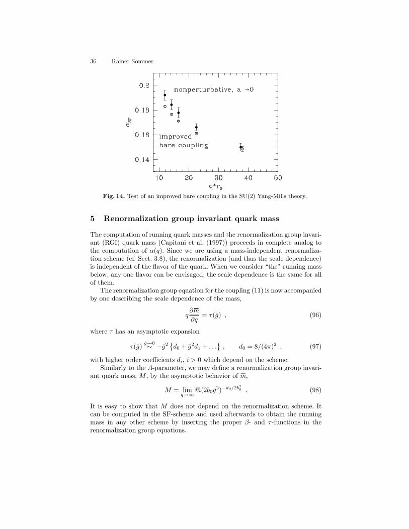
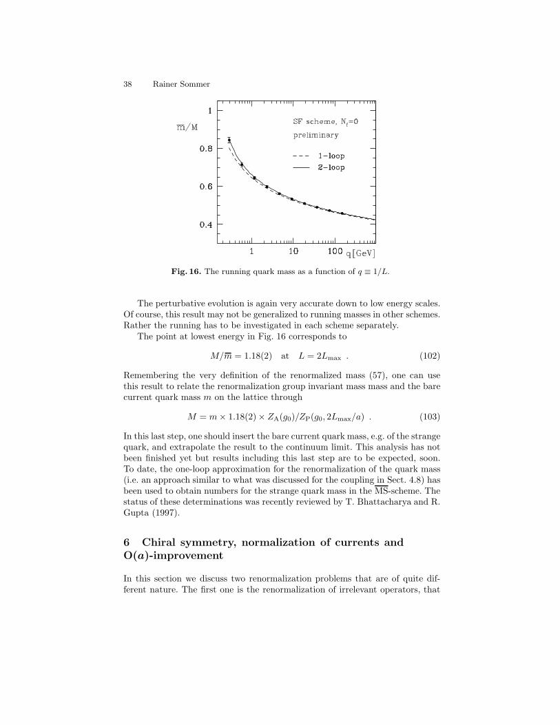
Fig. 16. The running quark mass as a function of q ≡ 1/L.
The perturbative evolution is again very accurate down to low energy scales.Of course, this result may not be generalized to running masses in other schemes.Rather the running has to be investigated in each scheme separately.
The point at lowest energy in Fig. 16 corresponds to
M/m = 1.18(2) at L = 2Lmax . (102)
Remembering the very definition of the renormalized mass (57), one can usethis result to relate the renormalization group invariant mass mass and the barecurrent quark mass m on the lattice through
M = m× 1.18(2)× ZA(g0)/ZP(g0, 2Lmax/a) . (103)
In this last step, one should insert the bare current quark mass, e.g. of the strangequark, and extrapolate the result to the continuum limit. This analysis has notbeen finished yet but results including this last step are to be expected, soon.To date, the one-loop approximation for the renormalization of the quark mass(i.e. an approach similar to what was discussed for the coupling in Sect. 4.8) hasbeen used to obtain numbers for the strange quark mass in the MS-scheme. Thestatus of these determinations was recently reviewed by T. Bhattacharya and R.Gupta (1997).
6 Chiral symmetry, normalization of currents andO(a)-improvement
In this section we discuss two renormalization problems that are of quite dif-ferent nature. The first one is the renormalization of irrelevant operators, that
Non-perturbative renormalization of QCD1 39
are of interest in the systematic O(a) improvement of Wilson’s lattice QCD asmentioned in Sect. 1.4. The second one is the finite normalization of isovectorcurrents (cf. Sect. 1.2). They are discussed together, here, because – at least to alarge extent – they can be treated with a proper application of chiral Ward iden-tities. The possibility to use chiral Ward identities to normalize the currents hasfirst been discussed by Bochicchio et al. (1985), Maiani and Martinelli (1986).Earlier numerical applications can be found in Martinelli et al. (1993), Pacielloet al. (1994), Henty et al. (1995) and a complete calculation is described be-low (Luscher et al. (1997 I)). We also sketch the application of chiral Ward iden-tities in the computation of the O(a)-improved action and currents (Luscher etal. (1996), Luscher and Weisz (1996), Luscher et al. (1997 I)).
Before going into the details, we would like to convey the rough idea of theapplication of chiral Ward identities. For simplicity we again assume an isospindoublet of mass-degenerate quarks. Imagine that we have a regularization ofQCD which preserves the full SU(2)V×SU(2)A flavor symmetry as it is presentin the continuum Lagrangian of mass-less QCD. In this theory we can derivechiral Ward identities, e.g. in the Euclidean formulation of the theory. Thesethen provide exact relations between different correlation functions. Immediateconsequences of these relations are that the currents (5) do not get renormalized(ZA = ZV = 1) and the quark mass does not have an additive renormalization.
Lattice QCD does, however, not have the full SU(2)V×SU(2)A flavor symme-try for finite values of the lattice spacing and in fact no regularization is knownthat does. Therefore, the Ward identities are not satisfied exactly. We do, how-ever, expect that the renormalized correlation functions obey the same Wardidentities as before – up to O(a) corrections that vanish in the continuum limit.Therefore we may impose those Ward identities for the renormalized currents,to fix their normalizations.
Furthermore, following Symanzik, it suffices to a add a few local irrelevantterms to the action and to the currents in order to obtain an improved latticetheory, where the continuum limit is approached with corrections of order a2.The coefficients of these terms can be determined by imposing improvementconditions. For example one may require certain chiral Ward identities to bevalid at finite lattice spacing a.
6.1 Chiral Ward identities
For the moment we do not pay attention to a regularization of the theory andderive the Ward identities in a formal way. As mentioned above these identitieswould be exact in a regularization that preserves chiral symmetry. To derive theWard identities, one starts from the path integral representation of a correlationfunction and performs the change of integration variables
ψ(x) → eiτa
2 [ǫaA(x)γ5+ǫa
V(x)]ψ(x)
= ψ(x) + iǫaA(x)δaAψ(x) + iǫaV(x)δaVψ(x) ,
40 Rainer Sommer
ψ(x) → ψ(x)eiτa
2 [ǫaA(x)γ5−ǫa
V(x)]
= ψ(x) + iǫaA(x)δaAψ(x) + iǫaV(x)δaVψ(x) , (104)
where we have taken ǫaA(x), ǫaV(x) infinitesimal and introduced the variations
δaVψ(x) = 12τ
aψ(x), δaVψ(x) = −ψ(x)12τ
a ,
δaAψ(x) = 12τ
aγ5ψ(x), δaAψ(x) = ψ(x)γ512τ
a . (105)
The Ward identities then follow from the invariance of the path integral rep-resentation of correlation functions with respect to such changes of integrationvariables. They obtain contributions from the variation of the action and thevariations of the fields in the correlation functions. In Sect. 6.3 we will need thevariations of the currents,
δaVVbµ (x) = −iǫabcV cµ (x), δaAV
bµ (x) = −iǫabcAcµ(x),
δaVAbµ(x) = −iǫabcAcµ(x), δaAA
bµ(x) = −iǫabcV cµ (x) . (106)
They form a closed algebra under these variations.Since this is convenient for our applications, we write the Ward identities in
an integrated form. Let R be a space-time region with smooth boundary ∂R.Suppose Oint and Oext are polynomials in the basic fields localized in the interiorand exterior of R respectively. The general vector current Ward identity thenreads
∫
∂R
dσµ(x)⟨V aµ (x)OintOext
⟩= −〈(δaVOint)Oext〉 , (107)
while for the axial current one obtains∫
∂R
dσµ(x)⟨Aaµ(x)OintOext
⟩= −〈(δaAOint)Oext〉 (108)
+2m
∫
R
d4x 〈P a(x)OintOext〉 .
The integration measure dσµ(x) points along the outward normal to the surface∂R and the pseudo-scalar density P a(x) is defined by
P a(x) = ψ(x)γ512τ
aψ(x) . (109)
We may also write down the precise meaning of the PCAC-relation (55). Itis (108) in a differential form,
⟨[∂µA
aµ(x) − 2mP a(x)
]Oext
⟩= 0 , (110)
where now Oext may have support everywhere but at the point x.Going through the same derivation in the lattice regularization, one finds
equations of essentially the same form as the ones given above, but with addi-tional terms (Bochicchio et al. (1985)). At the classical level these terms are of
Non-perturbative renormalization of QCD1 41
order a. More precisely, in (110) the important additional term originates fromthe variation of the Wilson term, aψ∇∗
µ∇µψ, and is a local field of dimension 5.Such O(a)-corrections are present in any observable computed on the lattice andare no reason for concern. However, as is well known in field theory, such opera-tors mix with the ones of lower and equal dimensions when one goes beyond theclassical approximation. In the present case, the dimension five operator mixesamongst others also with ∂µA
aµ(x) and P a(x). This means that part of the classi-
cal O(a)-terms turn into O(g20) in the quantum theory. The essential observation
is now that this mixing can simply be written in the form of a renormalizationof the terms that are already present in the Ward identities, since all dimensionthree and four operators with the right quantum number are already there.
We conclude that the identities, which we derived above in a formal manner,are valid in the lattice regularization after
– replacing the bare fields A, V, P and quark mass m0 by renormalized ones,where one must allow for the most general renormalizations,
(AR)aµ = ZAAaµ , (VR)aµ = ZVV
aµ ,
(PR)a = ZPPa , mR = Zmmq , mq = m0 −mc ,
– allowing for the usual O(a) lattice artifacts.
Note that the additive quark mass renormalization mc diverges like O(g20/a) for
dimensional reasons.
As a result of this discussion, the formal Ward identities may be used todetermine the normalizations of the currents. We discuss this in more detail inSect. 6.3 and first explain the general idea how one can use the Ward identitiesto determine improvement coefficients.
6.2 O(a)-improvement
We refer the reader to Luscher et al. (1996) for a thorough discussion of O(a)-improvement and to Sommer (1997) for a review. Here, we only sketch howchiral Ward identities may be used to determine improvement coefficients non-perturbatively.
The form of the improved action and the improved composite fields is deter-mined by the symmetries of the lattice action and in addition the equations ofmotion may be used to reduce the set of operators that have to be considered(Luscher and Weisz (1985)). For O(a)-improvement, the improved action con-tains only one additional term, which is conveniently chosen as (Sheikholeslamiand Wohlert (1985))
δS = a5∑
x
cswψ(x) i4σµν Fµν(x)ψ(x), (111)
42 Rainer Sommer
with Fµν a lattice approximation to the gluon field strength tensor Fµν and oneimprovement coefficient csw. The improved and renormalized currents may bewritten in the general form
(VR)aµ = ZV(1 + bVamq)V aµ + acV
12 (∂ν + ∂∗ν )T
aµν
,
T aµν(x) = iψσµν12τ
aψ(x)
(AR)aµ = ZA(1 + bAamq)Aaµ + acA
12 (∂µ + ∂∗µ)P
a,
(PR)a = ZP(1 + bPamq)Pa . (112)
(∂µ and ∂∗µ are the forward and backward lattice derivatives, respectively.)
Improvement coefficients like csw and cA are functions of the bare coupling,g0, and need to be fixed by suitable improvement conditions. One considers purelattice artifacts, i.e. combinations of observables that are known to vanish inthe continuum limit of the theory. Improvement conditions require these latticeartifacts to vanish, thus defining the values of the improvement coefficients as afunction of the lattice spacing (or equivalently as a function of g0).
In perturbation theory, lattice artifacts can be obtained from any (renormal-ized) quantity by subtracting its value in the continuum limit. The improvementcoefficients are unique.
Beyond perturbation theory, one wants to determine the improvement coef-ficients by MC calculations and it requires significant effort to take the contin-uum limit. It is therefore advantageous to use lattice artifacts that derive from asymmetry of the continuum field theory that is not respected by the lattice reg-ularization. One may require rotational invariance of the static potential V (r),e.g.
V (r = (2, 2, 1)r/3) − V (r = (r, 0, 0)) = 0 ,
or Lorenz invariance,
[E(p)]2 − [E(0)]2 − p2 = 0 ,
for the momentum dependence of a one-particle energy E.
For O(a)-improvement of QCD it is advantageous to require instead thatparticular chiral Ward identities are valid exactly.9
In somewhat more detail, the determination of csw and cA is done as follows.We define a bare current quark mass, m, viz.
m ≡⟨[∂µ(AI)
aµ(x)
]Oext
⟩
2 〈P a(x)Oext〉, (AI)
aµ = Aaµ + acA
12 (∂µ + ∂∗µ)P
a . (113)
9 As a consequence of the freedom to choose improvement conditions, the resultingvalues of improvement coefficients such as csw, cA depend on the exact choices made.The corresponding variation of csw, cA is of order a. There is nothing wrong withthis unavoidable fact, since an O(a) variation in the improvement coefficients onlychanges the effects of order a2 in physical observables computed after improvement.
Non-perturbative renormalization of QCD1 43
When all improvement coefficients have their proper values, the renormalizedquark mass, defined by the renormalized PCAC-relation, is related to m by
mR =ZA(1 + bAamq)
ZP(1 + bPamq)m+ O(a2) . (114)
We now choose 3 different versions of (113) by different choices for Oext and/orboundary conditions and obtain 3 different values of m, denoted by m1,m2,m3.Since the prefactor in front of m in (114) is just a numerical factor, we mayconclude that all mi have to be equal in the improved theory up to errors oforder a2. csw and cA may therefore be computed by requiring
m1 = m2 = m3 . (115)
This simple idea has been used to compute csw and cA as a function of g0 inthe quenched approximation (Luscher et al. (1997 II)). In the theory with twoflavors of dynamical quarks, csw has been computed in this way (Jansen andSommer (1997)). The improvement coefficient for the vector current, cV, maybe computed through a different chiral Ward identity (Guagnelli and Sommer(1997)).
6.3 Normalization of isovector currents
Although the numerical results, which we will show below, have been obtainedafter O(a) improvement, the normalization of the currents as it is described,here, is applicable in general. Without improvement one just has to rememberthat the error terms are of order a, instead of a2. For the following, we set thequark mass (as calculated from the PCAC-relation) to zero.
Normalization condition for the vector current. Since the isospin sym-metry of the continuum theory is preserved on the lattice exactly, there existsalso an exactly conserved vector current. This means that certain specific Ward-identities for this current are satisfied exactly and fix it’s normalization automat-ically. It is, however, convenient to use the improved vector current introducedabove, which is only conserved up to cutoff effects of order a2. Its normalizationis hence not naturally given and we must impose a normalization condition tofix ZV. Our aim in the following is to derive such a condition by studying theaction of the renormalized isospin charge on states with definite isospin quantumnumbers.
The matrix elements that we shall consider are constructed in the SF using(the lattice version of) the boundary field products introduced in (58) to createinitial and final states that transform according to the vector representation ofthe exact isospin symmetry. The correlation function
fRV (x0) =
a3
6L6
∑
x
iǫabc〈O ′a(VR)b0(x)Oc〉 (116)
44 Rainer Sommer
can then be interpreted as a matrix element of the renormalized isospin chargebetween such states. The properly normalized charge generates an infinitesimalisospin rotation and after some algebra one finds that the correlation functionmust be equal to
f1 = − 1
3L6〈O ′aOa〉 (117)
up to corrections of order a2. The O(a) counter-term appearing in the definition(112) of the improved vector current does not contribute to the correlation func-tion fR
V (x0). So if we introduce the analogous correlation function for the barecurrent,
fV(x0) =a3
6L6
∑
x
iǫabc〈O ′aV b0 (x)Oc〉, (118)
it follows from (117) that
ZVfV(x0) = f1 + O(a2). (119)
By evaluating the correlation functions f1 and fV(x0) through numerical simu-lation one is thus able to compute the normalization factor ZV.
Normalization condition for the axial current. To derive a normalizationcondition for ZA, we consider (108) (for m = 0) and choose Oint to be the axialcurrent at some point y in the interior of R. The resulting identity,
∫
∂R
dσµ(x)⟨Aaµ(x)A
bν (y)Oext
⟩= iǫabc 〈V cν (y)Oext〉 , (120)
is valid for any type of boundary conditions and space-time geometry, but wenow assume Schrodinger functional boundary conditions as before. A convenientchoice of the region R is the space-time volume between the hyper-planes atx0 = y0 ± t. On the lattice we then obtain the relation10
a3∑
x
ǫabc⟨[(AR)a0(y0 + t,x) − (AR)a0(y0 − t,x)](AR)b0(y)Oext
⟩
= 2i 〈(VR)c0(y)Oext〉 + O(a2) . (121)
After summing over the spatial components of y, and using the fact that theaxial charge is conserved at zero quark mass (up to corrections of order a2),(121) becomes
a6∑
x,y
ǫabc⟨(AR)a0(x)(AR)b0(y)Oext
⟩= a3
∑
y
i 〈(VR)c0(y)Oext〉 + O(a2), (122)
10 In the context of O(a)-improvement it has been important here that the fields in thecorrelation functions are localized at non-zero distances from each other. Since thetheory is only on-shell improved, one would otherwise not be able to say that theerror term is of order a2 (cf. sect. 2 of Luscher et al. (1996)).
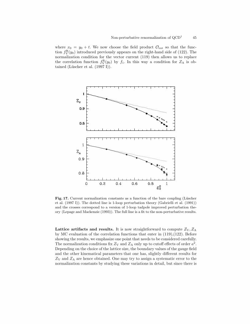
Non-perturbative renormalization of QCD1 45
where x0 = y0 + t. We now choose the field product Oext so that the func-tion fR
V (y0) introduced previously appears on the right-hand side of (122). Thenormalization condition for the vector current (119) then allows us to replacethe correlation function fR
V (y0) by f1. In this way a condition for ZA is ob-tained (Luscher et al. (1997 I)).
Fig. 17. Current normalization constants as a function of the bare coupling (Luscheret al. (1997 I)). The dotted line is 1-loop perturbation theory (Gabrielli et al. (1991))and the crosses correspond to a version of 1-loop tadpole improved perturbation the-ory (Lepage and Mackenzie (1993)). The full line is a fit to the non-perturbative results.
Lattice artifacts and results. It is now straightforward to compute ZV, ZA
by MC evaluation of the correlation functions that enter in (119),(122). Beforeshowing the results, we emphasize one point that needs to be considered carefully.The normalization conditions fix ZV and ZA only up to cutoff effects of order a2.Depending on the choice of the lattice size, the boundary values of the gauge fieldand the other kinematical parameters that one has, slightly different results forZV and ZA are hence obtained. One may try to assign a systematic error to thenormalization constants by studying these variations in detail, but since there is
46 Rainer Sommer
no general rule as to which choices of the kinematical parameters are consideredto be reasonable, such error estimates are bound to be rather subjective.
It is therefore better to deal with this problem by defining the normalizationconstants through a particular normalization condition. The physical matrixelements of the renormalized currents that one is interested in must then becalculated for a range of lattice spacings so as to be able to extrapolate the datato the continuum limit. The results obtained in this way are guaranteed to beindependent of the chosen normalization condition, because any differences inthe normalization constants of order a2 extrapolate to zero together with thecutoff effects associated with the matrix elements themselves.
Note that a “particular normalization condition” means that apart fromchoosing the boundary values and geometry of the SF, one has to keep thesize of the SF-geometry fixed in physical units, for example
L/r0 = const. (123)
As shown in Fig. 17, the current normalizations can be obtained with goodprecision (in the quenched approximation) after taking all of these points intoaccount (Luscher et al. (1997 I)).
Coming back to our motivation Sect. 1.2, the results in Fig. 17 now allow forthe calculation of matrix elements of the weak currents involving light quarkswithout any perturbative uncertainties.
7 Summary, Conclusions
We have shown how QCD needs to be renormalized non-perturbatively in orderto obtain unambiguous predictions that can be compared with experiments.Once a non-perturbative definition and calculational technique is available, itis in principle quite simple to perform renormalization non-perturbatively. Inpractice, the problem has to be treated with care.
The only presently available definition is lattice QCD with MC simulations asthe calculational tool to get predictions. In this case, straightforward solutions tothe renormalization problem face a serious difficulty: the theory must be treatedat various different energy scales simultaneously, which is an extremely hard(impossible?) task for a MC simulation. To circumvent this difficulty, Luscher,Weisz and Wolff have introduced the recursive finite size technique, where oneconnects low and high energies recursively in small steps. We have shown, howthis idea can be put into practice in QCD using the Schrodinger functional asa second technical tool. In the theory without dynamical quarks, these meth-ods have been shown to allow for the computation of short distance parameterslike ΛMS and the renormalization group invariant quark mass with completelycontrolled errors! From the practical point of view, the non-perturbative renor-malization of other quantities, such as the ∆s = 2 operator, still have to beinvestigated, but no new difficulties are expected to appear. It is therefore plau-sible that the renormalization problem can be solved for many specific cases –

Non-perturbative renormalization of QCD1 47
and with good accuracy. It should not remain unmentioned, however, that inpractice each renormalization problem has to be considered separately. Certainproblems may turn out to be significantly more difficult to solve than the onesdiscussed in the lectures.
We also sketched, how Symanzik improvement can be implemented in anon-perturbative way, reducing the leading lattice artifacts from linear in a toquadratic in a (O(a)-improvement). For light quarks, such a project has alreadybeen done carried out. As a result, significant progress in lattice QCD is expectedfrom the use of O(a)-improved QCD.
Acknowledgment. I am grateful to the organizers of this school for composingan interesting programme and directing the school with excellence. I would liketo thank my friends in the ALPHA-collaboration for all they taught me and forthe most enjoyable and fruitful collaboration; special thanks go to J. Heitger andF. Jegerlehner for critical comments on the manuscript. I further thank DESYfor allocating computer time for the ALPHA-project, which was essential for anumber of the numerical investigations that were discussed in these lectures.
References
K. G. Wilson, Phys. Rev. D10 (1974) 2445D. Weingarten, Lectures at this schoolB. Meyer and C. Smith, Phys. Lett. 123B (1983) 62G. Martinelli and Zhang Yi-Cheng, Phys. Lett. 123B (1983) 433; ibid. 125B (1983) 77R. Groot, J. Hoek and J. Smit, Nucl. Phys. B237 (1984) 111E. Gabrielli et al., Nucl. Phys. B362 (1991) 475A. Borrelli, C. Pittori, R. Frezzotti and E. Gabrielli, Nucl. Phys. B409 (1993) 382M. Bochicchio, L. Maiani, G. Martinelli, G.C. Rossi and M. Testa, Nucl. Phys. B262
(1985) 331L. Maiani and G. Martinelli, Phys. Lett. B178 (1986) 265M. Luscher, S. Sint, R. Sommer and H. Wittig, Nucl. Phys. B491 (1997) 344P. Franzini, Phys. Rep. C173 (1989) 1;L. Maiani, G. Martinelli, G.C. Rossi and M. Testa, Nucl. Phys. B289 (1987) 505S. Aoki et al., Nucl. Phys. (Proc. Suppl.) 53 (1997) 349K. Symanzik, Some topics in quantum field theory, in: Mathematical problems in theo-
retical physics, eds. R. Schrader et al., Lecture Notes in Physics, Vol. 153 (Springer,New York, 1982)
K. Symanzik, Nucl. Phys. B226 (1983) 187 and 205G.P. Lepage in Schladming 1996, Perturbative and non-perturbative aspects of quan-
tum field theory, hep-lat/9607076R. Sommer, O(a)-improved lattice QCD, hep-lat/9705026F. Niedermayer, Nucl. Phys. (Proc. Suppl.) 53 (1997) 56G. Grunberg, Phys. Rev. D29 (1984) 2315I. Montvay and G. Munster, Quantum Fields on a Lattice, (Cambridge, New York,
1994)C. Michael, Phys. Lett. B283 (1992) 103S. P. Booth et al. (UKQCD Collab.), Phys. Lett. B294 (1992) 385
48 Rainer Sommer
G. S. Bali and K. Schilling, Phys. Rev. D47 (1993) 661M. Luscher, P. Weisz and U. Wolff, Nucl. Phys. B359 (1991) 221A. Gonzales-Arroyo, J. Jurkiewicz and C.P. Kothals-Altes, Ground state metamorpho-
sis for Yang-Mills fields on a finite periodic lattice, in: Structural elements in particlephysics and statistical mechanics, ed. J. Honerkamp and K. Pohlmeyer (Plenum, NewYork, 1983)
M. Luscher, Nucl. Phys. B219 (1983) 233G. ’t Hooft, Nucl. Phys. B153 (1979) 141; Commun. Math. Phys. 81 (1981) 267P. van Baal, Commun. Math. Phys. 92 (1983) 1M. Luscher and P. Weisz, Phys. Lett. 158B (1985) 250; Nucl. Phys. B266 (1986) 309M. Luscher, R. Narayanan, P. Weisz and U. Wolff, Nucl. Phys. B384 (1992) 168M. Luscher, R. Sommer, P. Weisz and U. Wolff, Nucl. Phys. B389 (1993) 247, Nucl.
Phys. B413 (1994) 481S. Sint, Nucl. Phys. B421 (1994) 135, Nucl. Phys. B451 (1995) 416K. Jansen, C. Liu, M. Luscher, H. Simma, S. Sint, R. Sommer, P. Weisz and U. Wolff,
Phys. Lett. B372 (1996) 275G. Martinelli, C. Pittori, C.T. Sachrajda, M. Testa and A. Vladikas, Nucl. Phys. B445
(1994) 81A. Donini, G. Martinelli, C.T. Sachrajda, M. Talevi and A. Vladikas, Phys. Lett. B360
(1995) 83H. Oelrich et al., hep-lat/9710052G. de Divitiis et al., Nucl. Phys. B422 (1994) 382G. de Divitiis et al., Nucl. Phys. B433 (1995) 390G. de Divitiis et al., Nucl. Phys. B437 (1995) 447K. Symanzik, Nucl. Phys. B190 [FS3] (1981) 1M. Luscher, Nucl. Phys. B254 (1985) 52R. Narayanan, and U. Wolff, Nucl. Phys. B444 (1995) 425A. Bode, hep-lat/9710043M. Luscher and P. Weisz, Phys. Lett. B349 (1995) 165R. Sommer, Nucl. Phys. B411 (1994) 839E. Eichten et al., Phys. Rev. D21 (1980) 203A. Martin, Phys. Lett. B93 (1980) 338C. Quigg and J.L. Rosner, Phys. Lett. B71 (1977) 153H. Wittig (UKQCD collab.), Nucl. Phys. B (Proc. Suppl.) 42 (1995) 288;
H. Wittig (UKQCD collab.), unpubl.S. Sint and R. Sommer, Nucl. Phys. B465 (1996) 71W. Fishler, Nucl. Phys. B129 (1977) 157A. Billoire, Phys. Lett. B92 (1980)M. Peter, hep-ph/9702245A.X. El-Khadra, G. Hockney, A.S. Kronfeld, and P.B. Mackenzie, Phys. Rev. Lett. 69
(1992) 729J. Shigemitsu, Nucl. Phys. B (Proc. Suppl.) 53 (1997) 16C. Davies, Lectures at this schoolG. P. Lepage and P. Mackenzie, Phys. Rev. D48 (1993) 2250G. Parisi, in: High-Energy Physics — 1980, XX. Int. Conf., Madison (1980), ed. L.
Durand and L. G. Pondrom (American Institute of Physics, New York, 1981)S. Capitani et al., hep-lat/9709125T. Bhattacharya and R. Gupta, talk at the International Symposium on Lattice Field
Theory, 21−27 July 1997, Edinburgh, Scotland
Non-perturbative renormalization of QCD1 49
G. Martinelli, S. Petrarca, C. T. Sachrajda and A. Vladikas, Phys. Lett. B311 (1993)241, E: B317 (1993) 660
M. L. Paciello, S. Petrarca, B. Taglienti and A. Vladikas, Phys. Lett. B341 (1994) 187D. S. Henty, R. D. Kenway, B. J. Pendleton and J.I. Skullerud, Phys. Rev. D51 (1995)
5323M. Luscher, S. Sint, R. Sommer and P. Weisz, Nucl. Phys. B478 (1996) 365M. Luscher and P. Weisz, Nucl. Phys. B479 (1996) 429M. Luscher, S. Sint, R. Sommer, P. Weisz and U. Wolff, Nucl. Phys. B491 (1997) 323M. Luscher and P. Weisz, Commun. Math. Phys. 97 (1985) 59, E: Commun. Math.
Phys. 98 (1985) 433B. Sheikholeslami and R. Wohlert, Nucl. Phys. B259 (1985) 572K. Jansen and R. Sommer, hep-lat / 9709022M. Guagnelli and R. Sommer, hep-lat / 9709022