Embed Size (px)
Citation preview
Coastal Engineering 56 (2009) 960–969
Contents lists available at ScienceDirect
Coastal Engineering
j ourna l homepage: www.e lsev ie r.com/ locate /coasta leng
Effect of bed roughness on turbulent boundary layer and net sediment transportunder asymmetric waves
Suntoyo a,⁎, Hitoshi Tanaka b
a Department of Ocean Engineering, Faculty of Marine Technology, Institut Teknologi Sepuluh Nopember (ITS), Surabaya 60111, Indonesiab Department of Civil Engineering, Tohoku University, 6-6-06 Aoba, Sendai 980-8579, Japan
⁎ Corresponding author. Tel./fax: +62 31 5928105.E-mail addresses: [email protected] (Suntoyo),
[email protected] (H. Tanaka).
0378-3839/$ – see front matter © 2009 Elsevier B.V. Adoi:10.1016/j.coastaleng.2009.06.005
a b s t r a c t
a r t i c l e i n f oArticle history:Received 7 April 2008Received in revised form 5 May 2009Accepted 8 June 2009Available online 10 July 2009
Keywords:Turbulent boundary layersShallow waterAsymmetric waveBed-load transport
This paper presents an investigation of the roughness effects in the turbulent boundary layer for asymmetricwaves by using the baseline (BSL) k–ω model. This model is validated by a set of the experimental data withdifferent wave non-linearity index, Ni (namely, Ni=0.67, Ni=0.60 and Ni=0.58). It is further used tosimulate asymmetric wave velocity flows with several values of the roughness parameter (am/ks) whichincrease gradually, namely from am/ks=35 to am/ks=963. The effect of the roughness tends to increase theturbulent kinetic energy and to decrease the mean velocity distribution in the inner boundary layer, whereasin the outer boundary layer, the roughness alters the turbulent kinetic energy and the mean velocitydistribution is relatively unaffected. A new simple calculation method of bottom shear stress based onincorporating velocity and acceleration terms is proposed and applied into the calculation of the rate of bed-load transport induced by asymmetric waves. And further, the effect of bed roughness on the bottom shearstress and bed-load sediment transport under asymmetric waves is examined with the turbulent model, thenewly proposed method, and the existing calculation method. It is found that the higher roughness elementsincrease the magnitude of bottom shear stress along a wave cycle and consequently, the potential netsediment transport rate. Moreover, the wave non-linearity also shows a big impact on the bottom shear stressand the net sediment transport.
© 2009 Elsevier B.V. All rights reserved.
1. Introduction
Bed-load transport generally depends on the bottom shear stressand the near-bottom velocity of waves. The wave boundary layer andthe bottom friction studies associated with sediment movementinduced bywave motion for sinusoidal waves have been conducted bymany researchers (e.g., Sawamoto and Yamashita (1986), Ahilan andSleath (1987), Fredsøe and Deigaard (1992)). Studies involving thesediment transport rate under sinusoidal waves have shown that thenet sediment transport over a complete wave cycle is zero. In reality,however, waves are non-linear having asymmetry of the near-bottomvelocity between wave crest and trough and also the asymmetricacceleration actualized on the skew waves in which the net sedimenttransport over a complete wave cycle can be non-zero. Dibajnia andWatanabe (1992) investigated the initiation of sheet flow underasymmetric oscillation obtained from the first-order cnoidal wavetheory. They measured the net sheet sand transport rate underasymmetric oscillations superimposed with steady currents, andpresented the sediment transport formula for estimating the nettransport rate and its direction without the use of the bottom shear
ll rights reserved.
stress and Shield's parameter. The effect of wave asymmetry on sheetflow has been studied by Wilson et al. (1995), who obtained therelationship among the friction factor, the initiation of sheet flow andthe net bed-load transport produced by asymmetric waves. Al-Salem(1993) presented detailed boundary layer measurements in variousconditions showing that although the phase difference between thenear-bed sediment concentration and oscillatory flow velocities is notan important factor, they are closely coupled in time. However,Janssen et al. (2002) have shown that even in the sheet flow, the phasedifference between the sediment concentration and the near-bedvelocities could become an important factor affecting the netsediment transport. Black and Vincent (2001) have investigated anintra-wave sediment suspension using high-resolution field measure-ments and numerical hydrodynamic and sediment model within120 mm of a plane seabed under natural asymmetric waves. Theyshow that wave asymmetry plays an important role in suspension bycreating oppositely directed current shear near the bed around thetime of flow reversal, predominantly during the decelerating phase asalso shown by Savioli and Justesen (1997).
An appearance of roughness often occurs in the seabed. The shapeof the near-bed wave orbital velocity is a key parameter influencingcross-shore sediment transport under breaking and near-breakingwaves. Waves may be highly asymmetric or non-linear whenpropagating into shallow water. Therefore, the turbulent boundary

Fig. 1. Diagram of a cnoidal wave.
961Suntoyo, H. Tanaka / Coastal Engineering 56 (2009) 960–969
layer created under asymmetric waves over in varying bed roughnessmay exceed the wave boundary layer behavior in the near shore. It isenvisaged that the higher roughnesswould yield higher turbulent kineticenergy and bottom shear stress that will increase the impact on thesediment transport near shore. Cotton and Stansby (2000) investigatedthe effect of wave non-linearity onwave friction factor and wave energydissipation factor for rough-bed turbulent boundary layer using severalrelative values of the roughness parameter, am/ks=30, 100 and 1000.Here, ks is Nikuradse's equivalent roughness and am=Uc/σ is the orbitalamplitude of fluid just above the boundary layer or near-bed semi-excursion, where, Uc is the velocity at wave crest and σ is the angularfrequency. The boundary layer computation is based on a k–ε turbulencemodel showing that the energy dissipation rates reduce sharply undernon-linear condition. The wave friction factor and the wave energydissipation factor increase due to decreases in the roughness parameter,am/ks. Briggs et al. (2002) have investigated the characteristic of wave-formed sediment ripples in nature through stereo photography and atechnique using a conductivity system. The results show that thesediment bed changes from isotropic to anisotropic. Recently, Daviset al. (2004) have developed a new method that models the changes awave-formed rippled sediment bed undergoes as it actively evolvesbetween two given equilibrium states due to change in surface wavecondition. They show that the estimation of the rate at which rippledsediment beds evolve under a variable sea state has the potential to leadto significant improvement in the way transition and hence bottomroughness is approximated in coastal wavemodels. Recently, Dixen et al.(2008) investigated the wave boundary layer over a stone-covered bedwith a rather small roughness parameter, in the range of am/ks=0.6–3.0.The results show that the turbulent boundary layer is not extremelysensitive to the packing pattern, the packing density, the number oflayers, or the surface roughness of the roughness element. Moreover, thefriction factor for small values of am/ks=0.6–3.0 is not a constant value,which is contrary to suggestions of some previous investigators.
Tanaka et al. (1998) derived an analytical solution for laminarbottom boundary layer under cnoidal waves. Excellent agreementwith experimental data has been obtained. The fundamentalcharacteristics under an asymmetric boundary layer, such as velocityprofile, bottom shear stress and boundary layer thickness, showdifferences from those characteristics under symmetric waves.Recently, Sana et al. (2006) have studied the boundary layer behaviorunder asymmetric waves from laminar to turbulent flow regimes witha low Reynolds number k–ε model that they validated withexperimental data. A stability diagram for asymmetric wave boundarylayers was obtained and the demarcation lines between differentregimes of flowwere given in terms of Reynolds number and degree ofasymmetry. However, these results have not been validated withexperimental data for high Reynolds number. More recently, Lin andZhang (2008) simulated the laminar boundary layer under variouswaves (i.e., linear, Stokes, cnoidal and solitary waves) using the three-dimensional hydrodynamic numerical model. The proposed modelprovided consistently accurate results for all types of wave-inducedlaminar boundary layer flows. However, the characteristics of theturbulent boundary layer flow with varying of the bed roughnessunder asymmetric waves have not been simulated, yet.
Tanaka (1998) estimated the bottom shear stress under non-linearwaves with modified stream function theory and proposed a formulato predict bed-load transport outside the surf zone in which theacceleration effect plays an important role. Madsen (1991) has shownthat although sediment particles react almost instantaneously to thefluid forces, the particle acceleration forces in oscillatory flow can beneglected in the sand particle range of 0.2–2.0 mm. However,Watanabe and Sato (2004) have shown that the fluid accelerationeffect on the bed shear stress leads to a small net transport in the caseof skewwaves, even if the crest and trough orbital velocities are equal.Recently, Nielsen (2002), Nielsen and Callaghan (2003) and Nielsen(2006) applied a modified version of the bottom shear stress formula
based on incorporating the velocity and acceleration terms proposedby Nielsen (1992) and applied it to predict sediment transport ratewith assorted sediment transport experimental data. However, theyhave shown that the phase difference between free stream velocityand bottom shear stress used to evaluate the sediment transport canvary from 40° to 51°. Whereas, many researchers (e.g., Fredsøe andDeigaard, 1992; Tanaka and Thu, 1994) have shown that the phasedifference in laminar flow is 45°, and drops from 45° to about 10° inthe turbulent flow case. However, it is possible that phase differencesmore than 45° may occur at some depth below the undisturbed level,whereas the phase difference just above undisturbed level may beonly 10–20° (Sleath,1987; Dick and Sleath,1991). These authors foundthat the phase difference and shear stress were dependent on thecross-stream distance from the bed, z for a mobile, rough bed.
More recently, Suntoyo et al. (2008) have studied the characteristicsof the turbulentboundary layer under saw-toothwaves over a roughbedthrough laboratory and numerical experiments. A good agreementbetween numerical and experimental data for mean velocity distribu-tion, turbulent intensity and bottom shear stress was obtained. A newcalculationmethod for calculating bottom shear stress under saw-toothwaves has been proposed based on velocity and acceleration termswhere the effect of wave skewness is incorporated using a factor ac,which is determined empirically from experimental data and thebaseline (BSL) k–ωmodel results. The newmethod has shown the bestagreement with the experimental data along a wave cycle for all saw-tooth wave cases in comparison with the existing calculation methods.Moreover, the new method of bottom shear stress calculation wasapplied to the net sediment transport experimental data under sheetflow conditions by Watanabe and Sato (2004) and a good agreementwas found. However, the proposedmodel has a limitation in that it doesnot simulate the sediment suspension.
In the present paper, the effect of the roughness in the turbulentboundary layer for asymmetricwaves is investigated by using the BSL k–ωmodel. This model is validated by a set of the experimental data withdifferent values for the wave non-linearity index, Ni (namely, Ni=0.67,Ni=0.60 and Ni=0.58). It is further used to simulate asymmetric wavevelocity flows with several values of the roughness parameter (am/ks)that increase gradually from am/ks=35 to am/ks=963. The effect of theroughness on the mean velocity, bottom shear stress and the turbulentkinetic energy is examined. Moreover, a new calculation method ofbottom shear stress based on incorporating both velocity and accelera-tion terms is proposed and applied to the calculation of the bed-loadtransport rate induced by asymmetric waves. And further, the effect ofbed roughness on the bottom shear stress and bed-load sedimenttransport is examined with the turbulent model, the proposed method,and the existing calculation method.
2. Experimental study
Experiments were performed for three cases under cnoidal wavesto represent the asymmetric waves in an oscillation tunnel using air astheworking fluid. A cnoidal wave is defined in Fig. 1. The experimental
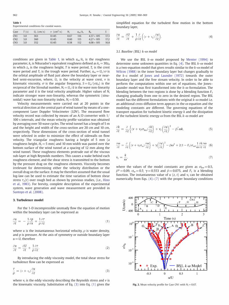
Table 1Experimental conditions for cnoidal waves.
Case T (s) Uc (cm/s) v (cm2/s) Ni am/ks Re S
CN1 3.0 363 0.145 0.67 116 4.37×10⁵ 17.3CN2 3.0 360 0.145 0.60 115 4.27×10⁵ 17.2CN3 3.0 352 0.145 0.58 112 4.08×10⁵ 16.8
Fig. 2. Mean velocity profile for Case CN1 with Ni=0.67.
962 Suntoyo, H. Tanaka / Coastal Engineering 56 (2009) 960–969
conditions are given in Table 1, in which am/ks is the roughnessparameter, ks is Nikuradse's equivalent roughness defined as ks=30z0in which zo is the roughness height, T is wave period, Tc is the crestwave period and Tt is the trough wave period. Further, am=Uc/σ isthe orbital amplitude of fluid just above the boundary layer or near-bed semi-excursion, where, Uc is the velocity at wave crest, v iskinematic viscosity, σ is the angular frequency, S=Uo/(σzh) is thereciprocal of the Strouhal number, Ni=Uc/û is the wave non-linearityparameter and û is the total velocity amplitude. Higher values of Ni
indicate stronger wave non-linearity, whereas the symmetric (sinu-soidal) wave has non-linearity index, Ni=0.50.
Velocity measurements were carried out at 20 points in thevertical direction at the central part of wind tunnel by means of a one-component Laser Doppler Velocimeter (LDV). The measured flowvelocity record was collected by means of an A/D converter with 1/100 s intervals, and the mean velocity profile variation was obtainedby averaging over 50 wave cycles. The wind tunnel has a length of 5 mand the height and width of the cross-section are 20 cm and 10 cm,respectively. These dimensions of the cross-section of wind tunnelwere selected in order to minimize the effect of sidewalls on flowvelocity. The triangular roughness having a height of 5 mm (aroughness height, Hr=5 mm) and 10 mmwidth was pasted over thebottom surface of the wind tunnel at a spacing of 12 mm along thewind tunnel. These roughness elements protrude out of the viscoussub-layer at high Reynolds numbers. This causes a wake behind eachroughness element, and the shear stress is transmitted to the bottomby the pressure drag on the roughness elements. Viscosity becomesirrelevant for determining either the velocity distribution or theoverall drag on the surface. It may be therefore assumed that the usuallog-law can be used to estimate the time variation of bottom shearstress τo(t) over rough bed as shown by previous studies, (i.e., Hinoet al., 1983). For brevity, complete description of the experimentalsystem, wave generation and wave measurement are provided inSuntoyo et al. (2008).
3. Turbulence model
For the 1-D incompressible unsteady flow the equation of motionwithin the boundary layer can be expressed as
AuAt
= − 1ρApAx
+1ρAτAz
ð1Þ
where u is the instantaneous horizontal velocity, ρ is water density,and p is pressure. At the axis of symmetry or outside boundary layeru=U, therefore
AuAt
=AUAt
+1ρAτAz
: ð2Þ
By introducing the eddy viscosity model, the total shear stress forturbulence flow can be expressed as
τρ
= m + mtð ÞAuAz
ð3Þ
where vt is the eddy viscosity describing the Reynolds stress and v isthe kinematic viscosity. Substitution of Eq. (3) into Eq. (1) gives the
simplified equation for the turbulent flow motion in the bottomboundary layer,
AuAt
=AUAt
+1ρA
Azm + mtð ÞAu
Az
� �: ð4Þ
3.1. Baseline (BSL) k–ω model
We use the BSL k–ω model proposed by Menter (1994) todetermine some unknown quantities in Eq. (4). The BSL k–ω modelis a two-equation model that gives results similar to the k–ωmodel ofWilcox (1988) in the inner boundary layer but changes gradually tothe k–ε model of Jones and Launder (1972) towards the outerboundary layer and the free stream velocity. In order to be able toperform the computations within one set of equations, the Jones–Launder model was first transformed into the k–ω formulation. Theblending between the two regions is done by a blending function F1changing gradually from one to zero in the desired region. The BSLmodel has the different formulations with the original k–ω model i.e.an additional cross-diffusion term appears in the ω-equation and themodeling constants are different. The governing equations of thetransport equation for turbulent kinetic energy k and the dissipationof the turbulent kinetic energy ω from the BSL k–ω model are
AkAt
=A
Azv + vtσkωð ÞAk
Az
� �+ vt
AuAz
� �2− β⁎ωk; ð5Þ
AωAt
=A
Azv + vtσωð ÞAω
Az
� �+ γ
AuAz
� �2− βω2 + 2 1− F1ð Þσω2
1ωAkAz
AωAz
ð6Þ
vt =kω; ð7Þ
where the values of the model constants are given as σkw=0.5,β⁎=0.09, σw=0.5, γ=0.553 and β=0.075, and F1 is a blendingfunction. The instantaneous value of u (z, t) and vt can be obtainednumerically from Eqs. (4)–(7) with the proper boundary conditions

Fig. 3. Mean velocity profile for Case CN2 with Ni=0.60.
963Suntoyo, H. Tanaka / Coastal Engineering 56 (2009) 960–969
after normalizing by using the free stream velocity, U; angularfrequency, σ; kinematic viscosity, v ; and zh.
3.2. Boundary conditions and numerical method
At the bed, the no-slip condition is assumed, thus the velocities andturbulent kinetic energy are u=k=0, and at the axis of symmetry ofthe oscillating tunnel, the gradients of velocity, turbulent kineticenergy and specific dissipation rate are equal to zero (i.e. at z=zh, ∂u/∂z=∂k/∂z=∂w/∂z=0) and the velocity at the axis of symmetry ofoscillating tunnel is equal to the free stream velocity (u=U). The wallboundary condition ofWilcox (1988) thatwas originally recognized bySaffman (1970) is used to express the effect of roughness given asfollows,
ωw = U⁎SR = v; ð8Þ
where ωw is the surface boundary condition of the specific dissipationω at the wall in which the turbulent kinetic energy k reduces to 0,
Fig. 4. Effect of roughness on the mean
U⁎ =ffiffiffiffiffiffiffiffiffiffiffiffiffiffiffiffiffijτo j = ρ
pis friction velocity, and the parameter SR is related to
the grain-roughness Reynolds number, ks+=ks(U⁎/v) by
SR =50kþs
� �2for kþs b 25 and SR =
100kþs
for kþs z 25: ð9Þ
In the present model, the non-linear governing equations weresolved using a Crank–Nicolson-type implicit finite-difference scheme.In order to achieve better accuracy near the wall, the grid spacing wasallowed to increase exponentially. In space 100 and in time 7200 stepsper wave cycle were used. The convergencewas achieved through twostages. The first stage of convergence was based on the dimensionlessvalues of u, k and ω at every time instant during a wave cycle. Thesecond stage of convergence was based on the maximum wall shearstress in a wave cycle. The convergence limit was set to 1×10⁻⁶ forboth the stages.
4. Mean velocity distributions
Mean velocity profiles in the rough turbulent boundary layer forcnoidalwaves at selected phaseswere comparedwith the BSL k–ωmodelfor the cases CN1 and CN2 in Figs. 2 and 3. The solid line shows the BSL k–ωmodel results whereas open and closed circles show the experimentalresults of mean velocity profile. As seen in both experimental and theturbulence model results, the velocity overshoot is much influenced bythe effect of acceleration and the magnitude of the velocity. The velocityovershoot at phasesof B, CandD ishigher than that at phasesof F,GandH.The mean velocity close to the bottom increases with the increase of thewave non-linearity parameter Ni, corresponding to the increase of theacceleration effect at the crest part of wave motion. Case CN1 withNi=0.67 shows that themean velocity close to the bottom is higher thanother cases. As seen in these figures, a good agreement betweenexperimental and the BSL k–ω model has been obtained especially atphases of A, B and C for Case CN1 and at phases A, B, C and F for Case CN2,whenvelocityovershootingoccurs. During thedecelerationphaseswherethe pressure gradient is not as steep as in the present asymmetric wavecases, it seems that the turbulence models have slight difficulties copingwith the flow situation.
It can be concluded that the BSL k–ω model could predict well themean velocity distribution for asymmetric waves especially duringacceleration phases for all experimental cases considered. After thevalidation of this model with the experimental data, we determined theroughness effects by using the BSL k–ω model to simulate asymmetric
velocity distributions for Case CN1.

Fig. 5. Turbulent intensity comparison of the BSL k–ω model prediction and experimental data CN1 for Ni=0.67.
964 Suntoyo, H. Tanaka / Coastal Engineering 56 (2009) 960–969
wave velocity flowswith various values of the roughness parameter (am/ks), which increase gradually from am/ks=35 to am/ks=963. Fig. 4 showsthe predicted results of the mean velocity distribution for Re=4.37×10⁵
with Ni=0.67 compared with the experimental data of Case CN1 atphases B and C. Predicted results for the roughness parameter, am/ks=116 agreedwell with the experimental data for Case CN1. Roughnesstends to decrease the mean velocity in the inner boundary layer. In theouter boundary layer, however, the mean velocity is relatively unaffectedby the roughness.
5. Turbulence intensity and turbulence kinetic energy
Comparison of the turbulent intensity from experimental resultsfor Case CN1 and the BSL k–ωmodel prediction at selected phases aregiven in Fig. 5. The turbulent intensity or the fluctuating velocity in the
Fig. 6. Effect of roughness on the turbu
x-direction u′ from numerical modeling can be approximated usingEq. (10), which is derived from experimental data for steady flow byNezu (1977):
u0 = 1:052ffiffiffik
p: ð10Þ
Comparisons made to the fluctuating velocity approximationby Nezu (1977) may not be applicable for the entire cross-streamdimension in the same manner as is done for the assumption ofisotropic turbulence. In fact, far from the wall, where the flow ispractically isotropic, this expression may provide a better approxima-tion than for the region near the wall where the flow is essentiallynon-isotropic. The BSL k–ω model can predict very well the turbulentintensity across the depth at almost all phases. But, near the wall themodel slightly overestimates the intensity at phases B and C and
lence kinetic energy distributions.

Fig. 8. Effect of roughness on the bottom shear stress for Ni=0.67.
965Suntoyo, H. Tanaka / Coastal Engineering 56 (2009) 960–969
slightly underestimates the intensity at phases A and H. Moreover, theBSL k–ωmodel prediction far from the bed is generally good, whereasnear the bed it is not as good. However, the model qualitativelypredicts a very good indication of the pattern of turbulence generationand mixing.
Fig. 6 shows the predicted results of the turbulence kinetic energy,k, normalized by the quadratic of wave velocity at the crest, Uc forRe=4.37×10⁵ with Ni=0.67 at phases B and C as a function oflocation. Roughness tends to increase the turbulent kinetic energy inthe inner boundary layer, whereas in the outer boundary layer, theturbulent kinetic energy is relatively unaffected for all roughnesscases. It is envisaged that the higher roughness yields the higherturbulence kinetic energy, which will cause a large impact on thesediment transport by keeping sediment in suspension.
6. Effect roughness on bottom shear stress
Bottom shear stress from experimental data can be estimated by thelogarithmic relation between the friction velocity and the variation ofvelocity with height as follows:
u =U⁎κ
lnzz0
� �ð11Þ
where, u is the flow velocity in the boundary layer, κ is the vonKarman's constant (=0.4), z is the cross-stream distance fromtheoretical bed level (z=y+Δz), and z0 is the characteristic rough-ness length denoting the value of z at which the logarithmic velocityprofile predicts a velocity of zero.
The various values ofΔz and z0 are obtained from the extrapolationresults from fitting a straight line of the logarithmic distributionthrough a set of mean velocity profile data at the selected phase anglesfor each case. These values obtained for Δz and z0 are further averagedto get z0=0.05 cm for all cases and Δz=0.032 cm, Δz=0.038 cm andΔz=0.003 cm for Case CN1, Case CN2 and Case CN3, respectively inthe present study. Furthermore, the bottom roughness, ks can beobtained by applying the Nikuradse equivalent roughness in whichz0=ks/30. By plotting u against ln(z/z0), a straight line is regressedon the experimental data. The value of friction velocity, U⁎, can beobtained from the slope of this line, and bottom shear stress, U⁎, canthen be obtained from τo=ρU⁎|U⁎|.
The characteristics of bottom shear stress under asymmetricwaves are observed by considering the ratio of bottom shearstress at the crest and the trough (|τoc/τot|) using experimentaldata and BSL k–ω model predictions. The value of |τoc/τot| wasthen plotted against the non-linearity index, Ni for cnoidal waves
Fig. 7. The ratio of bottom shear stress at the crest and the trough (|τoc/τot|) withincreasing in Ni for cnoidal waves.
(Fig. 7). It can be seen that the bottom shear stress has an asym-metric shape during crest and trough phases. The asymmetry iscaused by the effect of wave non-linearity. The increasing wavenon-linearity causes increasing asymmetry of bottom shear stress.Conversely, the decreasing wave non-linearity causes the shapeof the bottom shear stress to be closer to a symmetric shape forNi=0.50 (Fig. 7).
Figs. 8 and 9 show the time histories of the bottom shear stress foran asymmetric wave with various values of the roughness parameter(am/ks) for Ni=0.67 and Ni=0.58. The predicted results for am/ks=116 agree well with the experimental data along a wave cycle forthe non-linearity index, Ni=0.67 and Ni=0.58, respectively. Excel-lent agreement between the predictions and the experimental dataalso was obtained for other cases. The increase in roughness increases
Fig. 9. Effect of roughness on the bottom shear stress for Ni=0.58.

Fig. 10. Calculation example of acceleration coefficient, ac, for an asymmetric wave.Fig. 12. Comparison of bottom shear stress estimation for Case CN1.
966 Suntoyo, H. Tanaka / Coastal Engineering 56 (2009) 960–969
the magnitude of bottom shear stress, which will influence sedimenttransport.
7. Calculation methods of bottom shear stress
Two existing calculation methods for bottom shear stress arepresented; firstly, one within a basic harmonic wave cycle modified bythe phase difference proposed by Tanaka and Samad (2006) (Method 1):
τo t − uσ
� �=
12ρfwU tð ÞjU tð Þj; ð12Þ
where τo(t) is the instantaneous bottom shear stress, t is time, σ is theangular frequency, U(t) is the time history of free stream velocity, φ isthe phase difference between bottom shear stress and free streamvelocity, and fw is the wave friction factor. Secondly, a method for theinstantaneous wave friction velocity, U⁎(t), which incorporates theacceleration effect proposed by Nielsen (2002) (Method 2):
U⁎ tð Þ =ffiffiffiffiffifw2
rcosuU tð Þ + sinu
σAU tð ÞAt
� �ð13Þ
τo tð Þ = ρU⁎ tð ÞjU⁎ tð Þj: ð14Þ
A new calculation method of bottom shear stress under non-linearwaves (Method 3) is based on incorporating velocity and acceleration
Fig. 11. Acceleration coefficient ac as function of Ni.
terms provided from the instantaneous wave friction velocity, U⁎(t),as given in Eq. (15).
U⁎ tð Þ =ffiffiffiffiffiffiffiffiffiffiffiffifw = 2
qU t +
uσ
� �+
acσ
AU tð ÞAt
� �: ð15Þ
Here, the value of acceleration coefficient ac is obtained from theaverage value of ac(t) calculated from experimental results as well as theBSLk–ωmodel results of bottom shear stress. An example of the temporalvariation of the acceleration coefficient ac(t) for Ni=0.60 based on thenumerical computations is shown in Fig. 10. The average value of theacceleration coefficient ac from both experimental and numerical modelresults as a function of the non-linearity indexNi is then plotted in Fig.11.Hereafter, an equation based on the regression line estimating theacceleration coefficient ac as a function of Ni is proposed as:
ac = 0:592 ln Nið Þ + 0:411: ð16Þ
The increase in the wave non-linearity Ni brings about an increase inthe value of the acceleration coefficient ac. For the symmetric wavewhereNi=0.500, the value ofac is equal to zero. In otherswords the accelerationterm is not significant for calculating the bottom shear stress under asymmetricwave. In this case,Method3yields the sameresult asMethod1.
Fig. 13. Comparison of bottom shear stress estimation for Case CN3.

Fig. 14. Comparison of bottom shear stress estimation for am/ks=55 for a non-linearityindex Ni=0.58.
Fig. 16. Comparison of bottom shear stress estimation for Ni=0.60 for varying values ofthe roughness parameter am/ks.
967Suntoyo, H. Tanaka / Coastal Engineering 56 (2009) 960–969
The phase difference was determined from an empirical formula forpractical purposes as given by Suntoyo et al. (2008).
8. Comparison of bottom shear stress under asymmetric waves
Comparisons of bottom shear stress estimation with the roughnessparameter am/ks=116 are given in Figs.12 and 13 for CN1 and CN3 cases,respectively. Method 3 shows the best agreement between the experi-mental results and numerical model predictions along a wave cycle.Method 2 overestimates results during the acceleration phase. However,Method 1 underestimates the value of the bottom shear stress at the crestfor all the cases of cnoidalwaves. The BSL k–ωmodel results showed closeagreement with the experimental data and Method 3 predictions.
Fig. 14 shows a comparison of bottom shear stress predicted bycalculation methods and numerical model predictions for the roughnessparameter am/ks=55. Method 3 predictions agree well with Method 1and numerical model predictions for am/ks=55, with the non-linearityindex Ni=0.58. However, Method 2 over predicted the values of shearstress, especially during the positive wave cycle. Comparison of themaximum bottom shear stress at the crest, τoc, for am/ks=35 for varyingvalues of the non-linearity index Ni is given in Fig. 15. Method 3 agreedwell with the numerical model predictions as a function of the non-linearity index Ni for am/ks=35. Method 2 over predicted the values,while Method 1 under estimated the values of shear stress. Fig. 16shows a comparison of bottom shear stress at the crest, τoc, for Ni=0.60for varying values of the roughness parameter am/ks. The increase in
Fig. 15. Comparison of bottom shear stress estimation for am/ks=35 for varying valuesof the non-linearity index Ni.
roughness, or decrease in the roughness parameter, am/ks, will increasethe magnitude of bottom shear stress. Method 3 agrees well with thenumericalmodel and theone available experimental data point.Method2always gave an overestimated value, whereas Method 1 always gave anunderestimated value.
9. Bed-load transport rate formulas
Bed-load may be defined as the part of the total sediment load,which has more or less, continuous contact with the bed. Thus, thebed-load can be determined as a function of the effective shear stress,which acts directly on the grain surface. Therefore, the instantaneousbed-load sediment transport rate, q(t) may be expressed as functionof the Shields number τ⁎(t) as given in the following expression,
Φ tð Þ = q tð Þffiffiffiffiffiffiffiffiffiffiffiffiffiffiffiffiffiffiffiffiffiffiffiffiffiffiffiffiffiffiffiffiffiffiffiρs = ρ − 1ð Þgd350
q = A sign τ⁎ tð Þf gjτ⁎ tð Þj0:5 jτ⁎ tð Þj− τ⁎crn o
: ð17Þ
Here, Φ(t) is the instantaneous dimensionless sediment transportrate, ρs is the bottom material density, g is gravitational acceleration,d50 is the median diameter of the sand particles, A is a coefficient, signis the sign of the function in the parenthesis, and τ⁎(t) is the Shieldsparameter defined by (τ(t)/(((ρs/ρ)−1)gd50)), in which τ(t) is theinstantaneous bottom shear stress. In the new bed-load transport rateformula the bottom shear stress was calculated from Eq. (15), whereasτ⁎cr is the critical Shields number calculated using the expressionproposed by Tanaka and To (1995).
Fig. 17. Effect of roughness on the net sediment transport rate for Ni=0.58.

Fig. 19. Effect of the wave non-linearity on the net sediment transport rate.
968 Suntoyo, H. Tanaka / Coastal Engineering 56 (2009) 960–969
The net sediment transport rate, averaged over one-period isexpressed as follows:
Φ = AF = 11F = 111T
Z T
0sign τ⁎ tð Þf gjτ⁎ tð Þj0:5 jτ⁎ tð Þj− τ⁎cr
n odt; ð18Þ
where, Φ is the dimensionless net sediment transport rate, F is thefunction of Shields parameter, and qnet is the net sediment transportrate in volume per unit time and width. In this study, the roughnessheight (ks) was defined as ks=2.5 d50 according to the sheet-flowcondition as shown by Nielsen (2002). The constant A used is 11.Moreover, the integration of Eq. (18) was assumed to be done only inthe phase |τ⁎(t)|Nτ⁎cr, and during the phase |τ⁎(t)|bτ⁎cr the value of thefunction of integration is assumed to be 0.
The new bed-load transport rate formula is further examined bytwo commonly applied formulas, Meyer-Peter–Müller (1948)
Φ tð Þ = q tð Þffiffiffiffiffiffiffiffiffiffiffiffiffiffiffiffiffiffiffiffiffiffiffiffiffiffiffiffiffiffiffiffiffiffiffiρs = ρ − 1ð Þgd350
q = 8 sign τ⁎ tð Þf g jτ⁎ tð Þj−τ⁎crn o3=2
; ð19Þ
and Nielsen (2006)
Φ tð Þ = q tð Þffiffiffiffiffiffiffiffiffiffiffiffiffiffiffiffiffiffiffiffiffiffiffiffiffiffiffiffiffiffiffiffiffiffiffiρs = ρ − 1ð Þgd350
q = 12 sign τ⁎ tð Þf gjτ⁎ tð Þj0:5 jτ⁎ tð Þj− τ⁎crn o
; ð20Þ
where the instantaneous bottom shear stress used in Meyer-Peter andMüller (1948) is the bottom shear stress calculation method given inMethod 1 for a harmonic wave, whereas Nielsen (2006), uses Method2 in Eqs. (13) and (14).
Figs. 17 and 18 show a comparison among the net sedimenttransport rate formulas for varying values of the roughness parameteram/ks for the wave non-linearity indexes Ni=0.58 and Ni=0.67.Increasing the height roughness or decreasing the roughness para-meter, am/ks increases the net sediment transport rate. The Nielsen(2006) formula gave the highest net sediment transport rate followedby the new proposed method, the BSL k–ω model, Method 1 and theMeyer-Peter and Müller (1948) formula, respectively. The Nielsen(2006) formula overestimated the value for bottom shear stress aswell as the values of net sediment transport rate.
The effect of the wave non-linearity on the net sediment transportrate for the roughness parameter am/ks=116 is shown in Fig. 19. Theincrease in thewave non-linearity index Ni increases themagnitude ofthe net sediment transport rate under asymmetric waves. Method 3agrees well with the numerical model. Nielsen's (2006) method gavean overestimated value, whereas Method 1 and Meyer-Peter andMüller (1948) gave an underestimated value for varying values of thewave non-linearity index Ni. The newly proposed method gave
Fig. 18. Effect of roughness on the net sediment transport rate for Ni=0.67.
estimations that were higher than the other formulas but lowerthan the Nielsen (2006) formula, and, moreover, similar to the netsediment transport rate computed by the BSL k–ω model. However,these results have not been validated with the experimentalmeasurements of sediment transport rates induced from asymmetricwaves.
10. Conclusions
The effect of roughness on the turbulent boundary layers underasymmetric waves has been investigated by the BSL k–ω turbulencemodel validated by the available experimental data. The BSL k–ω modelcould predict well the mean velocity, turbulent intensity and kineticenergy and bottom shear stress for asymmetric waves. Roughness tendsto increase the turbulent kinetic energyand to decrease themeanvelocitydistribution in the inner boundary layer, whereas in the outer boundarylayer, while the roughness alters the turbulent kinetic energy, the meanvelocity distribution is relatively unaffected. Moreover, the higherroughness elements also increase the magnitude of the bottom shearstress along a wave cycle and consequently, the potential net sedimenttransport rate. Thewavenon-linearity also has a big impact on the bottomshear stress and, presumably, the net sediment transport rate.
The new method of estimating bottom shear stress underasymmetric waves (Method 3) has shown a good agreement withthe experimental data and the BSL k–ω numerical model. Therefore,Method 3 may be considered as a reliable calculation method ofbottom shear stress under asymmetric waves.
For the bed-load transport formula, the Nielsen (2006) formulapredicted the highest net sediment transport rate followed by thenewly proposed method, Method 1 and then the Meyer-Peter andMüller (1948) formula. The newly proposed method agrees well withthe BSL k–ω numerical model. It can be concluded that incorporatingthe acceleration effect in calculation of bottom shear stress has had asignificant effect on the net sediment transport calculation underasymmetric waves. Ideally, the new calculation method of bottomshear stress (Method 3) may be used to calculate the net sedimenttransport rate under rapid acceleration in the surf zone for practicalapplications.
Acknowledgements
The first author is grateful for the support provided by JapanSociety for the Promotion of Science (JSPS), Tohoku University, Japanand Institut Teknologi Sepuluh Nopember (ITS), Surabaya, Indonesiafor completing this study. We are grateful to anonymous reviewers fortheir constructive comments and some corrections which contributedto the paper. This researchwas partially supported by Grant-in-Aid forScientific Research from JSPS (No. 18-06393).
969Suntoyo, H. Tanaka / Coastal Engineering 56 (2009) 960–969
References
Ahilan, R.V., Sleath, J.F.A., 1987. Sediment transport in oscillatory flow over flat beds.Journal of Hydraulic Engineering, ASCE 113 (3), 308–322.
Al-Salem, A.A., 1993. Sediment transport in oscillatory boundary layers under sheetflow conditions, PhD Thesis, Delft University of Technology.
Black, K.P., Vincent, C.E., 2001. High-resolution field measurement and numericalmodeling of intra-wave sediment suspension on plane beds under shoaling waves.Coastal Engineering 42 (2), 137–197.
Briggs, K.B., Tang, D.,Williams, K., 2002. Characteristics of interface roughness of rippled sandoff Fort Walton Beach, Florida. IEEE Journal of Oceanic Engineering 27 (3), 505–514.
Cotton, M.A., Stansby, P.K., 2000. Bed frictional characteristics in a turbulent flow drivenby nonlinear waves. Coastal Engineering 40, 91–117.
Davis, J.P., Walker, D.J., Townsend, M., Young, I.R., 2004. Wave-formed sediment ripples:transient analysis of ripple spectral development. Journal of Geophysical Research109, (C07020). doi:10.1029/2004JC002307.
Dibajnia, M., Watanabe, A., 1992. Sheet flow under nonlinear waves and currents.Proceedings of 23rd ICCE. ASCE, pp. 2015–2028.
Dick, J.E., Sleath, J.F.A., 1991. Velocities and concentrations in oscillatory flow over bedsof sediment. Journal of Fluids Mechanics 233, 165–196.
Dixen, M., Hatipoglu, F., Sumer, B.M., Fredsøe, J., 2008. Wave boundary layer over astone-covered bed. Coastal Engineering 55, 1–20.
Fredsøe, J., Deigaard, R., 1992. Mechanics of Coastal Sediment Transport. World Scientific.369 pp.
Hino, M., Kashiwayanag, M., Nakayama, A., Nara, T., 1983. Experiments on theturbulence statistics and the structure of a reciprocating oscillatory flow. Journalof Fluid Mechanics 131, 363–400.
Janssen, C.M., Kroekenstoel, D.F., Hasan,W.N., Ribberink, J.S., 2002. Phase lags in oscillatorysheet flow: experiments and bed load modeling. Coastal Engineering 46, 61–87.
Jones, W.P., Launder, B.E., 1972. The prediction of laminarization with a two-equationmodel of turbulence. International Journal of Heat Mass Transfer 15, 301–314.
Lin, P., Zhang, W., 2008. Numerical simulation of wave-induced laminar boundarylayers. Coastal Engineering 55 (5), 400–408.
Madsen, O.M., 1991. Mechanics of cohesionless sediment transport in coastal waters.Proc. Coastal Sediments, ASCE, pp. 15–27.
Menter, F.R., 1994. Two-equation eddy-viscosity turbulence models for engineeringapplications. AIAA Journal 32 (8), 1598–1605.
Meyer-Peter, E., Müller, R., 1948. Formulas for bed load transport. Proceedings 2ndCongress of the Int. Ass. Hydraulics Structures Research, Stockholm.
Nezu, I., 1977. Turbulent structure in open channel flow. Ph.D Dissertation, KyotoUniversity, Japan.
Nielsen, P., 1992. Coastal bottom boundary layers and sediment transport. AdvancedSeries on Ocean Engineering, vol. 4. World Scientific Publication.
Nielsen, P., 2002. Shear stress and sediment transport calculations for swash zonemodeling. Coastal Engineering 45, 53–60.
Nielsen, P., 2006. Sheet flow sediment transport under waves with accelerationskewness and boundary layer streaming. Coastal Engineering 53, 749–758.
Nielsen, P., Callaghan, D.P., 2003. Shear stress and sediment transport calculations forsheet flow under waves. Coastal Engineering 47, 347–354.
Saffman, P.G., 1970. Dependence on Reynolds number of high-order moments ofvelocity derivatives in isotropic turbulence. Physics Fluids 13, 2192–2193.
Sana, A., Tanaka, H., Yamaji, H., Kawamura, I., 2006. Hydrodynamic behavior of asymmetricoscillatory boundary layers at low Reynolds numbers. Journal of Hydraulic Engineering132, 1086–1096.
Savioli, J., Justesen, P., 1997. Sediment in oscillatory flows over a plane bed. Journal ofHydraulics Research 35 N2 IAHR.
Sawamoto, M., Yamashita, T., 1986. Sediment transport rate due to wave action. Journalof Hydroscience and Hydraulics Engineering 4 (1), 1–15.
Sleath, J.F.A., 1987. Turbulent oscillatory flow over rough beds. Journal of FluidMechanics 182, 369–409.
Suntoyo, Tanaka, H., Sana, A., 2008. Characteristics of turbulent boundary layers over arough bed under saw-tooth waves and its application to sediment transport.Coastal Engineering 55 (12), 1102–1112.
Tanaka, H., 1998. Bed load transport due to non-linear wavemotion. Proceedings of 21stInternational Conference on Coastal Engineering, ASCE, pp. 1803–1817.
Tanaka, H., Thu, A., 1994. Full-range equation of friction coefficient and phase differencein a wave-current boundary layer. Coastal Engineering 22, 237–254.
Tanaka, H., To, D.V., 1995. Initial motion of sediment under waves and wave-currentcombined motions. Coastal Engineering 25, 153–163.
Tanaka, H., Samad, M.A., 2006. Prediction of instantaneous bottom shear stress forturbulent plane bed condition under irregular wave. Journal of Hydraulic Research44 (1), 94–106.
Tanaka, H., Sumer, B.M., Lodahl, C., 1998. Theoretical and experimental investigation onlaminar boundary layers under cnoidalwavemotion. Coastal Engineering Journal 40 (1),81–98.
Watanabe, A., Sato, S., 2004. A sheet-flow transport rate formula for asymmetric,forward-leaning waves and currents. Proc. of 29th ICCE, ASCE, pp. 1703–1714.
Wilcox, D.C., 1988. Reassessment of the scale-determining equation for advancedturbulent models. AIAA Journal 26 (11), 1299–1310.
Wilson, K.C., Andersen, J.S., Shaw, J.K., 1995. Effect of wave asymmetry on sheet flow.Coastal Engineering 25, 191–204.