交通部中央氣象局委託研究計畫期末成果報告地基 GPS衛星資料 …photino.cwb.gov.tw/rdcweb/lib/cd/cd03cons/Y101_report/101m10.pdf · 委託研究計畫期末成果報告

1

交通部中央氣象局

委託研究計畫期期末末成果報告

地基 GPS衛星資料處理與分析

計畫類別：□氣象 □海象 □地震

計畫編號：MOTC-CWB-101-M-10

執行期間：101年 2月 9日至 101年 12月 31日

計畫主持人：葉大綱副教授

執行機構：國立臺北大學

本成果報告包括以下應繳交之附件(或附錄)：

□赴國外出差或研習心得報告 1份

□赴大陸地區出差或研習心得報告 1份

□出席國際學術會議心得報告及發表之論文各 1份

中華民國 101 年 11 月 22 日

2

政府研究計畫期期末末報告摘要資料表

計畫中文名稱地基 GPS衛星資料處理與分析

計畫編號 MOTC-CWB-101-M-10

主管機關交通部中央氣象局

執行機構國立臺北大學

年度 101 執行期間 101年 2月 9日至 101年 12月

31日

本期經費

(單位：千元)

512.6千元

執行進度

預定（％）實際（％）比較（％）

100% 100% 0%

經費支用預定(千元) 實際(千元) 支用率（％）

512.6千元 512.6千元 100%

研究人員

計畫主持人協同主持人研究助理

葉大綱蕭棟元

報告頁數 75頁使用語言中文

中英文關鍵詞全球定位系統、水氣微波輻射儀、對流層、濕延遲、水氣含量

GPS, WVR, troposphere, zenith wet delay, precipitable water

vapor

研究目的應用交通部中央氣象局之地面 GPS 連續接收站的觀測資

料，獲得絕對之對流層濕延遲量；在解決低角度訊號的問題

上，將有賴於應用水氣微波輻射儀（部分測站）及 GPS相對定

位（所有測站）進行異值觀測校正，藉以提升 GPS-ZWD之反

演精度。此外，中央氣象局過去業已委託美國之專家建置完

成GPS-ZWD自動計算程序，然對於上游地基GPS觀測的處理

與分析仍未完全掌握關鍵技術。本研究除了利用水氣微波輻

射儀觀測資料進行外部修正，在計算精度上力求突破之外，

亦將針對中央氣象局現有之即時地基 GPS 觀測處理系統的資

料處理品質進行分析與調校；除了將提出系統分析報告之

外，並提供必要之維運協助，並以教育訓練及技術轉移的模

式，以改進現有之地基 GPS可降水量產品和資料同化效能。

3

研究成果由 PKGM站及 KDNM站的WVR觀測資料，發現其水氣

觀測值與 GPS 反演計算值呈現一致的趨勢，且相關係數都在

0.9 以上；此數據再加上地面雨量資料時可顯示，在訊號延遲

量較高（水氣量較高）的情況下比較容易有降雨的跡象，一般

平地測站當可降水量維持在 60 mm 時其降雨機率明顯增加。

此外，KDNM站的反演成果經由不同主站進行精度求證得知，

KDNM 站的變化量與基線長短無關，其原因在儀器本身在更

換測站時可能未做好適當的調整或校正，導致誤差偏移量過

大，但對數據的真實性並沒有影響，也預估出求解基線長短

在 1600~2400公里的範圍內為最佳解算。

此外，假設以 WVR 的觀測值作為標準，可發現本研究

GPS計算的水氣量平均低估值在 2 mm，而 NCAR的計算結果

則與我們的成果有 4 mm的差異；由此可知，NCAR所評估的

可降水量與 WVR 的觀測成果差異更大，平均來說約有 6 mm

的低估。此外，測站高程越低之地區其延遲量需較高才會發生

降雨，在海拔較低之地區延遲量在 60 mm 左右、中海拔則在

50 mm左右才有降雨的跡象，所以海拔高度 1691 m的 SANL

站，其水氣量平均值只要 41.08 mm 就有降雨現象，且各測站

之水氣量與測站高程呈現反比關係。

具體落實應用

情形

地基 GPS-ZWD自動化計算程序流程（如圖 16所示）主要

由 shell script 和 perl 兩種程式語言來做整個系統程式流程控

制，處理程序主要分為兩個，一個是近即時（Near-Real Time,

NRT），另一個則是全日（Daily Processing, DP）程序。NRT

每兩小時執行一次，於每日的 1:15、3:15、5:15 間隔兩小時跑

一次，每次計算前 1小時至前 3小時的資料。例如：1:15跑前

一天 22:00~24:00，3:15 跑當天 0:00~2:00，依此類推；目前現

況由於即時資料來不及進入資料庫，故大多只跑 1 小時的資

料。DP每日的7點30分執行，執行的每一流程結果皆有回報，

使用者可以很方便的透過回報結果來檢查出錯的流程。

而地基 GPS-ZWD自動化計算程序流程主要有五個自動化

流程：取得衛星相關資料和 GPS 地基陣列資料、DP 程序、2

小時 NRT 程序、NRT 狀態回報、資料壓縮（Data Archiving,

TBD）。今年五月開始，NCAR 開始新增了每小時執行一次的

流程，於 0:40、1:40、2:40每一小時跑一次，跑前 1小時的資

料。例如：0:40跑前一天 23:00~24:00，1:40跑當天 0:00~1:00。

計畫變更說明無

落後原因無

4

檢討與建議

(變更或落後

之因應對策)

無

5

地基 GPS衛星資料處理與分析

摘要

水氣對於地球上來說是原本存在的物理現象，對於氣候上的變遷，水氣扮

演一種能量傳遞方式，相較於整個大氣層中的其他氣體時，在呈現上屬於比較

不穩定的狀態，也對人類的生活帶來許多的優缺點。因此，若能有效的獲取大

氣中水氣含量（Precipitable Water Vapor, PWV）資訊，對於天氣狀態的研究與分

析以及氣象的預報會有相當之協助，本研究以地面 GPS 接收訊號來求解對流層

天頂向的水氣含量，並藉由地面的雨量資料來釐清與 PWV之間的關係。GPS衛

星資料是以 Bernese 5.0 求解水氣含量，並利用水氣微波輻射儀（Water Vapor

Radiometer, WVR）所觀測到的濕延遲量來驗證本研究所計算之成果。成果顯

示，WVR觀測值及 GPS計算值呈現一致的趨勢，相關係數都在 0.9以上，平均

誤差約為-2 mm。此外，PWV較高的情況下通常即有降雨的跡象，平地的 PWV

在60 mm、山區的PWV在40 mm就容易有降雨的現象，本研究藉由數據上的統

計分析了解天氣的狀態，希望對氣象的預報上提供參考的數據。

關鍵詞：全球定位系統、水氣微波輻射儀、對流層、濕延遲、水氣含量

Abstract

Water vapor is part of the evaporation process—a long existing physical

phenomenon on earth. It transfers energy in the Nature as the weather changes, and is

therefore less stable than other types of gasses in the atmosphere. Because of its

instability, it affects people’s lives in both good and bad ways. If we can more

effectively obtain information on Precipitable Water Vapor (PWV) in the atmosphere,

we will be able to conduct more detailed researches and analyses about the weather

and give more accurate forecasts. This research aims to measure water vapor in

tropospheric zenith delay through signals received from the global positioning system

(GPS). It also seeks to understand the relations between GPS and PWV through

precipitation data. Bernese 5.0 is used to measure water vapor, and the wet delay data

obtained through Water Vapor Radiometer (WVR) is used to verify such calculation.

Results show that, in terms of measurement accuracy, WVR and GPS works just as

well as one another, with their correlation coefficients standing over 0.9 and average

errors is around -2 mm. In addition, there is often rain when PWV is high, such as 60

mm in plain areas and 40 mm in the mountains. We hope the statistical results of this

research can not only help researchers understand more about the weather, but help

improve the quality of weather forecasting in the future.

Keywords: GPS, WVR, troposphere, zenith wet delay, precipitable water vapor

6

一、前言

全球定位系統（Global Positioning System, GPS）發展至今，已在諸多領域中

受到廣泛的應用。其中有關氣象科學上的應用，可稱之為 GPS 氣象學（GPS

Meteorology, GPS/Met），其主要目的在於利用地球大氣對於 GPS衛星信號所造

成延遲效應，反演得到有用的大氣資訊，從而增進大氣科學、氣象學等相關學

術研究領域之發展。在大氣層中，氮氣、氧氣與氬氣維持固定的比例，而水

氣、二氧化碳等則是變動氣體，隨著位置與時間的不一樣而有不同的量，其中

變化最大的是水氣，平均而言其變動量為 1%（Wikipedia, 2008）。水氣主要分

布在低層的大氣層中，50%的水氣集中在地表至其上方 2 公里的大氣層之中，

75%集中在地表至 4 公里，99.99%集中在地表至對流層頂。水氣在大氣中所佔

的比例很小，但由於水可以在自然界中三態並存，並藉由這些三態相位的改變

形成了各種天氣現象，水三態的變化中會釋放或吸收能量，其中水氣的蒸發與

凝結能夠吸收或釋放潛熱，這些熱量的傳輸，是颱風、雷雨等的能量所在，因

此水氣在氣象預報與氣象監測中，扮演了很重要的角色。能夠精準與快速的求

取大氣的水氣含量，將會裨益氣象預報與增進對地球水循環的了解。

由於偵測大氣可降水量變化對於掌握特定天氣現象具有相當大的幫助，因

此對天氣預報來說，大氣可降水量的估計具有其重要性。近年來，GPS 訊號應

用越來越廣泛，運用於大氣可降水量估算上，將可以彌補探空氣球觀測大氣可

降水量時，空間限制及時間解析度上的不足（蔡亦證，2005）。在過去較常使用

的氣象觀測方法中，不論是地面氣象觀測儀器或是探空氣球所量測而得的大氣

資料，皆僅是點狀的分佈在大陸及小島上，對於海水分佈占地表面積 70%的地

球來說，這樣的資料顯然不足；且探空氣球受到氣球飛行高度限制，使得飛行

限制高度至衛星之間尚存有一段無法測量的區域，而在相關的研究中發現，此

段稀薄的中性大氣造成的訊號遲延量，佔整體遲延量約在 6-8%之間（何人豪，

2002）；因此，將此段空氣造成的遲延量彌補以後，整段的遲延量才能拿來做為

修正地面氣象模式的依據。

台灣位於太平洋西岸的亞熱帶區域，每年平均會受到3-4個颱風的侵襲，颱

風路徑預估的困難度往往令人印象深刻；2009 年 8 月 8 日的莫拉克颱風，使得

台灣經歷了有雨量紀錄史上最大的降雨量，對於台灣南部地區造成相當嚴重的

災情。對於科技及資訊產業如此發達的今日，颱風行進路徑及降雨量的難以捉

摸，目前仍無完整的解決方案；其主要原因大多歸咎於颱風的生成及發展主要

是發生於觀測資料稀少的海洋上，在缺乏對颱風結構及環境駛流場解析的情況

下，欲增加對動力颱風的瞭解及增進數值模式初始場的準確性，一直是颱風研

究急待解決的問題（黃葳芃，2005）。有鑑於美國對於投落送觀測任務累積多年

之經驗，並為增加西北太平洋地區颱風周遭環境大氣資料之觀測，自 2003年起

台灣地區正式展開侵台颱風之 GPS 投落送飛機偵察觀測實驗，針對可能侵襲台

灣地區的颱風進行投落送觀測任務。同化投落送資料可以使得美國全球預報系

統及日本氣象廳全球波譜模式平均颱風預報路徑誤差分別改進 16%及 24%，而

7

考慮此兩個全球模式之系集預報，可達 18%的改進（Wu et al., 2005）。

然而 GPS 投落送觀測皆為個案的分析，雖對區域性的氣象觀測有著相當亮

眼的成績，但對於目前全球所面臨的溫室效應問題，仍欠缺全面性的有效提

昇。福爾摩沙衛星三號於 2006年 4月 15日發射成功後，6顆微衛星組成涵蓋全

球的低軌道微衛星星系來接收美國 31顆GPS衛星所發出的訊號。觀測範圍涵蓋

全球大氣層及電離層，每天提供全球平均 2500點的輸入資料值；這些資料均勻

分佈於全球上空，且約每 3 小時可完成全球氣象資料蒐集及計算分析，約每 90

分鐘更新一次（胡浩霖，2006）。利用 GPS 的掩星觀測技術，可反演出高解析

度大氣參數的變化，以利於全球大氣的即時觀測，不僅提高氣象預報更新的頻

率，使氣象報告具有實際的效益外，亦可用於長時間之氣候變遷現象之監測、

進行全球太空天氣之預報。

此外，台灣全島已經佈設超過 400 座的地面 GPS 連續接收站，且其觀測資

料半數以上已可透過網路即時回傳到資料中心；也就是因為在這樣的時空背景

下，我們已經可以輕易的獲得全台灣地區的即時性 GPS 連續觀測資料，使得本

研究可以在近即時的條件下，分析台灣地區的對流層水氣含量，並嘗試將所獲

得之大氣中可降水量，透過網路提供給大氣相關學門的研究者；希望藉由提供

台灣地區大氣基本資料，相關成果除了可以應用在民生工程領域上，未來對於

天氣預報、環境監測及資源災害的監控，亦可提供適當的資訊，供決策者規劃

設計之用。

二、研究目的及意義

近年來在溫室效應及聖嬰現象的雙重影響之下，全球各地因為豪雨及暴風

雪所造成的災情與日俱增，地球環境保護的課題可說是全民運動，在這樣一個

環境變遷加遽的年代，世界各國對於全球性的氣象監測，皆在如火如荼的展開

中。台灣在此一領域亦將扮演著不可或缺的角色，如國家太空中心於 2006年所

發射的福爾摩沙三號衛星，即是一項國人積極參與國際『氣象、電離層及氣候之

衛星星系觀測系統』（FORMOSAT-3/COSMIC）觀測計畫的最佳表現。台灣位處

太平洋西岸亞熱帶地區，長年遭受颱風的強烈侵襲，國際上未來在颱風觀測資

料方面，日本自 2008年起已配合 THORPEX/PARC 進行颱風投落送觀測實驗，

因此西北太平洋區域的投落送資料將可以增加。未來可嘗試整合投落送資料與

遙測資料，例如 FORMOSAT-3/COSMIC 的 GPS/MET、衛星風場、海表面風以

及雷達資料等資料進行同化，此為未來值得持續突破之焦點（Wu et al., 2000）。

此外，應用連續觀測的 GPS 衛星定位觀測資料可以獲得大氣對流層中水氣

含量的動態變化，提供高精度、高時空解析度、近即時連續的可降水量變化，

可提供服務於氣象學研究，並可大大提高監測突發性天氣的能力；對於改進天

氣短期預報，特別是雷暴雨天氣的預報和數值天氣預報模型具有極重要的功

用。目前，美國大氣和海洋管理局的地基GPS氣象網每 30分鐘即可算出測站上

空可降水量的變化結果；而日本由 1000多個測站所組成的GPS網，也已兼顧地

8

基GPS氣象學的應用，根據評估可降水氣的監測精度優於 2 mm，觀測結果與實

際降雨量之間也存在良好的相關性，充分顯示出地基 GPS預報天氣的潛力。

利用 GPS 可以反演大氣可降水的主要原因為衛星訊號在傳播的路徑中會穿

過大氣層，此層大氣會使 GPS 衛星訊號的傳播路徑改變及傳播速度改變。大氣

層的影響又可大致分為兩種，第一種為電離層導致的，第二種為中性大氣層，

第二種的影響主要為對流層與平流層下部的氣體所導致的。當 GPS 衛星訊號穿

過中性大氣層時，會受到水氣的影響而改變行進方向與速度，推算與建立模式

估計電磁波在中性大氣層中的傳播路徑延遲量，最主要的三個發展為（Herring,

1992）：（1）Saastamoinen於 1972提出的流體靜力延遲天頂方程式；（2）Marini

於 1972年及Marini與Murray於 1973年提出的與訊號仰角相關的仰角正弦函數

的連續分數，此函數一般稱為大氣延遲映射函數（Mapping Function）；（3）

Gardner於 1977 年提出的方位不對稱模式。由估計出的 GPS 衛星訊號於中性大

氣層中於天頂方向的傳播延遲量可以得知該時刻大氣層中的物質對 GPS 衛星訊

號的影響，稱之對流層延遲量。對流層延遲量可以分為兩種類型：第一種為流

體靜力延遲，又稱乾延遲，第二種為溼延遲。乾延遲的量值在天頂方向約為 2.3

公尺，而乾延遲可以透過地表壓力值來模式化進而移除乾延遲，其精度可達

mm等級（Bevis et al., 1992）。經由已知的對流層延遲量與乾延遲相減可得到溼

延遲，溼延遲透過一轉換因子可以得到可降水（Askne and Nordius, 1987）。

近年來 GPS技術廣泛的使用在計算與估計可降水上（Wang et al., 2007），

因為使用 GPS 估計可降水的優勢有：不受天候影響、成本低廉、網形覆蓋範圍

大、降雨時依然可使用 GPS估計可降水（Basili et al., 2002），且其時間解析度

高，大於探空氣球一天施放兩次的時間解析度。有鑒於台灣近年因為島內高度

的社經發展導致土地利用失衡，再加上全球氣候變遷等眾多因素的影響，致使

氣象災害頻傳；因此本研究嘗試以台灣地區現行之 GPS 追蹤站網進行近即時之

對流層延遲效應的估計工作，期望透過大氣中可降水的評估，未來應用於環境

監控及天氣預報上，進而降低因暴雨所造成之災害。

應用地面 GPS 資料來進行大氣中可降水的研究，即是利用遙測方式來反演

氣候資訊的一種方式。就目前的技術看來，其計算精度已相當接近利用水氣微

波輻射儀的直接量測精度，但其範圍遠不及空中福衛三號的量測資料；但是就

長期上來看，卻是一種較為經濟（地面GPS接收站為現有，大多用於土地測量、

板塊運動及斷層監測）、近即時（觀測資料皆可每秒傳送至控制中心）且全面性

（台灣本島及離島皆已覆蓋超過 400 站的 GPS 連續接收站）的觀測方式。本研

究計畫之目的除了將應用交通部中央氣象局之地面 GPS 連續接收站的觀測資

料，獲得絕對之對流層濕延遲量；在解決低角度訊號的問題上，將有賴於應用

水氣微波輻射儀（部分測站）及 GPS相對定位（所有測站）進行異值觀測校正，

藉以提升 GPS-ZWD 之反演精度。此外，中央氣象局過去業已委託美國之專家

建置完成 GPS-ZWD 自動計算程序，然對於上游地基 GPS 觀測的處理與分析仍

未完全掌握關鍵技術。本研究除了利用水氣微波輻射儀觀測資料進行外部修

正，在計算精度上力求突破之外，亦將針對中央氣象局現有之即時地基 GPS 觀

9

測處理系統的資料處理品質進行分析與調校；除了將提出系統分析報告之外，

並提供必要之維運協助，並以教育訓練及技術轉移的模式，以改進現有之地基

GPS可降水量產品和資料同化效能。

三、研究方法

電磁波在通過不同介質時，會產生速度的變化及行進方向的改變。此現象

造成訊號在傳播通過介質與通過真空中時，其行進的路徑與到達接收器所花之

時間都會有所差異，此變化量稱為遲延量。這種特性後來被反向應用，可利用

訊號通過介質時造成的遲延量來測量所通過介質之性質。當電磁波自太空傳遞

至地球表面時，會經過大氣層而受影響。電磁波傳播的空間並不是真空，而是

充滿以大氣為介質的空間。GPS 衛星發射的電磁波訊號到地面的接收儀天線，

這其中要穿越過性質與狀態各異且不穩定的若干大氣層。所以，相對真空來

說，存在於傳播路徑上的介質可能改變電磁波傳播的方向、速度和強度。

對流層對於 GPS 衛星訊號之影響主要是在於訊號傳遞的速度比在真空中要

慢，以及訊號之傳播路徑是曲線而非直線，此兩者乃是由傳播路徑上之折射率

所引起。前者是由於對流層折射率大於真空折射率，因而造成速度的延遲；後

者則是因為大氣層各個高度之折射率不同，而使其傳遞路徑形成彎曲的延遲。

當衛星觀測仰角大於 15度時，其幾合遲延部份不大於 1公分（Bevis et al., 1992）

通常可以不考慮，若是更進一步僅考慮天頂方向訊號傳播，則根據司乃耳定律

（Snell’s law）訊號傳播的路徑會呈直線，幾何遲延便可去除，如圖 1所示。

圖 1 Snell’s Law（Kleijer, 2004）

由

GSdssnttCDL

trop 100

10

可知天頂向遲延量為：

dzNdzsnDHH

Z

trop

6101

其中，H 為測站接收器高度，N 是溫度、壓力和水氣分壓的函數，稱為折

射係數。

一般折射係數 N的表示為（Smith and Weintraub, 1953）：

2

510*73.36.77T

e

T

PN

P是總大氣壓(mb)，T是溫度(K)，e是水氣分壓(mb)，此式在正常的大氣狀

況下精確度約 0.5%（Resch, 1984）。另外考慮非理想氣體影響，比較準確的式

子是（Thayer, 1974）：

1

232

1

1

wd

d ZT

ek

T

ekZ

T

PkN

其中 Zd和 Zw是乾空氣和水氣的空氣壓縮因子（Owens, 1967），Pd和 e 分

別為乾空氣和水氣的分壓(mb)，T 是溫度(K)，k1、k2、k3 為常數，折射係數中

等號右邊第一、二項為乾空氣和水氣所引起，第三項為水氣所引起，此式子應

用在非常乾燥的空氣中，精確度可達到 0.018%，在極度潮濕的空氣中，精確度

可達到 0.048%（Thayer, 1974）。

在大氣層中，空氣壓縮因子相當接近 1（與 1相差不到 0.1%），因此我們視

之為 1，上式可以整理得到：

H H H

dz

trop dzT

ekdz

T

ekdz

T

PkD

2321

610

由理想氣體定律空氣密度可寫成：

T

e

M

M

T

P

R

M

d

wdwd )1(

其中，ρd：乾空氣密度，ρw：溼空氣密度，R：莫耳氣體常數等於 8.314

J/molK，Mw：水氣的莫耳質量，Md：乾空氣的莫耳質量等於 28.9644 g/mol。

大氣層通常符合流體靜力方程式：

gdz

dP

代入上式積分可得：

dzT

e

M

M

gM

RPdz

T

P

Hd

w

Hmd

s

1

其中，Ps 是地表總大氣壓值(mb)，gm 是大氣垂直空氣柱質量中心的重力加

速度(m/s2)，將上式代入遲延積分可以得到：

11

dz

T

ek

T

e

M

MkkP

Mg

RkD

Hd

ws

dm

Z

trop 23121610

上式亦可寫為：

Z

wtrop

Z

htrop

Z

trop DDD ,,

上式等號右邊第一項(以 Z

,htropD 表示)可藉著測量地表總大氣壓值得到，稱為

流體靜力平衡遲延或稱為乾遲延，等號右邊第二項(以 Z

,wtropD 表示)必須要知道大

氣層溫度和水氣壓的剖面資訊才能計算，通常稱為溼遲延。

本研究採用最小二乘法解算 GPS 觀測資料，並估計天頂向遲延量。以載波

相位觀測方程式計算待測站座標(Xj, Yj, Zj)時，先將Z

,htropD 以模式求得的遲延量代

入；且已知電離層遲延量的大小與載波頻率的平方成反比，故可利用雙頻載波

無電離層線性組合，消除電離層遲延量。接著使用最小二乘法計算座標，當測

站座標已知，衛星位置由精密星曆可知，則測站至衛星的幾何距離即為已知

值，可表示如下式：

q

j

p

j

Z

tropj

q

i

p

i

Z

tropi

pq

ij MMtDMMtDc

ft ,,

p

i ：為測站 i觀測衛星 p的仰角

q

i ：為測站 i觀測衛星 q的仰角

p

j ：為測站 j觀測衛星 p的仰角

q

j ：為測站 j觀測衛星 q的仰角

)(M ：映射函數，只要觀測仰角已知，映射函數即為一常數

tD Z

trop ：接收站天頂向對流層大氣遲延量

式中欲求解的未知數有 i、j 兩站天頂向對流層遲延量，但求解時可觀測到

的衛星顆數不只有兩顆，因為觀測量大於未知數數量，此處採用最小二乘法進

行參數求解。而溼遲延與可降水的關係，可由上式右邊第二項提出表示為：

dzT

ek

T

e

M

MkkD

Hd

wZ

wtrop

2312

6

, 10

dzT

e

T

kkD

Hm

Z

wtrop

32

6

, 10

12

其中，

2k 為常數，d

w

M

Mkkk 122

。我們定義可降水為一大氣垂直空氣柱

中液態水的總量，通常以高度為其單位，即：

H w

H dz

T

e

R

1dz

1PW

l

w

l

ρw 是水氣密度，ρl 是液態水密度，Rw 是水氣的氣體常數(Rw=R/Mw)。由

GPS得到的溼遲延量可轉換成可降水量 PW（Askne and Nordius, 1987; Bevis et al.,

1994）：

Z

,PW wtropD

其中Π為轉換因子，而沿天頂向積分，大氣垂直總水氣含量（Integrated

Water Vapor, IWV)即為可降水乘上液態水的密度：

l PWIWV

IWV 的意義為單位底面積的大氣垂直空氣柱中，含有多少單位重量的水

(kg/m2)；而 PW 的意義為一單位面積大氣垂直空氣柱中含有多少單位高度的水

氣(mm)。

本研究採用颱風或梅雨期間的極端案例來進行研究，至於 GPS 觀測站將採

用中央氣象局的 GPS 連續觀測資料來進行分析。雖然對流層模式的發展已超過

30年的歷史，天頂向的延遲精度已可達 1 cm以內，至於其他來自各種不同天頂

角及方位角的訊號，則多以映射函數來進行修正。在天頂方向的遲延量，在使

用數學氣象模式模擬時，仍留有殘差在估計出來的成果之中，該量會隨著衛星

訊號入射角的降低而持續的增加；這些誤差對於對流層濕延遲量的計算以及大

氣中可降水的反演中，皆有著一定程度的影響。因此在解決低角度訊號的問題

上，將有賴於應用水氣微波輻射儀（部分測站）及 GPS 相對定位（所有測站）

進行異值觀測校正，藉以提升 ZWD之反演精度。

以往計算對流層遲延量的方法，大多將 ZWD 當作未知數或附加參數，與

GPS 定位坐標一併同時求解。但台灣地區相對定位所採用的基線大多小於 300

公里，測站與測站間相對的對流層遲延量雖然可以相當精準的解出，但對於絕

對對流層遲延量仍無法做一精準的估計，容易產生系統性的偏差。因此本研究

採用計算 GPS長基線（約 2000公里）以估算台灣地區絕對之對流層遲延量，並

輔以水氣微波輻射儀的量測結果進行約制校正，方能消除部分系統誤差。然

而，水氣微波輻射儀全台只有兩部，只能針對少數測站的反演資料進行約制，

其餘測站只能藉由外差或經驗方法加以修正，其成果仍有精進的空間。

過去一般非天頂角部份的 GPS 訊號遲延量大多利用映射函數進行投影估

算，但實際上衛星追蹤站的幾何天頂方向與對流層所假設的球層狀結構天頂方

向是有所不同的，這兩者間的角度差便會影響到使用映射函數進行非天頂方向

遲延量的估算成果，也就代表著在使用映射函數時亦要考慮遲延量存在著水平

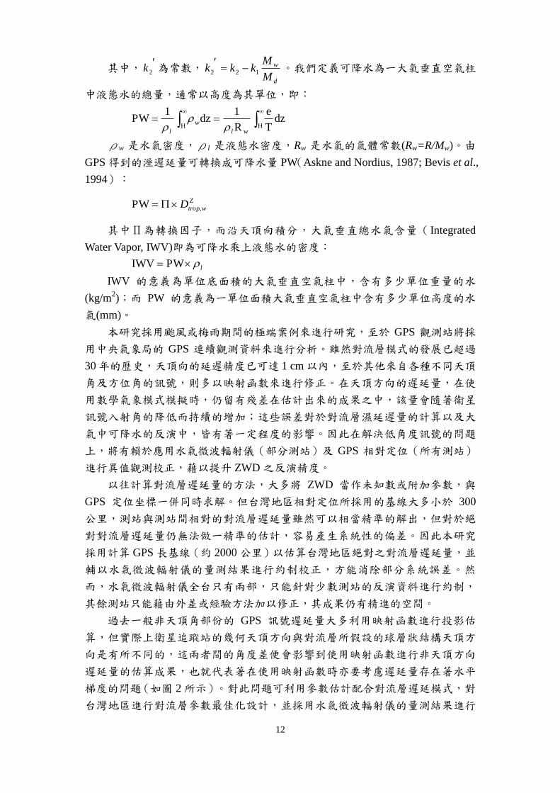
梯度的問題（如圖 2所示）。對此問題可利用參數估計配合對流層遲延模式，對

台灣地區進行對流層參數最佳化設計，並採用水氣微波輻射儀的量測結果進行

13

異質觀測約制，藉以修正此一部份之系統性誤差。

圖 2 對流層與地球幾何天頂方向示意（Hugentobler et al., 2001）

本研究除了將針對中央氣象局 GPS-ZWD 自動化計算程序進行分析，進而

解析美國專家所建立之自動化計算程序之外；也將應用地面 GPS 連續觀測資料

來進行大氣中可降水的研究，進一步提升反演的精度以消除系統誤差。就目前

的技術看來，地面 GPS 之 ZWD 計算精度已相當接近利用水氣微波輻射儀的直

接量測精度，雖然其範圍仍遠不及空中福衛三號涵蓋全球的量測資料，但卻可

提供地面的數值約制資訊，藉以提昇空中反演的精度；此外，地面 GPS 就長期

上來看，卻是一種較為經濟（地面 GPS 接收站多為現有且多功能，福衛三號所

費不貲且有其壽命限制）、近即時（觀測資料皆可近即時獲得）且全面性（台灣

本島及離島皆已覆蓋高密度的 GPS 連續接收站）的觀測方式；這將提供充足的

動機，促使我們發展以 GPS 追蹤站網近即時監測大氣的技術，透過同步匯集、

處理台灣地區 GPS 追蹤站網觀測資料，為有關單位提供快速、高空間解析力之

大氣折射資訊，進而精進短期氣象預報及長期氣候監測等工作，進而提升我國

對於氣象災害之應變能力、有效預防及減輕災害損失。

四、具體成果

1. 分析 GPS-PWV與WVR-PWV之關連性

首先要探討的是 GPS 訊號與水氣微波輻射儀是否具有關連性，本文以

WVR、GPS 觀測資料及地面氣象資料，以內政部在陽明山、北港及墾丁站所建

置的水氣微波輻射儀來分析水氣含量，由資料上所顯示的數據得知，兩者的線形

呈現一致的趨勢現象，如圖 3及 4所示。在前期北港站 GPS-PWV與WVR-PWV

的相關係數為 0.91，誤差量為-2.20 mm；而陽明山站 GPS-PWV 與 WVR-PWV

的相關係數為 0.91，誤差量為-1.45 mm，且 GPS-PWV較 WVR-PWV為低。換

句話說，假設WVR觀測的為真值，目前我們計算所得的 PWV略微低估。

14

圖 3 前期四、五、六月份北港站 GPS及WVR趨勢圖

圖 4 前期四、五、六月份陽明山站 GPS及WVR趨勢圖

15

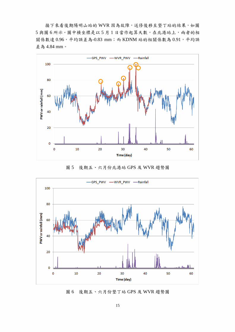
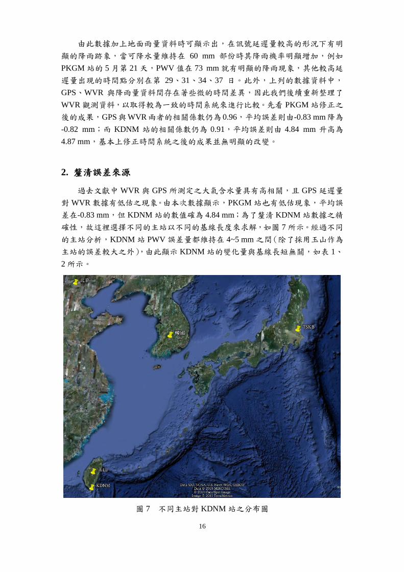
接下來看後期陽明山站的WVR因為故障，送修後移至墾丁站的結果，如圖

5與圖 6所示。圖中橫坐標是以 5月 1日當作起算天數，在北港站上，兩者的相

關係數達 0.96，平均誤差為-0.83 mm；而 KDNM站的相關係數為 0.91，平均誤

差為 4.84 mm。

圖 5 後期五、六月份北港站 GPS及WVR趨勢圖

圖 6 後期五、六月份墾丁站 GPS及WVR趨勢圖

16

由此數據加上地面雨量資料時可顯示出，在訊號延遲量較高的形況下有明

顯的降雨跡象，當可降水量維持在 60 mm 部份時其降雨機率明顯增加，例如

PKGM站的 5月第 21天，PWV值在 73 mm就有明顯的降雨現象，其他較高延

遲量出現的時間點分別在第 29、31、34、37 日。此外，上列的數據資料中，

GPS、WVR 與降雨量資料間存在著些微的時間差異，因此我們後續重新整理了

WVR觀測資料，以取得較為一致的時間系統來進行比較。先看 PKGM站修正之

後的成果，GPS與WVR兩者的相關係數仍為 0.96，平均誤差則由-0.83 mm降為

-0.82 mm；而 KDNM 站的相關係數仍為 0.91，平均誤差則由 4.84 mm 升高為

4.87 mm，基本上修正時間系統之後的成果並無明顯的改變。

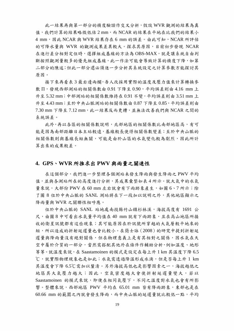
2. 釐清誤差來源

過去文獻中WVR與 GPS所測定之大氣含水量具有高相關，且 GPS延遲量

對WVR數據有低估之現象。由本次數據顯示，PKGM站也有低估現象，平均誤

差在-0.83 mm，但 KDNM站的數值確為 4.84 mm；為了釐清 KDNM站數據之精

確性，故這裡選擇不同的主站以不同的基線長度來求解，如圖 7所示。經過不同

的主站分析，KDNM站 PWV誤差量都維持在 4~5 mm之間（除了採用玉山作為

主站的誤差較大之外），由此顯示 KDNM站的變化量與基線長短無關，如表 1、

2所示。

圖 7 不同主站對 KDNM站之分布圖

17

由於 KDNM站儀器原本是放置在北部的陽明山測站上，轉移原因為陽明山

區的硫磺氣體容易造成儀器之故障，因此將儀器搬移到 KDNM站做監測；有可

能當初的更換測站並沒有做好適當的調整或校正，使偏移量的誤差值無法獲得

較佳之精度。換言之，即 KDNM站的平均誤差量與計算過程無關且無法消除，

但也證明 KDNM 站數據的真實性。本次以不同的主站求解 KDNM 站時發現，

PKGM站的相關係數還是比其他主站來得高。雖然 KDNM站的變化量與基線長

短無關，且偏移量都在 4.49~5.57 mm範圍之間，除了玉山站由於距離太接近，

大氣相關性太高無法藉由差分方式獲得準確的數據之外，其餘都還維持在高相

關；當初選擇玉山主站主要是考量該站與平地測站有相當程度的高程差，或許其

大氣環境可視為獨立不相關；但結果顯示玉山與 KDNM站基線過短導致大氣相

關性過高，因此在求解時被當成系統誤差而消除，無法獲得絕對的濕延遲量。另

外選擇關島作為主站則是基線過長，使求解之相關係數較不理想。由此推估，以

相對方式求解對流層濕延遲量，最佳解的基線距離為 1600~2400 km方能獲得較

好之精度。

表 1 採用不同主站所計算出之相關係數

採用主站基線距離 PKGM KDNM

日本 TSKB 2400 km 0.96 0.91

關島 GUAM 2700 km 0.84 0.82

玉山 YUSN 120 km 0.56 0.49

北京 BJFS 1900 km 0.91 0.90

韓國 DAEJ 1600 km 0.93 0.91

表 2 採用不同主站所計算出之偏移量（mm）

採用主站基線距離 PKGM KDNM

日本 TSKB 2400 km -0.83 4.84

關島 GUAM 2700 km 5.01 5.57

玉山 YUSN 120 km -43.51 -34.96

北京 BJFS 1900 km -1.97 4.82

韓國 DAEJ 1600 km -1.70 4.49

3. 與中央氣象局之成果進行比對

為了驗證水氣資料之真實性，接下來將本研究之計算成果，與中央氣象局委

託美國大氣研究中心（National Center for Atmospheric Research, NCAR）計算之

結果進行比對，吾人先取資料比較完整的 22 個測站，分成西部（8 站）、東部

（8站）及中央山脈（6站）三個區域，結果如表 3所示。首先，代入標準溫度

及壓力將我們計算而得的 ZWD轉換為 PWV，並與 NCAR 計算的 PWV進行比

較，結果發現以相關係數來說，西部地區的相關係數在 0.87~0.94之間，平均誤

18

差在 3.36~6.48 mm 之間；東部地區的相關係數在 0.89~0.94 之間，平均誤差在

2.50~4.54 mm 之間；中央山脈的相關係數在 0.81~0.90 之間，平均誤差在

4.81~10.09 mm之間。簡而言之，我們計算的結果與 NCAR計算的結果有高相關

性，但兩者之間存在系統誤差，在平地約為 4 mm，在山區約為 7 mm，且 NCAR

計算出來的 PWV比較小。

表 3 各站 PWV與降雨量之相關係數

雨量站 GPS站高程

(m)

標準氣象值

進行轉換之

相關係數

標準氣象值

進行轉換之

誤差(mm)

實際氣象值

進行轉換之

相關係數

實際氣象值

進行轉換之

誤差(mm)

西部地區

淡水 TANS 30 0.94 3.61 0.94 4.42

土城 TSIO 63 0.94 6.48 0.94 7.75

大肚 SALU 297 0.93 3.68 0.92 4.64

白河 TUNS 54 0.90 4.29 0.90 5.76

虎頭埤 SHWA 89 0.92 3.89 0.91 5.03

屏東 PTUN 40 0.87 4.50 0.85 5.68

岡山 CTOU 25 0.92 3.36 0.92 4.50

春日 JLUT 30 0.89 3.47 0.84 4.79

平均值 79 0.91 4.16 0.90 5.32

東部測站

福隆 FLON 41 0.94 3.10 0.94 4.03

羅東 LTUN 28 0.92 3.48 0.92 4.36

南澳 NAAO 26 0.91 2.64 0.90 3.79

富世 CHNT 38 0.92 2.50 0.90 3.48

吳全城 NDHU 57 0.91 3.92 0.89 4.72

鹿野 FENP 39 0.90 4.28 0.89 5.16

明里 DCHU 251 0.89 4.54 0.96 5.52

豐濱 LONT 203 0.91 3.63 0.90 4.37

平均值 85 0.91 3.51 0.91 4.43

中央山脈測站

大坪 WANL 370 0.70 2.21 0.93 5.00

稍來 GUKW 192 0.81 10.09 0.77 9.86

清流 DPIN 740 0.88 6.37 0.85 6.70

溪頭 SANL 1691 0.88 8.07 0.85 8.05

古夏 KASU 189 0.90 7.18 0.88 5.48

三地門 SAND 203 0.89 4.81 0.88 5.52

平均值 603 0.87 7.30 0.85 7.12

19

此一結果再與第一部分的精度驗證作交叉分析，假設WVR觀測的結果為真

值，我們計算的結果略微低估 2 mm，而 NCAR的結果在平地在比我們的結果小

4 mm，因此 NCAR與WVR結果存在 6 mm的誤差。由此可知，NCAR所評估

的可降水量與 WVR 的觀測成果差異較大。探求其原因，目前初步發現 NCAR

在進行差分相對定位時，選擇組成基線的方法為 OBS-MAX，就是讓系統自由判

斷按照觀測量較多的優先組成基線，此一作法可能會導致計算的精度下降，如第

二部分的陳述；但此一部分還必須進一步分析其系統設定之計算參數方能探討其

原因。

接下來再看表 3最右邊兩欄，吾人改採用實際的溫度及壓力值來計算轉換參

數 Π，發現西部測站的相關係數由 0.91下降至 0.90，平均誤差則由 4.16 mm上

升至 5.32 mm；中部測站的相關係數維持在 0.91不變，平均誤差則由 3.51 mm上

升至 4.43 mm；至於中央山脈測站的相關係數由 0.87下降至 0.85，平均誤差則由

7.30 mm下降至 7.12 mm，此一結果反而更糟，並無法改善我們與 NCAR之間的

系統誤差。

此外，再以各區的相關係數說明，北部地區的相關係數比南部地區高，有可

能是因為南部距離日本主站較遠，基線較長使得相關係數變差；至於中央山脈的

相關係數則與基線長短無關，可能是由於山區的水氣變化較為劇烈，因此所計

算出來的成果較差。

4. GPS、WVR所推求出 PWV與雨量之關連性

在這個部分，我們進一步整理各個測站未發生降雨與發生降雨之 PWV平均

值，並與各測站所在的高度進行分析，其成果彙整如表 4所示。就大氣中的水氣

量來說，大部份 PWV在 60 mm左右就會有下雨跡象產生，如圖 6、7所示；除

了圖 8 位於中央山脈的 SANL 測站將在下一段加以說明之外，其他地區顯示之

降雨量與WVR之關聯性相呼應。

位於中央山脈的 SANL 站地處南投縣竹山鎮杉林溪，海拔高度有 1691 公

尺，由圖 8中可看出水氣量平均值在 40 mm就有下雨跡象，且在高山地區所接

收的衛星訊號都有這些現象；其可能原因在於訊號所穿越的大氣層較平地來的

短，所以造成的折射延遲量也會比較小。在簡士詠（2008）的研究中提到折射延

遲量與降雨量沒有絕對關係，但在物理意義上是有其相對之關係，因水氣在天

空中屬於介質的一部分，當然需搭配其他外在條件作輔助分析，例如溫度、地形

等等。就溫度來說，在 Saastamoinen的模式是設定在每上升 1 km其溫度下降 6.5

℃，就實際物理現象也是如此；水氣需透過降溫形成水滴，但是否每上升 1 km

其溫度會下降 6.5℃需加以釐清。另外海拔高低也是影響因素之一，海拔越低之

地區其大氣壓力越大；因此，空氣密度越大會使折射延遲量變大，若以

Saastamoinen 的模式來說，即便在相同氣壓下，不同之溫度對水氣也會有所影

響。整體來說，西部地區 PWV 平均在 65.01 mm 皆有降雨跡象，東部也是在

60.66 mm 的範圍之內就會發生降雨，而中央山脈的延遲量就比較低一點，平均

20

值在 56.14 mm就有降雨跡象。

表 4 各站 PWV與降雨量之相關係數

編號雨量站 GPS站高程(m) 未降雨 PWV

之平均值(mm)

降雨時 PWV

之平均值(mm)

西部地區

W1 淡水 TANS 30 50.90 62.90

W2 土城 TSIO 63 53.84 67.21

W3 大肚 SALU 297 48.78 60.23

W4 北港 PKGM 42 53.35 65.84

W5 白河 TUNS 54 53.20 65.42

W6 虎頭埤 SHWA 89 52.83 64.29

W7 屏東 PTUN 40 54.89 66.87

W8 岡山 CTOU 25 52.88 66.00

W9 春日 JLUT 30 54.37 66.46

W10 墾丁 KDNM 58 52.71 64.90

平均值 73 52.78 65.01

東部測站

E1 福隆 FLON 41 50.11 61.83

E2 羅東 LTUN 28 55.61 58.44

E3 南澳 NAAO 26 52.77 61.47

E4 富世 CHNT 38 52.59 61.36

E5 吳全城 NDHU 57 53.74 60.90

E6 鹿野 FENP 39 53.08 60.19

E7 明里 DCHU 251 50.24 60.81

E8 豐濱 LONT 203 49.70 60.26

平均值 85 52.23 60.66

中央山脈

C1 大坪 WANL 370 46.52 50.72

C2 稍來 GUKW 192 52.75 63.92

C3 清流 DPIN 740 44.64 53.92

C4 溪頭 SANL 1691 34.20 41.08

C5 古夏 KASU 189 53.54 63.36

C6 三地門 SAND 203 51.85 63.82

平均值 564 47.25 56.14

21

圖 8 西部測站 JLUT站 PWV趨勢圖

圖 9 東部測站 LONT站 PWV趨勢圖

22

圖 10 中央山脈 SANL站 PWV趨勢圖

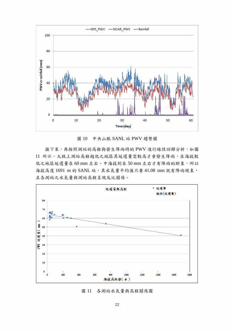
接下來，再按照測站的高程與發生降雨時的 PWV進行線性回歸分析，如圖

11 所示。大致上測站高程越低之地區其延遲量需較高才會發生降雨，在海拔較

低之地區延遲量在 60 mm左右、中海拔則在 50 mm左右才有降雨的跡象，所以

海拔高度 1691 m的 SANL站，其水氣量平均值只要 41.08 mm就有降雨現象，

且各測站之水氣量與測站高程呈現反比關係。

圖 11 各測站水氣量與高程關係圖

23

最後將 PKGM站第 21、29、31、34日等比較高延遲的部分逕行整理，釐清

在高延遲發生時，所對應累積雨量是否提前反映的現象。由圖 12中，可以發現

PKGM 站使用 WVR 所量測到的水氣量與 GPS 反演計算出的水氣量趨勢ㄧ致，

由水氣量與降雨量做比較時發現，當發生降雨時延遲量都有上升現象，由 64 mm

上升到 78 mm。由圖 13中，在 22點的時候發生了降雨，但水氣量提前一小時即

反應，大幅上升至 74 mm，從WVR與 GPS所計算出的趨勢來看，水氣量都有

明顯的上升之後才降雨。

圖 12 PKGM站第 21天延遲分量圖


24

由圖 14中也是發現大氣中的水氣含量上升後的 1~2小時即會發生降雨，以

WVR為例，在降雨前一小時水氣量即上升至 76 mm，接下來再上升到 82 mm同

時發生降雨的現象；而降雨停止之後，水氣量也跟着下降，換言之可以藉由大氣

中水氣含量的觀測來推估降雨現象。


由圖 15中得知降雨發生前一小時，水氣量由 75 mm上升到 89 mm，另一個

案例是降雨發生前一小時，水氣量從 75 mm上升到 91 mm，可知降雨現象都是

在水氣量較高時容易發生。


25

五、結論與建議

由 PKGM 站及 KDNM 站的 WVR 觀測資料，發現其水氣觀測值與 GPS 反

演計算值呈現一致的趨勢，且相關係數都在 0.9以上；此數據再加上地面雨量資

料時可顯示，在訊號延遲量較高（水氣量較高）的情況下比較容易有降雨的跡

象，一般平地測站當可降水量維持在 60 mm 時其降雨機率明顯增加。此外，

KDNM站的反演成果經由不同主站進行精度求證得知，KDNM站的變化量與基

線長短無關，其原因在儀器本身在更換測站時可能未做好適當的調整或校正，導

致誤差偏移量過大，但對數據的真實性並沒有影響，也預估出求解基線長短在

1600~2400公里的範圍內為最佳解算。

此外，假設以 WVR 的觀測值作為標準，可發現本研究 GPS 計算的水氣量

平均低估值在 2 mm，而 NCAR的計算結果則與我們的成果有 4 mm的差異；由

此可知，NCAR所評估的可降水量與WVR的觀測成果差異更大，平均來說約有

6 mm的低估。此外，測站高程越低之地區其延遲量需較高才會發生降雨，在海

拔較低之地區延遲量在 60 mm左右、中海拔則在 50 mm左右才有降雨的跡象，

所以海拔高度 1691 m的 SANL站，其水氣量平均值只要 41.08 mm就有降雨現

象，且各測站之水氣量與測站高程呈現反比關係。

六、成果的價值與貢獻

應用地面 GPS 資料來進行大氣中可降水的研究，即是利用遙測方式來反演

氣候資訊的一種方式。就目前的技術看來，其計算精度已相當接近利用水氣微

波輻射儀的直接量測精度，但其範圍遠不及空中福衛三號的量測資料；但是就

長期上來看，卻是一種較為經濟（地面GPS接收站為現有，大多用於土地測量、

板塊運動及斷層監測）、近即時（觀測資料皆可每秒傳送至控制中心）且全面性

（台灣本島及離島皆已覆蓋超過 400 站的 GPS 連續接收站）的觀測方式。本研

究藉由絕對遲延量的計算、反演大氣中可降水量、以水氣微波輻射儀進行異質

觀測約制中，可以提供相關研究人員一個相當好的學習研究經驗，藉此研究提

昇國內 GPS 氣象學及大地測量人員的素質。此外，如何導入水氣微波輻射儀資

料，分析地表氣象資料與數學氣象經驗模式對可降水反演精度之影響，這些資

訊對於往後相關的 GPS 研究來說，也是相當寶貴且有助益的。在網際網路及無

線傳輸如此發達的時空背景下，我們已經可以輕易的獲得全台灣地區的即時性

GPS 連續觀測資料，本研究因此得以近即時分析台灣地區的對流層延遲量。相

關成果除了可以應用在工程界上，未來在天氣預報、環境監測及資源災害的監

控上，或許亦可提供適當的資訊，供決策者規劃設計之用。

26

七、落實應用情形

分析地基 GPS資料處理之流程

地基 GPS-ZWD自動化計算程序流程（如圖 16所示）主要由 shell script和

perl 兩種程式語言來做整個系統程式流程控制，處理程序主要分為兩個，一個

是近即時（Near-Real Time, NRT），另一個則是全日（Daily Processing, DP）程

序。NRT每兩小時執行一次，於每日的 1:15、3:15、5:15間隔兩小時跑一次，每

次計算前 1小時至前 3小時的資料。例如：1:15跑前一天 22:00~24:00，3:15跑

當天 0:00~2:00，依此類推；目前現況由於即時資料來不及進入資料庫，故大多

只跑 1小時的資料。DP每日的 7點 30分執行，執行的每一流程結果皆有回報，

使用者可以很方便的透過回報結果來檢查出錯的流程。

而地基 GPS-ZWD自動化計算程序流程主要有五個自動化流程：

1. 取得衛星相關資料和 GPS 地基陣列資料

2. DP程序

3. 2小時 NRT程序

4. NRT狀態回報

5. 資料壓縮（Data Archiving, TBD）

今年五月開始，NCAR開始新增了每小時執行一次的流程，於 0:40、1:40、

2:40每一小時跑一次，跑前 1小時的資料。例如：0:40跑前一天 23:00~24:00，

1:40跑當天 0:00~1:00。

圖 16 地基 GPS-ZWD自動化計算程序流程

27

cwb_nrt_cron NRT(Near-Real-Time processing) 程序

NRT程序由 cwb_nrt(shell script檔)來做主要流程控制，它包含了以下七個流程：

1. 下載當日目前所有的 Rinex檔(GET RINEX FILES FOR DAY)。

2. 複製前一天 DP(Daily Processing )CRD檔(COPY NETWORK COORDINATE

FILE FROM DAILY PROCESSING)

3. 計算出內插過後的MET檔(COMPUTE MET RECORDS FROM AWS AND

MESONET STATIONS)

4. 下載衛星軌道檔案(GET IGS RAPID ORBIT PRODUCTS (SP3, ERP, SUM))

5. 下載 GIM電離層模式參數檔(GET CODE IONOSPHERE FILE)

6. 啟始 BERNESE主程式(INITIATE BPE COMMAND)

7. 繪圖並輸出至網頁(CREATE RESULT PLOTS)

如下圖所示部分流程會呼叫的 PERL檔。

28

NRT(Near Real Time processing)的子程序說明如下：

cwb_nrt_cron：呼叫 ~/bin/cwb_nrt `date -u --date "3 hour ago" '+%Y %m %d %H'`

~/bin/cwb_nrt 輸入前一天的年月日小時, 例如： 2012 02 01 12

GetRnx_rt.pl：根據/STA/igs_network裡的站下載 RINEX站資料。

GetGeonetRnxNrt.pl：同GetRnx.pl但下載 ftp://terras.gsi.go.jp/data/GPS_products/。

GetCwbRnxNrt.pl 轉換2小時 CWB T00 格式成 RINEX 格式。

GetCwbRnxNrt_rt17.pl：轉換1小時 r-17格式成 RINEX 格式。

UPPERC2：轉換檔案名稱為大寫的格式。

SmosGrd：內插 AWS和Mesonet資料。

GetOrb,pl：到 IGS網站下載 IGR軌道檔案。

GetIon.pl：到 CODE網站下載 GIM電離層模式檔案

cwb_nrt.pl：執行 Bernese BPE程序

cwb_grid_pwv.pl ：內插 PWV網格

parseStaPwv.pl：轉換 PWV檔案格式

pltStaTimeSeries.pl：繪圖並輸出至網站

ftp://terras.gsi.go.jp/data/GPS_products/

29

cwb_nrt_cron：呼叫 ~/bin/cwb_nrt `date -u --date "3 hour ago" '+%Y %m %d %H'`

~/bin/cwb_nrt 輸入前一天的年月日小時, 例如： 2012 02 01 12

~/John/cwb_nrt是一個 Shell script檔，所有 NRT(Near Real Time processing)透過

它來呼叫所有子程序，以下為 cwb_nr程式碼(藍色底為程式碼)說明：

設定 Bernese Campaign 路徑和指定 PCF(procedure control file)檔。

設定輸入的日期轉為 GPS常用的日期格式，方便 Bernese呼叫使用。

cwb_nrt_cron

cwb_nrt

CAMP_PATH=$P #設定 Bernese Campaign 路徑$P 是指/pub/john/GPSDATD

CAMPAIGN=CWB_NRT #指定 Campaign 名稱

PCF=CWB_NRT #指定 PCF(procedure control file)檔名稱

CAMP_PATH_POST_PROC=$P

CAMPAIGN_POST_PROC=CWB_DP #找 Weekly coordinate solutions (CRD)檔的路

徑用

yr=$1 #獲得輸入的四個參數年月日小時

mo=$2

day=$3

hour=$4

y2=ècho $yr | cut -c3-4` #傳換為 GPS 的日期格式

gweek=`ymd2gps $yr $mo $day| awk '{print $1}'`

gweekm1=`ymd2gps $yr $mo $day| awk '{print $1-1}'`

gday=`ymd2gps $yr $mo $day| awk '{print $2}'`

dom=ècho $day | awk '{printf("%02i",$1)}'`

day=`ymd2doy $yr $mo $day |awk '{printf("%03i",$2)}'`

mjd=`doy2mjd ${yr} ${day} | awk '{printf("%05d",$1)}'`

S=`GetCharSes.pl $hour` #呼叫 GetCahrSes.pl 把小時的整數轉為英文字母，方便程式使用

30

在這裡一共呼叫 GetRnx_rt.pl、GetCwbRnxNrt.pl、GetGeonetRnxNrt.pl和

GetCwbRnxNrt_rt17.pl四個 Perl的程式檔，以下為這四個程式的說明：

程式執行流程概述：

移至 /pub/john/GPSDATA / CWB_NRT /RAW目錄

1. 下載鄰近台灣的 IGS追蹤站(紀錄於對應的/SAT/igs_network檔案中)

的 RINEX資料，並根據 igs_network列表的 IGS追蹤站的 ftp站下載

RINEX資料。

2. 因為每一 IGS追蹤站的儀器、天線盤、天線高度和檔案的格式都不進

相同，因此需要先呼叫 UNAVCO聯盟提供的 teqc程式做 RINEX檔頭

的轉換符合 Bernese的輸入格式，才能讓 Bernese主程式順利的運作。

Input： igs_network 年日時

Output：修正過後的 RINEX data(副檔名為 .xxo ，xx為年)

#下載所有必需的 RINEX 檔。

echo " "

echo "RETRIEVING RINEX FILES"

echo " "

#切換到/pub/john/GPSDATDATA/ CWB_NRT/RAW 目錄下

cd ${CAMP_PATH}/${CAMPAIGN}/RAW

# Get data from IGS network

gunzip *${day}*.gz

GetRnx_rt.pl ../STA/igs_network ${yr} ${day} ${hour} 2> /dev/null

GetCwbRnxNrt.pl ../STA/cwb_network ${yr} ${day} ${hour} 2> /dev/null

GetGeonetRnxNrt.pl ../STA/geonet_network ${yr} ${day} ${hour} 2> /dev/null

GetCwbRnxNrt_rt17.pl ../STA/cwb_network ${yr} ${day} ${hour} 2> /dev/null

$X/EXE/UPPERC2 ${day}?.${y2}?

GetRnx_rt.pl

31


移至 /pub/john/GPSDATA / CWB_NRT /RAW目錄

執行的流程大致同 getRnx_rt.pl，只是下載的 GPS資料網為日本的 GEONET GPS

網路，並根據 SAT/geonet_network檔案裡的所列的站下載所需的 GPS檔案。

Input： geonet_network 年日時


Input igs_network Year Day Hour

Read in IGS stations

list

Check one IGS station parameters

wget Rinex file

Uncompress Rinex

file

Correct Rinex file head

(Call teqc)

Next IGS station ?

GetRnx_rt.pl

GetGeonetRnxNrt.pl

32


移至 /pub/john/GPSDATA / CWB_DP /RAW目錄

執行的流程大致同 getRnx_rt.pl，但省去的下載 Rinex檔的程式碼，因為氣象局

內部的 GPS t00資料是自動上傳至氣象局內部的磁碟陣列，所以不需要下載。

1. 氣象局的 GPS資料位於/ops/cwb/t00，因為 t00資料並不是 Rinex檔的格式，

所以需要呼叫 trimble提供的 runpkr00程式把 t00檔轉至 Rinex檔格式。

Input geonet_network Year Day Hour

Read in geonet stations list

Check one station parameters

wget Rinex file

Uncompress Rinex

file


(Call teqc)

Next station ?

GetGeonetRnxNrt.pl

GetCwbRnxNrt_rt17.pl

33

Input： cwb_network 年日時



移至 /pub/john/GPSDATA / CWB_DP /RAW目錄

執行的流程大致同 getRnx_rt.pl，但省去的下載 Rinex檔的程式碼，因為氣象局

內部的 GPS rt17資料是自動上傳至氣象局內部的磁碟陣列，所以不需要下載。

2. 氣象局的 GPS資料位於/ops/cwb/t00，因為 rt17資料並不是 Rinex檔的格式，

Input cwb_network Year Day Hour

Read in cwb_network

stations list

Check one station parameters

Convert from T00 to Rinex

File (call runpkr00)


(Call teqc)

Next station ?

GetCwbRnxNrt.pl

GetCwbRnxNrt_rt17.pl

34

所以需要呼叫 UNAVCO聯盟提供的 teqc程式把 rt17檔轉至 Rinex檔格式並

修正 Rinex檔頭資訊。

Input： cwb_network 年日時


在 DP(Diary Processing)的程序會依據 GPS week的第一天輸出一 CRD檔，紀錄

每一 GPS接收站的位置(A-priori Coordinate Information)當成參考值，沒有這

個檔案，後續的 Bernese主程式會顯示錯誤，結果將會跑不出來。

35

##########################################################

# GET COORDINATE FILE FROM LAST WEEK DAILY SOLUTION

##########################################################

echo " "

echo "RESOLVING APRIORI COORDINATE FILE "

echo " "

#切換到/pub/john/GPSDATDATA/ CWB_NRT/STA 目錄下

cd ${CAMP_PATH}/${CAMPAIGN}/STA

if [ -f NET${gweekm1}7.CRD ] #找到了 CRD 檔

then

echo "COORDINATE FILE ALREADY EXISTS "

HAVE_CRD=0

#如果在 STA 目錄下沒找到，就去 CWB_DP 目錄下尋找

elif [ -f

${CAMP_PATH_POST_PROC}/${CAMPAIGN_POST_PROC}/STA/NET${gweek

m1}7.CRD ]

then

echo "COORDINATE FILE ALREADY EXISTS " #找到了 CRD 檔

cp

${CAMP_PATH_POST_PROC}/${CAMPAIGN_POST_PROC}/STA/NET${gweek

m1}7.CRD .

HAVE_CRD=0

else

echo "WE HAVE TROUBLE "

echo "NO NETWORK COORDINATE FILE FOUND "

HAVE_CRD=-1 #未找到 CRD 檔，並輸出錯誤訊息

fi

36

以下 cwb_nr部分程式碼主要工作是利用氣象局的資料內插出每一GPS接收站上

方的大氣資料。

##########################################################

# Interpolate surface observations to GPS Station Locations

##########################################################

echo " "

echo "INTERPOLATING AWS AND MESONET RECORDS"

echo " "

#切換到/pub/john/GPSDATDATA/ CWB_NRT/ATM/SmosGrd 目錄

cd ${CAMP_PATH}/${CAMPAIGN}/ATM/SmosGrd

cp /ops/aws/rsdf${y2}${mo}${dom}??.dat . #複製最新的 aws 資料至目錄下

cp /ops/mesonet/rsnf${y2}${mo}${dom}??.dat . #複製最新的 mesonet 資料

#執行內插程式 SmosGrd.pl

SmosGrd.pl --crdfil

${CAMP_PATH}/${CAMPAIGN}/STA/NET${gweekm1}7.CRD \

--year ${yr} --day ${day} \

rsdf${y2}${mo}${dom}??.dat rsnf${y2}${mo}${dom}??.dat

#刪除目錄下的 aws 和 mesonet 資料

rm rsdf${y2}${mo}${dom}??.dat rsnf${y2}${mo}${dom}??.dat

#將每 GPS 站上方內插出的大氣資料(.MET 檔)移到/pub/john/GPSDATDATA/

CWB_NRT/ATM/目錄

for fil in ????${day}0.MET

do

if [ -s $fil ]

then

mv ${fil} ../.

fi

done

37

以下是內插程式 SmosGrd.pl的說明：


整個系統使用氣象局兩個主要的資料群，一是氣象局 GPS地面觀測站資料，

包含兩個小時的 t00格式資料和一個小時 rt17的 Rinex資料，另一是地面氣象觀

測資料(automated weather system (AWS) and mesonet networks)包含溫度、壓力、

風向、風力等，主要由 automatic meteorological data processing system (AMDP)系

統運作管理。以下為 SmosGrd.pl程式所需要輸入的資料說明：

AWS data：

每個文件包括各站的氣壓，溫度，風向和相應的高度，緯度，經度和觀測時

間。文件名稱是 rsdfyyMMDDhhmm.dat格式，檔案位於/pub/aws目錄下，目前

每小時一筆檔案。

Mesonet data：

每個文件包括各站氣壓，溫度，露點溫度(dew-point)，風向和相應的高度，

經度，緯度和觀測時間。文件名稱是 rsnfyyMMDDhhmm.dat格式，檔案位於

/pub/mesonet目錄下，目前每小時一筆檔案。

A-priori Coordinate Information：

根據 IGS追踪站所發佈座標的包括 ITRF和 IGS參考坐標可作為一參考的資

訊，亦是 bernese運算的重要參考數據，否則無法算出較精確的定位點。在本程

式中是用來獲取每一 GPS接收儀的位置，再內插出 GPS站上方的天氣資訊，文

件名稱是 APR_MMyy.CRD.dat格式，檔案位於$P/CWB_DP/STA目錄下。

因為計算 ZTD轉換為 PWV時需要當地 GPS站上方的溫度和壓力值，但不是

每一個 GPS站都有這些相對應的觀測儀器，因此透過氣象局的 AWS和Mesonet

的資料網內插出位於 APR_MMyy.CRD中所有 GPS站上方的溫度和壓力值。在

SmosGrd.pl程式中，在內插前需先進行網格化(網格精度為 0.1(經緯度))，而為了

消除資料間的不一致性，本程式採用 GMT軟體所提供的 blockmedian演算法作

前處理每單一網格內的資料，然後呼叫 GMT的 Surface程式(adjustable tension

continuous curvature surface gridding algorithm, Smith, W. H. F, and P. Wessel, 1990)

指令內插出所有網格的值(tension factor T = 0.1)，有了網格內的所有內插值後，

再根據 APR_MMyy.CRD裡的找出所有 GPS站上方的溫度和壓力值，並輸出至

MET檔。

SmosGrD.pl

38

首先移至 /pub/john/GPSDATA / CWB_NRT /ATM/SmosGrd目錄，將

/ops/aws/rsdf${y2}${mo}${dom}.dat和/ops/mesonet/rsnf${y2}${mo}${dom}.dat的

資料複製到/pub/john/GPSDATA / CWB_NRT /ATM/SmosGrd目錄中。

Input： APR_${mo}${y2}.CRD --year ${1} --day ${day}

rsdf${y2}${mo}${dom}??.dat rsnf${y2}${mo}${dom}??.dat

Output：所有 GPS站的MET檔於$P/CWB_NRT/ATM中。

此程式需四個 perl的模組 File_IO、Geo_Subs、Time_Subs和 Getopt::Long，

File_IO、Geo_Subs、Time_Subs三個 PM檔位位於~john/bin目錄下，Getopt::Long

可以透過 CPAN安裝即可。

以下 cwb_nr部分程式碼，主要工作是下載 GPS廣播星曆，如有重複則更新，沒

有更新到的話先用舊的。

39

##########################################################

# GET ORBIT FILES

##########################################################

echo " "

echo "RETRIEVING ORBIT FILES"

echo " "

#切換到/pub/john/GPSDATDATA/ CWB_NRT/ORB 目錄

cd ${CAMP_PATH}/${CAMPAIGN}/ORB

#下載最新版的星曆前，先把檔名改為_OLD

if [ -f IGU${gweek}${gday}.SP3 ] && [ -f IGU${gweek}${gday}.IEP ]

then

mv IGU${gweek}${gday}.SP3 IGU${gweek}${gday}_OLD.SP3

mv IGU${gweek}${gday}.IEP IGU${gweek}${gday}_OLD.IEP

fi

#下載最新的廣播星曆

GetOrb.pl igu ${yr} ${day}

$X/EXE/UPPERC2 igu

# 檢查是否是最新的廣播星曆，如果沒有就先用前一個最新來用

if [ -f IGU${gweek}${gday}_18.SP3 ] && [ -f IGU${gweek}${gday}_18.ERP ]

then

cp IGU${gweek}${gday}_18.SP3 IGU${gweek}${gday}.SP3

cp IGU${gweek}${gday}_18.ERP IGU${gweek}${gday}.IEP

elif [ -f IGU${gweek}${gday}_12.SP3 ] && [ -f

IGU${gweek}${gday}_12.ERP ]

then



40

以下是 GetOrb.pl的說明：

移至 /pub/john/GPSDATA / CWB_NRT /ORB目錄


本程式至 IGS CNETER(如表)下載 IGS衛星軌道檔(IGS orbit file)和地球自轉資

訊檔(earth rotation files)，這兩個檔案用來定義整體參考座標(global reference



then





then



#如果都沒有下載到星曆只好先用上一次下載(_OLD 檔)的

elif [ -f IGU${gweek}${gday}_OLD.SP3 ] && [ -f

IGU${gweek}${gday}_OLD.ERP ]

then

cp IGU${gweek}${gday}_OLD.SP3 IGU${gweek}${gday}.SP3

cp IGU${gweek}${gday}_OLD.IEP IGU${gweek}${gday}.IEP

fi

if [ -f IGU${gweek}${gday}.SP3 ] && [ -f IGU${gweek}${gday}.IEP ]

then

HAVE_ORB=0 #有廣播星曆

echo "ORBIT FILE: " `ls -lrt IGU${gweek}${gday}.SP3`

echo "ERP FILE : " `ls -lrt IGU${gweek}${gday}.IEP`

else

HAVE_ORB=1 #通知系統沒有廣播星曆

fi GetOrb.pl

41

frame)。檔案下載完後置放於/pub/john/GPSDATA / CWB_NRT /ORB目錄裡。

Archive Center Path

CDDIS ftp://cddis.gsfc.nasa.gov/gps/products/WWWW/

SOPAC ftp://garner.ucsd.edu/pub/products/WWWW/

IGN ftp://igs.ensg.ign.fr/pub/igs/products/WWWW/

IGSCB ftp://igscb.jpl.nasa.gov/pub/product/WWWW/

Input： Year Day

Output：附檔名為.sp3 和.sum的檔案

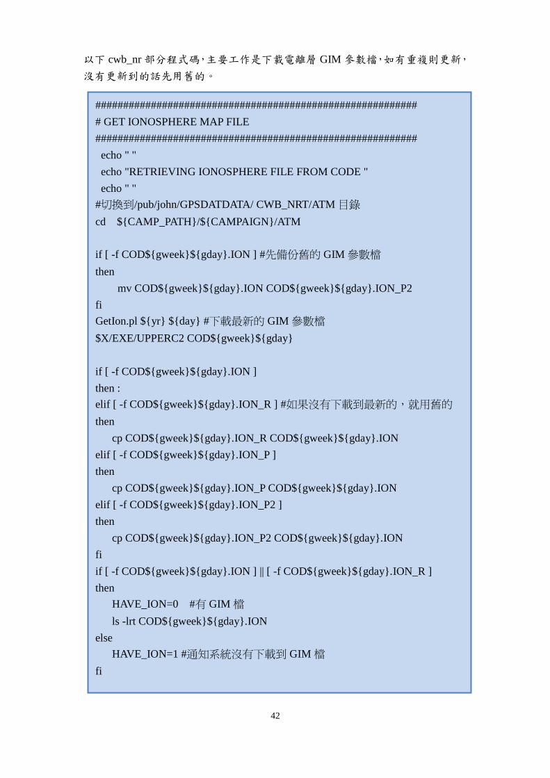
42

以下 cwb_nr部分程式碼，主要工作是下載電離層 GIM參數檔，如有重複則更新，

沒有更新到的話先用舊的。

##########################################################

# GET IONOSPHERE MAP FILE

##########################################################

echo " "

echo "RETRIEVING IONOSPHERE FILE FROM CODE "

echo " "

#切換到/pub/john/GPSDATDATA/ CWB_NRT/ATM 目錄

cd ${CAMP_PATH}/${CAMPAIGN}/ATM

if [ -f COD${gweek}${gday}.ION ] #先備份舊的 GIM 參數檔

then

mv COD${gweek}${gday}.ION COD${gweek}${gday}.ION_P2

fi

GetIon.pl ${yr} ${day} #下載最新的 GIM 參數檔

$X/EXE/UPPERC2 COD${gweek}${gday}

if [ -f COD${gweek}${gday}.ION ]

then :

elif [ -f COD${gweek}${gday}.ION_R ] #如果沒有下載到最新的，就用舊的

then

cp COD${gweek}${gday}.ION_R COD${gweek}${gday}.ION

elif [ -f COD${gweek}${gday}.ION_P ]

then

cp COD${gweek}${gday}.ION_P COD${gweek}${gday}.ION

elif [ -f COD${gweek}${gday}.ION_P2 ]

then

cp COD${gweek}${gday}.ION_P2 COD${gweek}${gday}.ION

fi

if [ -f COD${gweek}${gday}.ION ] || [ -f COD${gweek}${gday}.ION_R ]

then

HAVE_ION=0 #有 GIM 檔

ls -lrt COD${gweek}${gday}.ION

else

HAVE_ION=1 #通知系統沒有下載到 GIM 檔

fi

43

以下是 GetIon.pl的說明：

移至 /pub/john/GPSDATA / CWB_NRT /ATM目錄


本程式至 ftp://ftp.unibe.ch/aiub/CODE/下載 GIM參數檔(CODE Global

Ionosphere Model (GIM) Files)，GIM是一電離層模式，在 Bernese軟體中的

CWB_NRT.PCF 和 CWB_PWV.PCF會使用到，它利用 QIF(Quasi-Ionosphere Free

(QIF) method)方法抵銷電離層延遲(Ionospheric Delay)的影響，但還是有剩餘的

residual ionospheric error造成未定解(ambiguities)，在 Bernese軟體中則透過 GIM

電離層模式來剔除掉。檔案下載完後置放於/pub/john/GPSDATA / CWB_NRT

/ATM目錄裡

Input： Year Day

OutPut：附檔名為.ION的檔案

GetIon.pl

ftp://ftp.unibe.ch/aiub/CODE/

44

以下 cwb_nr部分程式碼，主要工作是呼叫 Bernese執行主要的計算工作。


透過程式 cwb_nrt.pl 呼叫 Bernese軟體執行，因為 Bernse軟體的主程式也是透

過 perl語言執行，因此本程式主要工作就是設定 NRT(Near Real Time processing)

的參數(PCF檔)然後呼叫 Bernese主體執行，運算結果輸出 PWV檔至

/pub/john/GPSDATDATA/ CWB_NRT/ATM裡。

如上圖所示，我們可以得知在執行 cwb_nrt.pl之前的所有程式，都是執行綠

色區塊 BPE (Bernse Processing Engine)前的準備工作(藍色方塊部分)，當所有的

藍色區塊的資料都順利正確產生後，呼叫 BPE才會計算出黃色區塊的資料，BPE

根據 CWB_NRT.PCF(如下表所示)裡的設計來呼叫 Bernese所有子程序來執行：

# Initiate BPE Command

#執行/home/john/BERN50/GPSUSER/SCRIPT 裡的 cwb_nrt.pl 檔

$U/SCRIPT/cwb_nrt.pl ${yr} ${day}${S}

cwb_nrt.pl

45

# Procedure Control File (PCF)

# All comment lines start with a #

# Comments:

#

#

PID SCRIPT OPT_DIR CAMPAIGN CPU P WAIT FOR....

3** 8******* 8******* 8******* 8******* 1 3** 3** 3** 3** 3** 3** 3** 3** 3** 3**

#

# Translate Pole Files in ORB/ Directory

#

003 POLUPD NRT_ORB ANY 0

#

# Generate Standard Orbits and Sat. Clocks

#

010 PRETAB NRT_ORB ANY 0 003

011 ORBGEN NRT_ORB ANY 0 010

#

# Zero Difference File Processing (RXOBV3 and CODSPP)

#

#018 PREP_RNX ZDP any 002

019 RNXGRA NRT_ZDP ANY 0 011

020 RXOBV3 NRT_ZDP ANY 0 019

021 CODSPP NRT_ZDP ANY 0 020 011

022 CODXTR NRT_ZDP ANY 0 021

#

# Single Difference Creation (SNGDIF)

#

030 SNGDIF NRT_MAXO ANY 0 022

#

# Clean Single Differences of Cycle Slips (MAUPRP)

#

040 MAUPRP NRTCLEAN ANY 0 030

041 MPRXTR NRTCLEAN ANY 0 040

042 GPSEDTAP NRTCLEAN ANY 0 041

043 GPSEDT_P NRTCLEAN ANY 0 042

044 GPSRMSCK NRT_CHK ANY 0 043

#

# Compute network solution based on amb free basline solutions

#

045 ADDNEQ2 NRT_CHK ANY 1 044

046 GPSXTR NRT_CHK ANY 1 045

#

# Resolve Ambiguities Baseline Wise (GPSEST)

#

050 GPSQIFAP NRT_QIF ANY 0 046

051 GPSQIF_P NRT_QIF ANY 0 050

052 GPSXTR NRT_QIF ANY 0 051

#

# Compute Troposphere Solution

#

060 GPSEST NRT_TRP ANY 0 052

061 STK_NEQ NRT_TRP ANY 0 060

062 TRO_2PW NO_OPT ANY 0 060

063 TRO_2PW NO_OPT ANY 0 061

#

# Clean up and create summary files

#

090 SES_CLN NO_OPT ANY 0 061

091 NRT_SUM NO_OPT ANY 0 090

#

#

999 DUMMY NO_OPT ANY 1 091

#

# additional parameters required for PID's

#

PID USER PASSWORD PARAM1 PARAM2 PARAM3 PARAM4 PARAM5 PARAM6

PARAM7 PARAM8 PARAM9

3** 12********** 8******* 8******* 8******* 8******* 8******* 8******* 8******* 8******* 8*******

46

8*******

#

042 $042

043 PARALLEL $042

044 NEXTJOB 030

#

#050 $050

#051 PARALLEL $050

#

050 SKIP

051 SKIP

052 SKIP

#

062 TD_ suomiday Bv95 CWB_NRT SUOMI LOCAL

063 TRP suomiday Bv95 CWB_NRT SUOMI LOCAL

#

091 CWB_NRT

#

#

VARIABLE DESCRIPTION DEFAULT

8******* 40************************************** 16**************

V_O TWO CHARACTER PREFIX FOR ORBITS IGU

V_PLUS VARIABLE FOR NUMBER OF FORWARD SES 0

V_MINUS VARIABLE FOR NUMBER OF PREV SESS -6

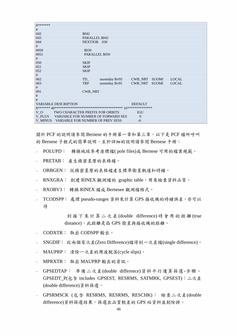
關於 PCF的說明請參閱 Bernese的手冊第一章和第三章，以下是 PCF檔所呼叫

的 Bernese子程式的簡單說明，至於詳細的說明請參閱 Bernese手冊：

– POLUPD：轉換地球參考座標檔( pole files)成 Bernese可用的檔案規範。

– PRETAB：產生精密星曆的表格檔。

– ORBGEN：從精密星曆的表格檔產生標準衛星軌道和時鐘。

– RNXGRA：創建 RINEX觀測檔的 graphic table，用來檢查資料品質。

– RXOBV3：轉換 RINEX檔成 Bernesee觀測檔格式。

– TCODSPP：處理 pseudo-ranges資料來計算 GPS接收機的時鐘誤差，亦可以

得

到接下來計算二次差 (double difference)時會用的距離 (true

distance)，此距離是指 GPS衛星與接收機的距離。

– CODXTR：取出 CODSPP輸出。

– SNGDIF：從兩個零次差(Zero Difference)檔得到一次差檔(single difference)。

– MAUPRP：清除一次差的周波脫落(cycle slips)。

– MPRXTR：取出MAUPRP輸出的資訊。

– GPSEDTAP：準備二次差 (double difference)資料平行運算篩選 -步驟。

GPSEDT_P(包含 includes GPSEST, RESRMS, SATMRK, GPSEST)：二次差

(double difference)資料篩選。

– GPSRMSCK (包含 RESRMS, RESRMS, RESCHK)：檢查二次差(double

difference)資料篩選結果，篩選出品質較差的 GPS站資料並剔除掉。

47

– ADDNEQ2：堆疊正規方程式(normal equations)並檢查接收站是否有錯誤的

基線解，計算所有基線(baselines)解(含網路解和單一基線解)的時候會使用到

ADDNEQ2。

– GPSXTR：取出 ADDNEQ2的輸出檔資訊。

– GPSQIFAP (含 BASLST)：準備平行(parallel)運算 QIF 未定解(ambiguity

resolution)程序，QIF只算 GPSXTR 輸出的基線(baselines)。

– GPSQIF_P (含 GPSEST)：計算網路解(network solution)

– GPSXTR：取出 GPSEST的輸出檔資訊

– GPSEST：估算 GPS載波相位觀測資料的相關參數。

– TK_NEQ (含 ADDNEQ2)：估算每兩小時的ZTD，並且整併到12小時的TRP。

– TRO_2PW：轉換 ZTD檔(TRP格式)成 PW檔。

– TRO_2PW：同上

– SES_CLN：刪除相關不在需要的檔案。

– SES_SUM：輸出 NRT處理程序的摘要檔(CWByyssss.PRC)。

在 Bernese執行的當中，BPE Server會即時更新最新的狀態到 RUNBPE.OUT，

如果有錯誤，使用者可以到/CWB_NRT/BPE下找到 RUNBPE.OUT的錯誤回報，

檢查問題並解決它。

Time Sess PID Script Option Status

--------------------------------------------------------------------------------

11-Jun-2008 01:28:53 162O YR:2008 CWB_NRT : Server started at 44231 11-Jun-2008 01:28:57 162O 003_000 POLUPD NRT_ORB : Client started

11-Jun-2008 01:28:57 162O 003_000 POLUPD NRT_ORB : Script started

11-Jun-2008 01:28:58 162O 003_000 POLUPD NRT_ORB : Script finished OK 11-Jun-2008 01:28:58 162O 010_000 PRETAB NRT_ORB : Client started

11-Jun-2008 01:28:58 162O 010_000 PRETAB NRT_ORB : Script started

11-Jun-2008 01:28:59 162O 010_000 PRETAB NRT_ORB : Script finished OK 11-Jun-2008 01:28:59 162O 011_000 ORBGEN NRT_ORB : Client started

11-Jun-2008 01:28:59 162O 011_000 ORBGEN NRT_ORB : Script started

11-Jun-2008 01:29:03 162O 011_000 ORBGEN NRT_ORB : Script finished OK 11-Jun-2008 01:29:03 162O 019_000 RNXGRA NRT_ZDP : Client started

11-Jun-2008 01:29:03 162O 019_000 RNXGRA NRT_ZDP : Script started

11-Jun-2008 01:29:06 162O 019_000 RNXGRA NRT_ZDP : Script finished OK 11-Jun-2008 01:29:06 162O 020_000 RXOBV3 NRT_ZDP : Client started

11-Jun-2008 01:29:06 162O 020_000 RXOBV3 NRT_ZDP : Script started

11-Jun-2008 01:29:12 162O 020_000 RXOBV3 NRT_ZDP : Script finished OK 11-Jun-2008 01:29:12 162O 021_000 CODSPP NRT_ZDP : Client started

11-Jun-2008 01:29:12 162O 021_000 CODSPP NRT_ZDP : Script started

11-Jun-2008 01:29:39 162O 021_000 CODSPP NRT_ZDP : Script finished OK 11-Jun-2008 01:29:39 162O 022_000 CODXTR NRT_ZDP : Client started

RUNBPE.OUT檔

RUNBPE.OUT檔只是簡單的說明每一個 Bernese子程序的運算結果，在 PCF檔

裡每個子程序都有設定一 PID(process ID)號碼，每個 PID程序都會輸出相對應的

PRT檔(位於$P/CWB_NRT/BPE)，也就是說明每 PID程序的摘要檔，如下表所示：

48

PROTOCOL FILE FOR BPE SCRIPT

----------------------------

Campaign : ${P}/CWB_NRT Year : 08

Session : 162O

PCF name : CWB_NRT.PCF Script name : TRO_2PW

Path to executables: ${XG}

Option directory : NO_OPT Process ID : 063

Sub-process ID : 000

Server host : taccop4g.cwb.gov.tw Remote host : taccop4g.cwb.gov.tw

CPU name : localhost

Path to work area : /home/john/GPSTEMP/BPE_CWB_NRT_44231_08_162O_063_000 User name : john

Date Time Run time Pgm.time Sta Program Message ----------------------------------------------------------------------------

11-JUN-2008 01:37:29 00:00:00 MSG RUNBPE.pm SCRIPT STARTED

11-JUN-2008 01:37:29 00:00:00 MSG RUNBPE.pm SCRIPT STARTED 11-JUN-2008 01:37:32 00:00:03 MSG RUNBPE.pm SCRIPT ENDED

----------------------------------------------------------------------------

當DP和NRT的Bernese運算的成功執行完後，除了上述的摘要檔(RUNBPE.OUT

與 PRT檔)外，剩下就是運算結果的相關檔案，以下是這些結果檔的相關說明：

Daily coordinate solutions (CRD)：日 CRD檔

每當 DP的程序執行完就會有 Daily coordinate CRD的座標檔被產生出來，由

CWB_PWV.PCF檔中 060 PID程序(Compute Network Geodetic Solution)跑完輸出

至$P/CWB_DP/STA目錄中，每一天產生一個檔，檔案格式為 NETwwwwd.CRD，

wwww指的是 GPS week，而 d是指 GPS week當中的第幾天，如果是 GPS week

的第三天，d則是 3，NETwwwwd.CRD是由 NETwwwwd.NQ0檔(Daily Normal

Equation files)演算出來的，取名”NET”是因為它是由所有 GPS站網路所算出的

解，另一類的 CRD檔則是則是由每一 GPS站的基線(baseline)所算出來的，因此

取名為”BSL”，檔案格式為 BSLwwwwd.CRD，同樣的，它也是由 BSLwwwwd.NQ0

所演算來的。

Daily Normal Equation files (NQ0)：日法線檔

NQ0檔是 DP(Daily Processing)的法線方程式檔，檔案位於$P/CWB_DP/SOL，格

式為 NETwwwwd.NQ0，wwww指的是 GPS week，而 d是指 GPS week當中的第

幾天，如果是 GPS week的第一天，d則是 1，由 CWB_PWV.PCF檔中 060 PID

程序(Compute Network Geodetic Solution)輸出的，之後 ADDNEQ2將會利用 NQ0

檔產生出 weekly coordinate solutions CRD檔。其他的法線檔，包含計算單一基

線的 BSLwwwwd.NQ0檔是 NRT的程序產生出來的，而 TD_wwwwd.NQ檔則是

由 DP程序產生出來的。

49

Weekly coordinate solutions (CRD)：周 CRD檔

在 DP程序中的 PID 070(ADDNEQ2)會將之前計算出的整日 CRD檔產生周 CRD

檔(Weekly coordinate solutions (CRD))，檔案位於$P/CWB_DP/STA目錄裡，格式

為 NETwwww7.CRD，wwww指的是 GPS week，每 GPS week中的第一天，DP

程序會被指定要產出一周 CRD檔，所以這代表前七天的對流層的運算已經成功

的分析完成，所以周 CRD檔將會用來獲得下一周的所有 GPS站的先期座標

(a-priori coordinates)(內插氣象局大氣資料會使用到)，以及協助 DP程序中的 PID

075(GPSEST)和 PID 076(ADDNEQ2)對流層資料解算，例如在 GPS week 1450周

當中七天的座標解將會用來計算 GPS week 1451周的對流層結果。

Weekly SINEX files (SNX)：周 SNX檔

SINEX(Solution Independent Exchange)檔記錄了一周的GPS網座標的計算結果和

它們的諧方差(covariance)，格式為NETwwwwd.SNX，命名方式與Daily coordinate

solutions (CRD)相同，檔案位於$P/CWB_DP/SOL中，每天產生一次，SINEX檔

的用途很多，包含數周的座標解算到單一基站的解算都會用到它，例如每產生一

SINEX檔可用來協助獲得當週的法線方程式(normal equation file)和座標解。

Zenith Troposphere Estimates：天頂對流層估算

天頂對流層的計算結果包含兩類資料，一是 ZTD(zenith troposphere delay)和

PW(precipitable water)兩種，ZTD包含乾遲延(hydrostatic Zenith)和濕遲延項(wet

Zenith)，因此需要大氣總氣壓(surface pressure)的測量資料才能隔離出濕遲延項，

而 PW則由濕遲延項推導出來的

(1) ZTD資料把所有 GPS站的天頂延遲量整合到一個檔案裡，格式是

TD_yySSSS.TRP，yy代表年，SSSS代表 Bernese PCF的 session數字，檔案位

於$P/CWB_DP/ATM，每一檔案包含先期的天頂延遲(a-priori zenith delay)，天

頂延遲的修正量，先期和天頂延遲修正量的總和，和錯誤估計等，詳細的說

明請參考 Bernse manual 22.9章節。 TRP檔範例如下表所示：

NETWORK TROPOSPHERE SOLUTION: 122290 19-SEP-12 12:44

-------------------------------------------------------------------------------------------------------------------------------------

A PRIORI MODEL: -15 MAPPING FUNCTION: 4 GRADIENT MODEL: 0 MIN. ELEVATION: 5 TABULAR INTERVAL: 1800 / 0

STATION NAME FLG YYYY MM DD HH MM SS MOD_U CORR_U SIGMA_U TOTAL_U AKND P 2012 08 16 00 00 00 2.2895 0.39128 0.00292 2.68080

AKND P 2012 08 16 00 30 00 2.2895 0.40764 0.00193 2.69717

AKND P 2012 08 16 01 00 00 2.2895 0.37794 0.00159 2.66746 AKND P 2012 08 16 01 30 00 2.2895 0.36815 0.00151 2.65767

AKND P 2012 08 16 02 00 00 2.2895 0.36600 0.00265 2.65552

50

NRT程序的 ZTD檔案格式是 TD_yySSSS.TRP，資料包含 2小時到 14小時

的範圍，間距為 2小時，而 DP程序的 ZTD檔案格式是 TD_yySSS0.TRP，資料

共有 26小時的數據，間距一樣是 2小時。

另外 troposphere SINEX檔一樣也會一起被產生出來，副檔名為 TRO檔，內容是

一樣的，只是資料格式不同而已。

(2) PW資料把所有 GPS站的天頂濕延遲量整合到一個檔案裡，在 NRT程序中檔

案格式是 CWB_NRTTD_yySSSS.PWV，是從天頂延遲量 TD_yySSSS.TRP推導

而來，檔案位於$P/CWB_NRT/ATM，相對的，如果是 DP程序的話，PW檔

案格式是 CWB_DPTD_yySSS0.PWV，是從 TD_yySSS0.TRP推導而來，檔案

位於$P/CWB_DP/ATM目錄裡。

PW檔案格式的說明如下

– Site： GPS站名。

– PWVmidTim：兩個 epochs 時間的中間內插值，如果是0015，代表他是0000

和0030的內插中間值。

– Duration：兩個 epochs之間的間格式間 (Unit: minutes)

– PW：估算的可降水量(Precipitable water vapor estimates) (Unit: mm)

– FMerr：可降水量的錯誤量 (Formal error)(Unit: mm)

– Wdelay：濕延遲(Wet delay) (Unit: mm)

– Mdelay：模式延遲(Model delay) (Unit: mm)

– Tdelay：天頂總延遲量(Zenith total delay) (Unit: mm)

– KFAC： K-factor = -unit)

– Press：大氣壓力 (Unit: mbar)

– Temp：大氣溫度(Unit: degrees C)

– Rhum：相對溼度 (never estimated so always -99.9; Unit: %)

– Ddelay：乾延遲(Unit: mm)

– Flg：大氣壓力觀測值的旗標。A代表有實際值，I代表是內插值，U代表沒

有資料。

(3) KfFlg： K-factor 旗標，代表 K-Factor由是那數值模式所推導出來的， Bv95

代表是 Bv95 model, U是未知，通常是代表沒有資料。PWV檔範例如下表所

示：

51

Site PWVmidTim Duration PW FMerr Wdelay Mdelay Tdelay KFAC Press Temp Rhum Ddelay Flg KfFlg

SSSS YYYYMMDD/HHMM MIN [mm] [mm] [mm] [mm] [mm] d.ddd [mbar] [c] [%] [mm] S S

ALIS 20120816/0015 30 22.6 0.3 141.1 -99.9 1880.6 6.246 762.0 19.1 -99.9 1739.5 I Bv95 ALIS 20120816/0045 30 22.7 0.3 141.4 -99.9 1881.4 6.231 762.2 20.1 -99.9 1740.0 A Bv95

ALIS 20120816/0115 30 22.8 0.3 142.2 -99.9 1881.8 6.236 762.1 19.8 -99.9 1739.6 I Bv95

ALIS 20120816/0145 30 23.7 0.3 147.7 -99.9 1886.9 6.240 761.9 19.5 -99.9 1739.2 A Bv95 ALIS 20120816/0215 30 24.5 0.4 152.8 -99.9 1892.6 6.233 762.2 20.0 -99.9 1739.8 I Bv95

ALIS 20120816/0245 30 26.8 0.3 166.6 -99.9 1907.1 6.226 762.5 20.5 -99.9 1740.5 A Bv95

ALIS 20120816/0315 30 29.2 0.3 182.5 -99.9 1922.8 6.246 762.4 19.1 -99.9 1740.3 I Bv95 ALIS 20120816/0345 30 29.9 0.3 187.3 -99.9 1927.3 6.267 762.3 17.7 -99.9 1740.0 A Bv95

ALIS 20120816/0415 30 29.9 0.3 187.2 -99.9 1927.0 6.266 762.2 17.7 -99.9 1739.8 I Bv95

ALIS 20120816/0445 30 29.0 0.3 181.8 -99.9 1921.4 6.265 762.1 17.8 -99.9 1739.6 A Bv95 ALIS 20120816/0515 30 29.2 0.2 183.0 -99.9 1922.4 6.268 762.0 17.6 -99.9 1739.4 I Bv95

ALIS 20120816/0545 30 31.0 0.3 194.2 -99.9 1933.4 6.270 761.9 17.4 -99.9 1739.2 A Bv95

ALIS 20120816/0615 30 33.7 0.3 211.2 -99.9 1950.3 6.268 761.9 17.6 -99.9 1739.1 I Bv95 ALIS 20120816/0645 30 34.5 0.2 216.5 -99.9 1955.5 6.266 761.8 17.7 -99.9 1739.0 A Bv95

ALIS 20120816/0715 30 33.4 0.3 209.5 -99.9 1948.1 6.269 761.6 17.5 -99.9 1738.6 I Bv95

ALIS 20120816/0745 30 33.9 0.3 212.9 -99.9 1951.1 6.272 761.5 17.3 -99.9 1738.2 A Bv95 ALIS 20120816/0815 30 35.7 0.3 224.2 -99.9 1962.5 6.272 761.5 17.3 -99.9 1738.3 I Bv95

ALIS 20120816/0845 30 38.1 0.3 239.2 -99.9 1977.6 6.272 761.5 17.3 -99.9 1738.4 A Bv95

Daily Summary Files：

在執行完一個完整執行完的 BPE程序後，會一個所有資訊的摘要檔產生，檔案

格式是 CWByyssss.PRC，yy代表年，SSSS代表 Bernese PCF的 session數字，如

果是 DP程序的話，檔案位於$P/CWB_DP/OUT目錄裡，它包含以下幾個資訊：

1. 鑑定出 RINEX資料裡是否有不一致的情況，也就是原始 RINEX資料的品質

是否可靠。

2. 所輸入的衛星軌道資料的方均根(Root mean square)重複性。

3. 簡短的摘要說明單點定位(用來同步接收機的時脈)的品質，。

4. 統計修復周波脫落(cycle slips)的基線數據，刪除太短的觀測量區段以及評估

載波相位數據的品質。

5. 對於未檢測出問題的相位載波資料，說明殘留篩檢(residual screening)的摘要。

6. 解算載波相位未定解的能力報告。

7. 統計周座標解(the weekly combination of coordinate solutions)。

52

以下 cwb_nr部分程式碼，主要工作是將 Bernse跑完的結果繪圖，並輸出至網站。

在這裡一共呼叫 cwb_grid_pwv.pl、parseStaPwv.pl和 pltStaTimeSeries.pl三個 Perl

的程式檔，以下為這三個程式的說明：

cwb_grid_pwv.pl ：呼叫 GMT(Generic Mapping Tools )的函式，並將每一 GPS

站的 PWV值標示出來，並以顏色表示等分。結果如下圖所示：

# Create Result Plots

pwv_fil=ècho ${y2} ${day} ${S} | awk #設定要讀取的 PWV 檔格式

'{printf("CWB_NRTTRP%02d%03d%s.PWV",$1,$2,$3)}'`

cd ${CAMP_PATH}/${CAMPAIGN}/ATM #切換到/ATM 目錄下

ls $pwv_fil

if [ -f ${pwv_fil} ] #如果有 PWV 檔存在

then

cd image_map #畫出每個 GPS 站的 PWV 值

cwb_grid_pwv.pl ../${pwv_fil}${CAMP_PATH}/${CAMPAIGN}/STA/NET${gweekm1}7.C

RD

cd ..

parseStaPwv.pl ${pwv_fil} #把每個站的 PWV 值等大氣資料獨立輸出為個別的檔案

cd image_timeSeries

for sta_fil in `ls ../????_${yr}.PWV `

do

pltStaTimeSeries.pl ${sta_fil} ${day} 2 #將每一 GPS 站的 PWV 時間序列資料繪

出。

id=ècho ${sta_fil} | cut -f2 -d'/' | cut -c1-4`

sta_fig=ècho ${id} ${yr} ${day} | awk '{printf("%s_%04d%03d.png",$1,$2,$3)}'`

current_fig=ècho ${id} | awk '{printf("%s_CURRENT.png",$1)}'`

if [ -f ${sta_fig} ] #如果圖有畫出來，則輸出至網站

then

cp ${sta_fig} /pub/websvc/image_timeSeries/${current_fig}

cp ${sta_fig} /pub/websvc/image_timeSeries/${sta_fig}

fi

done

cd ..

#plt_day_pwv ${pwv_fil}

fi

53

54

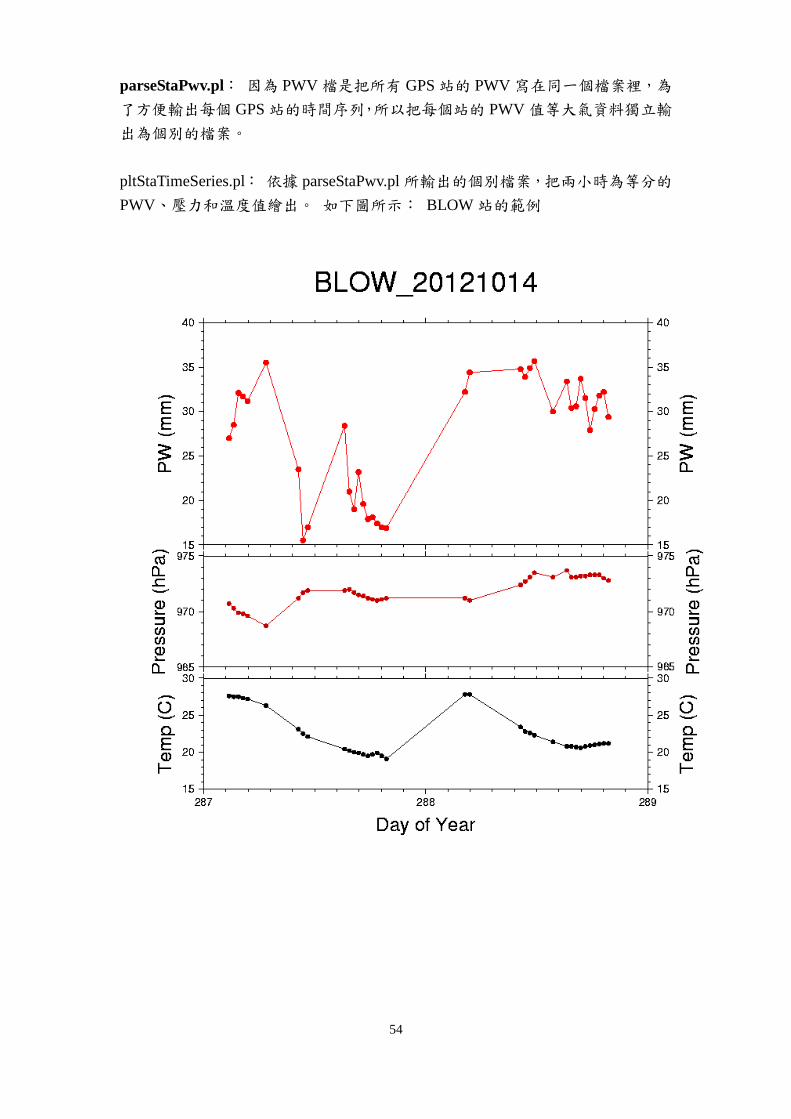
parseStaPwv.pl：因為 PWV檔是把所有 GPS站的 PWV寫在同一個檔案裡，為

了方便輸出每個 GPS站的時間序列，所以把每個站的 PWV值等大氣資料獨立輸

出為個別的檔案。

pltStaTimeSeries.pl：依據 parseStaPwv.pl所輸出的個別檔案，把兩小時為等分的

PWV、壓力和溫度值繪出。如下圖所示： BLOW站的範例

55

附件

出席國際學術會議發表之論文

Applying the water vapor radiometer to verify the

precipitable water vapor measured by GPS

Ta-Kang Yeh1,*

, Jing-Shan Hong2, Chuan-Sheng Wang

1, Tung-Yuan Hsiao

3, Chin-Tzu

Fong2

1 Department of Real Estate and Built Environment, National Taipei University;

[email protected] 2 Meteorological Information Center, Central Weather Bureau

3 Department of Information Technology, Hsing Wu University

Abstract

Taiwan is located at the land-sea interface in a subtropical region. Because the

climate is warm and moist year round, there is a large and highly variable amount of

water vapor in the atmosphere. In addition, because Taiwan is surrounded by ocean

and lacks nearby ground meteorological data, it is difficult to forecast the weather. In

this study, we calculated the Zenith Wet Delay (ZWD) of the troposphere using

ground-based Global Positioning System (GPS). The ZWD measured by a Water

Vapor Radiometer (WVR) was then used to verify the ZWD that had been calculated

using GPS. We also analyzed the correlation between the ZWD and the precipitation

data. We used the observational data from 14 GPS and precipitation stations to

evaluate three cases: one during the plum rain season, a second during binary

typhoons, and a third long duration case. The offset between the GPS-ZWD and the

WVR-ZWD ranged from 1.31 cm to 2.57 cm. The correlation coefficient ranged from

0.89 to 0.93. The results calculated from GPS and those measured using the WVR

were very similar. Moreover, when there was no rain, light rain, moderate rain, or

heavy rain, the flatland station ZWD was 0.31 m, 0.36 m, 0.38 m, or 0.40 m,

respectively. The mountain station ZWD exhibited the same trend. Therefore, these

results have demonstrated that the potential and strength of precipitation in a region

can be estimated according to its ZWD values. If this method can eventually be

expanded to the more than 400 GPS stations in Taiwan and its surrounding islands,

observational data with improved spatial and temporal resolution can be provided to

the city and countryside weather forecasting system that is currently under

development. Such an exchange would fundamentally improve the resources used to

generate weather forecasts.

Keywords: global positioning system, zenith wet delay, water vapor radiometer,

rainfall

56

1. Introduction

Since its development, Global Positioning System (GPS) technology has been

widely used in many fields. The application of GPS technology to the field of

meteorology is called GPS Meteorology (GPS/Met). The primary purpose of this

work was to utilize the delay effect of the GPS satellite signal, which is caused by

Earth’s atmosphere, to derive useful atmospheric information and ultimately

contribute to the development of atmospheric science, meteorology, and other related

fields. Many examples from European and American countries have suggested that

performing near real-time atmosphere monitoring using the GPS tracking network can

positively contribute to long-term climate monitoring and short-term weather

forecasting. Currently, there is an increasing demand for weather forecasting,

especially emergent weather forecasting. By utilizing continuous observation from a

GPS signal, the dynamic variations of precipitation in the troposphere can be

observed. The near real-time continuous nationwide precipitation data, which feature

high precision, as well as high spatial and temporal resolution, can be used in

meteorology research to improve the ability to forecast emergent weather. GPS offers

some advantages when compared with meteorological radar and radiosonde, which

are traditionally used in weather forecasting. Meteorological radar can only measure

the spatial distribution of raindrops, but it cannot measure water vapor distribution.

This drawback greatly weakens its usage for weather forecast warnings. The

radiosonde is a single-use piece of equipment that has low spatial and temporal

resolution; its typical sampling rate is twice daily. Conversely, because ground-based

GPS is inexpensive, it can be densely distributed. GPS technology can provide nearly

real-time, highly precise, and continuously varying Precipitable Water Vapor (PWV)

data across a wide coverage area. This ability is very important for improving the

short-term weather forecast capability, especially in terms of thunderstorm forecasting

and numerical weather forecast models. Currently, the ground-based GPS network of

the National Oceanic and Atmospheric Administration (NOAA) of the United States

can automatically estimate the variation of PWV above the network surface every 30

min. The Japanese GPS network, consisting of more than 1000 stations, has also been

used in functional ground-based GPS meteorological applications (Shoji et al., 2003).

Although GPS can facilitate the ability to make highly precise measurements of

the phases of carrier waves for navigation, the error caused by the atmosphere has

drawn increasing attention. These errors arise due to ionospheric and tropospheric

delays. For the ionosphere delay, the error can be reduced using dual-frequency

observation or simultaneous observation of the differential method. The troposphere

delay consists of two components: the dry component (caused by the temperature and

pressure variations of the dry air, which change the refraction index of the air) and the

57

wet component (caused by the uneven distribution of water vapor, which causes the

signals to refract). The former component can be precisely calculated using ground

pressure detection. However, the latter component cannot be easily corrected because

of the uneven distribution and instability of the atmospheric water vapor. Although the

wet delay of the troposphere is much smaller than the dry delay, the uncertainty of the

troposphere wet delay introduces a lack of predictability into high-precision GPS

applications. Finding an effective solution for the troposphere delay would increase

the precision of GPS positioning and could also be used to derive the PWV of the

atmosphere to provide a near real-time ability to forecast weather.

The atmospheric delay along the path of electromagnetic waves is largely

unknown. Therefore, many models estimate delay values for electromagnetic waves

in the atmosphere using ground meteorological data, the elevation angle, and the

azimuth angle. These delay values differ based on the empirical model from which

they are derived, and the ground meteorology empirical models are primarily used to

estimate the Zenith Wet Delay (ZWD). However, due to the uneven distribution of

water vapor at high altitudes, many questions remain regarding the estimation of

ZWD using ground empirical models (Mendes and Langley, 1999). In this study, we

used a ground-based GPS station to derive ZWD information. We then compared the

ZWD data with observational data from a Water Vapor Radiometer (WVR) to verify

the accuracy of the GPS-ZWD data. The results of this comparison can be used in

industrial fields and to calculate atmospheric PWV. In the future, these results can

provide supporting information that can be used in weather forecasting and in

environmental monitoring.

2. Theory of the Troposphere Delay

The troposphere primarily influences the GPS signal in two ways. The

propagation speed of the signal is slowed down relative to that of a vacuum, and the

signal path is bent rather than straight; both of these effects are caused by refraction

along the path. For the former effect, the refraction index of the troposphere is larger

than that of a vacuum, thereby causing the speed delay. For the latter effect, because

the refraction index varies with altitude, the propagation path is bent and delayed.

These two types of delays, the speed delay and the path delay, are discussed in the

following section.

(1) Speed Delay

Because the refraction index of the troposphere is larger than the refraction index

in a vacuum, electromagnetic waves travel more slowly through the atmosphere than

through a vacuum; this phenomenon is called the propagation time delay. The effect

of this propagation time delay can be estimated as the propagation path is elongated.

The relationship between the speed in a vacuum and that in a medium can be

58

expressed as follows:

n

VV v

M (1)

in which vV is the signal speed in vacuum, n is the refraction index of the medium,

and MV is the signal speed in the medium. The refraction index of the medium

changes along the propagation path because of temperature and pressure variations.

Therefore, the index is a function of the path, and the speed delay Trop

vD due to the

different speeds is expressed as follows:

dssnDTrop

v ]1)([

(2)

(2) Path Delay

Because the refraction index of the atmosphere changes according to the

atmospheric height, an electromagnetic wave that travels through the atmosphere will

have a bent path instead of a straight path. Because a bent path is longer than a

straight line, the path is elongated between the satellite and the receiver. The path

delay Trop

pD is expressed as follows:

GSDTrop

p

(3)

in which S and G represent the straight and bent paths, respectively. In summary, the

troposphere delay TropD can be expressed as follows:

)(]1)([ GSdssnDDD Trop

p

Trop

v

Trop

(4)

In Eq. (4), dssn 1 is the effect of the speed delay, and (S-G) is the effect

of the bent path. In general, the (S-G) delay is less than 1 cm when the elevation angle

is greater than 15°, and it only represents 0.1% of the total delay (Bock and

Doerflinger, 2001). Therefore, this delay can be neglected. The primary factors that

cause the longer path are the different refraction indexes at the different atmospheric

heights. According to Eq. (4), the zenith troposphere delay Z

tropL is as follows:

HH

Z

trop NdzdzznL 6101 (5)

in which the refraction index N can be expressed as follows:

1

232

1

1

wd

d ZT

ek

T

ekZ

T

PkN

(6)

in which N is a function of the temperature, pressure, and water vapor pressure; P d is

the dry air pressure; e is the water vapor pressure; T is the absolute temperature;

59

and are constants; dZ is a dry air compression factor; and wZ is a water

vapor compression factor. Finally, from Eq. (6), we derive the following:

Hd

ws

dm

Z

wtrop

Z

htrop

Z

trop dzT

ek

T

e

M

MkkP

Mg

RkDDL

231216

,, 10 (7)

in which Z

htropD , is the dry delay, Z

wtropD ,is the wet delay, R is a molar gas constant,

mg is the mass center of the vertical air column, dM is the molar weight of the dry air,

wM is the molar weight of the water vapor, and sP is the surface atmosphere pressure.

In Eq. (7), s

dm

PMg

Rk1 (expressed as Z

hL ) is the zenith hydrostatic delay, or the dry

delay, which can be calculated by measuring the total surface atmospheric pressure;

the term Z

Hd

w dT

ek

T

e

M

Mkk

2312(expressed as Z

wL ) is the wet delay, which can

be calculated when the atmospheric temperature and water vapor pressure are known.

Typically, the zenith signal delay caused by neutral atmosphere is approximately 2.3

m. When the signal elevation angle is 5°, the delay caused by the neutral atmosphere

can reach approximately 25 m (Chen and Herring, 1997).

Because the GPS signals pass through media with unknown refraction indexes,

surface meteorological parameters (temperature, humidity, and pressure) are used to

model the troposphere. To date, researchers have developed several troposphere delay

correction models. Among these models, the three most well-known are the

Saastamoinen model, the modified Hopfield model, and the Niell model.

(1) Saastamoinen Model (Saastamoinen, 1973)

Among the many troposphere models that have been developed to eliminate the

troposphere error, the Saastamoinen model is the most widely used to calculate this

delay. It was derived from the ideal gas law and is expressed as follows:

s

z

h PL 002277.0

(8)

Be

TLz

w 05.01255

002277.0

(9)

in which Ps is the surface atmospheric pressure (mb), T is the surface temperature (K),

e is the surface water vapor pressure (mb), and B is the correction factor. By

substituting the temperature, pressure, and humidity into this empirical equation, a

correction for the troposphere delay can be obtained. The dry delay can easily be

calculated by substituting the precise atmospheric pressure into the Saastamoinen

model. The accuracy of this method can be on the order of millimeters (Janes et al.,

60

1991; Chen et al., 2011).

(2) Modified Hopfield Model (Goad and Goodman, 1974)

The modified Hopfield model uses the length of the position vector instead of the

height to calculate the troposphere delay. Assuming that the radius of the Earth is RE,

h is the height between the surface and the wet component of the atmosphere, and hd

is the height between the surface and the dry component of the atmosphere. Therefore,

the corresponding lengths become rd=RE+hd and rw=RE+h. Figure 1 shows the

relative relationship of the geometric path delay. The troposphere delay can be

expressed as follows (Hofmann-Wellenhof et al., 2001):

dsRr

rrNds

Rr

rrND

Path Path Ew

wwv

Ed

dd

trop

4

6

4

6 1010

(10)

in which dN and wvN represent the refraction indexes of the dry and wet components

above the surface, respectively.

(3) Niell Model (Niell, 1996)

For the Niell model, no meteorological parameter is required. The dry

component is calculated from the latitude, the station elevation, and the day of the

year. The wet component can be obtained by entering the latitude of the station. These

terms can be expressed as follows:

100

sinsin

1

sin

1

1

1

1

sin

1

sin

sin

sin

1

1

1

1

)(H

x

c

b

a

c

b

a

c

b

a

c

b

a

D

ht

ht

ht

ht

ht

ht

dry

dry

dry

dry

dry

dry

trop

dry

(11)

wet

wet

wet

wet

wet

wet

trop

wet

c

b

a

c

b

a

D

sin

sin

sin

1

1

1

1 (12)

in which is the elevation angle of the satellite, H is the elevation, km, km, and km.

Only a minor difference exists between the zenith hydrostatic delays that are

calculated from the Hopfield and Saastamoinen models (Bock and Doerflinger, 2001).

The hydrostatic delay calculated from the Saastamoinen model has been verified

many times, and it is known to be accurate to 1 mm or less (Mendes and Langley,

1999; Yeh et al., 2012). Using the standard atmosphere status and the empirical

meteorological model to replace the observation data from the ground station

produces favorable results (Niell, 1996). However, this analysis is only applicable to

61

long-term data analyses in which the impact of emergent weather events has been

reduced. When data are analyzed over many years, climatic variations can be

observed and detected. However, when data are analyzed over the course of a few

hours or a few days, the particular daily atmospheric conditions will lead to variations

in the daily coordinate calculation results.

To convert the ZWD to PWV according to the definition of precipitable water

vapor, the relationship between the ZWD (△SW) and PWV (PW) is as follows:

ww sP (13)

in which is the scale factor and can be calculated as follows:

23

61 10 kTkR mw (14)

in which k2 and k3 are the experimental constants of the atmospheric refraction, such

that hPaKk 79.642 , hPaKk 25

3 10766.3 , and

hPaKMMkkk dw 52.16122 . The molar mass of the water vapor (Mw) is

18.015 g/mol, such that KkgJMRR ww 524.461 . The scale factor is

related to the temperature; it changes with the latitude, the height of the station, the

season, and the weather. Therefore, the method used to determine the temperature is

very important. In 1984, Davis et al. posted a solution and defined the weighted

average temperature as follows:

dhT

edh

T

eT

ss hhm

2

(15)

in which e is the water vapor pressure and T is the atmospheric temperature (K).

Using radiosonde data that have been collected for many years, Bevis (1994) revealed

a linear relationship between the weighted average temperature Tm and the surface

temperature Ts, as follows: Tm=70.2+0.72Ts. The ZWD can then be converted to

PWV.

3. Data Collection and Processing

In this study, we choose the plum rain, the typhoon, and the long-duration

(three-month) seasons for the case studies. Three datasets were used, including GPS

data, precipitation data, and WVR data. The processing steps and the methods that

were used for these three datasets are explained below.

(1) GPS Data

The GPS data in this study were obtained from the following 14 GPS stations:

YMSM, GS10, SHJU, CAOT, TACH, PKGM, SINY, KDNM, YILN, SOFN, TMAM,

LANB, MZUM, and KMNM. The distribution of the stations is shown in Figure 2.

The Bernese 5.0 software program, developed by the University of Bern in

Switzerland, was used to analyze the GPS data. The ZWD was calculated based on

the assumption that the coordinates of the ground points are fixed. During the process

62

of differential calculation, the orbit error and the clock error of the satellite were

corrected using the IGS precise ephemeris. The ionosphere delay error was eliminated

using the L3 linear combination (Yeh et al., 2009). To avoid eliminating the desired

ZWD during the elimination of the common error while performing the differential

calculation, we used the method of long baseline (approximately 2000 km) static

relative positioning to ensure that the obtained ZWD was the absolute value (Liou et

al., 2000). Moreover, to increase the accuracy of the ZWD calculation, the ocean tide

loading correction was applied and the NAO.99b model was used to achieve the

optimal correction effect (Yeh et al., 2011).

Another important issue was the selection of the main station. We tested various

combinations of main stations and distances; these stations were TSKB of Japan,

GUAM of Guam, BJFS of Beijing, DAEJ of Korea, and YUSN of Taiwan. TSKB of

Japan was chosen as the main station because it produced the best result. At distances

longer than 2000 km, the atmospheric status can be treated as uncorrelated between

the two locations. By increasing the baseline distance between the main station and

the calculation station, atmospheric information can be preserved during the

differential calculation, thereby achieving a more accurate ZWD. Furthermore, due to

the adequacy of the data and the comprehensive error correction, the output frequency

of the ZWD was once per hour and 24 times per day per station. In other words, the

temporal resolution of the GPS-deduced ZWD was 1 hr.

(2) Precipitation Data

To match the locations of the GPS stations, the 14 precipitation stations from the

Central Weather Bureau (CWB) rainfall database located nearest to each of the GPS

stations were selected, including Chutzuhu, Taipei, Hsinchu, Taichung, Wuqi, Chiayi,

Alishan, Hengchun, Yilan, Hualien, Taitung, Lanyu, Matzu, and Kinmen. The

precipitation data in this study were provided by the CWB. The time resolution of

these data was also 1 hr; therefore, there were 24 datasets per day. Due to the 8-hr

time difference between the GPS time and the precipitation time (Taiwan local time),

the precipitation time was converted to GPS time prior to analysis.

(3) WVR Data

This study utilized the WVP-1500, which was developed by the Radiometrics

Company in the US; this is a passive WVR that has five observation wavebands

between 22 and 30 GHz. Its observation range can reach up to a 10-km water vapor

cross section, and the single observation time is less than 10 sec. This instrument can

also be used to measure surface temperature, pressure, and relative humidity. Figure 3

shows an architectural diagram of the Radiometrics WVP-1500, which was equipped

with an Azimuth Drive component. The Radiometrics WVP-1500 can provide

measurements at various azimuth angles by tracking GPS satellites through the GPS

satellite ephemeris to scan every observable satellite. Therefore, the PWV liquid

63

water content can be measured to calculate the wet delay caused by the atmosphere.

Moreover, this instrument includes a Rain Effect Mitigation component, which

includes Super Dewblower and Hydrophobic Radome modules; these modules

prevent measurement error due to the adhesion of water drops to the WVR. On a

technical level, the PWV measured by the WVR should be more accurate than

GPS-measured PWV. However, the WVR is very expensive (the Ministry of the

Interior only owns two instruments nationwide). Therefore, we used the

WVR-measured PWV as a standard in this study to verify the accuracy of the

GPS-calculated ZWD. Due to the cost constraints of WVR, however, GPS is an

economical, real-time, wide-coverage observation method.

The WVR data used in this study were provided by the Ministry of the Interior.

The two instruments were installed at the satellite tracking stations of Yangmungshan

(YMSM) and Beigang (PKGM). The original data from the WVR included the date,

time, surface temperature, pressure, and relative humidity. The resolution between

observations was less than 10 sec. Therefore, the volume of WVR data was very large.

To compare the WVR data with the GPS and precipitation data, the WVR data were

averaged hourly and transferred to GPS time automatically using a program. The

correlation analysis was then performed with the GPS-ZWD and the precipitation

data.

4. Case Study and Result Analysis

4.1 Case 1: Plum Rain Season

The plum rain season occurs each May and June in Taiwan. The precipitation of

the plum rain season accounts for ¼ of the total annual precipitation, and it is a major

water resource in Taiwan. However, excessive precipitation can also cause disasters.

The features of the plum rain season can vary between years. Even meteorologists

admit that the predictability accuracy of rainfall during the plum rain season is low

and that the weather is highly variable (Kueh et al., 2009). Therefore, we chose to

study the plum rain season and analyzed the relationship between the precipitation

observed during the season and the GPS-ZWD. A time period that included Modified

Julian Day (MJD) 53887-53901 (June 1–14) was chosen for this case study. Based on

the information provided on the CWB website, most of the areas in Taiwan

experienced continuous rainfall during MJD 53887–53899. The central and southern

areas experienced torrential and extremely torrential rain, respectively. Some disasters

occurred as a result of the continuous heavy or torrential rainfalls. During this period,

the most notable rainfalls occurred between MJD 53896 and 53897. Starting at MJD

53900, the weather front began to move north. The weather in Taiwan shifted to the

summer type, which is controlled by the Pacific High and involves higher daily

temperatures. The rain system changed primarily to thermal convection, which

64

developed after noon (CWB, 2011).

This case included 14 stations. We first chose the Yangmungshan station and

Beigang station as examples because GPS and WVR data are available for both

stations. In Figure 4, the red line represents the wet delay as measured by the WVR,

the green line represents the wet delay as calculated from the GPS data, the blue line

represents the surface precipitation, and the gray line represents the surface humidity.

From Figure 4, we determined that the ZWD measured by the WVR (referred to as

WVR-ZWD) and the ZWD calculated from GPS data (referred to as GPS-ZWD)

displayed the same trend. The correlation coefficient between the GPS-ZWD and the

WVR-ZWD was 0.96, which suggests that these two sources are highly correlated.

Furthermore, by calculating the difference between the GPS-ZWD and WVR-ZWD

and then averaging the absolute values of these differences, the average discrepancy

between the two ZWDs was found to be 1.19 cm. This result preliminarily verified the

reliability of the ZWD as calculated from the GPS data. The trends of the GPS result

and the WVR result were found to be consistent. Minor system error exists between

the two results.

The result of the PKGM station is shown in Figure 5. The difference between the

WVR-ZWD and GPS-ZWD was relatively larger than that at the YMSM station. The

correlation coefficient was only 0.77, which is a much poorer correlation than that

observed at the YMSM station. Upon further analysis, we found that the results of the

red line (WVR-ZWD) and the green line (GPS-ZWD) are broadly similar. However,

they do not coincide with each other from MJD 53895–53896, which were the two

days with heavy rainfall. During these two days, the average precipitation was more

than 20 mm/hr, which is considered to be torrential rain. Therefore, the observed

ZWD should have synchronously increased. However, the red line (measured by

WVR) decreased while the green line (calculated from the GPS data) increased. This

result suggests that the GPS is more reliable than the WVR during heavy rainfall. This

strong rainfall period was the primary reason for the low correlation coefficient. If we

excluded this period, the correlation coefficient between the GPS-ZWD and the

WVR-ZWD was 0.9, which is highly correlated. Moreover, by using the method used

for YMSM station to calculate the absolute values of the differences, the average

discrepancy between the GPS-ZWD and WVR-ZWD was 1.42 cm. This result

suggests that a relatively larger system error exists between the GPS-ZWD and

WVR-ZWD data when the rainfall intensity is large.

4.2 Case 2: Two Typhoons

This case encompassed MJD 53950–53961 (August 3–13). Seven typhoons

occurred in August of that year. We choose the Bopha and Saomai typhoons as

examples. Typhoon Bopha formed in the eastern sea of Taiwan. The maximum wind

65

speed near the typhoon center was 23.0 m/s. The landing point was in eastern Taiwan.

The CWB activated the typhoon landing alarm on MJD 53955. The intermittent, large

rainfall brought by Bopha (the total precipitation was approximately 250 mm in the

mountain area) caused crop damage. Typhoon Saomai formed in the southwest sea of

Guam. The maximum wind speed near the typhoon center was 48.0 m/s. The CWB

activated the typhoon landing alarm on MJD 53956. Due to the rapid speed of Saomai,

the warning time was short. Moreover, the cloud cluster was dense and concentrated

within the storm circle. Only northern Taiwan, which was passed by the storm circle,

experienced relatively strong wind and intermittent rainfalls during the morning of

MJD 53957. The CWB cancelled the alarm in the afternoon on MJD 53957.

The data used in this case study were also derived from the GPS and

precipitation stations. The YMSM and PKGM stations also produced the WVR data.

Figure 6 shows similar trends to those observed in Case 1. At the YMSM station, the

ZWD calculated from the GPS data and the ZWD measured by the WVR showed the

same trend. The correlation coefficient was 0.93. The average discrepancy was 2.47

cm. Both the correlation coefficient and the discrepancy were worse than the values

calculated for the plum rain season case. This result may have been caused by the

severe weather changes that occurred during the typhoon period, which decreased the

accuracy of the ZWD calculation. Figure 6 clearly shows that the ZWD increased

rapidly when the typhoon was approaching and decreased rapidly as the typhoon left.

The hourly precipitation reached its maximum on MJD 53957. The GPS-ZWD and

WVR-ZWD reached peak levels simultaneously. Two days after the typhoon (MJD

53959), the ZWD rapidly decreased to its minimum during the period.

We next analyzed the data from the PKGM station. Figure 7 shows that after the

first typhoon began to affect Taiwan (MJD 53955), the observation data from the

WVR became erratic. Further investigation revealed that the abnormal data were

caused by a servomotor failure. The WVR uses the servomotor to rotate the

equipment to track the GPS satellites. However, the servomotor failed because of the

strong wind produced by the typhoon. Therefore, the measured data were incorrect.

Prior to the servomotor failure, the GPS-calculated ZWD and the WVR-measured

ZWD displayed the same trend. When the data after MJD 53955 were excluded, the

correlation coefficient between the GPS-ZWD and the WVR-ZWD was calculated to

be 0.85. The average discrepancy was 2.67 cm. Both of these parameters were worse

than those calculated in the plum rain season case, which was similar to the YMSM

station. This result again suggests that the accuracy of the ZWD is reduced during the

typhoon period. Figure 7 also shows that the GPS-ZWD increased rapidly when the

two typhoons were closest to Taiwan (MJD 53957 and 53957). After the typhoons,

the GPS-ZWD decreased rapidly. One day after the typhoons (MJD 53958), the

GPS-ZWD decreased rapidly to its minimum value of the period.

66

4.3 Case 3: Long Duration

The long-duration case used three months of data, from MJD 53826 to 53917

(April-June). We used the same stations as in the previous two cases. Figure 8 shows

the result of the YMSM station. We can see that the long-duration and short-duration

cases (Case 3 and Case 1) are similar. The ZWD measured by the WVR and the ZWD

calculated from GPS displayed the same trend. The correlation coefficient was 0.94,

and the average difference was 1.26 cm. Both of these parameters were better than

those of the typhoon case but slightly worse than those of the plum rain season case.

By comparing the precipitation and the ZWD, we found that the delay increases

dramatically when a rainfall occurs, whereas the wet delay decreases rapidly

following a rainfall.

Figure 9 shows the result of the PKGM station. During the period from April to

June, the majority of the precipitation clearly occurred in June in southern Taiwan.

The correlation coefficient between the WVR-ZWD and GPS-ZWD was 0.91, and the

average difference was 1.89 cm. This result is better than those of the two

short-duration cases. Compared with the typhoon case, the improved results in the

long-duration case may be caused by the low GPS accuracy, which resulted from the

severe change that occurred in the atmosphere during the typhoon period. In the plum

rain case, the PKGM station was located in an area that experienced extremely

torrential rainfall (the hourly precipitation was 20–60 mm). Therefore, the

inaccuracies could be attributed to the larger observational error of the WVR.

After verifying the precipitable water vapor that was calculated from the GPS

data using the WVR data, we further analyzed the relationship between the ZWD and

precipitation by dividing the long-duration data into two types, those with

precipitation and those without precipitation (see Table 1). We also separated the

stations into flatland and mountain stations. The stations were then ranked according

to their latitudes. Table 1 shows that the ZWD threshold of precipitation for the

flatland stations was 0.36 m, whereas it was only 0.31 m for the mountain stations.

This is a difference of 0.05 m, which represents 14% of the total. The same

phenomenon was observed in the data without precipitation. The average ZWDs of

the flatland stations and mountain stations were 0.31 m and 0.27 m, respectively. The

difference was 0.04 m, which represents 13% of the total. Therefore, the height of the

station must be considered when using the ZWD to predict whether rainfall will occur.

The reasoning is as follows: because the mountain station is located at a higher

altitude, the layer of troposphere through which the GPS signal passes to reach the

GPS receivers is thinner for the mountain station than for the flatland station.

Therefore, the error of the signal due to the water vapor delay is smaller. Conversely,

the GPS signals must pass through a thicker layer of troposphere before reaching the

67

flatland stations. Therefore, the signal delay effect at the flatland stations is larger

than that at the mountain stations.

Next, according to the amount of rainfall, we divided the data into heavy rain,

moderate rain, and light rain categories to investigate the correlation between the

ZWD and the rainfall strength. Table 2 shows the three categories. The definitions of

the three categories are as follows: heavy rain refers to rainfall with an hourly

precipitation rate above 20 mm, moderate rain refers to rainfall with an hourly

precipitation rate between 10 mm and 20 mm, and light rain refers to rainfall with an

hourly precipitation rate of less than 10 mm. Table 2 shows that when light rain

occurred at the flatland stations, the average ZWD was 0.36 m; when moderate rain

occurred, the average ZWD increased to 0.38 m. The difference was 0.02 m, which

represents 5% of the total. When heavy rain occurred, the average ZWD reached 0.40

m. The difference between the heavy rain and moderate rain was 0.02 m, which

represents 5% of the total. When light rain, moderate rain, and heavy rain occurred at

the mountain stations, the corresponding ZWD values were 0.30 m, 0.33 m, and 0.34

m, respectively. The increase was only slightly different than that at the flatland

stations. Based on the aforementioned results, we concluded that at regions with

different elevations, the GPS-ZWD cannot be used alone to decide whether a potential

for precipitation exists; the value of the GPS-ZWD should also be used to decide the

strength of the precipitation. Recently, the CWB has applied ground-based GPS to

calculate near real-time ZWD data. By importing these data into the numerical

meteorological model, encouraging preliminary results have been obtained (Kuo et al.,

2000; Chen et al., 2009). If this method can be applied to all 400+ GPS stations in

Taiwan and its surrounding islands, higher spatial- and temporal-resolution data can

be provided to the city and countryside weather forecast system currently under

development. Consequently, the quality of the fundamental resources that are used in

weather forecasting can be improved.

5. Conclusions and Recommendations

In this study, we utilized ground-based GPS signals to calculate the ZWD. The

accuracy of the GPS-ZWD was verified using the ZWD that was measured by the

WVR. Based on the averaged data from the YMSM and PKGM stations, the

difference between the GPS-ZWD and WVR-ZWD was 1.31 cm in the plum rain

season case. The correlation coefficient was 0.93. In the typhoon case, the difference

between the GPS-ZWD and WVR-ZWD was 2.57 cm, and the correlation coefficient

was 0.89. In the long-duration case, the difference between the GPS-ZWD and

WVR-ZWD was 1.58 cm, and the correlation coefficient was 0.93. Assuming that the

WVR-ZWD is true to evaluate the accuracy of the GPS-ZWD, we observed only

minimal differences between the long-duration and plum rain season cases. However,

68

the accuracy obtained during the typhoon case was notably reduced. This reduction

could be related to the 1-hr resolution of the ZWD. In other words, we assumed that

the ZWD does not change significantly over the course of an hour. Therefore, a

constant unknown was given and solved. However, because atmospheric parameters

can change rapidly during a typhoon period, the ZWD cannot be a fixed value.

Therefore, the accuracy of the GPS-ZWD was lower in the typhoon case. In the future,

30- or even 15-min time resolutions may be used to calculate the ZWD. However, a

higher time resolution may also induce too many unknowns, which may lead to an

unsolvable problem or to decreased accuracy. Moreover, although the WVR is

equipped with the Rain Effect Mitigation component, the observational data derived

from the WVR were notably abnormal when the rate of rainfall was greater than 20

mm/hr. This phenomenon could be related to the measurement error caused by the

water drops adhering to the surface of WVR during periods of heavy rainfall.

Therefore, during heavy rainfall, GPS data are more reliable than WVR data.

In this study, we also observed that rainfall can occur at flatland stations when

the average ZWD value reaches 0.36 m; at the mountain stations, this value is 0.31 m.

The difference between the values is 0.05 m, which represents 14% of the total.

Therefore, the height of the station must be considered when the ZWD is used to

decide whether a certain area will experience rainfall. Furthermore, when the flatland

stations experienced light rain, moderate rain, and heavy rain, the ZWDs were 0.36 m,

0.38 m, and 0.40 m, respectively. For the mountain stations, the ZWDs were 0.30 m,

0.33 m, and 0.45 m, respectively. This result suggests that at different elevations, the

ZWD value can be used to forecast the potential for and strength of precipitation. The

GPS calculation method that was used in this study, long baseline static relative

positioning, was used to eliminate many common system errors. Although this

method can generate a higher accuracy for the ZWD calculation, the accuracy greatly

depends on the main station. In the future, if the Precise Point Positioning (PPP)

method can be revised to improve the accuracy of the error correction, the absolute

and independent ZWD value can be obtained; this goal will be the focus of our future

studies.

References

Bevis, M., 1994. GPS meteorology: mapping zenith wet delays onto precipitable

water, Journal of Application Meteorology, 33, 379-386.

Bock, O. and Doerflinger, E., 2001. Atmospheric modeling in GPS data analysis for

high accuracy positioning, Phys. Chem. Earth (A), 26(6-8), 373-383.

Chen, C. H., Yeh, T. K., Liu, J. Y., Wang, C. H., Wen, S., Yen, H. Y., and Chang, S. H.,

2011. Surface deformation and seismic rebound: implications and applications,

Surveys in Geophysics, 32(3), 291-313, doi: 10.1007/s10712-011-9117-3.

Chen, G. and Herring, T. A., 1997. Effects of atmospheric azimuthal asymmetry on the

analysis of space geodetic data, J. Geophys. Res., 102(20), 489-502.

Chen, S. Y., Huang, C. Y., Kuo, Y. H., Guo, Y. R. and Sokolovskiy, S., 2009.

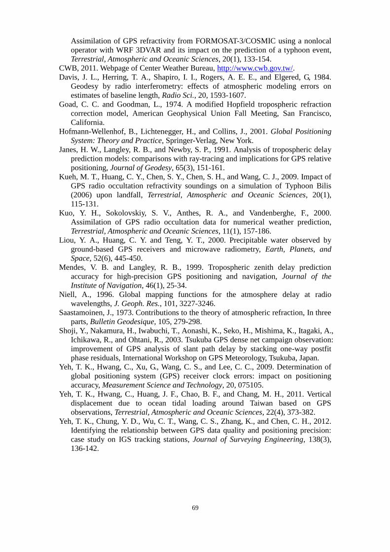
69

Assimilation of GPS refractivity from FORMOSAT-3/COSMIC using a nonlocal

operator with WRF 3DVAR and its impact on the prediction of a typhoon event,

Terrestrial, Atmospheric and Oceanic Sciences, 20(1), 133-154.

CWB, 2011. Webpage of Center Weather Bureau, http://www.cwb.gov.tw/.

Davis, J. L., Herring, T. A., Shapiro, I. I., Rogers, A. E. E., and Elgered, G, 1984.

Geodesy by radio interferometry: effects of atmospheric modeling errors on

estimates of baseline length, Radio Sci., 20, 1593-1607.

Goad, C. C. and Goodman, L., 1974. A modified Hopfield tropospheric refraction

correction model, American Geophysical Union Fall Meeting, San Francisco,

California.

Hofmann-Wellenhof, B., Lichtenegger, H., and Collins, J., 2001. Global Positioning

System: Theory and Practice, Springer-Verlag, New York.

Janes, H. W., Langley, R. B., and Newby, S. P., 1991. Analysis of tropospheric delay

prediction models: comparisons with ray-tracing and implications for GPS relative

positioning, Journal of Geodesy, 65(3), 151-161.

Kueh, M. T., Huang, C. Y., Chen, S. Y., Chen, S. H., and Wang, C. J., 2009. Impact of

GPS radio occultation refractivity soundings on a simulation of Typhoon Bilis

(2006) upon landfall, Terrestrial, Atmospheric and Oceanic Sciences, 20(1),

115-131.

Kuo, Y. H., Sokolovskiy, S. V., Anthes, R. A., and Vandenberghe, F., 2000.

Assimilation of GPS radio occultation data for numerical weather prediction,

Terrestrial, Atmospheric and Oceanic Sciences, 11(1), 157-186.

Liou, Y. A., Huang, C. Y. and Teng, Y. T., 2000. Precipitable water observed by

ground-based GPS receivers and microwave radiometry, Earth, Planets, and

Space, 52(6), 445-450.

Mendes, V. B. and Langley, R. B., 1999. Tropospheric zenith delay prediction

accuracy for high-precision GPS positioning and navigation, Journal of the

Institute of Navigation, 46(1), 25-34.

Niell, A., 1996. Global mapping functions for the atmosphere delay at radio

wavelengths, J. Geoph. Res., 101, 3227-3246.

Saastamoinen, J., 1973. Contributions to the theory of atmospheric refraction, In three

parts, Bulletin Geodesique, 105, 279-298.

Shoji, Y., Nakamura, H., Iwabuchi, T., Aonashi, K., Seko, H., Mishima, K., Itagaki, A.,

Ichikawa, R., and Ohtani, R., 2003. Tsukuba GPS dense net campaign observation:

improvement of GPS analysis of slant path delay by stacking one-way postfit

phase residuals, International Workshop on GPS Meteorology, Tsukuba, Japan.

Yeh, T. K., Hwang, C., Xu, G., Wang, C. S., and Lee, C. C., 2009. Determination of

global positioning system (GPS) receiver clock errors: impact on positioning

accuracy, Measurement Science and Technology, 20, 075105.

Yeh, T. K., Hwang, C., Huang, J. F., Chao, B. F., and Chang, M. H., 2011. Vertical

displacement due to ocean tidal loading around Taiwan based on GPS

observations, Terrestrial, Atmospheric and Oceanic Sciences, 22(4), 373-382.

Yeh, T. K., Chung, Y. D., Wu, C. T., Wang, C. S., Zhang, K., and Chen, C. H., 2012.

Identifying the relationship between GPS data quality and positioning precision:

case study on IGS tracking stations, Journal of Surveying Engineering, 138(3),

136-142.

http://www.cwb.gov.tw/

70

Figure 1: The relative relationship for the geometric path delay of the troposphere.

Figure 2: The distribution of the GPS observation stations.

Atmosphere

Ground

Earth center

71

Figure 3: Architectural diagram of the Radiometrics WVP-1500.

Figure 4: The GPS-ZWD, WVR-ZWD, relative humidity, and precipitation data from

the YMSM station during the plum rain season.

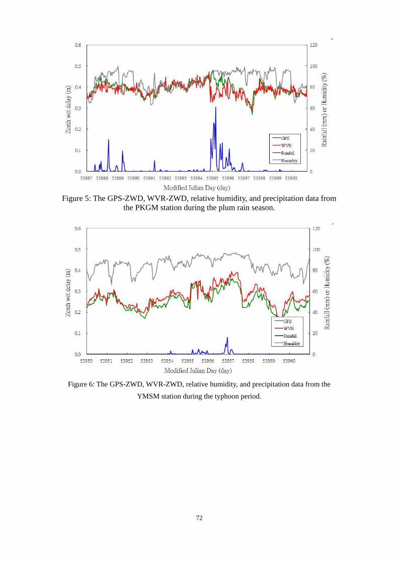
72

Figure 5: The GPS-ZWD, WVR-ZWD, relative humidity, and precipitation data from

the PKGM station during the plum rain season.

Figure 6: The GPS-ZWD, WVR-ZWD, relative humidity, and precipitation data from the

YMSM station during the typhoon period.

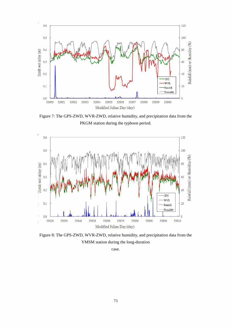
73


PKGM station during the typhoon period.


YMSM station during the long-duration

case.

74


PKGM station during the long-duration case.

Table 1: The average ZWD with and without rainfall from the flatland and mountain

stations

Flatland station Latitude Height

(m)

With rainfall

ZWD (m)

Without rainfall

ZWD (m)

MZUM 26°09’N 60 0.35 0.28

GS10 25°08’N 52 0.35 0.31

SHJU 24°50’N 24 0.36 0.31

YILN 24°44’N 64 0.35 0.32

KMNM 24°24’N 49 0.37 0.31

TACH 24°17’N 34 0.37 0.32

CAOT 23°58’N 142 0.37 0.31

SOFN 23°52’N 59 0.37 0.32

PKGM 23°34’N 43 0.38 0.32

TMAM 22°37’N 59 0.37 0.31

KDMN 21°57’N 58 0.37 0.32

Average 59 0.36 0.31

Mountain station Latitude Height

(m)

With rainfall

ZWD (m)

Without rainfall

ZWD (m)

YMSM 25°10’N 784 0.29 0.25

SINY 23°41’N 536 0.33 0.28

LANB 22°02’N 351 0.32 0.28

Average 557 0.31 0.27

75

Table 2: The average ZWD during different rainfall strengths from the flatland and

mountain stations

Flatland station Latitude Height

(m)

Light rain

ZWD (m)

Moderate rain

ZWD (m)

Heavy rain

ZWD (m)

MZUM 26°09’N 60 0.36 0.37 0.38

GS10 25°08’N 52 0.35 0.38 0.40

SHJU 24°50’N 24 0.36 0.37 0.40

YILN 24°44’N 64 0.35 0.39 0.40

KMNM 24°24’N 49 0.37 0.38 0.38

TACH 24°17’N 34 0.37 0.39 0.40

CAOT 23°58’N 142 0.36 0.39 0.39

SOFN 23°52’N 59 0.36 0.42 0.40

PKGM 23°34’N 43 0.38 0.39 0.42

TMAM 22°37’N 59 0.37 0.39 0.42

KDMN 21°57’N 58 0.36 0.36 0.41

Average 59 0.36 0.38 0.40

Mountain Station Latitude Height

(m)

Light rain

ZWD (m)

Moderate rain

ZWD (m)

Heavy rain

ZWD (m)

YMSM 25°10’N 784 0.28 0.31 0.31

SINY 23°41’N 536 0.32 0.34 0.36

LANB 22°02’N 351 0.31 0.33 0.36

Average 557 0.30 0.33 0.34

Documents

交通部中央氣象局 委託研究計畫期末成果報告 地基 GPS衛星資料 …photino.cwb.gov.tw/rdcweb/lib/cd/cd03cons/Y101_report/101m10.pdf · 委託研究計畫期末成果報告

交通部中央氣象局委託研究計畫期末成果報告地基 GPS衛星資料 …photino.cwb.gov.tw/rdcweb/lib/cd/cd03cons/Y101_report/101m10.pdf · 委託研究計畫期末成果報告