Embed Size (px)
Citation preview
EECS 247 Lecture 2: Filters © 2010 Page 1
EE247 - Lecture 2Filters
• Filters: – Nomenclature
– Specifications• Quality factor
• Magnitude/phase response versus frequency characteristics
• Group delay
– Filter types• Butterworth
• Chebyshev I & II
• Elliptic
• Bessel
– Group delay comparison example
– Biquads
EECS 247 Lecture 2: Filters © 2010 Page 2
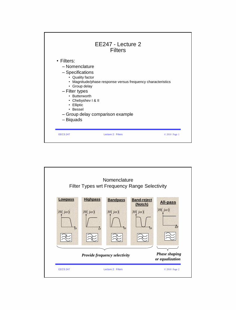
Nomenclature
Filter Types wrt Frequency Range Selectivity
jH jH
Lowpass Highpass Bandpass Band-reject
(Notch)
Provide frequency selectivity
jH jH
All-pass
jH
Phase shaping
or equalization

EECS 247 Lecture 2: Filters © 2010 Page 3
Filter Specifications
• Magnitude response versus frequency characteristics:
– Passband ripple (Rpass)
– Cutoff frequency or -3dB frequency
– Stopband rejection
– Passband gain
• Phase characteristics:
– Group delay
• SNR (Dynamic range)
• SNDR (Signal to Noise+Distortion ratio)
• Linearity measures: IM3 (intermodulation distortion), HD3 (harmonic distortion), IIP3 or OIP3 (Input-referred or output-referred third order intercept point)
• Area/pole & Power/pole
EECS 247 Lecture 2: Filters © 2010 Page 4
0
x 10Frequency (Hz)
Filter Magnitude versus Frequency CharacteristicsExample: Lowpass
jH
jH
0H
Passband Ripple (Rpass)
Transition Band
cf
Passband
Passband
Gain
stopfStopband
Frequency
Stopband Rejection
f
H j [dB]
3dBf
dB3

EECS 247 Lecture 2: Filters © 2010 Page 5
Filters
• Filters:
– Nomenclature
– Specifications• Magnitude/phase response versus frequency characteristics
• Quality factor
• Group delay
– Filter types• Butterworth
• Chebyshev I & II
• Elliptic
• Bessel
– Group delay comparison example
– Biquads
EECS 247 Lecture 2: Filters © 2010 Page 6
Quality Factor (Q)
• The term quality factor (Q) has different
definitions in different contexts:
–Component quality factor (inductor &
capacitor Q)
–Pole quality factor
–Bandpass filter quality factor
• Next 3 slides clarifies each

EECS 247 Lecture 2: Filters © 2010 Page 7
Component Quality Factor (Q)
• For any component with a transfer function:
• Quality factor is defined as:
Energy Storedper uni t t ime
Average Power Dissipat ion
1H jR jX
XQ
R
EECS 247 Lecture 2: Filters © 2010 Page 8
Component Quality Factor (Q)
Inductor & Capacitor Quality Factor
• Inductor Q :
Rs series parasitic resistance
• Capacitor Q :
Rp parallel parasitic resistance
RsL
s sL L
1 LY QR j L R
Rp
C
pC C
p
1Z Q CR1 j
RC

EECS 247 Lecture 2: Filters © 2010 Page 9
Pole Quality Factor
x
x
j
P
pPol e
x
Q 2
s-Plane• Typically filter
singularities include
pairs of complex
conjugate poles.
• Quality factor of
complex conjugate
poles are defined as:
EECS 247 Lecture 2: Filters © 2010 Page 10
Bandpass Filter Quality Factor (Q)
0.1 1 10f1 fcenter f2
0
-3dB
Df = f2 - f1
H jf
Frequency
Magn
itu
de
[dB
]
Q fcenter /Df

EECS 247 Lecture 2: Filters © 2010 Page 11
Filters
• Filters:
– Nomenclature
– Specifications• Magnitude/phase response versus frequency characteristics
• Quality factor
• Group delay
– Filter types• Butterworth
• Chebyshev I & II
• Elliptic
• Bessel
– Group delay comparison example
– Biquads
EECS 247 Lecture 2: Filters © 2010 Page 12
• Consider a continuous-time filter with s-domain transfer function G(s):
• Let us apply a signal to the filter input composed of sum of two sine
waves at slightly different frequencies (D):
• The filter output is:
What is Group Delay?
vIN(t) = A1sin(t) + A2sin[(+D) t]
G(j) G(j)ej()
vOUT(t) = A1 G(j) sin[t+()] +
A2 G[ j(+D)] sin[(+D)t+ (+D)]

EECS 247 Lecture 2: Filters © 2010 Page 13
What is Group Delay?
{ ]}[vOUT(t) = A1 G(j) sin t + ()
+
{ ]}[+ A2 G[ j(+D)] sin (+D) t +(+D)
+D
(+D)
+D ()+
d()
dD[ ][
1
)( ]1 -D
d()
d
()
+()
-( ) D
D
<<1Since then D
0[ ]2
EECS 247 Lecture 2: Filters © 2010 Page 14
What is Group Delay?
Signal Magnitude and Phase Impairment
{ ]}[vOUT(t) = A1 G(j) sin t + ()
+
{ ]}[+ A2 G[ j(+D)]sin (+D) t +d()
d
()
+()
-( )D
• PD -()/ is called the “phase delay” and has units of time
• If the delay term d is zero the filter’s output at frequency +D and the output at frequency are each delayed in time by -()/
• If the term d is non-zerothe filter’s output at frequency +D is time-shifted differently than the filter’s output at frequency
“Phase distortion”
d
EECS 247 Lecture 2: Filters © 2010 Page 15
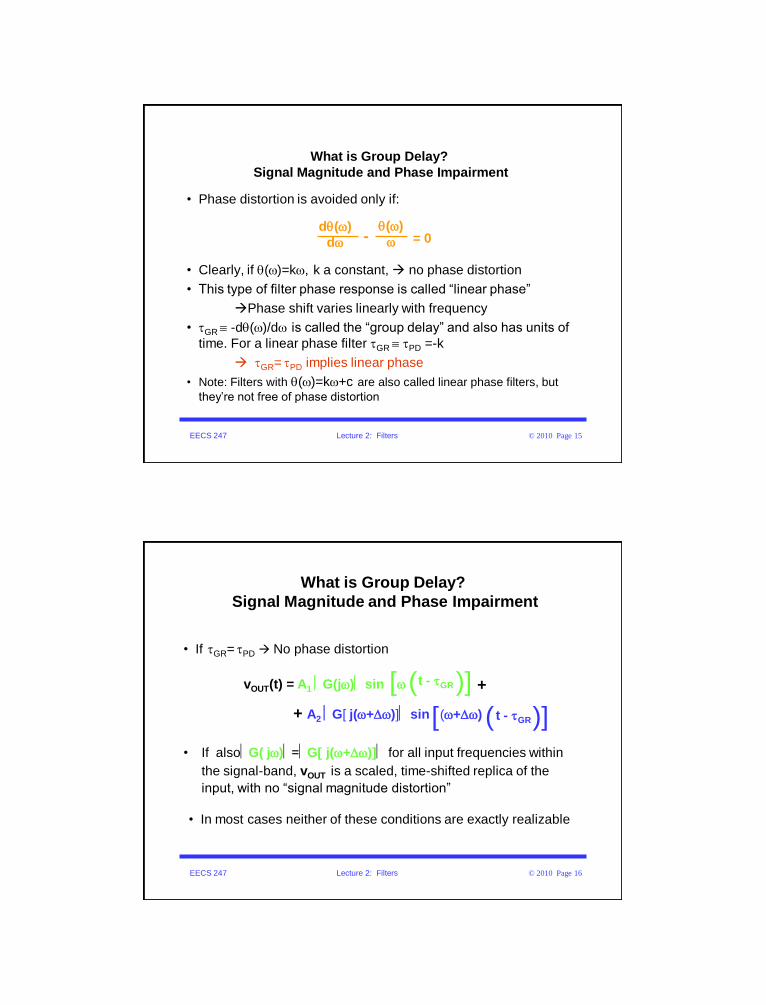
• Phase distortion is avoided only if:
• Clearly, if ()=k, k a constant, no phase distortion
• This type of filter phase response is called “linear phase”
Phase shift varies linearly with frequency
• GR -d()/d is called the “group delay” and also has units of
time. For a linear phase filter GR PD =-k
GR= PD implies linear phase
• Note: Filters with ()=k+c are also called linear phase filters, but
they’re not free of phase distortion
What is Group Delay?
Signal Magnitude and Phase Impairment
d()
d
()
- = 0
EECS 247 Lecture 2: Filters © 2010 Page 16
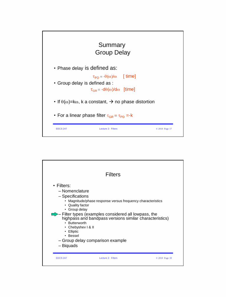
What is Group Delay?
Signal Magnitude and Phase Impairment
• If GR= PD No phase distortion
[ )](vOUT(t) = A1 G(j) sin t - GR +
[+ A2 G[ j(+D)] sin (+D) )]( t - GR
• If alsoG( j)=G[ j(+D)] for all input frequencies within
the signal-band, vOUT is a scaled, time-shifted replica of the
input, with no “signal magnitude distortion”
• In most cases neither of these conditions are exactly realizable
EECS 247 Lecture 2: Filters © 2010 Page 17
• Phase delay is defined as:
PD -()/ [ time]
• Group delay is defined as :
GR -d()/d [time]
• If ()=k, k a constant, no phase distortion
• For a linear phase filter GR PD =-k
Summary
Group Delay
EECS 247 Lecture 2: Filters © 2010 Page 18
Filters
• Filters: – Nomenclature
– Specifications • Magnitude/phase response versus frequency characteristics
• Quality factor
• Group delay
– Filter types (examples considered all lowpass, the highpass and bandpass versions similar characteristics)
• Butterworth
• Chebyshev I & II
• Elliptic
• Bessel
– Group delay comparison example
– Biquads

EECS 247 Lecture 2: Filters © 2010 Page 19
Filter Types wrt Frequency Response
Lowpass Butterworth Filter
• Maximally flat amplitude within
the filter passband
• Moderate phase distortion
-60
-40
-20
0
Ma
gn
itu
de (
dB
)1 2
-400
-200
Normalized Frequency P
ha
se (
deg
rees)
5
3
1
No
rmalized
Gro
up
Dela
y
0
0
Example: 5th Order Butterworth filter
N
0
d H( j )0
d
EECS 247 Lecture 2: Filters © 2010 Page 20
Lowpass Butterworth Filter
• All poles
• Number of poles equal to filter
order
• Poles located on the unit
circle with equal angles
s-plane
j
Example: 5th Order Butterworth Filter
pole

EECS 247 Lecture 2: Filters © 2010 Page 21
Filter Types
Chebyshev I Lowpass Filter
• Chebyshev I filter
– Ripple in the passband
– Sharper transition band
compared to Butterworth (for
the same number of poles)
– Poorer group delay
compared to Butterworth
– More ripple in passband
poorer phase response
1 2
-40
-20
0
Normalized Frequency
Ma
gn
itu
de [
dB
]
-400
-200
0
Ph
as
e [
de
gre
es
]
0
Example: 5th Order Chebyshev filter
35
0 No
rma
lize
d G
rou
p D
ela
y
EECS 247 Lecture 2: Filters © 2010 Page 22
Chebyshev I Lowpass Filter Characteristics
• All poles
• Poles located on an ellipse inside
the unit circle
• Allowing more ripple in the
passband:
_Narrower transition band
_Sharper cut-off
_Higher pole Q
_Poorer phase response
Example: 5th Order Chebyshev I Filter
s-planej
Chebyshev I LPF 3dB passband ripple
Chebyshev I LPF 0.1dB passband ripple
EECS 247 Lecture 2: Filters © 2010 Page 23
Normalized Frequency
Ph
ase (
deg
)M
ag
nit
ud
e (
dB
)
0 0.5 1 1.5 2
-360
-270
-180
-90
0
-60
-40
-20
0
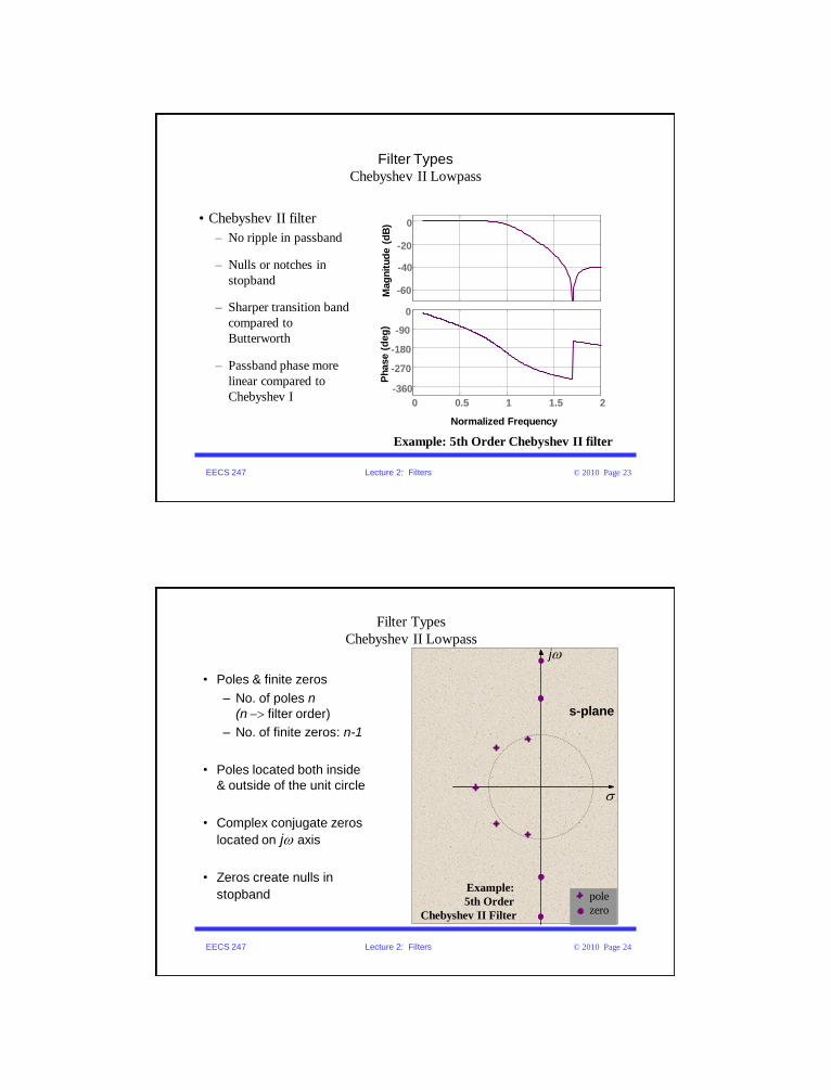
Filter Types
Chebyshev II Lowpass
• Chebyshev II filter
– No ripple in passband
– Nulls or notches in
stopband
– Sharper transition band
compared to
Butterworth
– Passband phase more
linear compared to
Chebyshev I
Example: 5th Order Chebyshev II filter
EECS 247 Lecture 2: Filters © 2010 Page 24
Filter Types
Chebyshev II Lowpass
Example:
5th Order
Chebyshev II Filter
s-plane
j
• Poles & finite zeros
– No. of poles n
(n filter order)
– No. of finite zeros: n-1
• Poles located both inside
& outside of the unit circle
• Complex conjugate zeros
located on j axis
• Zeros create nulls in
stopband pole
zero
EECS 247 Lecture 2: Filters © 2010 Page 25
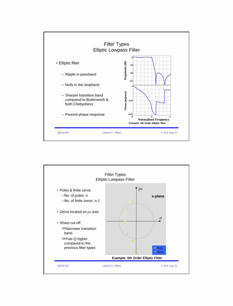
Filter Types
Elliptic Lowpass Filter
• Elliptic filter
– Ripple in passband
– Nulls in the stopband
– Sharper transition band
compared to Butterworth &
both Chebyshevs
– Poorest phase response
Ma
gn
itu
de (
dB
)Example: 5th Order Elliptic filter
-60
1 2
Normalized Frequency0
-400
-200
0
Ph
as
e (
de
gre
es
)
-40
-20
0
EECS 247 Lecture 2: Filters © 2010 Page 26
Filter Types
Elliptic Lowpass Filter
Example: 5th Order Elliptic Filter
s-plane
j
• Poles & finite zeros
– No. of poles: n
– No. of finite zeros: n-1
• Zeros located on j axis
• Sharp cut-off
_Narrower transition
band
_Pole Q higher
compared to the
previous filter types Pole
Zero

EECS 247 Lecture 2: Filters © 2010 Page 27
Filter Types
Bessel Lowpass Filter
s-planej
• Bessel
–All poles
–Poles outside unit circle
–Relatively low Q poles
–Maximally flat group delay
–Poor out-of-band attenuation
Example: 5th Order Bessel filter
Pole
EECS 247 Lecture 2: Filters © 2010 Page 28
Magnitude Response Behavior
as a Function of Filter Order
Example: Bessel Filter
Normalized Frequency
Mag
nit
ud
e [
dB
]
0.1 100-100
-90
-80
-70
-60
-50
-40
-30
-20
-10
0
n=1
2
3
4
5
7
6
1 10
n Filter order

EECS 247 Lecture 2: Filters © 2010 Page 29
Filter Types
Comparison of Various Type LPF Magnitude Response
-60
-40
-20
0
Normalized Frequency
Magn
itu
de (
dB
)
1 20
Bessel
Butterworth
Chebyshev I
Chebyshev II
Elliptic
All 5th order filters with same corner freq.
Ma
gn
itu
de
(d
B)
EECS 247 Lecture 2: Filters © 2010 Page 30
Filter Types
Comparison of Various LPF Singularities
s-plane
j
Poles Bessel
Poles Butterworth
Poles Elliptic
Zeros Elliptic
Poles Chebyshev I 0.1dB

EECS 247 Lecture 2: Filters © 2010 Page 31
Comparison of Various LPF Groupdelay
Bessel
Butterworth
Chebyshev I
0.5dB Passband Ripple
Ref: A. Zverev, Handbook of filter synthesis, Wiley, 1967.
1
12
1
28
1
1
10
5
4
EECS 247 Lecture 2: Filters © 2010 Page 32
Filters
• Filters:
– Nomenclature
– Specifications• Magnitude/phase response versus frequency characteristics
• Quality factor
• Group delay
– Filter types• Butterworth
• Chebyshev I & II
• Elliptic
• Bessel
– Group delay comparison example
– Biquads

EECS 247 Lecture 2: Filters © 2010 Page 33
Group Delay Comparison
Example
• Lowpass filter with 100kHz corner frequency
• Chebyshev I versus Bessel
– Both filters 4th order- same -3dB point
– Passband ripple of 1dB allowed for Chebyshev I
EECS 247 Lecture 2: Filters © 2010 Page 34
Magnitude Response4th Order Chebyshev I versus Bessel
Frequency [Hz]
Magnitude (
dB
)
104
105
106
-60
-40
-20
0
4th Order Chebyshev 1
4th Order Bessel

EECS 247 Lecture 2: Filters © 2010 Page 35
Phase Response
4th Order Chebyshev I versus Bessel
0 50 100 150 200-350
-300
-250
-200
-150
-100
-50
0
Frequency [kHz]
Ph
ase
[d
eg
ree
s]
4th order Chebyshev I
4th order Bessel
EECS 247 Lecture 2: Filters © 2010 Page 36
Group Delay
4th Order Chebyshev I versus Bessel
10 100 10000
2
4
6
8
10
12
14
Frequency [kHz]
Gro
up D
ela
y [
usec]
4th order
Chebyshev 1
4th order
Chebyshev 1
4th order Bessel

EECS 247 Lecture 2: Filters © 2010 Page 37
Step Response
4th Order Chebyshev I versus Bessel
Time (usec)
Am
plit
ud
e
0 5 10 15 200
0.2
0.4
0.6
0.8
1
1.2
1.4
4th order
Chebyshev 1
4th order Bessel
EECS 247 Lecture 2: Filters © 2010 Page 38
Intersymbol Interference (ISI)
ISI Broadening of pulses resulting in interference between successive transmitted
pulses
Example: Simple RC filter

EECS 247 Lecture 2: Filters © 2010 Page 39
Pulse Impairment
Bessel versus Chebyshev
1.1 1.2 1.3 1.4 1.5 1.6 1.7 1.8 1.9 2
x 10-4
-1.5
-1
-0.5
0
0.5
1
1.5
4th order Bessel 4th order Chebyshev I
Note that in the case of the Chebyshev filter not only the pulse has broadened but it
also has a long tail
More ISI for Chebyshev compared to Bessel
InputOutput
1.1 1.2 1.3 1.4 1.5 1.6 1.7 1.8 1.9 2
x 10-4
-1.5
-1
-0.5
0
0.5
1
1.5
EECS 247 Lecture 2: Filters © 2010 Page 40
0 0.2 0.4 0.6 0.8 1 1.2 1.4
x 10-4
-1.5
-1
-0.5
0
0.5
1
1.5
0 0.2 0.4 0.6 0.8 1 1.2 1.4
x 10-4
-1.5
-1
-0.5
0
0.5
1
1.5
0 0.2 0.4 0.6 0.8 1 1.2 1.4
x 10-4
-1.5
-1
-0.5
0
0.5
1
1.5
1111011111001010000100010111101110001001
1111011111001010000100010111101110001001 1111011111001010000100010111101110001001
Response to Pseudo-Random Data
Chebyshev versus Bessel
4th order Bessel 4th order Chebyshev I
Input Signal:
Symbol rate 1/130kHz
EECS 247 Lecture 2: Filters © 2010 Page 41
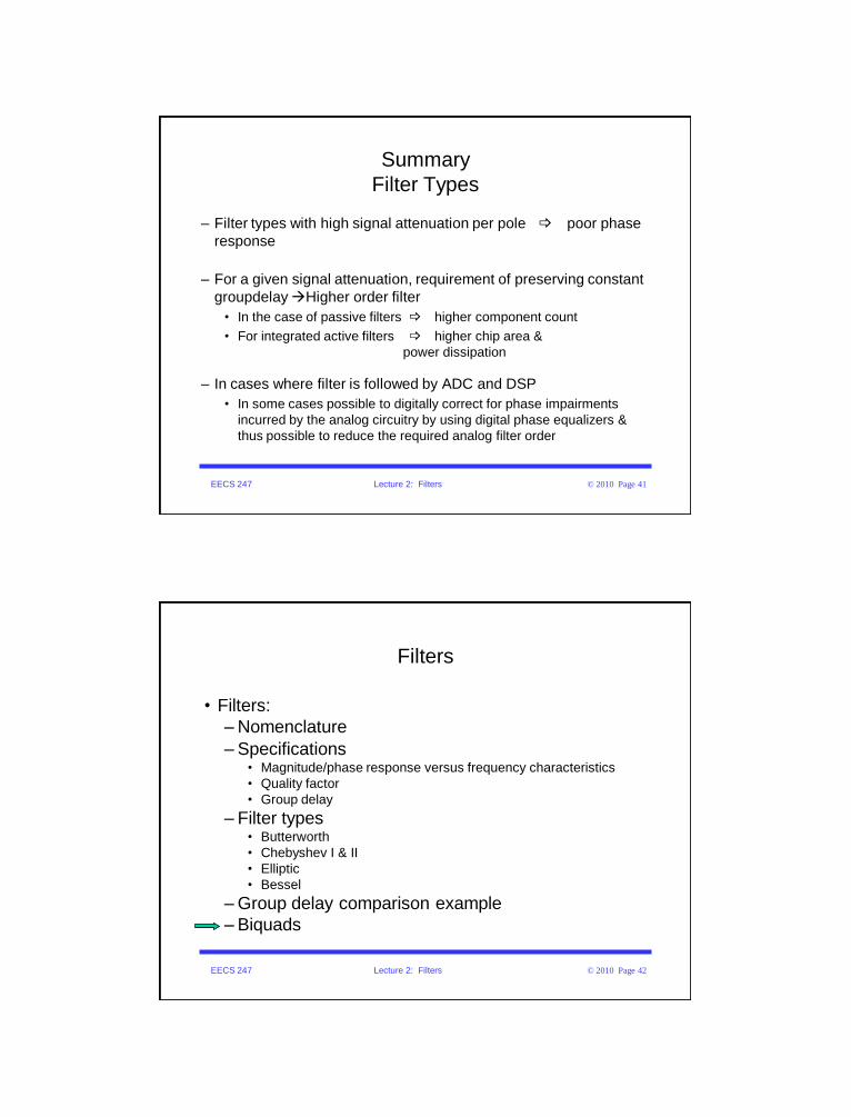
Summary
Filter Types
– Filter types with high signal attenuation per pole _ poor phase
response
– For a given signal attenuation, requirement of preserving constant
groupdelay Higher order filter
• In the case of passive filters _ higher component count
• For integrated active filters _ higher chip area &
power dissipation
– In cases where filter is followed by ADC and DSP
• In some cases possible to digitally correct for phase impairments
incurred by the analog circuitry by using digital phase equalizers &
thus possible to reduce the required analog filter order
EECS 247 Lecture 2: Filters © 2010 Page 42
Filters
• Filters:
– Nomenclature
– Specifications• Magnitude/phase response versus frequency characteristics
• Quality factor
• Group delay
– Filter types• Butterworth
• Chebyshev I & II
• Elliptic
• Bessel
– Group delay comparison example
– Biquads

EECS 247 Lecture 2: Filters © 2010 Page 43
RLC Filters
• Bandpass filter (2nd order):
Singularities: Pair of complex conjugate poles
Zeros @ f=0 & f=inf.
o
so RC
2 2in oQ
o
oo
VV s s
1 LC
RQ RCL
oVR
CLinV
j
s-Plane
EECS 247 Lecture 2: Filters © 2010 Page 44
RLC Filters
Example
• Design a bandpass filter with:
Center frequency of 1kHz
Filter quality factor of 20
• First assume the inductor is ideal
• Next consider the case where the inductor has series R
resulting in a finite inductor Q of 40
• What is the effect of finite inductor Q on the overall filter
Q?
oVR
CLinV

EECS 247 Lecture 2: Filters © 2010 Page 45
RLC Filters
Effect of Finite Component Q
idealfi l t ind.f i l t
1 1 1Q QQ
Qfilt.=20 (ideal L)
Qfilt. =13.3 (QL.=40)
Need to have component Q much higher
compared to desired filter Q
EECS 247 Lecture 2: Filters © 2010 Page 46
RLC Filters
Question:
Can RLC filters be integrated on-chip?
oVR
CLinV

EECS 247 Lecture 2: Filters © 2010 Page 47
Monolithic Spiral Inductors
Top View
EECS 247 Lecture 2: Filters © 2010 Page 48
Monolithic Inductors
Feasible Quality Factor & Value
Ref: “Radio Frequency Filters”, Lawrence Larson; Mead workshop presentation 1999
c Feasible monolithic inductor in CMOS tech. <10nH with Q <7
Typically, on-chip
inductors built as
spiral structures out
of metal/s layers
QL L/R)
QL measured at
frequencies of
operation ( >1GHz)

EECS 247 Lecture 2: Filters © 2010 Page 49
Integrated Filters
• Implementation of RLC filters in CMOS technologies requires on-chip inductors
– Integrated L<10nH with Q<10
– Combined with max. cap. 20pF
LC filters in the monolithic form feasible: freq>350MHz
(Learn more in EE242 & RF circuit courses)
• Analog/Digital interface circuitry require fully integrated filters with critical frequencies << 350MHz
• Hence:
c Need to build active filters without using inductors
EECS 247 Lecture 2: Filters © 2010 Page 50
Filters2nd Order Transfer Functions (Biquads)
• Biquadratic (2nd order) transfer function:
PQjH
jH
jH
P
)(
0)(
1)(0
2
2P P P
2 22
2P PP
P 2P
P
1P 2
1H( s )
s s1
Q
1H( j )
1Q
Biquad poles @: s 1 1 4Q2Q
Note: for Q poles are real , comple x otherwise

EECS 247 Lecture 2: Filters © 2010 Page 51
Biquad Complex Poles
Distance from origin in s-plane:
2
2
2
2 1412
P
P
P
P QQ
d
12
2
Complex conjugate poles:
s 1 4 12
P
PP
P
Q
j QQ
poles
j
d
S-plane
EECS 247 Lecture 2: Filters © 2010 Page 52
s-Plane
poles
j
P radius
P2Q- part real P
PQ2
1arccos
2s 1 4 12
PP
P
j QQ


