EE 2310 is a required course, prerequisite for EE 3320/3120

Erik Jonsson School of Engineering and Computer Science

The University of Texas at Dallas

© N. B. Dodge 12/13 1 Lecture #1: Introduction, History of Computing

EE 2310 • EE 2310 is a required course, prerequisite for EE 3320/3120. • Major topic areas:

– Binary and hexadecimal numbers – Combinational and sequential digital logic – Assembly language programming – Computer architecture overview

• EE 2310 Home Page: (http://www.utdallas.edu/~dodge/ee2310) – Syllabus, course information, lectures, announcements – Homework, work sheets, classroom exercise sheets – Review regularly!

• Note: Acrobat® Reader required. Obtain from Acrobat: http://www.adobe.com/products/acrobat/readstep2.html , or UTD software site: http://www.utdallas.edu/ir/local/index.html.



© N. B. Dodge 12/13

• Note that I do not use eLearning. • EE 2310 information is available on my website

(http://www.utdallas.edu/~dodge/ee2310 ). • Do NOT look for any course information on

eLearning. I grade and return tests 1 and 2 promptly, so you will NOT have to worry about your grade for long.

• (Test #3 is NOT returned.)

2 Lecture #1: Introduction, History of Computing

Note on 2310 Information



© N. B. Dodge 12/13

• There are three important EE 2310 documents: EE 2310 Syllabus, EE 2310 Homework Due Dates, and EE 2310 Lab Result Due Dates.

• The syllabus is very complete. It describes lectures, shows when tests and test reviews are scheduled, and lays out the semester schedule.

• Most course questions are answered in the syllabus or in the “due date” documents. The syllabus even has references to the texts used in the course.

• All three documents are on the 2310 website. 3 Lecture #1: Introduction, History of Computing

2310 Syllabus/Due Date Documents



© N. B. Dodge 12/13

• Read the syllabus carefully (preferably early this semester).

• Because 2310 documentation is so complete, here are questions that I really do NOT want to hear: – Is homework due today? Is there a lab due this week? – When is the next test? Do we have a worksheet today? – What should I be reading? What is the lecture about?

• Come to class prepared! – Class exercises printed. – Homework complete. – Lab report or results turned in.


Syllabus/Homework Due (Cont’d)



© N. B. Dodge 12/13

• At the top of the 2310 website is an announcements area.

• Important announcements will be listed there, either those made in class (e.g., about an upcoming test or assignment) or special items concerning a lecture or homework assignment.

• Sometimes office hours must be changed. These will also be noted in the announcements area.

• Scan the announcements section regularly!


Announcements on the Website



© N. B. Dodge 12/13

• There are three kinds of homework in EE 2310: – “Homework” – Homework is posted on the web site. Turn in at the

beginning of class on the due date (see due date schedule). Counts 10% of final grade. Answers posted on-line shortly after the due date.

– Note: The semester project is a homework assignment, but is a more difficult design assignment, that counts an additional 5% of your final grade. This assignment will be posted a little later in the semester.

– “Test Review Sheets” – Bring each completed review sheet to class the day of the test review. Will be checked by the instructor before class. TR problems are worked in class. Each TR is worth 1-point on your final grade (the +1 is a “completion grade”). Answers to test review sheets are NOT posted! You must come to class for the answers.

– Lab Report/results. Due according to the lab result due date sheet. Worth 10% of your final grade. More on labs below.


Homework



© N. B. Dodge 12/13

• All homework (including lab reports) will be turned at the beginning of EE 2310 class on the due date listed, except for the items noted below.

• Software lab results (programs in labs 5 and 6) and programs in Homework #’s 6 & 7 will be emailed as an attachment directly to the class TA. Each student turns in homeworks 6 & 7.

• The TA’s schedule, availability, and office location will be listed on the EE 2310 web site as soon as TA’s are assigned.

• In the case of labs 5 and 6, only one program is required per team. • Make sure you list both partner’s names on each lab report and

program, so that proper credit is given to both lab partners! • Both partners submit the semester project independently,

although they may work on it together. 7 Lecture #1: Introduction, History of Computing

Homework Procedures



© N. B. Dodge 12/13

• Print out and bring (real paper!) class exercise sheets to class. They are included in the lecture notes, which you can read prior to the class if you wish.

• Selected exercise sheets will be collected to earn points on your next test (+1-3 per sheet; up to 5 points total).

• You will not know in advance which in-class exercises will be turned in, or which worksheets will be checked.

• Certain class exercise sheets will not be completed in class, but will be assigned as a bonus homework. Bonus exercise sheets should be turned in at the start of the next office hours (similar bonus points apply).


Class Exercise Sheets



© N. B. Dodge 12/13

• There are six lab exercises in EE 2310. • The lab portion consists of four digital hardware

exercises which are to be completed in the EE 1202/2310 lab. You will work with a lab partner, and the partnership will submit a joint report summarizing the exercise and their results.

• There are also two software assignments that count as labs, but no report is required. Simply work with your partner to complete the software design assignment, and email your result to the class TA.

• Labs count 10% of your final grade. 9 Lecture #1: Introduction, History of Computing

EE 2310 Labs



© N. B. Dodge 12/13

EE 1202/2310 Lab Facility Overview

• The EE 1202/2310 lab is ECSS 4.622 (“new” engineering building), on the third floor of the ECSS building.

• As noted above, lab exercises will be done by teams of two students, working together. You can choose your own lab partner. If you do not have a partner, come to the instructor and he will find you one.

• You will do these labs on your own, at your own rate. • There are no scheduled lab times. Go to the lab and do

your lab work when you wish (subject to lab open hours).




© N. B. Dodge 12/13

Lab Hours • ECSS 4.622 is open ten hours a day, 10 AM to 8 PM,

four days a week, Monday-Thursday. • You are free to work on your lab at any time during

these hours. You can do the lab all at once, or do a part of it and come back and do the rest later.

• There are 12 workstations in the lab. You must sign up to reserve a workstation. Workstations may be reserved in two-hour slots, M-R.

• If you come to the lab and a station is free, you may start work immediately. Remember to put your name on the reservation chart for that current period!




© N. B. Dodge 12/13

Reservation Sheets • Each week, reservation sheets for the

next week be available in the lab at 10 AM Thursday morning.

• You must reserve a lab station (you can “drop in” and start immediately if a station is free). Write your name in the reservation block. Include the course number, since EE 1202 and EE 2310 both use this lab.

• You can reserve no more than four hours per week, either in different 2-hour slots or contiguously.

• Please be prompt. If you are 15 minutes or more late, your reservation is voided.

• Reservations for the week may be made from the previous Thursday through the rest of the next week.


Time Slot Reserved Workstation 10 AM 12 Noon 2 PM 4PM 6 PM

1

2

3

4

5

6

7

8

9

10

11

12



© N. B. Dodge 12/13

ECSS 4.622 Lab

• The entrance to 4.622 is shown on the right.

• There are twelve workstations in the lab room.

• Workstations have a number of instruments, but you will only use the IDL-800 digital prototyping unit and possibly the PC.

• Instruments leads are on hangars at the front of the lab, although you will probably not need these.

Lecture #1: Introduction, History of Computing 13



© N. B. Dodge 12/13

Lab Cabinets • ECSS 4.622 is used for two sets of

laboratory exercises, those in EE 1202 and those in EE 2310.

• As shown in the picture to the right, there are three cabinets inside the 4.622 door, to your immediate left.

• One cabinet contains EE 2310 parts. • The second contain EE 1202

experimental parts. • The third is a general-purpose cabinet

for both labs, containing miscellaneous support material required for both labs.

• If any EE 2310 material is not in the 2310 cabinet, it is in the “misc” cabinet.




© N. B. Dodge 12/13

Layout of 2310 Cabinet

• The contents of the 2310 cabinet are shown to right.

• Note the layout of the cabinet to be sure that you can quickly get required components and get to work.




© N. B. Dodge 12/13

Layout of Miscellaneous Cabinet

• The Miscellaneous cabinet contains many items that will not be used regularly.

• Items such as the first aid kit are available in case of minor injuries (unlikely in EE 2310, but possible).

• Check items in this cabinet when you first go into the lab to make sure you know the various items that are available.




© N. B. Dodge 12/13

Digital Parts Kits

• These kits are mainly for EE 2310, although they are used for one EE 1202 experiment.

• They contain the digital circuits, (“ic’s”) also arranged in partitions in groups of digital circuits.

• Circuit parts needed for each lab exercise are identified on the last page of the exercise.

• You can select ic’s from the kit by their part numbers.




© N. B. Dodge 12/13

Wiring Kits

• Wiring kits are used to connect digital circuits together for each experiment.

• The wires are various lengths, made of multi-strand copper, with hardened tips to plug into the circuit boards.

• Please be certain that the wires are returned to the kits and properly arrange in the various kit partitions.




© N. B. Dodge 12/13

Bench Layout • The layout of the bench

instruments is shown to the right.

• The items as shown to the right are: – Power supply – Digital multimeter – Signal generator – Oscilloscope – Digital prototyper – LC meter (stations 5, 12)




© N. B. Dodge 12/13

Instrument Identification

Instrument identification: A – Power supply B – Digital multimeter C – Signal generator D – Oscilloscope E – Digital prototyper (only instrument used in EE 2310) F – LC meter (stations 5, 12)


•A

•B •C •E •D •F



© N. B. Dodge 12/13

Lead Hangers

• Leads are stored on the hangars at the front of the lab as shown in the picture to the left (leads also on the other side of the cabinet).

• You will probably not need these in EE 2310 – they are mainly for use in EE 1202.




© N. B. Dodge 12/13

Lab Layout


Comm

Cabinet

Workstation

8 Workstation

3

Cab

inet

Workstation

7 Workstation

4

Workstation

6 Workstation

5

Cab

inet

Workstation

9 Workstation

10 Workstation

12 Workstation

11

•File •Cabinet

Cab

inet

Workstation

2 Workstation

1 EE 2310 Cabinet

Misc. Cabinet

EE 1202 Cabinet

TA T

able

•Door



© N. B. Dodge 12/13

Lab Report Due Cycle

• Lab assignments are due per dates in the due date chart (generally two weeks after assigned).

• Late lab reports are generally NOT accepted. Exceptions can be made for very severe problems (such as your death).

• For the two software lab assignments, no reports are required. Simply complete the assignment jointly with your partner and turn in on the assigned date. The method of submission is to email the assembly language program as an attachment to the class TA. Lecture #1: Introduction, History of Computing 23



© N. B. Dodge 12/13

Lab Routine 1. Read your lab exercise in the text before the briefing. 2. Reserve your lab space (can do on previous Thursday). 3. Go to the lab at your reserved time and get out a parts kit.

Do the lab exercise at your reserved station. 4. When finished, have the lab TA initial your results, put

away parts and equipment and make sure that your workstation is clean. The lab TA will check your station.

5. Each team submits one lab report, turned in to the EE 2310 class TA (his/her information will be posted on the 2310 website). Make sure to follow report guidelines as posted on-line. Lab reports only on labs 1-4.

6. Submit programs (labs 5 and 6), as discussed above, by email – no lab reports for these labs.




© N. B. Dodge 12/13

• Turn off your cell phone. • Please close and put away your laptop. DO NOT

use your laptop in class (except as directed). • Please pay attention and perhaps take a few brief

notes. EE 2310 material is tough – and it is easier than most courses to come!

• Bring required materials to class (test review sheets and class exercise sheets). These are worth points on tests or on your final grade.


Lecture Ground Rules




Purpose of EE 2310

• EE 2310 lays the foundation for an understanding of computer architecture (that is, the way computers are put together, the identity and characteristics of their component parts, and their basic instruction sets).

Digital Devices

Digital Circuits

Computing Circuits

Computer Architectures and Designs

Instruction Architecture and Design

Assembly Language

Assembly Language Programming




What is a Computer?

• Computer: A collection of electronic switches that can perform mathematical and logical calculations.

• It can be programmed to solve problems by loading instructions which the computer can execute.

• Computer components – circuits, chasses, peripherals – are called hardware.

• Computer programming instructions are called software. • Most computers have common hardware components:

– CPU’s (central processors, 1 or more) – performs calculations – Data and instruction memory (called “RAM” or DRAM”) – Permanent storage memory (“hard drive” or CD-ROM) – Input/control devices (keyboard, mouse, CD/DVD) – Information output devices (LCD display, printer, CD/DVD)




History of the Computer

• Although mathematical computation devices go back into the middle ages (e.g., the abacus), modern electronic computers have a relatively short history.

• This history is one of the most remarkable stories of technological innovation in the history of mankind, made possible by the invention of the transistor in the 1940’s.

• What follows is a brief history of the electronic computer since its invention only a few decades ago (although we start with a few antecedents of the electronic digital computer).




History of the Electronic Computer • In the beginning, there were only a very few computers, and

they were VERY, VERY LARGE. – First mechanical (cams and levers), early 1900’s-1940’s. – Then large, HOT vacuum tubes (a picture later), 1940’s-1950’s. – “Computers in the future may have only 1,000 vacuum tubes and

perhaps only weigh 1½ tons.”—Popular Mechanics (1949). • In the intervening years, things have changed…

– “… the cost of computing has fallen 10 million-fold since the microprocessor was invented in 1971. That’s the equivalent of getting a Boeing 747 for the price of a pizza. If this innovation had been applied to automotive technology, a new car would cost about $2; it would travel at the speed of sound; and it would go 600 miles on a thimble of gas.”—Bob Herbold, COO of Microsoft, in “letter to Ralph Nader” (11/13/97)

Quotations courtesy C. Cantrell




The Need for Computers Drove Development

• Scientific Needs: – Accurate math tables,

complex scientific calculations

• Business automation: – Payroll, accounting

• Government needs: – Census tabulation, employee

records, tax files (!) • Military requirements:

– Artillery tables, decryption, nuclear weapon design

Artillery Calculator

Eniwetok Atoll, 1952




The First Computers • Scientists begin to design “calculating

machines” in the 1800’s. • Charles Babbage (1791-1871)

designed the first complex “mechanical computer” in 1834.

• He and colleagues attempted to build a steam-powered model with £20,000 funding from the British government.

• The machine was never finished (due to limitations of mid-19th century technology), but a copy built in the 1990’s actually worked!

• It was the work of mathematician George Boole, later in the 19th century, that would lead the way for modern computing.

Reproduction of the Babbage Difference Engine built in the early 1990’s.




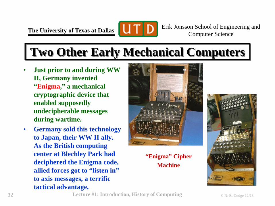
Two Other Early Mechanical Computers • Just prior to and during WW

II, Germany invented “Enigma,” a mechanical cryptographic device that enabled supposedly undecipherable messages during wartime.

• Germany sold this technology to Japan, their WW II ally. As the British computing center at Blechley Park had deciphered the Enigma code, allied forces got to “listen in” to axis messages, a terrific tactical advantage.

“Enigma” Cipher Machine



© N. B. Dodge 12/13

Two Other Early Mechanical Computers (2)

• Also prior to WW II, the mechanical punched-card sorter was invented, enabling the automatic sorting of large amounts of data.

• IBM entered the computing business making these sorters.

33 Lecture #1: Introduction, History of Computing, Binary Numbers

Hollerith Card Sorter




The First Electrical Computers

• One of the first computers powered by electricity was the Harvard Mark II, which used direct-current electrical relays to do all its calculations.

• Such a relay is shown above.

Computer Relay




The First Computer “Bug” • The term “computer bug” was

born when a small moth flew into one of the Mark II cabinets and stuck a relay open.

• Searching for why the computer had ceased operation, a young female computer scientist, Grace Hopper, discovered the “Bug.”

• The page shown is reputed to be in the Smithsonian Museum.

• Grace Hopper was a career Naval Officer and retired as an Admiral (she also invented COBOL).

The First Computer “Bug”

Grace Hopper as a Young Naval Officer (and Computer

Scientist)

Rear Admiral Grace Hopper




The First Electronic Computers

• After the advent of electrical computers using relay switches, designers began to incorporate vacuum tubes, which were becoming readily available due to their use in radios.

• An early computer was ENIAC, a monster that weighed 30 tons and was designed to calculate artillery ballistics tables.

• John Mauchly and J. Presper Eckert, who designed it (with help from many others) are generally accorded the title of “designers of the first computer.”

• History has pretty well ignored women’s contribution to the development of this first computer (and computing in general).

• In fact, a group of women were the first programmers on the ENIAC. In those days (circa 1943-44), programming was a really hard task, since there was NO software (and no manuals!).

• These talented young women take their place beside Grace Hopper as some of our most important computer pioneers.




The First Programmers • “Programming” the ENIAC

meant physically configuring the computer processing elements to do the calculating task.

• This involved not software, but switches, plug panels, and a thorough knowledge of the hardware.

• Shown at right is one of these first programmers.

• Women were major players in computing technology from the start. Courtesy IEEE Spectrum




Vacuum Tube Computer Elements

• To the right is a typical vacuum tube computer circuit.

• This circuit (about as big and complicated as the entire electronic assembly of a modern PC) was only one tiny part of a vacuum tube computer.

• As noted earlier, vacuum tube computers typically weighed many tons. Courtesy University of Virginia Computer Department




Second-Generation Electronic Computers

• The second generation of digital computers were developed in the early 1960’s using transistors, invented in the late 1940’s and now beginning to be available commercially.

• One such computer was the Burroughs B5000 series, developed about 40 years ago.

• An early transistor circuit is shown as well.

Both figures courtesy of University of Virginia Computer Department




Early Integrated Circuit Computers

• The third generation of electronic computers were the first built with “integrated circuits,” solid-state circuits with multiple transistors (and other circuit elements) on the same chip of silicon.

• The computer shown above is the Control Data Corporation Model 7600, one of the first computers built with integrated circuits and also one of the first scientific “super computers” (cost: > $5 million!).




“Fourth-Generation” Electronic Computers

• The next generation of electronic computers featured “VLSI” integrated circuits (circuits with many transistors per chip).

• Computer processors still consisted of many custom VLSI modules on multiple printed circuit boards.

• Computers of this era included: – General-purpose computers such

as the IBM 3xxx, 43xx series. – The first minicomputers, such as

the Digital Equipment VAX 8400, PDP 11, the Data General Nova, and the Honeywell 516.

– Supercomputers such as the Cray-2, Cray X-MP.

The Cray X-MP. Cray computers were the premier supercomputers in the 1980’s. Cray Computer was founded by Seymour Cray, a former Control Data employee, who quit CDC and started his own company because he thought that CDC was moving too slowly in bringing out new models.




Computer Memory

• Early memories were exotic: Magnetic drums, columns of liquid mercury (!).

• In the 1950’s, magnetic “core memory” became the standard for “working” data memory. Data was stored by magnetizing tiny donuts of magnetic material.

• Electronic memory (or “DRAM”) brought about the era of cheap computer memory in the 1970’s.

• Magnetic disks remain a primary method of bulk data storage due to their very low (and constantly decreasing) cost.

Computer Core Memory.

Intel 1K DRAM




“Computers on a Chip” – Generation 5

• Starting in the mid-late 1970’s, computer processors on a chip and large electronic memories became available.

• This led to the first affordable personal computers (Altair, Apple I, Osborne I, and the IBM PC).

• Single-chip processors included the Intel 4004, 8008, 8086, 80286 and 80386 and the Motorola 6800 and 68000.

• Later single-chip computers included the Sun SPARC (made by TI), the Digital Equipment Alpha, the Motorola PowerPC and 88000 (as well as the 68010-68040) and the Intel Pentium, Pentium II, III, and IV.




One of the Chips That Started It All • Intel 4004 (introduced November

1971). • Clock speed: 108 KHz (yes, that’s

right, 108,000 Hz). • ~2300 transistors (!). • 10 μ feature size (1 μ = 10−6 m). • Used initially in some of the first

small, portable calculators that were produced.

• Also used to provide “imbedded intelligence” in some early computer-controlled devices.

• Notice 16 output wires/pads.




“State of the Art”

• Intel Core i7 Extreme Processor*, (6 processors on chip), ~130+ Watts.

• Features: 4.0 GHz clock (4.2 O/C), 15M Cache, up to 1866 MHz FSB.

• Currently built with the 22 nanometer (“Haswell”) process (22 nanometers = 0.022 microns, less than 0.4% of the minimum feature size of the Intel 4004!). * Aug., 2014



© N. B. Dodge 12/13

“State of the Art”

• Intel Xeon E5-2697, 130 Watts.

• 12 cores, 2.7 GHz. • 30 MB cache. • Also 22 nm lithography. • ~$ 2500. • Aimed at high performance

workstation and blade market.




© N. B. Dodge 12/13

• Four compute cores, 8 graphics cores.

• Up to 4 GHz, can be overclocked. ~ 100W.

• Lithography not clear, probably 22 nm.

• Said to be aimed at gaming applications.


AMD A10-7850K




Generation 6 – Embedded Processors

• Today, computers are not only an invaluable tool for almost everyone (e.g., the personal computer), they are also embedded in just about any device and appliance that one can imagine: – Every mobile telephone has a computer in it. – Many appliances have embedded computers (washers, dryers,

televisions, cable boxes, computer printers, DVD players/ recorders, microwave [and regular] ovens, etc).

– We are even beginning to see “smart clothing” – apparel that has embedded computing as a part of the material.




Smart Clothing • An example of embedded processing is

the Adidas 1. • Introduced in 2005, it features “active

cushioning.” A processor in each shoe constantly measures sole forces as the user runs, then activates a motor, which shortens or lengthens a cable attached to a cushioning element.

• The cushion is compressed or relaxed by the cable, making it softer or firmer depending on the need of the runner.

• Cost $250 at introduction in 2005, discontinued in 2006-7. Still available from some sources for $100-150.

http://www.skuAddToC