Embed Size (px)
Citation preview

ECONOMICS
THE EFFECTS OF MACROECONOMIC SHOCKS ON THE DISTRIBUTION OF PROVINCIAL OUTPUT IN CHINA: ESTIMATES FROM A RESTRICTED VAR
MODEL
by
Anping Chen, School of Economics,
Jinan University, China
and
Nicolaas Groenewold Business School
University of Western Australia
DISCUSSION PAPER 14.13
THE EFFECTS OF MACROECONOMIC SHOCKS ON THE DISTRIBUTION OF
PROVINCIAL OUTPUT IN CHINA: ESTIMATES FROM A RESTRICTED VAR MODEL
by Anping Chen,
School of Economics, Jinan University,
Guangzhou, China
and
Nicolaas Groenewold,* Economics Programme,
UWA Business School, M251, University of Western Australia,
Perth, Australia
DISCUSSION PAPER 14.13
*Corresponding author.
This paper has benefitted from comments received at the joint CESA-JNU International Conference
on Industrial Upgrading and Sustainable Economic Growth in China, Jinan University in December,
2013, the 3rd International Workshop on Regional, Urban, and Spatial Economics in China, Fudan
University, Shanghai in June 2014, the ACE/ESAM conference in Hobart in July 2014, the annual
CESA conference held at Monash University in July 2014 and, particularly, at an Economics Work-
in-Progress Workshop at UWA in May 2014. This research was partially funded by a National
Natural Science Foundation of China Grant (No. 71173092) and the Program for New Century
Excellent Talents in University, Ministry of Education of China (No. NCET-12-0681).

ABSTRACT
The extent and persistence of the inequality of the inter-regional distribution of output is an
important policy issue in China and its sources have been the subject of considerable
empirical research. Yet we have relatively little empirical knowledge of the effects on the
regional distribution of output of shocks to national macroeconomic variables such as GDP
and investment. This is an important gap in the empirical literature since much government
macroeconomic policy seeks to influence GDP using instruments such as investment
expenditure. It is likely that such national shocks will have differential regional impacts and
so affect the regional output distribution. Policy-makers need to know the sign, size and
timing of such effects before making policy decisions at the national level. We simulate the
effects of aggregate shocks on individual provinces’ GDP within the framework of a vector
autoregressive (VAR) model restricted in a manner following Lastrapes (Economics Letters,
2005). We use annual data from 1953 to 2012 to estimate the model which includes 28 of
China’s provinces and simulate the effects on provincial outputs of shocks to aggregate
output and investment. We find great diversity of effects across the provinces with
discernible geographic patterns. We also observe variability across the effects of different
aggregate shocks.
Keywords: regional output distribution, economic growth, China
JEL categories: E61, R50, O53

1. Introduction
Although China has steadily climbed up the world league-table in terms of GDP per
capita since opening-up and reforms began to take hold in the 1980s, there have been
substantial and persistent problems with the distribution of this growing output.1 Of course,
this tension between growth and the distribution of the fruits of growth is not new, nor is it
restricted to China. A recent United Nations report (United Nations, 2013) argues that
inequality is widespread, multifaceted and persistent.
In this paper we focus on the regional distribution of GDP in China, taking the
provinces as the regions. The distribution of GDP per capita has fluctuated over the period
since the beginning of reforms, with the coefficient of variation falling steadily over two
decades from the late 1970s until the late 1990s, when it began to rise so that by 2004 it had
returned to the level of the mid-1980s, after which it declined steadily to the end of the
decade.2 Despite recent declines in inter-regional inequality, the ratio of GDP per capita in
the richest province in 2012 (Jiangsu) to that of the poorest (Guizhou) was still 3.5, a very
large disparity by any standards.3
The uneven regional distribution of output has been a perennial policy issue at the
highest levels of Chinese policy-making since the inception of the People’s Republic of
China, with disproportionately large allocations of investment to the interior region occurring
during much of Mao Zedong’s rule in an attempt to redress the balance of output in favour of
the poorer inland provinces. Subsequent to the beginning of reforms under Deng Xiaoping,
allocation of resources swung towards the coast on the basis of the argument that investment
1 China’s ranking on the basis of GNI per capita in World Bank tables rose from 130th in 1990 to 120th in 2000 and 77th in 2012. See http://data.worldbank.org/indicator/NY.GNP.PCAP.CD, accessed 24 October, 2013. 2 This characterisation is based on the coefficient of variation for nominal provincial GDP from 1978 to 2012. The source of the data is described in the data section below. 3 The question of exactly whether, and, if so, how and when regional economies in China have been converging has been the subject of a great deal of empirical research. To survey this would take us too far afield in this introduction but see Groenewold et al. (2008) Chapter 2 and the interesting recent contribution by Andersson et al. (2013) and references there.
1

was likely to be most productive there and that, eventually, the growing coast would drag the
rest of the country with it to general prosperity and smaller disparities. By and large, the
latter has not happened and since the 1990s policy-makers increasingly re-focussed on the
problems of large and persistent differences in per capita GDP across the provinces.4
Policies to ensure a more equal distribution of output are clearly desirable on the basis
of equity and have also been supported on the basis of the danger of social unrest which
might be caused by widening gaps between rich and poor regions. Yet, there has been a
noticeable caution in the vigour with which such policies are pursued by policy makers who
are reluctant to jeopardise the continuation of a high aggregate growth rate. This has been
particularly true in light of the recent growth slowdown following the Global Financial Crisis
and the ensuing slower growth rates in most of the OECD.
There is, in some quarters at least, a perception that directing policy to reduce regional
inequality may have a cost in terms of lower national performance, a perception not restricted
to policy-makers but also evident in the research literature. Thus, e.g., Wong (2006) asserts
that inequality is an inevitable consequence of growth policy in China and only its severity is
surprising. Similarly, Knight (2008), argues that income inequality is unavoidable, at least in
the early stages of development. Further, Zhu and Wan (2012) find a trade-off between
growth and equality and argue that if China is to foster a balanced and harmonious economy,
there must be a shift in focus from growth to equality.
Of course, those familiar with the literature on economic development and on regional
development in particular, will realise that the consideration of such a trade-off is not new.
Indeed, it dates back at least to the work on the inverted-U curve between economic
development and inequality; see particularly Williamson (1965) and earlier work by Kuznets
(1955), Myrdal (1957) and Hirschman (1958). The idea captured by the inverted-U curve is
4 See Groenewold et al. (2008), Chapter 3 for more information on Chinese regional policy since the founding of the People’s Republic of China.
2

that in the early stages of development regional (and other) inequality rises but eventually
falls as development (usually measured in terms of income or output per capita) proceeds.
There is thus a systematic relationship between inequality and development which has an
inverted-U shape.
A substantial theoretical and empirical literature has developed in the area of growth
and inequality but little consensus has been reached. Thus theoretical analysis in papers by
Galor and Zeira (1993), Alesina and Rodrik (1994), Persson and Tabellini (1994) and
Benhabib and Rustichini (1996) present arguments that growth and inequality are negatively
related while Kaldor (1956), Benabou (1996), Edin and Topel (1997) argue the opposite.
Empirical work is equally inconclusive with the work reported in papers by Alesina and
Rodrik (1994) and Persson and Tabellini (1994) finding that inequality is harmful for growth
while Forbes (2000) reports the opposite finding and various papers present ambiguous
results including those by Barro (2000), Partridge (2005), Fallah and Partridge(2007),
Chambers (2007), Bjornskov (2008) and Barro (2008).
The literature on inequality and development in China is relatively sparse. Kuijs and
Wang (2005) argue that China can have a more balanced growth path with a sustainable
reduction of income inequality if appropriate policies, such as reducing subsidies to industry
and investment, encouraging the development of the services industry and reducing the
barriers to labour mobility are implemented. Wan et al. (2006) explicitly tested the growth-
inequality nexus in China, focusing on rural-urban income inequality and regional growth
using a provincial-level panel data set. They found that an increase in inequality has negative
effects on growth, irrespective of time horizons so that reductions in inequality will be
growth-enhancing. Qiao et al. (2008) find the opposite: fiscal decentralisation has resulted in
more rapid economic growth accompanied by greater regional inequality. In a more recent
test of the possible growth cost of reducing regional inequality, Chen (2010) tested the
3

relationship between growth in per capita GDP and the Gini coefficient as a measure of inter-
regional inequality in a multivariate time-series model and found that a reduction in
inequality comes at the cost of growth in the short run but not in the long run. On the basis of
a mixture of theoretical and empirical analysis, Zheng and Kuroda (2013) argue that whether
there is a trade-off between growth and regional equality depends on the driver of growth – if
growth is driven by transportation infrastructure expenditure, it comes at the cost of increased
inequality while the opposite is true if growth is generated by investment in knowledge
infrastructure.
To sum up, there is a substantial literature, both theoretical and empirical, in the
broadly-defined area of inequality and development but no consensus on the sign of the
relationship between them. Moreover, there are relatively few papers which deal explicitly
with China and the findings of such work as there is are contradictory.
In the work reported in this paper we contribute to the empirical literature on China
by focussing on the provincial distribution of output (rather than a single inequality measure)
and for this we use a novel empirical approach which allows us to analyse how a change in
national growth is distributed across the provinces. We go on to investigate whether the
source of the growth matters by explicitly adding aggregate investment to the model.
The method we use is based on a restricted VAR model developed and used by
Lastrapes (2005, 2006) to analyse the relationship between changes in the aggregate inflation
rate and the dispersion of individual prices. Applying this to the regional growth context
allows us to trace through the effects of a change in an aggregate variable such as the growth
rate on the per capita GDP of all provinces rather than on a single summary measure of the
distribution such as the coefficient of variation or the Gini coefficient, which has been a
characteristic of most existing empirical work.
4

We find that aggregate multipliers for both output and investment shocks are plausible,
with the effect of a boost to investment being larger than that of a general output shock.
At the provincial level, we find great diversity in the geographical distribution of the
effects of aggregate shocks – in most cases approximately half the provinces have responses
significantly different to the national average. For the main sample period (1980-2012), we
find that the above-average responses to an output shock are concentrated in the coastal
provinces and a few central provinces. The effects of an investment shock are more diffused
with the above-average effects covering much of the north-east and central regions. There is
some statistical evidence that the effects of an investment shock are biased in favour of the
poorer provinces
Cross-section regressions showed that, in the case of an investment shock, there was
significant evidence that provinces which were poor at the beginning of the sample tended to
benefit more than the rich – consistent with a “bias-to-the-poor” approach of the central
government investment allocation policy. No such result was detected for an output shock.
The remainder of the paper is structured as follows. In section 2 we set out the
empirical model based on the work of Lastrapes. The data to be used are described in section
3. The results for the base model are discussed in section 4, with extensions and robustness
tests reported in section 5. Conclusions are drawn in the final section.
2. The empirical model
As observed in the previous section, existing empirical literature which examines
the effect of growth shocks on regional distributions typically uses a summary measure of the
distribution such as the Gini coefficient or the coefficient of variation calculated from the
cross-section of regional GDP per capita values. This makes the analysis tractable but loses
much of the information about the distribution across regions as well as information on the
5

response of individual regions to aggregate shocks. An alternative approach is to estimate
and simulate a model which includes the aggregate variables such as the national growth rate
as well as all the regional per capita GDP variables. This is possible if there are relatively
few regions so that there are sufficient degrees of freedom given the size of the data sample.
Where this is not the case, the estimation of such a model becomes intractable unless
restrictions are imposed to reduce the number of parameters which must be estimated.
There are various ways in which the system can be restricted to achieve tractability.
One is to reduce the number of regions into a few large ones, on the assumption that the
components of the larger region are homogeneous – see, e.g., Carlino and DeFina (1998).
Another approach is to estimate a set of linked VAR models, one for each region.
Alternatives are a GVAR structure (see, e.g., Pesaran et al., 2004), and one which includes
aggregate variables as well as some summary measure of the remaining regions such as
carried out by Carlino and DeFina (1999) and, more recently, by Owyang and Zubairy (2013).
The disadvantage of the use of a few large regions is that detail on regional disaggregation is
lost while the second set of alternatives generally suffers from the drawback that the
aggregate shocks are not constrained to be the same across the regions since each regional
VAR model is used to identify its own aggregate shocks.
Lastrapes (2005) proposed a set of restrictions which overcomes both of these
disadvantages. Essentially, he restricted the interaction both between the aggregate variables
and the regional variables as well as amongst the regional variables themselves. The approach
was used in Lastrapes (2006) in the analysis of the effects of aggregate inflation shocks on
the distribution of individual prices. Subsequent applications of the method include
Beckworth (2010) and Fraser et al (2012), both of whom applied it to problems where the
disaggregated variables had a regional dimension; indeed, both analysed the issue of whether
6

aggregate monetary shocks have uniform effects across regions – the states of the US in
Beckworth’s case and the states of Australia in the application by Fraser et al.
We wish to analyse the effects of aggregate macroeconomic shocks on individual
provincial GDPs in China. With 31 provinces and annual GDP data for (at most) 60 years,
estimation of a VAR would run into degrees-of-freedom problems very quickly so that the
Lastrapes procedure seems ideally suited to this application.
The Lastrapes approach can be developed as follows. Consider a vector of variables,
zt which includes both national and regional variables. Partition zt into two parts,
(1) zt = (z1t, z2t)’
where the first component consists of the regional variables (regional per capita GDPs in our
case) and the second consists of the national variables. It is expected that there are many
regional variables and few national variables. Assume that the elements of zt are related by a
linear structural dynamic model of the form:
(2) A0zt = A1zt-1+…+Apzt-p+ut = A(L)zt+ut
where A(L) is a polynomial in the lag operator, L, A(L) = A1L+…+ApLp and the error process
satisfies E(ut) = 0 and E(utut’) = I, the identity matrix. Thus the errors in the structural model
(the structural errors) are assumed mutually uncorrelated and the equations of the model are
normalised so as to ensure a unit variance for each error.
There are two difficulties in using the model as it stands. The first is that it is not
identified – all the equations in (2) have the same variables. This is a standard problem with
structural models of this type and requires additional restrictions to be placed on the model,
the most common of which are short-run Bernanke-Sims restrictions (including those based
on the Cholesky decomposition of the covariance matrix of the errors) and the long-run
7

Blanchard-Quah restrictions.5 In either case the model is first transformed into a reduced-
form one by pre-multiplying by the inverse of the matrix A0 to obtain:
(3) zt = A0-1A(L)zt + A0
-1ut ≡ B(L)zt+εt
where B(L) ≡ A0-1A(L) and εt ≡A0
-1ut. The reduced-form model can be estimated by OLS
and the restrictions used to identify the elements of the A0 matrix which can then be used to
retrieve the structural parameters and errors from their reduced-form counterparts. The
retrieval of the structural errors is important since the reduced-form errors will be correlated
with each other (each is a linear combination of all the same structural errors), making it
illegitimate to shock them independently. The structural errors are, by assumption,
uncorrelated and therefore can be shocked independently.
The second difficulty likely to be faced in the estimation of model (2) is a degrees-of-
freedom problem that arises if there are many regional variables relative to the number of
observations in the sample period. Lastrapes (2005) developed a method for overcoming this
problem in a model in which there was a small number of aggregate variables (national
variables in our case) and a large number of disaggregated variables (regional variables in our
application). He proposed two assumptions: (i) the aggregate variables are block exogenous,
and (ii) the disaggregated variables are mutually independent once they have been
conditioned on the aggregate variables. The first of these assumptions implies that the
disaggregated variables do not jointly (Granger-) cause any of the aggregate variables and the
second implies that the disaggregated variables are mutually correlated only insofar as they
are related to common aggregate variables. Under these assumptions, Lastrapes showed that
the model could be written as two components, one a standard VAR in the aggregate
variables and the other a series of individual equations for the disaggregated variables. In
particular:
5 See Enders (2010) for a textbook treatment of these issues.
8

(4a) i
p pi
t1t 11 1t -i 2t -ii=1 i=1
z = B z + G z +v
(4b) p
i2t 22 2t -i 2t
i=1z = B z + ε
The equations in (4b) are simply a standard VAR in the aggregate variables and can
legitimately be estimated by OLS. Since we are interested in shocking the errors in the
equations only for the aggregate variables, identification of the structural errors is necessary
only for the VAR in (4b) and can be based on commonly used restrictions for VARs
mentioned earlier. Lastrapes shows that the matrix i11B in equation (4a) is diagonal so that
each of the equations for the disaggregated variables has only lags of the dependent variable
and current and lagged values of the aggregate variables as regressors. The assumption of the
block exogeneity of the aggregate variables ensures that there is no contemporaneous
correlation between the regressors and the errors terms in the equations. In addition
Lastrapes shows that the covariance matrix of the errors in (4a) is diagonal so that there is no
gain to be had from estimating the equations simultaneously by the Seemingly Unrelated
Regressors Estimator. Hence, the equations in (4a) can legitimately be estimated one-by-one
using OLS.
In our application, the aggregate variables will be national GDP and investment and
the disaggregated variables will be provincial GDPs. In this paper we will use the Cholesky
scheme for identifying the structural errors in the VAR part of the model. We assess the
robustness of our results by including a wider range of aggregate variables as well as by
experimenting with the Bernanke-Sims identification procedure for the aggregate VAR
component of the model.
9

3. The data
We require data for two types of variables: national and regional. With one exception,
all data are annual from 1953 to 2012.6
The regional variables are real provincial GDP which we use in log per capita terms.
The data are taken from Wu (2004) and various issues of the China Statistical Yearbook and
are in terms of yuan per capita in 1953 prices. We use data for 28 of China’s 31 provinces
(including the “city-provinces” of Beijing, Shanghai and Tianjin) with Chongqing included in
Sichuan, Hainan included in Guangdong and Tibet excluded, all for reasons of missing data.
Two national variables were used in the main analysis: real GDP and real investment
in fixed assets. Additional variables used in the robustness tests are consumption expenditure,
government expenditure, merchandise exports and imports and world GDP. All are in real
per capita terms and, except for the world GDP, all variables are in yuan at 1953 prices and
taken from New China 60 Years Statistics Compilation (National Statistical Bureau, 2009)
and China Statistical Yearbook (National Statistical Bureau, various issues). Population data
used to compute per capita magnitudes also come from the Statistical Yearbook. World GDP
data come from the World Bank data set in the dXTime data base.
Before proceeding with the estimation and simulation of the model, we test the data
for stationarity using an augmented Dickey-Fuller test. The results for the (logs of)
provincial real GDP per capita are in Table 1 and for the set of aggregate variables (also in
log real per capita form) in Table 2.
[Tables 1 and 2 about here]
6 World GDP are available only from 1980 onwards. They are in terms of US dollars in 2000 prices.
10

While there are some exceptions, most of the series appear to be I(1). Since the Lastrapes
procedure assumes a stationary VAR, we proceed as Lastrapes (2006) and Beckworth (2010)
did and work with variables in first differences.
4. Results: base models
4.1 A model with one aggregate variable: GDP
We begin with the simplest case of a single aggregate variable, real GDP.
Preliminary tests for lag length (in the VAR part of the model) showed that two lags were
required to remove autocorrelation in the residuals as well as being the choice of standard
lag-length criteria. The model was therefore estimated using two lags.
With only a single aggregate variable, the VAR part of the model (corresponding to
equation (4b)) is a single equation and the issue of identification of the structural errors does
not arise since there is only a single aggregate error which is both structural and reduced-
form. The block-exogeneity assumption ensures that the VAR error is independent of the
errors of the regional equations so that the VAR can be estimated separately by OLS. The
model is estimated in first-difference form and the impulse response functions (IRFs) are
accumulated so that they may be interpreted as (log) levels. The sample used is 1953-2012.
The IRF for aggregate GDP following a unit GDP shock, together with confidence bounds, is
illustrated in Figure 1. The effect on GDP of the shock is permanent and positive, rising from
a value of 1 to peak of almost 1.5 in the second year before subsiding to a level of
approximately 1.3 in the long run, which is reached after about 5 years. The effect is clearly
significant by conventional standards.
[Figure 1 about here]
The next step is to generate similar IRFs for the provincial GDP variables. We do this
by feeding the effects of the shock on national GDP into the estimated provincial equations,
11

taking account of the dynamics both in the aggregate VAR and in the provincial equations.
The provincial IRFs are reported in Figure 2 and their magnitudes relative to the aggregate
effects are summarised in Table 3 where “A” denotes “above-aggregate”, “B” denotes
“below-average”, “C” denotes “coincident with” and an asterisk denotes a significant
difference from the aggregate.
[Figure 2 and Table 3 about here]
The first striking feature of the provincial IRFs is their diversity; there is clear evidence that a
shock to national GDP is very unevenly distributed across the provinces. More than half
(61%) of the regional IRFs lie at least partly outside the confidence bounds for the national
IRF and are significantly different from it in this sense.7 This shows much greater diversity
than that found by Beckworth (2010), for example; he found approximately 18 of the 48
(37.5%) US states had a significantly different response to national monetary policy to that of
the nation as a whole which he interpreted as “wide variation among the states”. As expected,
about half the regional IRFs are above the national IRF and about half below. Only three are
approximately coincident with the national IRF.
Before looking at the regional results in detail, we assess their sensitivity to choice of
sample. The results reported in Figures 1 and 2 and summarised in the relevant column in
Table 3 are based on the full sample of 1953-2012. This covers a period of Chinese
economic history during which there have been enormous changes and it is reasonable to ask
whether a single model with constant coefficients is able to capture all of this. While we do
not have sufficient degrees of freedom to estimate the whole model as the basis for a formal
test for breaks in the coefficients, we can assess this informally by comparing the results for
separate sub-samples. We choose two sub-samples: 1953-1979 and 1980-2012, with the
7 Note that, strictly speaking, a test of significance of the difference between the national and the regional IRF should take account of the distribution of both. Beckworth (2010) reports just the disaggregated bounds while Lastrapes (2006) and Fraser et al. (2012) report just the confidence bounds for the aggregate IRF and ask whether the disaggregated IRFs fall within these bounds. We follow Lastrapes and Fraser et al. and report only the bounds for the aggregate IRF.
12

break corresponding to the beginning of reforms and opening-up of the Chinese economy in
the late 1970s.
For both sub-samples we impose a unit shock on national GDP. The effects on
national GDP itself are pictured in Figures 3 and 5.
[Figures 3 and 5 about here]
The effect for 1953-1979 is similar to but slightly smaller than the effect for the full sample:
it is permanent, positive and significant, rising from a value of 1 to peak of about 1.4 in the
second year before subsiding to a level of approximately 1.2 in the long run, which is reached
after about 5 years. For the second sub-period the effect is larger than that for the full sample:
it rises to a peak of about 2 after three periods and settles down to a level of approximately
1.6 after 10 periods, with most of the movement to the long run being achieved by period 6.
This similarity of the full-sample results to those of the earlier sub-sample and the
dissimilarity to the second sub-sample carry over to the regional effects which are pictured in
Figures 4 and 6 and summarised in Table 3.
[Figures 4 and 6 about here]
Focussing first on the summary of the results in Table 3, we find that in both sub-samples
there is considerable diversity of regional effects – in each case 15 of the 28 provincial IRFs
are significantly different from the national one. Comparing the results for 1953-79 to those
of the full sample, we see that there have been no switches from A* or A to B or B*,
suggesting remarkable similarity across the sample. The opposite is the case for a
comparison of the two sub-samples: there are 12 switches suggesting almost no continuity of
the effects over the two periods. It seems, therefore, to make little sense to analyse the full-
sample results. Moreover, the data for the first sub-sample are likely to be of poorer quality
than the more recent data – the 1953-79 data were mostly compiled well after the event and,
besides, the period included such major upheavals as the Great Famine, the Great Leap
13

Forward and the Cultural Revolution. We, therefore, restrict our sample period to 1980-2012
for the remainder of the paper.
Consider then the provincial results for the second sub-sample in more detail. The
IRFs are pictured in Figure 6, their characteristics relative to the national IRF are summarised
in Table 3 and in the map in Figure 7.
[Figure 7 about here]
While it is difficult to discern any regional pattern from the summary in Table 3, the map
shows considerable contiguity in the provinces for which the IRFs are above- and below-
average. With some notable exceptions, the below-average effects are concentrated in the
geographical extremities of the country – the north and north-west and the south, while the
above-average effects are mainly in the central provinces, stretching from Jilin in the north-
east to Sichuan in the south-west and including Gansu province in the north-west. It seems
plausible to explain the below-average response of northern provinces such as Heilongjiang,
Inner Mongolia, Xinjiang and Qinghai and southern provinces such as Guangxi and Guizhou
in terms of their distance, both physical and economic, from the centre. Similarly, the above-
average responses for the coastal and central provinces such as Jiangsu, Zhejiang, Anhui,
Hubei and Shaanxi might be attributed to their proximity to the centre. However, there are
some important exceptions to these patterns. In particular, both Beijing and Shanghai show
significantly below-average responses while they are surely close to the centre, however that
is interpreted. However, Beijing and Shanghai are so different in many dimensions (their
geographic extent, their industrial structure and so on) that it is perhaps not surprising that
they are outliers in this analysis.
An alternative pattern might be sought in the level of GDP per capita. Here there are,
however, conflicting expectations; on the one hand, it is possible that the central government
biased output allocation towards those provinces which were relatively poor at the beginning
14

of the sample in 1980 in order to redress the inter-provincial imbalances; if this were so, the
poor provinces would have shown an above-average response to a national shock (the “bias-
to-the-poor effect”). On the other hand, it is possible that the richer provinces were simply
better able to benefit from a national expansion so that they showed above average
performance. Since this sort of pattern is difficult to detect from the map, we tested this
formally by running a cross-section regression of the size of the gap between the provincial
and national IRFs after 20 years and the provincial GDP in 1980. The result was:
GAP = 0.1465 - 0.0003PROVGDP80, R2 = 0.0475 (0.74) (1.14)
In this equation “GAP” represents the provincial IRF minus the national IRF 20 periods
following the shock and “PROVGDP80” represents the level of the province’s GDP per
capita in 1980. Figures in parentheses are t-ratios. The sign of the slope coefficient supports
the bias-to-the-poor hypothesis but the coefficient is insignificant.
Two further cross-section regressions were run, both of which addressed the issue of
whether provinces with larger-than-average responses to a national shock benefit in terms of
higher end-of-sample GDP. In the first we use provincial GDP per capita in 2012 as the
dependent variable and in the second we use the ratio of 2012 to 1980 GDP per capita to
capture improvement in the province’s position. The results are:
PROVGDP12 = 8709.7479 – 889.3972GAP, R2 = 0.0110
(6.60) (0.54)
RATIO12/80 = 20.2821 + 2.0078GAP, R2 = 0.0517 (15.03) (1.19)
Clearly the sign of the estimated slope coefficient in the first regression is the opposite of that
expected and while the slope in the second has the right sign but is also insignificant. There
is little evidence, therefore, that the rich provinces were better able to benefit from aggregate
output growth.
15

Thus, all in all, there is considerable diversity in the way in which the provinces
reacted to a change in national GDP and there is evidence of contiguity of provinces which
experience above- and below-average effects of a national shocks, although there are
important exceptions to this apparent pattern.
It is likely that the provincial distribution of the effects of a general output shock will
depend on the source of the shock. We investigate this next by extending the aggregate VAR
component of the model to include two variables, GDP and investment.
4.2 A model with two aggregate variables: GDP and investment
There are at least two reasons for extending the model to include a second aggregate
variable: first, to assess whether the effects of a GDP shock are affected by the inclusion of
the extra variable and, second, to assess the effects of a shock to the second variable itself.
The second aim dictates that we use an additional aggregate variable which is likely to
substantially affect aggregate GDP and in this application we choose investment, which has
been an important driver of GDP growth in China and, moreover, has been widely used as an
instrument by the central government in influencing the regional distribution of output in
China (see, e.g., Groenewold et al., 2010). Other possibilities are international trade,
consumption and government expenditure, all of which have been channels through which
the national government in China has attempted to boost output. The results of the use of a
more extensive model including all these variables will be briefly described in the next
section on robustness-testing.
Before simulating the effects on the regional outputs of a macroeconomic shock, we
need to choose the order of the two variables in the aggregate VAR part of the model. Recall
that we orthogonalise the errors in the VAR part of the model by using the Cholesky
decomposition of the error covariance matrix, a common procedure but one which has the
disadvantage that the results depend on the order in which the variables appear in the model.
16

The implication of the Cholesky approach is that a shock to the first-ordered variable has a
contemporaneous effect on both variables while a shock to the second affects only itself
within the period. We therefore choose to order the variables as (investment, GDP) since
investment, being a component of GDP must necessarily have a contemporaneous effect on
GDP (unless it is exactly offset by changes in the other components) but the reverse is not
true – it is quite likely that it will take time for a change in GDP to affect investment. As
indicated in the previous sub-section, we restrict the sample to 1980-2012 and use a model
with two lags.
Consider a shock to GDP first. The effect on aggregate GDP itself is reported in
Figure 8 and the effect on regional GDPs is pictured in Figure 9 and summarised in Table 3
and a map in Figure 10.
[Figures 8, 9 and 10 near here]
A comparison of Figure 8 with Figure 5 above shows that the effect of the shock on
aggregate output itself is very little altered by the inclusion of a second aggregate variable
although both short- and long-run multipliers are a little smaller and the confidence bounds
wider than in the single-variable model. There is a peak of about 1.5 at period 2 and the long-
run effect is approximately 1.3, compared to 2 and 1.6 respectively for the one-variable
model.
Turning now to the summary of the provincial responses in Table 3 and the
corresponding map in Figure 10, it appears that not a great deal has changed as a result of
adding the second variable to the VAR part of the model. From the table it is clear that there
are six switches between A* or A and B or B* with only one of these involving both A* and
B* (Shanghai from B* to A*); all the others involved insignificance on at least one side of
the switch. This is also evident from the map; a comparison of Figures 7 and 10 shows that
the grouping of the blue (below-national) regions in the north of the country are little changed
17

while the blue region in the south-east has shrunk somewhat; the red (above-national) areas
has shifted to the coast from the centre.
The cross-section regressions show a greater explanatory power than in the previous
model with the exception of the test of the bias-to-the-poor hypothesis which shows the
wrong sign and is insignificant:
GAP = -0.0694 + 0.0003PROVGDP80, R2 = 0.0268 (0.26) (0.65)
The effects of the strength of response on subsequent per capita GDP are positive and at least
marginally significant in each case:
PROVGDP12 = 8565.7655 + 1992.6177GAP, R2 = 0.0955
(6.77) (1.66)
RATIO12/80 = 20.1334 + 2.2772GAP, R2 = 0.1145 (15.41) (1.83)
Consider now a shock to investment in the same model. For the purposes of
comparability, the shock is set so that there is a unit first-period effect on output. The effects
on national GDP are reported in Figure 11 and the provincial effects in Figure 12, with the
summary in Table 3 and Figure 13.
[Figures 11, 12, 13 about here]
A comparison of the IRF for investment to that for GDP, shows that investment has a
considerably greater multiplier effect – in the short run it rises to about 3.5, subsiding after 10
years to a value of approximately 3, compared to values of 1.5 and 1.3 for an output shock
which has the same initial effect.
While the regional effects of the investment shock are as diverse as in previous cases
(12/28 significant), the distributional effects are very different from those of a GDP shock.
The summary in Table 3 show that 10 of the 28 provinces switched between A* or A and B
or B*. This is illustrated in the map in Figure 13. The above-national provinces have shifted
18

from the south-east coast and some in the centre to predominantly in the north and centre of
the country. Only Shaanxi province retains its above-national status. Strikingly, all three
outlying provinces of Xinjiang, Qinghai and Heilongjiang perform significantly below the
national level in all three cases considered.
This greater concentration of the above-average responses in the centre in the north-
east and centre of the country strengthens the “bias to the poor” effect, i.e., that provinces
which were relatively poor at the beginning of the sample benefitted more from investment:
GAP = 0.9419 - 0.0012PROVGDP80, R2 = 0.2331 (2.60) (2.81)
The hypothesis that provinces which benefitted more from an investment shock also grew
faster is borne out in relative but not absolute terms by the second-stage cross-section
regressions:
PROVGDP12 = 9147.9085 - 1469.9599GAP, R2 = 0.1264
(7.25) (1.94)
RATIO12/80 = 19.7787 + 1.7062GAP, R2 = 0.1563 (15.29) (2.19)
In no cases, though, is there much explanatory power in the cross-section regressions.
The results for the base models analysed in this section may be summarised as follows.
Firstly, for both variant of the model, the provincial responses to an aggregate shock show
great diversity. We found that very few provinces responded similarly to the country as a
whole; indeed, based on the confidence bounds for the national response, we found that
generally about half of the provinces show a response which is significantly different to that
at the aggregate level. Thus, analysing the response to an aggregate shock only at the
aggregate level hides a considerable diversity of underlying regional detail.
Secondly, whether the aggregate output shock is analysed in a model with one or two
aggregate variables matters relatively little for the aggregate effect – the addition of
19

investment to the aggregate VAR part of the model has little effect on the response to an
output shock. In both models the above-average responses tend to be concentrated in the
central and coastal regions of the country while the below-average responses tend to be found
in the geographical extremities (the north-west and the south) although there are important
exceptions to this pattern.
Thirdly, an investment shock has a markedly different effect to that of an output
shock. This is true both at the national and provincial levels. The aggregate effect of an
investment shock is considerably larger in both the short and long runs than an output shock
of equivalent initial magnitude. Further, at the provincial level, the above average effects of
an investment shock are more concentrated in the centre and less in the coast, suggesting the
possibility that the initial effects of investment were focussed on the poorer provinces rather
than the coastal ones.
Fourthly, there was some evidence that the variation of the responses across the
provinces was systematically related to provincial characteristics. In particular, there was
significant evidence that in the two-variable model investment shocks had a greater effect on
poor provinces (“bias to the poor”) and that the (poor) provinces that benefitted most from an
investment shock also tended to grow more quickly over the sample period. The evidence for
these effects was not clear for an output shock.
5. Results: Extensions and robustness
Finally, we briefly report on a range alternative simulations which we undertook to
assess the robustness of the results reported in the previous section.
We began our extensions by introducing more aggregate variables in the VAR part of
the model. In particular, we considered a simple open-economy ISLM model as the basis for
variable choice and included a foreign demand variable, domestic output, national investment,
20

national government expenditure and national consumption, making for five aggregate
variables including the two used in the analysis reported in the previous section (GDP and
investment). We found that:
(a) the presence of the additional variables in the aggregate VAR model did not markedly
affect the aggregate IRFs for shocks to output and investment;
(b) alternative definitions of the world output, government expenditure, and consumption
variables did not greatly affect the earlier conclusions;8
(c) plausible alternative variable orderings in the VAR did not affect earlier conclusions;
(d) limited experimentation with alternative Bernanke-Sims identification schemes
showed no sensitivity of the aggregate results;
Further experimentation with models with between two and five variables provided
additional support for this conclusion – again, the effects of shocks to output and investment
themselves were robust to the inclusion of other variables in the model.
All this suggests that most of the important aggregate effects are adequately captured
by GDP and investment. Additional support for this comes from correlation analysis. Recall
that one of the underlying assumptions of the Lastrapes procedure is that the regional
variables are independent once they have been conditioned on the aggregate variables. While
it is impossible to test this formally (since it would require the estimation of the whole model
simultaneously with and without the restriction imposed), we can assess an implication of the
model less formally – that the correlations of the regional variables are zero once they have
been regressed on the aggregate variables. The unconditioned regional variables were
strongly correlated – the average absolute correlation coefficient was 0.4559 compared to a 5%
two-tailed critical value of 0.3443. Conditioning on output and investment reduced the
average absolute correlation coefficient to 0.2643 which is sufficiently below the 5% critical
8 In the initial model we used world GDP as the world demand variable; alternatives tried were exports and trade (the sum of exports and imports); alternatives for government expenditure, consumption and investment involved the use of national-accounting-based data.
21

value to suggest that these two variables are sufficient to absorb the cross-correlations of the
regional GDPs. Adding further variables (consumption. government expenditure and world
demand) had little effect on the average correlation and were not necessary to reduce the
average correlation to insignificance.
We conclude that the results reported in the previous section are quite robust to
alternative specifications of the model and definitions of the data.
6. Conclusions
In this paper we have investigated the effects on the provincial outputs in China of
shocks to a variety of aggregate variables. Models to address this sort of issue quickly run
into problems of insufficient degrees of freedom if there is a large number of regionally
disaggregated variables (provincial outputs in our case) relative to the number of observations
and we used a procedure due to Lastrapes (2005) which resolves this difficulty by imposing
some restrictions on a VAR model which make estimation and simulation feasible.
Our main results were derived from two models – one with a single aggregate variable
(GDP) and one with two such variables (GDP and investment). We found that shocks to both
variables had significant effects on aggregate output itself and that multipliers were of a
plausible magnitude. The effects of the shocks on regional GDPs were characterised by great
diversity – around half of the provincial GDPs showed a response which was significantly
different to the aggregate response. Thus a great deal of interesting regional diversity is lost
by restricting analysis to the national level.
We found that the responses at both the national and provincial levels to a national
output shock was not greatly dependent on whether a one- or two-variable aggregate model
was used. The provinces’ responses to an investment shock were very different, however, to
their responses to the output shock. Thus the source of the shock matters.
22

Maps of the regional effects suggested that the above-average responses to an output
shock are concentrated in the coastal provinces and a few central provinces. The effects of an
investment shock are more diffused with the above-average effects covering much of the
north-east and central regions.
Second-stage cross-section regressions based on the two-variable results suggested
some interesting cross-province regularities. In the case of an investment shock, there was
significant evidence that provinces which were poor at the beginning of the sample tended to
benefit more than the rich – consistent with a “bias-to-the-poor” approach of the central
government investment allocation policy. Moreover, those which benefitted most from
national shocks also improved their relative position by more over the sample. On the other
hand, the results of an output shock seemed to favour the rich, although this effect was not
significant. The effects of above-average output effects tended to results in faster growth, as
was the case with investment shocks.
The final section of our paper reported a number of extensions of the model and other
evidence to assess the robustness of our results. In general, the overall flavour of the results
for the base models showed little sensitivity to model specification and variable definitions
and so supported the use of our main two-variable model.
23

References
Alesina, A., and D. Rodrik. 1994. Distributive politics and economic growth. Quarterly
Journal of Economics. 109: 465-490.
Andersson, F. N. G., D. L. Edgerton and S. Opper. 2013. A matter of time: Revisiting growth
convergence in China. World Development. 45:239-251.
Barro, R. J. 2000. Inequality and growth in a panel of countries. Journal of Economic Growth.
5: 87-120.
Barro, R. J. 2008. Inequality and growth revised. Asian Development Bank Working Paper
Series on Regional Economic Integration No.11.
Beckworth, D. 2010. One nation under the Fed? The asymmetric effects of US monetary
policy and its implications for the United States as an optimal currency area. Journal
of Macroeconomics. 32: 732–746.
Benabou, R. 1996. Inequality and growth. NBER Macroeconomics Manual, Ed. B. S.
Bernanke and J. J. Rotemberg, Cambridge: MIT Press.
Benhabib, J., and A. Rustichini. 1996. Social conflict and growth. Journal of Economic
Growth. 1: 129–146.
Bjornskov, C. 2008. The growth-inequality association: Government ideology matters.
Journal of Development Economics. 87: 300-308.
Carlino, G. and R. DeFina. 1998. The differential regional effects of monetary policy. Review
of Economics and Statistics. 80:572-587.
Carlino, G. and R. DeFina. 1999. The differential regional effects of monetary policy:
Evidence from the US states. Journal of Regional Science. 39: 339-358.
Chambers, D. 2007. Trading places: Does past growth impact inequality? Journal of
Development Economics. 82: 257-266.
24

Chen, A. 2010. Reducing China's regional disparities: Is there a growth cost? China
Economic Review. 21:2-13.
Edin, P. A., and R. Topel. 1997. Wage policy and restructuring: The Swedish labor market
since 1960. In: The Welfare State in Transition, Reforming the Swedish Model. R. B.
Freeman , R. Topel and B. Swedenborg, eds. University of Chicago Press, Chicago,
155-201.
Enders. W. 2010. Applied Econometrics Time Series, 3rd ed., Wiley, New York.
Fallah, B., and M. Partridge. 2007. The elusive inequality-economic growth relationship: Are
there differences between cities and the countryside? Annals of Regional Science. 41:
375-400.
Forbes, K. J. 2000. A reassessment of the relationship between inequality and growth.
American Economic Review. 90: 869–887.
P. Fraser, G. A. Macdonald & A. W. Mullineux 2012. Regional monetary policy: An
Australian perspective. Regional Studies, DOI:10.1080/00343404.2012.714897
Galor, O., and J. Zeira. 1993. Income distribution and macroeconomics. Review of Economic
Studies. 60: 35-52.
Groenewold, N., A. Chen and G. Lee. 2008. Linkages between China’s Regions:
Measurement and Policy. Edward Elgar, Cheltenham, UK.
Groenewold, N., Chen, A. and Lee, G. 2010 Interregional spillovers of policy shocks in
China. Regional Studies. 44: 87-101.
Hirschman, A. 1958. The Strategy of Economic Development. New Haven: Yale University
Press.
Kaldor, N. 1956. Alternative theories of distribution. Review of Economic Studies. 23: 83-
100.
25

Knight, J. 2008. Reform, growth and inequality in China. Asian Economic Policy Review. 3:
140-158.
Kuijs, L. and T. Wang, 2005. China's pattern of growth: Moving to sustainibility and
reducing inequality. World Bank China Research Paper, No.2.
Kuznets, S. 1955. Economic growth and income inequality. American Economic Review. 45:
1-28.
Lastrapes, W. D. 2005. Estimating and identifying vector autoregressions under diagonality
and block exogeneity restrictions, Economics Letters. 87: 75–81.
Lastrapes, W. D. 2006. Inflation and the distribution of relative prices: the role of
productivity and money supply shocks. Journal of Money, Credit, and Banking. 38:
2159–2198.
Myrdal, G. 1957. Economic Theory and Underdeveloped Regions. Duckworth, London.
National Statistical Bureau. 2009. New China 60 Years Statistics Compilation. Beijing:
Statistical Publishing House of China.
National Statistical Bureau. various issues. China Statistical Yearbook. Beijing: Statistical
Publishing House of China.
Owyang, M. T. and S. Zubairy. 2013. Who benefits from increased government spending? A
state level analysis. Regional Science and Urban Economics. 43: 445-464.
Partridge, M. 2005. Does income distribution affect US state economic growth? Journal of
Regional Science. 45: 363-394.
Persson, T., and G. Tabellini. 1994. Is inequality harmful for growth? American Economic
Review. 84: 600-621.
Pesaran, M. H., T. Schuermann, and S. M. Weiner. 2004. Modelling regional
interdependencies using a global error-correcting macroeconometric model. Journal
of Business and Economic Statistics. 22: 129-162.
26

Qiao, B, J. Martinez-Vazquez and Y. Xu. 2008. The trade-off between growth and equity in
decentralisation policy: China’s experience. Journal of Development Economics. 86:
112-128.
United Nations. 2013. Inequality Matters: report on the World Social Situation. Department
of Economic and Social Affairs, United Nations, New York.
Wan G., M. Lu and Z. Chen. 2006. The inequality-growth nexus in the short and long run:
Empirical evidence from China. Journal of Comparative Economics. 34: 654-667.
Williamson, J. 1965. Regional inequality in the process of national development. Economic
Development and Cultural Change. 17: 3-84.
Wong, J. 2006. China’s economy in 2005: At a new turning point and need to fix its
development problems. China & World Economy. 14:1-15.
Wu, Y. 2004. China's Economic Growth: A Miracle with Chinese Characteristics. London:
Routledge Curzon.
Zheng, D. and T. Kuroda. 2013, The role of public infrastructure in China’s regional
inequality and growth: A simultaneous equations approach. The Developing
Economies. 51: 79-107.
Zhu, C. and G. Wan. 2012. Rising inequality in China and the move to a balanced economy.
China & World Economy. 20: 83-104.
27
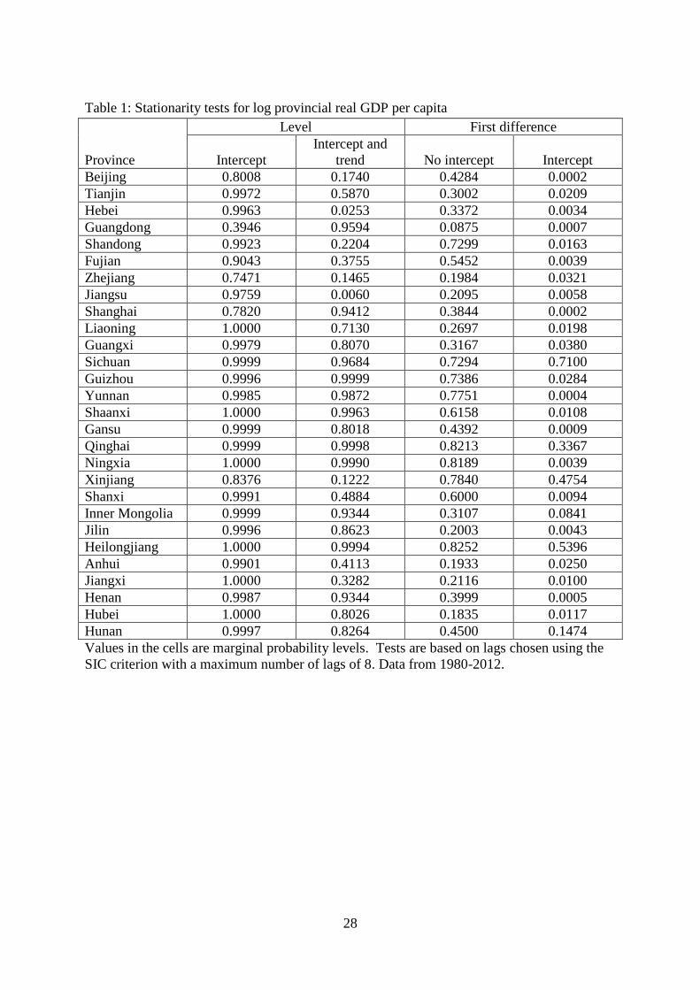
Table 1: Stationarity tests for log provincial real GDP per capita
Province
Level First difference
Intercept Intercept and
trend No intercept Intercept Beijing 0.8008 0.1740 0.4284 0.0002 Tianjin 0.9972 0.5870 0.3002 0.0209 Hebei 0.9963 0.0253 0.3372 0.0034 Guangdong 0.3946 0.9594 0.0875 0.0007 Shandong 0.9923 0.2204 0.7299 0.0163 Fujian 0.9043 0.3755 0.5452 0.0039 Zhejiang 0.7471 0.1465 0.1984 0.0321 Jiangsu 0.9759 0.0060 0.2095 0.0058 Shanghai 0.7820 0.9412 0.3844 0.0002 Liaoning 1.0000 0.7130 0.2697 0.0198 Guangxi 0.9979 0.8070 0.3167 0.0380 Sichuan 0.9999 0.9684 0.7294 0.7100 Guizhou 0.9996 0.9999 0.7386 0.0284 Yunnan 0.9985 0.9872 0.7751 0.0004 Shaanxi 1.0000 0.9963 0.6158 0.0108 Gansu 0.9999 0.8018 0.4392 0.0009 Qinghai 0.9999 0.9998 0.8213 0.3367 Ningxia 1.0000 0.9990 0.8189 0.0039 Xinjiang 0.8376 0.1222 0.7840 0.4754 Shanxi 0.9991 0.4884 0.6000 0.0094 Inner Mongolia 0.9999 0.9344 0.3107 0.0841 Jilin 0.9996 0.8623 0.2003 0.0043 Heilongjiang 1.0000 0.9994 0.8252 0.5396 Anhui 0.9901 0.4113 0.1933 0.0250 Jiangxi 1.0000 0.3282 0.2116 0.0100 Henan 0.9987 0.9344 0.3999 0.0005 Hubei 1.0000 0.8026 0.1835 0.0117 Hunan 0.9997 0.8264 0.4500 0.1474 Values in the cells are marginal probability levels. Tests are based on lags chosen using the SIC criterion with a maximum number of lags of 8. Data from 1980-2012.
28
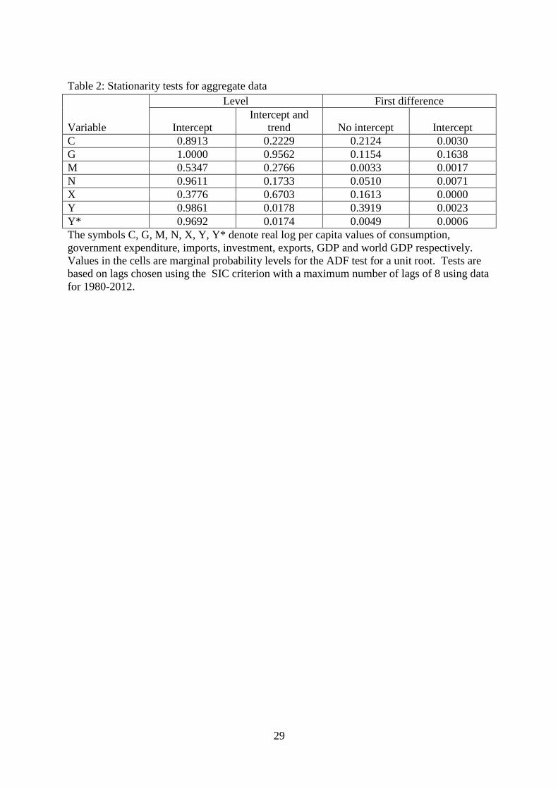
Table 2: Stationarity tests for aggregate data
Variable
Level First difference
Intercept Intercept and
trend No intercept Intercept C 0.8913 0.2229 0.2124 0.0030 G 1.0000 0.9562 0.1154 0.1638 M 0.5347 0.2766 0.0033 0.0017 N 0.9611 0.1733 0.0510 0.0071 X 0.3776 0.6703 0.1613 0.0000 Y 0.9861 0.0178 0.3919 0.0023 Y* 0.9692 0.0174 0.0049 0.0006 The symbols C, G, M, N, X, Y, Y* denote real log per capita values of consumption, government expenditure, imports, investment, exports, GDP and world GDP respectively. Values in the cells are marginal probability levels for the ADF test for a unit root. Tests are based on lags chosen using the SIC criterion with a maximum number of lags of 8 using data for 1980-2012.
29

Table 3: Summary of regional responses to national shocks
Province Rank 2012
One-variable model; Y shock Two-variable model 1953-2012 1953-1979 1980-2012 Y shock N shock
Beijing 3 A* A* B* B B* Tianjin 2 A* A* A A* B Hebei 11 A* A A A C Guangdong 12 B* B* B A* B Shandong 9 C C A C A Fujian 8 A C C A* B Zhejiang 7 B* B* A* A* B Jiangsu 5 B* B* A* A A* Shanghai 1 A A* B* A* B* Liaoning 4 A* A* A* A A* Guangxi 22 B* B* B* A C Sichuan 24 C C A* A A* Guizhou 28 A* A* B B* A Yunnan 27 B B C B A Shaanxi 15 A* A* A* A* A* Gansu 21 B B* A B C Qinghai 19 B B B* B* B* Ningxia 16 B B B* B* B Xinjiang 18 B B B* B* B* Shanxi 17 A* A* B B C Inner Mongolia 6 A* A B* B* A* Jilin 10 A C A B A* Heilongjiang 13 A* A* B* B* B* Anhui 26 C B* A* C A* Jiangxi 23 B* B* A A C Henan 20 A* A A B A Hubei 14 A* A A* A* A Hunan 25 A A B C A Notes: (a) Y and N denote GDP and investment, both at the aggregate level, in real per capita terms. (b) In the body of the table, “A” indicates that the provincial IRF is above the national IRF, “B” that it is below and “C” that it is coincident with. An asterisk indicates that the provincial IRF lies outside the bounds of the national IRF for at least part of the projection period; (c) “Rank 2012” refers to the ranking of the provinces on the basis of their per capita GDP in 2012; (d) the one-variable model refers to a model with only one aggregate variable (Y) and the two-variable model has two aggregate variables (Y and N) both in addition to the 28 provincial GDPs; (e) the two-variable model is estimated over the period 1980-2012.
30

Figure 1: The effects on national GDP of a unit shock to national GDP in a model with one national variable, two lags, sample 1953-2012.
Figure 3: The effects on national GDP of a unit shock to national GDP in a model with one national variable, two lags, sample 1953-1979.
Figure 5: The effects on national GDP of a unit shock to national GDP in a model with one national variable, two lags, sample 1980-2012.
1 2 3 4 5 6 7 8 9 100.6
0.8
1.0
1.2
1.4
1.6
1.8
2.0
1 2 3 4 5 6 7 8 9 100.00
0.25
0.50
0.75
1.00
1.25
1.50
1.75
2.00
2.25
1 2 3 4 5 6 7 8 9 100.0
0.5
1.0
1.5
2.0
2.5
3.0
31

Figure 8: The effects on national GDP of a unit shock to national GDP in a model with two national variables, two lags, sample 1980-2012.
Figure 11: The effects on national GDP of a unit shock to national investment in a model with two national variables, two lags, sample 1980-2012.
1 2 3 4 5 6 7 8 9 10-0.5
0.0
0.5
1.0
1.5
2.0
2.5
3.0
1 2 3 4 5 6 7 8 9 10-1
0
1
2
3
4
5
6
7
32

Figure 7: One-variable model, output shock, 1980-2012
Notes: “A” indicates that the provincial IRF is above the national IRF, “B” that it is below, “C” that it is coincident with and “M” that the provincial data are missing so not included in the simulations. An asterisk indicates that the provincial IRF lies outside the bounds of the national IRF for at least part of the projection period;
MBB*CAA*
33

Figure 10: Two-variable model, output shock, 1980-2012
Notes: “A” indicates that the provincial IRF is above the national IRF, “B” that it is below, “C” that it is coincident with and “M” that the provincial data are missing so not included in the simulations. An asterisk indicates that the provincial IRF lies outside the bounds of the national IRF for at least part of the projection period;
MBB*CAA*
34

Figure 13: Two-variable model, investment shock, 1980-2012
Notes: “A” indicates that the provincial IRF is above the national IRF, “B” that it is below, “C” that it is coincident with and “M” that the provincial data are missing so not included in the simulations. An asterisk indicates that the provincial IRF lies outside the bounds of the national IRF for at least part of the projection period;
MBB*CAA*
35

Figure 2: The effects on provincial GDP of a shock to national GDP in a model with one national variable and two lags; sample 1953-2012.
Provincial cumulative response to unit national GDP shock
dark solid = province, light solid = China, dotted = bounds
Beijing
1 2 3 4 5 6 7 80.6
0.8
1.0
1.2
1.4
1.6
1.8
2.0
Tianjin
1 2 3 4 5 6 7 80.6
0.8
1.0
1.2
1.4
1.6
1.8
2.0
Hebei
1 2 3 4 5 6 7 80.6
0.8
1.0
1.2
1.4
1.6
1.8
2.0
Guangdong
1 2 3 4 5 6 7 80.6
0.8
1.0
1.2
1.4
1.6
1.8
2.0
Shandong
1 2 3 4 5 6 7 80.6
0.8
1.0
1.2
1.4
1.6
1.8
2.0
Fujian
1 2 3 4 5 6 7 80.6
0.8
1.0
1.2
1.4
1.6
1.8
2.0
Zhejiang
1 2 3 4 5 6 7 80.6
0.8
1.0
1.2
1.4
1.6
1.8
2.0
Jiangsu
1 2 3 4 5 6 7 80.50
0.75
1.00
1.25
1.50
1.75
2.00
Shanghai
1 2 3 4 5 6 7 80.6
0.8
1.0
1.2
1.4
1.6
1.8
2.0
Niaoning
1 2 3 4 5 6 7 80.5
1.0
1.5
2.0
2.5
3.0
Guangxi
1 2 3 4 5 6 7 80.6
0.8
1.0
1.2
1.4
1.6
1.8
2.0
Sichuan
1 2 3 4 5 6 7 80.6
0.8
1.0
1.2
1.4
1.6
1.8
2.0
Guizhou
1 2 3 4 5 6 7 80.6
0.8
1.0
1.2
1.4
1.6
1.8
2.0
2.2
Yunnan
1 2 3 4 5 6 7 80.6
0.8
1.0
1.2
1.4
1.6
1.8
2.0
Shaanxi
1 2 3 4 5 6 7 80.6
0.8
1.0
1.2
1.4
1.6
1.8
2.0
2.2
Gansu
1 2 3 4 5 6 7 80.6
0.8
1.0
1.2
1.4
1.6
1.8
2.0
Qinghai
1 2 3 4 5 6 7 80.6
0.8
1.0
1.2
1.4
1.6
1.8
2.0
Ningxia
1 2 3 4 5 6 7 80.6
0.8
1.0
1.2
1.4
1.6
1.8
2.0
Xinjiang
1 2 3 4 5 6 7 80.6
0.8
1.0
1.2
1.4
1.6
1.8
2.0
Shanxi
1 2 3 4 5 6 7 80.6
0.8
1.0
1.2
1.4
1.6
1.8
2.0
2.2
InnerMongolia
1 2 3 4 5 6 7 80.6
0.8
1.0
1.2
1.4
1.6
1.8
2.0
Jilin
1 2 3 4 5 6 7 80.6
0.8
1.0
1.2
1.4
1.6
1.8
2.0
Heilongjiang
1 2 3 4 5 6 7 80.6
0.8
1.0
1.2
1.4
1.6
1.8
2.0
Anhui
1 2 3 4 5 6 7 80.6
0.8
1.0
1.2
1.4
1.6
1.8
2.0
Jiangxi
1 2 3 4 5 6 7 80.6
0.8
1.0
1.2
1.4
1.6
1.8
2.0
Henan
1 2 3 4 5 6 7 80.6
0.8
1.0
1.2
1.4
1.6
1.8
2.0
Hubei
1 2 3 4 5 6 7 80.6
0.8
1.0
1.2
1.4
1.6
1.8
2.0
Hunan
1 2 3 4 5 6 7 80.6
0.8
1.0
1.2
1.4
1.6
1.8
2.0
36

Figure 4: The effects on provincial GDP of a shock to national GDP in a model with one national variable and two lags; sample 1953-1979.
Provincial cumulative response to unit national GDP shock
dark solid = province, light solid = China, dotted = bounds
Beijing
1 2 3 4 5 6 7 80.00
0.25
0.50
0.75
1.00
1.25
1.50
1.75
2.00
2.25
Tianjin
1 2 3 4 5 6 7 80.00
0.25
0.50
0.75
1.00
1.25
1.50
1.75
2.00
2.25
Hebei
1 2 3 4 5 6 7 80.00
0.25
0.50
0.75
1.00
1.25
1.50
1.75
2.00
2.25
Guangdong
1 2 3 4 5 6 7 80.00
0.25
0.50
0.75
1.00
1.25
1.50
1.75
2.00
2.25
Shandong
1 2 3 4 5 6 7 80.00
0.25
0.50
0.75
1.00
1.25
1.50
1.75
2.00
2.25
Fujian
1 2 3 4 5 6 7 80.00
0.25
0.50
0.75
1.00
1.25
1.50
1.75
2.00
2.25
Zhejiang
1 2 3 4 5 6 7 80.00
0.25
0.50
0.75
1.00
1.25
1.50
1.75
2.00
2.25
Jiangsu
1 2 3 4 5 6 7 80.00
0.25
0.50
0.75
1.00
1.25
1.50
1.75
2.00
2.25
Shanghai
1 2 3 4 5 6 7 80.00
0.25
0.50
0.75
1.00
1.25
1.50
1.75
2.00
2.25
Niaoning
1 2 3 4 5 6 7 80.0
0.5
1.0
1.5
2.0
2.5
3.0
Guangxi
1 2 3 4 5 6 7 80.00
0.25
0.50
0.75
1.00
1.25
1.50
1.75
2.00
2.25
Sichuan
1 2 3 4 5 6 7 80.00
0.25
0.50
0.75
1.00
1.25
1.50
1.75
2.00
2.25
Guizhou
1 2 3 4 5 6 7 80.00
0.25
0.50
0.75
1.00
1.25
1.50
1.75
2.00
2.25
Yunnan
1 2 3 4 5 6 7 80.00
0.25
0.50
0.75
1.00
1.25
1.50
1.75
2.00
2.25
Shaanxi
1 2 3 4 5 6 7 80.00
0.25
0.50
0.75
1.00
1.25
1.50
1.75
2.00
2.25
Gansu
1 2 3 4 5 6 7 80.00
0.25
0.50
0.75
1.00
1.25
1.50
1.75
2.00
2.25
Qinghai
1 2 3 4 5 6 7 80.00
0.25
0.50
0.75
1.00
1.25
1.50
1.75
2.00
2.25
Ningxia
1 2 3 4 5 6 7 80.00
0.25
0.50
0.75
1.00
1.25
1.50
1.75
2.00
2.25
Xinjiang
1 2 3 4 5 6 7 80.00
0.25
0.50
0.75
1.00
1.25
1.50
1.75
2.00
2.25
Shanxi
1 2 3 4 5 6 7 80.00
0.25
0.50
0.75
1.00
1.25
1.50
1.75
2.00
2.25
InnerMongolia
1 2 3 4 5 6 7 80.00
0.25
0.50
0.75
1.00
1.25
1.50
1.75
2.00
2.25
Jilin
1 2 3 4 5 6 7 80.00
0.25
0.50
0.75
1.00
1.25
1.50
1.75
2.00
2.25
Heilongjiang
1 2 3 4 5 6 7 80.00
0.25
0.50
0.75
1.00
1.25
1.50
1.75
2.00
2.25
Anhui
1 2 3 4 5 6 7 80.00
0.25
0.50
0.75
1.00
1.25
1.50
1.75
2.00
2.25
Jiangxi
1 2 3 4 5 6 7 80.00
0.25
0.50
0.75
1.00
1.25
1.50
1.75
2.00
2.25
Henan
1 2 3 4 5 6 7 80.00
0.25
0.50
0.75
1.00
1.25
1.50
1.75
2.00
2.25
Hubei
1 2 3 4 5 6 7 80.00
0.25
0.50
0.75
1.00
1.25
1.50
1.75
2.00
2.25
Hunan
1 2 3 4 5 6 7 80.00
0.25
0.50
0.75
1.00
1.25
1.50
1.75
2.00
2.25
37

Figure 6: The effects on provincial GDP of a shock to national GDP in a model with one national variable and two lags; sample 1980-2012.
Provincial cumulative response to unit national GDP shock
dark solid = province, light solid = China, dotted = bounds
Beijing
1 2 3 4 5 6 7 80.0
0.5
1.0
1.5
2.0
2.5
3.0
Tianjin
1 2 3 4 5 6 7 80.0
0.5
1.0
1.5
2.0
2.5
3.0
Hebei
1 2 3 4 5 6 7 80.0
0.5
1.0
1.5
2.0
2.5
3.0
Guangdong
1 2 3 4 5 6 7 80.0
0.5
1.0
1.5
2.0
2.5
3.0
Shandong
1 2 3 4 5 6 7 80.0
0.5
1.0
1.5
2.0
2.5
3.0
Fujian
1 2 3 4 5 6 7 80.0
0.5
1.0
1.5
2.0
2.5
3.0
Zhejiang
1 2 3 4 5 6 7 80.0
0.5
1.0
1.5
2.0
2.5
3.0
Jiangsu
1 2 3 4 5 6 7 80.0
0.5
1.0
1.5
2.0
2.5
3.0
Shanghai
1 2 3 4 5 6 7 80.0
0.5
1.0
1.5
2.0
2.5
3.0
Niaoning
1 2 3 4 5 6 7 80.0
0.5
1.0
1.5
2.0
2.5
3.0
Guangxi
1 2 3 4 5 6 7 80.0
0.5
1.0
1.5
2.0
2.5
3.0
Sichuan
1 2 3 4 5 6 7 80.0
0.5
1.0
1.5
2.0
2.5
3.0
Guizhou
1 2 3 4 5 6 7 80.0
0.5
1.0
1.5
2.0
2.5
3.0
Yunnan
1 2 3 4 5 6 7 80.0
0.5
1.0
1.5
2.0
2.5
3.0
Shaanxi
1 2 3 4 5 6 7 80.0
0.5
1.0
1.5
2.0
2.5
3.0
3.5
Gansu
1 2 3 4 5 6 7 80.0
0.5
1.0
1.5
2.0
2.5
3.0
Qinghai
1 2 3 4 5 6 7 80.0
0.5
1.0
1.5
2.0
2.5
3.0
Ningxia
1 2 3 4 5 6 7 80.0
0.5
1.0
1.5
2.0
2.5
3.0
Xinjiang
1 2 3 4 5 6 7 8-0.5
0.0
0.5
1.0
1.5
2.0
2.5
3.0
Shanxi
1 2 3 4 5 6 7 80.0
0.5
1.0
1.5
2.0
2.5
3.0
InnerMongolia
1 2 3 4 5 6 7 80.0
0.5
1.0
1.5
2.0
2.5
3.0
Jilin
1 2 3 4 5 6 7 80.0
0.5
1.0
1.5
2.0
2.5
3.0
Heilongjiang
1 2 3 4 5 6 7 80.0
0.5
1.0
1.5
2.0
2.5
3.0
Anhui
1 2 3 4 5 6 7 80.0
0.5
1.0
1.5
2.0
2.5
3.0
Jiangxi
1 2 3 4 5 6 7 80.0
0.5
1.0
1.5
2.0
2.5
3.0
Henan
1 2 3 4 5 6 7 80.0
0.5
1.0
1.5
2.0
2.5
3.0
Hubei
1 2 3 4 5 6 7 80.0
0.5
1.0
1.5
2.0
2.5
3.0
Hunan
1 2 3 4 5 6 7 80.0
0.5
1.0
1.5
2.0
2.5
3.0
38

Figure 9: The effects on provincial GDP of a unit shock to national GDP in a model with two national variables, two lags, sample 1980-2012.
Provincial cumulative response to unit output shock
dark solid = province, light solid = China, dotted = bounds
Beijing
1 2 3 4 5 6 7 8- 0. 5
0. 0
0. 5
1. 0
1. 5
2. 0
2. 5
Tianjin
1 2 3 4 5 6 7 8- 0. 5
0. 0
0. 5
1. 0
1. 5
2. 0
2. 5
Hebei
1 2 3 4 5 6 7 8- 0. 5
0. 0
0. 5
1. 0
1. 5
2. 0
2. 5
Guangdong
1 2 3 4 5 6 7 8- 0. 5
0. 0
0. 5
1. 0
1. 5
2. 0
2. 5
3. 0
Shandong
1 2 3 4 5 6 7 8- 0. 5
0. 0
0. 5
1. 0
1. 5
2. 0
2. 5
Fujian
1 2 3 4 5 6 7 8- 0. 5
0. 0
0. 5
1. 0
1. 5
2. 0
2. 5
3. 0
Zhejiang
1 2 3 4 5 6 7 8- 0. 5
0. 0
0. 5
1. 0
1. 5
2. 0
2. 5
3. 0
Jiangsu
1 2 3 4 5 6 7 8- 0. 5
0. 0
0. 5
1. 0
1. 5
2. 0
2. 5
Shanghai
1 2 3 4 5 6 7 8- 0. 5
0. 0
0. 5
1. 0
1. 5
2. 0
2. 5
Niaoning
1 2 3 4 5 6 7 8- 0. 5
0. 0
0. 5
1. 0
1. 5
2. 0
2. 5
Guangxi
1 2 3 4 5 6 7 8- 0. 5
0. 0
0. 5
1. 0
1. 5
2. 0
2. 5
Sichuan
1 2 3 4 5 6 7 8- 0. 5
0. 0
0. 5
1. 0
1. 5
2. 0
2. 5
Guizhou
1 2 3 4 5 6 7 8- 0. 5
0. 0
0. 5
1. 0
1. 5
2. 0
2. 5
Yunnan
1 2 3 4 5 6 7 8- 0. 5
0. 0
0. 5
1. 0
1. 5
2. 0
2. 5
Shaanxi
1 2 3 4 5 6 7 8- 0. 5
0. 0
0. 5
1. 0
1. 5
2. 0
2. 5
3. 0
3. 5
4. 0
Gansu
1 2 3 4 5 6 7 8- 0. 5
0. 0
0. 5
1. 0
1. 5
2. 0
2. 5
Qinghai
1 2 3 4 5 6 7 8- 1. 0
- 0. 5
0. 0
0. 5
1. 0
1. 5
2. 0
2. 5
Ningxia
1 2 3 4 5 6 7 8- 0. 5
0. 0
0. 5
1. 0
1. 5
2. 0
2. 5
Xinjiang
1 2 3 4 5 6 7 8- 0. 5
0. 0
0. 5
1. 0
1. 5
2. 0
2. 5
Shanxi
1 2 3 4 5 6 7 8- 0. 5
0. 0
0. 5
1. 0
1. 5
2. 0
2. 5
InnerMongolia
1 2 3 4 5 6 7 8- 0. 5
0. 0
0. 5
1. 0
1. 5
2. 0
2. 5
Jilin
1 2 3 4 5 6 7 8- 0. 5
0. 0
0. 5
1. 0
1. 5
2. 0
2. 5
Heiongjiang
1 2 3 4 5 6 7 8- 0. 5
0. 0
0. 5
1. 0
1. 5
2. 0
2. 5
Anhui
1 2 3 4 5 6 7 8- 0. 5
0. 0
0. 5
1. 0
1. 5
2. 0
2. 5
Jiangxi
1 2 3 4 5 6 7 8- 0. 5
0. 0
0. 5
1. 0
1. 5
2. 0
2. 5
Henan
1 2 3 4 5 6 7 8- 0. 5
0. 0
0. 5
1. 0
1. 5
2. 0
2. 5
Hubei
1 2 3 4 5 6 7 8- 0. 5
0. 0
0. 5
1. 0
1. 5
2. 0
2. 5
Hunan
1 2 3 4 5 6 7 8- 0. 5
0. 0
0. 5
1. 0
1. 5
2. 0
2. 5
39
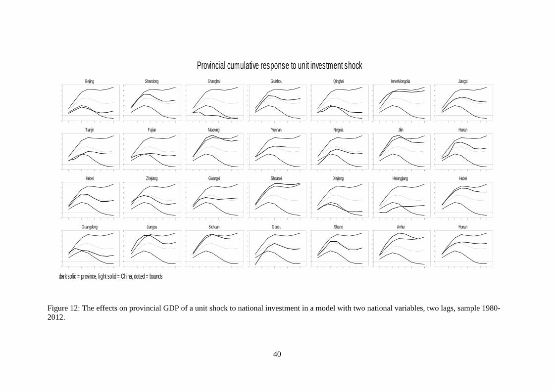
Figure 12: The effects on provincial GDP of a unit shock to national investment in a model with two national variables, two lags, sample 1980-2012.
Provincial cumulative response to unit investment shock
dark solid = province, light solid = China, dotted = bounds
Beijing
1 2 3 4 5 6 7 8- 1
0
1
2
3
4
5
6
Tianjin
1 2 3 4 5 6 7 8- 1
0
1
2
3
4
5
6
Hebei
1 2 3 4 5 6 7 8- 1
0
1
2
3
4
5
6
Guangdong
1 2 3 4 5 6 7 8- 1
0
1
2
3
4
5
6
Shandong
1 2 3 4 5 6 7 8- 1
0
1
2
3
4
5
6
Fujian
1 2 3 4 5 6 7 8- 1
0
1
2
3
4
5
6
Zhejiang
1 2 3 4 5 6 7 8- 1
0
1
2
3
4
5
6
Jiangsu
1 2 3 4 5 6 7 8- 1
0
1
2
3
4
5
6
Shanghai
1 2 3 4 5 6 7 8- 1
0
1
2
3
4
5
6
Niaoning
1 2 3 4 5 6 7 8- 1
0
1
2
3
4
5
6
Guangxi
1 2 3 4 5 6 7 8- 1
0
1
2
3
4
5
6
Sichuan
1 2 3 4 5 6 7 8- 1
0
1
2
3
4
5
6
Guizhou
1 2 3 4 5 6 7 8- 1
0
1
2
3
4
5
6
Yunnan
1 2 3 4 5 6 7 8- 1
0
1
2
3
4
5
6
Shaanxi
1 2 3 4 5 6 7 8- 1
0
1
2
3
4
5
6
Gansu
1 2 3 4 5 6 7 8- 1
0
1
2
3
4
5
6
Qinghai
1 2 3 4 5 6 7 8- 1
0
1
2
3
4
5
6
Ningxia
1 2 3 4 5 6 7 8- 1
0
1
2
3
4
5
6
Xinjiang
1 2 3 4 5 6 7 8- 1
0
1
2
3
4
5
6
Shanxi
1 2 3 4 5 6 7 8- 1
0
1
2
3
4
5
6
InnerMongolia
1 2 3 4 5 6 7 8- 1
0
1
2
3
4
5
6
Jilin
1 2 3 4 5 6 7 8- 1
0
1
2
3
4
5
6
Heiongjiang
1 2 3 4 5 6 7 8- 1
0
1
2
3
4
5
6
Anhui
1 2 3 4 5 6 7 8- 1
0
1
2
3
4
5
6
7
Jiangxi
1 2 3 4 5 6 7 8- 1
0
1
2
3
4
5
6
Henan
1 2 3 4 5 6 7 8- 1
0
1
2
3
4
5
6
Hubei
1 2 3 4 5 6 7 8- 1
0
1
2
3
4
5
6
Hunan
1 2 3 4 5 6 7 8- 1
0
1
2
3
4
5
6
40

Editor, UWA Economics Discussion Papers: Ernst Juerg Weber Business School – Economics University of Western Australia 35 Sterling Hwy Crawley WA 6009 Australia Email: [email protected] The Economics Discussion Papers are available at: 1980 – 2002: http://ecompapers.biz.uwa.edu.au/paper/PDF%20of%20Discussion%20Papers/ Since 2001: http://ideas.repec.org/s/uwa/wpaper1.html Since 2004: http://www.business.uwa.edu.au/school/disciplines/economics
ECONOMICS DISCUSSION PAPERS 2012
DP NUMBER AUTHORS TITLE
12.01 Clements, K.W., Gao, G., and Simpson, T.
DISPARITIES IN INCOMES AND PRICES INTERNATIONALLY
12.02 Tyers, R. THE RISE AND ROBUSTNESS OF ECONOMIC FREEDOM IN CHINA
12.03 Golley, J. and Tyers, R. DEMOGRAPHIC DIVIDENDS, DEPENDENCIES AND ECONOMIC GROWTH IN CHINA AND INDIA
12.04 Tyers, R. LOOKING INWARD FOR GROWTH
12.05 Knight, K. and McLure, M. THE ELUSIVE ARTHUR PIGOU
12.06 McLure, M. ONE HUNDRED YEARS FROM TODAY: A. C. PIGOU’S WEALTH AND WELFARE
12.07 Khuu, A. and Weber, E.J. HOW AUSTRALIAN FARMERS DEAL WITH RISK
12.08 Chen, M. and Clements, K.W. PATTERNS IN WORLD METALS PRICES
12.09 Clements, K.W. UWA ECONOMICS HONOURS
12.10 Golley, J. and Tyers, R. CHINA’S GENDER IMBALANCE AND ITS ECONOMIC PERFORMANCE
12.11 Weber, E.J. AUSTRALIAN FISCAL POLICY IN THE AFTERMATH OF THE GLOBAL FINANCIAL CRISIS
12.12 Hartley, P.R. and Medlock III, K.B. CHANGES IN THE OPERATIONAL EFFICIENCY OF NATIONAL OIL COMPANIES
12.13 Li, L. HOW MUCH ARE RESOURCE PROJECTS WORTH? A CAPITAL MARKET PERSPECTIVE
12.14 Chen, A. and Groenewold, N. THE REGIONAL ECONOMIC EFFECTS OF A REDUCTION IN CARBON EMISSIONS AND AN EVALUATION OF OFFSETTING POLICIES IN CHINA
12.15 Collins, J., Baer, B. and Weber, E.J. SEXUAL SELECTION, CONSPICUOUS CONSUMPTION AND ECONOMIC GROWTH
41

12.16 Wu, Y. TRENDS AND PROSPECTS IN CHINA’S R&D SECTOR
12.17 Cheong, T.S. and Wu, Y. INTRA-PROVINCIAL INEQUALITY IN CHINA: AN ANALYSIS OF COUNTY-LEVEL DATA
12.18 Cheong, T.S. THE PATTERNS OF REGIONAL INEQUALITY IN CHINA
12.19 Wu, Y. ELECTRICITY MARKET INTEGRATION: GLOBAL TRENDS AND IMPLICATIONS FOR THE EAS REGION
12.20 Knight, K. EXEGESIS OF DIGITAL TEXT FROM THE HISTORY OF ECONOMIC THOUGHT: A COMPARATIVE EXPLORATORY TEST
12.21 Chatterjee, I. COSTLY REPORTING, EX-POST MONITORING, AND COMMERCIAL PIRACY: A GAME THEORETIC ANALYSIS
12.22 Pen, S.E. QUALITY-CONSTANT ILLICIT DRUG PRICES
12.23 Cheong, T.S. and Wu, Y. REGIONAL DISPARITY, TRANSITIONAL DYNAMICS AND CONVERGENCE IN CHINA
12.24 Ezzati, P. FINANCIAL MARKETS INTEGRATION OF IRAN WITHIN THE MIDDLE EAST AND WITH THE REST OF THE WORLD
12.25 Kwan, F., Wu, Y. and Zhuo, S. RE-EXAMINATION OF THE SURPLUS AGRICULTURAL LABOUR IN CHINA
12.26 Wu, Y. R&D BEHAVIOUR IN CHINESE FIRMS
12.27 Tang, S.H.K. and Yung, L.C.W. MAIDS OR MENTORS? THE EFFECTS OF LIVE-IN FOREIGN DOMESTIC WORKERS ON SCHOOL CHILDREN’S EDUCATIONAL ACHIEVEMENT IN HONG KONG
12.28 Groenewold, N. AUSTRALIA AND THE GFC: SAVED BY ASTUTE FISCAL POLICY?
42

ECONOMICS DISCUSSION PAPERS 2013
DP NUMBER AUTHORS TITLE
13.01 Chen, M., Clements, K.W. and Gao, G.
THREE FACTS ABOUT WORLD METAL PRICES
13.02 Collins, J. and Richards, O. EVOLUTION, FERTILITY AND THE AGEING POPULATION
13.03 Clements, K., Genberg, H., Harberger, A., Lothian, J., Mundell, R., Sonnenschein, H. and Tolley, G.
LARRY SJAASTAD, 1934-2012
13.04 Robitaille, M.C. and Chatterjee, I. MOTHERS-IN-LAW AND SON PREFERENCE IN INDIA
13.05 Clements, K.W. and Izan, I.H.Y. REPORT ON THE 25TH PHD CONFERENCE IN ECONOMICS AND BUSINESS
13.06 Walker, A. and Tyers, R. QUANTIFYING AUSTRALIA’S “THREE SPEED” BOOM
13.07 Yu, F. and Wu, Y. PATENT EXAMINATION AND DISGUISED PROTECTION
13.08 Yu, F. and Wu, Y. PATENT CITATIONS AND KNOWLEDGE SPILLOVERS: AN ANALYSIS OF CHINESE PATENTS REGISTER IN THE US
13.09 Chatterjee, I. and Saha, B. BARGAINING DELEGATION IN MONOPOLY
13.10 Cheong, T.S. and Wu, Y. GLOBALIZATION AND REGIONAL INEQUALITY IN CHINA
13.11 Cheong, T.S. and Wu, Y. INEQUALITY AND CRIME RATES IN CHINA
13.12 Robertson, P.E. and Ye, L. ON THE EXISTENCE OF A MIDDLE INCOME TRAP
13.13 Robertson, P.E. THE GLOBAL IMPACT OF CHINA’S GROWTH
13.14 Hanaki, N., Jacquemet, N., Luchini, S., and Zylbersztejn, A.
BOUNDED RATIONALITY AND STRATEGIC UNCERTAINTY IN A SIMPLE DOMINANCE SOLVABLE GAME
13.15 Okatch, Z., Siddique, A. and Rammohan, A.
DETERMINANTS OF INCOME INEQUALITY IN BOTSWANA
13.16 Clements, K.W. and Gao, G. A MULTI-MARKET APPROACH TO MEASURING THE CYCLE
13.17 Chatterjee, I. and Ray, R. THE ROLE OF INSTITUTIONS IN THE INCIDENCE OF CRIME AND CORRUPTION
13.18 Fu, D. and Wu, Y. EXPORT SURVIVAL PATTERN AND DETERMINANTS OF CHINESE MANUFACTURING FIRMS
13.19 Shi, X., Wu, Y. and Zhao, D. KNOWLEDGE INTENSIVE BUSINESS SERVICES AND THEIR IMPACT ON INNOVATION IN CHINA
13.20 Tyers, R., Zhang, Y. and Cheong, T.S.
CHINA’S SAVING AND GLOBAL ECONOMIC PERFORMANCE
13.21 Collins, J., Baer, B. and Weber, E.J. POPULATION, TECHNOLOGICAL PROGRESS AND THE EVOLUTION OF INNOVATIVE POTENTIAL
13.22 Hartley, P.R. THE FUTURE OF LONG-TERM LNG CONTRACTS
13.23 Tyers, R. A SIMPLE MODEL TO STUDY GLOBAL MACROECONOMIC INTERDEPENDENCE
43

13.24 McLure, M. REFLECTIONS ON THE QUANTITY THEORY: PIGOU IN 1917 AND PARETO IN 1920-21
13.25 Chen, A. and Groenewold, N. REGIONAL EFFECTS OF AN EMISSIONS-REDUCTION POLICY IN CHINA: THE IMPORTANCE OF THE GOVERNMENT FINANCING METHOD
13.26 Siddique, M.A.B. TRADE RELATIONS BETWEEN AUSTRALIA AND THAILAND: 1990 TO 2011
13.27 Li, B. and Zhang, J. GOVERNMENT DEBT IN AN INTERGENERATIONAL MODEL OF ECONOMIC GROWTH, ENDOGENOUS FERTILITY, AND ELASTIC LABOR WITH AN APPLICATION TO JAPAN
13.28 Robitaille, M. and Chatterjee, I. SEX-SELECTIVE ABORTIONS AND INFANT MORTALITY IN INDIA: THE ROLE OF PARENTS’ STATED SON PREFERENCE
13.29 Ezzati, P. ANALYSIS OF VOLATILITY SPILLOVER EFFECTS: TWO-STAGE PROCEDURE BASED ON A MODIFIED GARCH-M
13.30 Robertson, P. E. DOES A FREE MARKET ECONOMY MAKE AUSTRALIA MORE OR LESS SECURE IN A GLOBALISED WORLD?
13.31 Das, S., Ghate, C. and Robertson, P. E.
REMOTENESS AND UNBALANCED GROWTH: UNDERSTANDING DIVERGENCE ACROSS INDIAN DISTRICTS
13.32 Robertson, P.E. and Sin, A. MEASURING HARD POWER: CHINA’S ECONOMIC GROWTH AND MILITARY CAPACITY
13.33 Wu, Y. TRENDS AND PROSPECTS FOR THE RENEWABLE ENERGY SECTOR IN THE EAS REGION
13.34 Yang, S., Zhao, D., Wu, Y. and Fan, J.
REGIONAL VARIATION IN CARBON EMISSION AND ITS DRIVING FORCES IN CHINA: AN INDEX DECOMPOSITION ANALYSIS
44

ECONOMICS DISCUSSION PAPERS 2014
DP NUMBER AUTHORS TITLE
14.01 Boediono, Vice President of the Republic of Indonesia
THE CHALLENGES OF POLICY MAKING IN A YOUNG DEMOCRACY: THE CASE OF INDONESIA (52ND SHANN MEMORIAL LECTURE, 2013)
14.02 Metaxas, P.E. and Weber, E.J. AN AUSTRALIAN CONTRIBUTION TO INTERNATIONAL TRADE THEORY: THE DEPENDENT ECONOMY MODEL
14.03 Fan, J., Zhao, D., Wu, Y. and Wei, J. CARBON PRICING AND ELECTRICITY MARKET REFORMS IN CHINA
14.04 McLure, M. A.C. PIGOU’S MEMBERSHIP OF THE ‘CHAMBERLAIN-BRADBURY’ COMMITTEE. PART I: THE HISTORICAL CONTEXT
14.05 McLure, M. A.C. PIGOU’S MEMBERSHIP OF THE ‘CHAMBERLAIN-BRADBURY’ COMMITTEE. PART II: ‘TRANSITIONAL’ AND ‘ONGOING’ ISSUES
14.06 King, J.E. and McLure, M. HISTORY OF THE CONCEPT OF VALUE
14.07 Williams, A. A GLOBAL INDEX OF INFORMATION AND POLITICAL TRANSPARENCY
14.08 Knight, K. A.C. PIGOU’S THE THEORY OF UNEMPLOYMENT AND ITS CORRIGENDA: THE LETTERS OF MAURICE ALLEN, ARTHUR L. BOWLEY, RICHARD KAHN AND DENNIS ROBERTSON
14.09
Cheong, T.S. and Wu, Y. THE IMPACTS OF STRUCTURAL RANSFORMATION AND INDUSTRIAL UPGRADING ON REGIONAL INEQUALITY IN CHINA
14.10 Chowdhury, M.H., Dewan, M.N.A., Quaddus, M., Naude, M. and Siddique, A.
GENDER EQUALITY AND SUSTAINABLE DEVELOPMENT WITH A FOCUS ON THE COASTAL FISHING COMMUNITY OF BANGLADESH
14.11 Bon, J. UWA DISCUSSION PAPERS IN ECONOMICS: THE FIRST 750
14.12 Finlay, K. and Magnusson, L.M. BOOTSTRAP METHODS FOR INFERENCE WITH CLUSTER-SAMPLE IV MODELS
14.13 Chen, A. and Groenewold, N. THE EFFECTS OF MACROECONOMIC SHOCKS ON THE DISTRIBUTION OF PROVINCIAL OUTPUT IN CHINA: ESTIMATES FROM A RESTRICTED VAR MODEL
14.14 Hartley, P.R. and Medlock III, K.B. THE VALLEY OF DEATH FOR NEW ENERGY TECHNOLOGIES
14.15 Hartley, P.R., Medlock III, K.B., Temzelides, T. and Zhang, X.
LOCAL EMPLOYMENT IMPACT FROM COMPETING ENERGY SOURCES: SHALE GAS VERSUS WIND GENERATION IN TEXAS
14.16 Tyers, R. and Zhang, Y. SHORT RUN EFFECTS OF THE ECONOMIC REFORM AGENDA
14.17 Clements, K.W., Si, J. and Simpson, T. UNDERSTANDING NEW RESOURCE PROJECTS
45