Embed Size (px)
Citation preview

Economical Hydrothermal Coordination using
Intelligent Computational Techniques
By
Fayyaz Ahmad
CIIT/FA13-PEE-001/WAH
PhD Thesis
In
Electrical Engineering
COMSATS University Islamabad
Wah Campus - Pakistan
Fall, 2019

ii
COMSATS University Islamabad
Economical Hydrothermal Coordination using
Intelligent Computational Techniques
A Thesis Presented to
COMSATS University Islamabad
In partial fulfillment
of the requirement for the degree of
PhD (Electrical Engineering)
By
Fayyaz Ahmad
CIIT/FA13-PEE-001/WAH
Fall, 2019

iii
Economical Hydrothermal Coordination using Intelligent Computational Techniques
A Post Graduate Thesis submitted to the Department of Electrical and
Computer Engineering as partial fulfillment of the requirement for the award of
PhD (Electrical Engineering).
Supervisor
Dr. Muhammad Iqbal Associate Professor, Department of Electrical and Computer Engineering, COMSATS University Islamabad (CUI), Wah Campus
Name Registration Number
Fayyaz Ahmad CIIT/FA13-PEE-001/WAH


viii
DEDICATION
To Almighty ALLAH and Holy Prophet Muhammad
(P.B.U.H)
&
To my parents, beloved wife, my dear daughter and my
brave son whose sacrifices have encouraged me to
complete my research work for the accomplishment of
Ph.D.

ix
ACKNOWLEDGEMENTS
I want to start my acknowledgment with the Higher Education Commission (HEC) for
the award of Indigenous Ph.D. Scholarship. I feel that without technical support
provided by my supervisor Dr. Muhammad Iqbal and supervisory committee
especially Dr. Muhammad Naeem and Dr. Muhammad Ashfaq, I would never have
been able to complete my Ph.D. studies research.
I am also grateful to my friends Dr. Usman Ali (The University of Lahore), Engr.
Fahimullah Khanzada (Ministry of Science and Technology), Engr. Mehroz Iqbal
(The University of Engineering and Technology, Taxila), Dr. Danish Mehmood
(Shaheed Zulfikar Ali Bhutto Institute of Science and Technology), Dr. Nadir Ali
Shah (COMSATS University Islamabad), Zeeshan Anjum (The University of
Engineering and Technology, Taxila), Dr. Kamran Nazir (National University of
Technology), Engr. Rashid Jamil Satti (Swedish College), Engr. Muhammad Saeed
(National Transmission and Dispatch Company), Engr. Ali Tariq (Water and Power
Development Authority) and Dr. Muhammad Zubair (Information Technology
University) for their generous support and insightful guidance.
Fayyaz Ahmad
CIIT/FA13-PEE-001/WAH
x
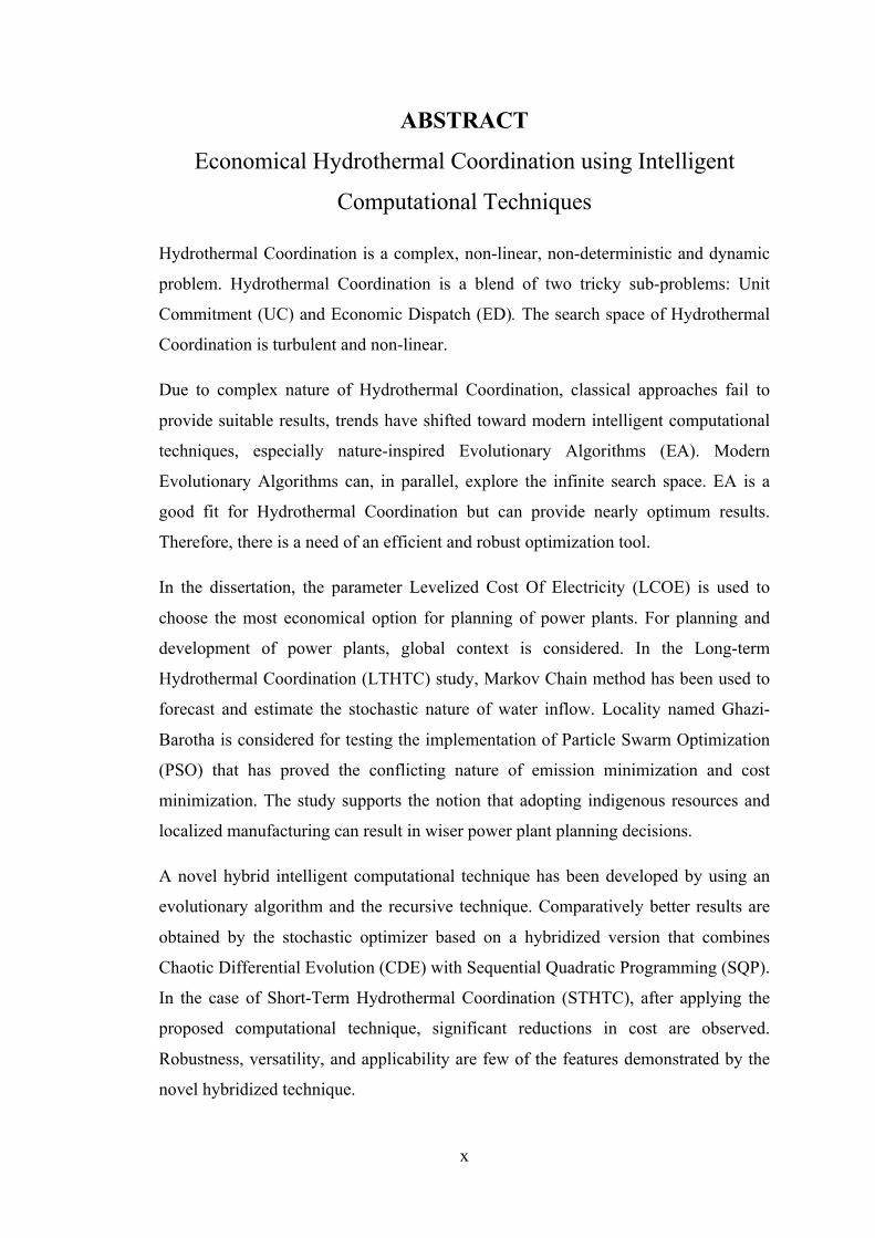
ABSTRACT
Economical Hydrothermal Coordination using Intelligent
Computational Techniques
Hydrothermal Coordination is a complex, non-linear, non-deterministic and dynamic
problem. Hydrothermal Coordination is a blend of two tricky sub-problems: Unit
Commitment (UC) and Economic Dispatch (ED). The search space of Hydrothermal
Coordination is turbulent and non-linear.
Due to complex nature of Hydrothermal Coordination, classical approaches fail to
provide suitable results, trends have shifted toward modern intelligent computational
techniques, especially nature-inspired Evolutionary Algorithms (EA). Modern
Evolutionary Algorithms can, in parallel, explore the infinite search space. EA is a
good fit for Hydrothermal Coordination but can provide nearly optimum results.
Therefore, there is a need of an efficient and robust optimization tool.
In the dissertation, the parameter Levelized Cost Of Electricity (LCOE) is used to
choose the most economical option for planning of power plants. For planning and
development of power plants, global context is considered. In the Long-term
Hydrothermal Coordination (LTHTC) study, Markov Chain method has been used to
forecast and estimate the stochastic nature of water inflow. Locality named Ghazi-
Barotha is considered for testing the implementation of Particle Swarm Optimization
(PSO) that has proved the conflicting nature of emission minimization and cost
minimization. The study supports the notion that adopting indigenous resources and
localized manufacturing can result in wiser power plant planning decisions.
A novel hybrid intelligent computational technique has been developed by using an
evolutionary algorithm and the recursive technique. Comparatively better results are
obtained by the stochastic optimizer based on a hybridized version that combines
Chaotic Differential Evolution (CDE) with Sequential Quadratic Programming (SQP).
In the case of Short-Term Hydrothermal Coordination (STHTC), after applying the
proposed computational technique, significant reductions in cost are observed.
Robustness, versatility, and applicability are few of the features demonstrated by the
novel hybridized technique.
xi
Table of Contents
1 Introduction .................................................................................................... 1
1.1 Chapter Summary ......................................................................... 2
1.2 Introduction ................................................................................... 2
1.3 Problem Statement ........................................................................ 3
1.4 Research Objectives ...................................................................... 4
1.5 Usefulness of the Research ........................................................... 4
1.6 List of Contributions ..................................................................... 5
1.6.1 Published Manuscripts ...................................................... 5
1.6.2 Submitted Manuscripts ...................................................... 5
1.7 Thesis Outline ............................................................................... 6
1.8 Chapter Conclusion ....................................................................... 7
2 Literature Review ........................................................................................... 8
2.1 Chapter Summary ......................................................................... 9
2.2 Background ................................................................................... 9
2.3 Literature Survey ......................................................................... 10
2.3.1 Objectives of Hydrothermal Coordination ...................... 22
2.3.2 Constraints of Hydrothermal Coordination ..................... 23
2.3.3 Optimization Techniques Applied to Hydrothermal
Coordination ................................................................................ 24
2.4 Discussion ................................................................................... 25
2.5 Chapter Conclusion ..................................................................... 27
3 Power Plants Development Trend .............................................................. 28
xii
3.1 Chapter Summary ....................................................................... 29
3.2 Background ................................................................................. 29
3.3 Levelized Cost of Electricity (LCOE) ........................................ 31
3.3.1 Non-Renewable Energy Sources ..................................... 33
3.3.2 Renewable Energy Sources ............................................. 36
3.3.3 Nuclear Power Plants ...................................................... 39
3.4 Trend of Global Electricity Generation and the Resulting GHG
Emissions ............................................................................................... 40
3.4.1 Global Generation ........................................................... 40
3.4.2 Global Emission .............................................................. 43
3.5 Discussion ................................................................................... 44
3.5.1 Cost .................................................................................. 44
3.5.2 Emission .......................................................................... 44
3.5.3 Reliability ........................................................................ 45
3.5.4 Global Emission Control Strategy ................................... 45
3.6 Chapter Conclusion ..................................................................... 46
4 Long-Term Hydrothermal Coordination (LTHTC) ................................. 47
4.1 Chapter Summary ....................................................................... 48
4.2 Background ................................................................................. 48
4.3 Electricity Sector in Pakistan ...................................................... 49
4.4 System Model and Problem Formulation ................................... 49
4.4.1 Hydropower Power Plant and Load Demand .................. 49
4.4.2 Thermal System Modeling .............................................. 58
4.5 Proposed Algorithm and Settings ............................................... 62
4.5.1 Proposed Algorithm ........................................................ 62

xiii
4.5.2 Particle Swarm Optimization (PSO) Attributes .............. 64
4.6 Simulation Results ...................................................................... 64
4.7 Chapter Conclusion ..................................................................... 73
5 Short-Term Hydrothermal Coordination (STHTC) ................................. 74
5.1 Chapter Summary ....................................................................... 75
5.2 Related Work and Case-studies .................................................. 75
5.3 Problem Formulation .................................................................. 79
5.3.1 System Constraints .......................................................... 79
5.4 Chaotic Differential Evolution (CDE) and Quadratic
Programming (QP) ................................................................................. 80
5.5 Simulation and Results ................................................................ 87
5.5.1 Case Study I: ................................................................... 88
5.5.2 Case Study II ................................................................... 90
5.5.3 Case Study III .................................................................. 91
5.5.4 Case Study IV .................................................................. 92
5.6 Comparative Analysis of the Results .......................................... 94
5.6.1 Improvements Observed in Applicability, Robustness and
Versatility .................................................................................. 100
5.6.2 Efficiency of the Proposed Algorithm ........................... 101
5.7 Multi-objective Case Study ....................................................... 101
5.8 Chapter Conclusion ................................................................... 104
6 Conclusion ................................................................................................... 105
6.1 Conclusion ................................................................................ 106
6.2 Future Work .............................................................................. 108
7 References ................................................................................................... 109

xiv
List of Figures
Figure 2.1: Global Electricity Generation by Source (2017) ....................................... 10
Figure 2.2: Flow chart of Genetic Algorithm (GA) ..................................................... 16
Figure 2.3: Objectives of Hydrothermal Coordination ................................................ 22
Figure 2.4: Constraints of Hydrothermal Coordination ............................................... 24
Figure 2.5: Optimization Techniques Applied to Hydrothermal Coordination ........... 25
Figure 3.1: Types of power generation systems with respect to the energy source ..... 30
Figure 3.2: Factors Affecting the Levelized Cost of Electricity (LCOE) .................... 32
Figure 3.3: Global Levelized Cost of Electricity (LCOE) of Power Generation in 2017
...................................................................................................................................... 33
Figure 3.4: Trend of coal-based electricity generation (2008-2017) ........................... 34
Figure 3.5: Trend of global electricity generation by oil (2008-2017) ....................... 35
Figure 3.6: Trend of global electricity generation by gas (2008-2017) ....................... 36
Figure 3.7: Trend of hydel generation in the world in the last decade ........................ 37
Figure 3.8: Trend of geothermal energy generation in the world for the last decade .. 38
Figure 3.9: Trend of biomass energy generation in the world for the last decade ....... 38
Figure 3.10: International trend of nuclear energy generation in the last decade ........ 39
Figure 3.11: Global electricity generation trend observed in the last decade .............. 41
Figure 3.12: G-20 countries power generation major resource [108, 109] .................. 42
Figure 3.13: Percentage emission in the world by different power sources in 2017 ... 44
xv
Figure 3.14: Emission Control Strategy ....................................................................... 46
Figure 4.1: State diagrams of the period January to December ................................... 54
Figure 4.2: Particle Swarm Optimization (PSO) flow chart ........................................ 63
Figure 4.3: Convergence Behavior of Combined Fuel and Emission Minimization
(CFEM) ........................................................................................................................ 65
Figure 4.4: Expected Water Inflow and Discharge ...................................................... 70
Figure 4.5: Reservoir storage profile throughout the year ........................................... 70
Figure 4.6: Load demand vs generation by power plants ............................................ 71
Figure 4.7: Cost of Fuel with respect to Objectives ..................................................... 71
Figure 4.8: Emission with respect to objectives .......................................................... 72
Figure 4.9: Pareto Function of fuel cost and the resulting emissions .......................... 73
Figure 5.1: Flow Chart of Sequential Quadretic Programming ................................... 76
Figure 5.2: Flow Chart of Differential Evolution ........................................................ 78
Figure 5.3: Flow Chart of Chaotic Differential Evolution ........................................... 82
Figure 5.4: Flow Chart of Chaotic Differential Evolution (CDE) Hybridized with SQP
...................................................................................................................................... 85
Figure 5.5: (a) Behavior of the fitness function evaluation; (b) Absolute error of
thermal generation for 100 intervals ............................................................................ 89
Figure 5.6: Behavior of the fitness function value (a) and absolute error of thermal
generation for 100 intervals in (b) ............................................................................... 90
Figure 5.7: (a) Behavior of the fitness function evaluation; (b) Absolute error of
thermal generation for 100 intervals ............................................................................ 91
Figure 5.8: (a) Behavior of the fitness function evaluation; (b) Absolute error of
thermal generation for 100 intervals ............................................................................ 94

xvi
Figure 5.9: Comparative analysis of the computational budget for case studies I, II,
III and IV ...................................................................................................................... 96
Figure 5.10: Convergence behavior of the fitness for case studies I to IV using hybrid
approach ....................................................................................................................... 99
Figure 5.11: Pareto Front for Multi-objective Case Study ........................................ 103
xvii
List of Tables
Table 3.1: Global CO2 emissions trend ........................................................................ 40
Table 4.1: Average monthly inflow of Ghazi Barotha site from 2010 to 2017 in
Cumecs ......................................................................................................................... 50
Table 4.2: Monthly Average Load-demand ................................................................. 51
Table 4.3: Discretization of States ............................................................................... 53
Table 4.4: State Table from January to June ................................................................ 55
Table 4.5: State Table from July to December ............................................................ 56
Table 4.6: Fuel cost-coefficients and the limitations ................................................... 59
Table 4.7: Emission cost-coefficients and limits ......................................................... 59
Table 4.8: Results of scheduling power plants against the objectives 1,2,3 ................ 66
Table 4.9: Results of scheduling power plants against the objectives 4,5,6 ................ 67
Table 4.10: Results of scheduling power plants against the objectives 7,8,9 .............. 68
Table 4.11: Results of scheduling power plants against the objectives 10, 11 ............ 69
Table 5.1: Parameter Values/Settings for Chaotic Differential Evolution and
Sequential Quadratic Programming ............................................................................. 87
Table 5.2: Optimal Hydrothermal Generation (MW) for Case Study I ....................... 88
Table 5.3: Optimal Hydrothermal Generation (MW) for Case Study II ...................... 89
Table 5.4: Results of generation hydro and thermal generations ................................. 90
Table 5.5: Optimal Hydrothermal Generation (MW) for Case Study III ................... 92
Table 5.6: Optimal Hydrothermal Generation (MW) for Case Study IV ................... 93

xviii
Table 5.7: Comparative study in DE, SQP, and DE-SQP in terms of fitness achieved
...................................................................................................................................... 95
Table 5.8: Comparison between DE, SQP and DE-SQP in term of Load Error .......... 97
Table 5.9: Comparison between DE, SQP, and DE-SQP in term of computational
complexity .................................................................................................................... 98
Table 5.10: Comparison between DE, SQP and DE-SQP in term of cost (US $) ....... 99
Table 5.11: Attributes Observed in our I-IV case studies .......................................... 100
Table 5.12: Efficiency of the Proposed Algorithm .................................................... 101
Table 5.13: Power and heat values in case of extreme objectives ............................. 102
Table 5.14: Percentage of decrease of Cost and Emission ........................................ 103
xix
LIST OF SYMBOLS
Losses due to power transmission at time ‘t’
Total number of thermal units
Cost coefficient for thermal power generation ‘i'
Cost coefficient for thermal power generation ‘i'
Cost coefficient for thermal power generation ‘i'
Cost coefficient for thermal power generation ‘i'
Cost coefficient for thermal power generation ‘i'
Generated output power in time t of thermal unit ‘i'
Maximum thermal generation limits for unit ‘i'
Minimum thermal generation limits for unit ‘i'
Power demand at time ‘t’
Total number of hydroelectric units
Down ramp rate limit of thermal unit ‘i'
Up ramp rate limit of thermal unit ‘i'
The water discharge rate of the jth reservoir at the time ‘t’
The water storage volume of the jth reservoir at the time ‘t’
ltP
THN
THix
THiy
THiz
THiu
THie
THitP
maxTHiP
minTHiP
dtP
hN
iDR
iUR
hjtQ
hjtV

xx
Water storage minimum limit of reservoir ‘j’
Water storage maximum limit of reservoir ‘j’
Generated power from the jth hydroelectric unit at time ‘t’
Power generation coefficient of jth hydroelectric unit
Power generation coefficient of jth hydroelectric unit
Power generation coefficient of jth hydroelectric unit
Power generation coefficient of jth hydroelectric unit
Power generation coefficient of jth hydroelectric unit
Power generation coefficient of jth hydroelectric unit
The lower limit of the jth hydroelectric unit
The upper limit of the jth hydroelectric unit
The minimum water discharge rate of jth reservoir
The maximum water discharge rate of jth reservoir
Time index
Scheduling period
The randomly generated population of candidate solutions
Population size
Short-term Hydrothermal Coordination (STHTC) problem size
minhjV
maxhjV
hjtP
jC1
jC2
jC3
jC4
jC5
jC6
minhjP
maxhjP
minhjQ
maxhjQ
t
T
Pop
Psize
PSTHTCsize
xxi
Weight factor
Crossover rate
Chaotic variable
Cost of the fitness evaluation function
The capital cost of the power plant
The life cycle of the power plant
Operating cost in the year ‘t’
Time value of money
Corporate tax rate
Salvage value of the assets at the end of the life cycle
Energy production
System degradation in the year ‘t’
Depreciation schedule in the year ‘t’
Mass
Work
Volume
Gravitational acceleration
Discharge
℟ Fictional monetary unit
β
Crate
z
fval
cC
cL
cO
Y
Q
vS
Γ
SDt
ds
m
ΔU
V
g
Q
xxii
Storage minimum limits of reservoir ‘j’
Storage maximum limit of reservoir ‘j’
Emission cost coefficient for thermal power generator ‘i'
Emission cost coefficient for thermal power generation ‘i'
Emission cost coefficient for thermal power generation ‘i'
Emission cost coefficient for thermal power generation ‘i'
Emission cost coefficient for thermal power generation ‘i'
Number of rotors
Power output of a generator at time ‘t’
Penalty factor
Efficiency of hydropower plant
Storage at time ‘t’
Expected inflow
Scale parameter
Discharge at time ‘t’
Spillage at time ‘t’
Non-effective discharge
Basic head of reservoir ‘j’
S jmin
S jmax
xTHei
yTHei
zTHei
uTHei
eTHei
Nr
Pt
Ã
ηh
tS
Et
a
Qt
tS
µ t
hj

xxiii
Head correction factor
Exp Expectation
Sti Discrete value state
j Generator number
Nh Total number of hydro generators
fc

xxiv
LIST OF ABBREVIATIONS
LACE Levelized Avoided Cost of Electricity
DE Differential Evolution
SQP Sequential Quadratic Programming
LCOE Levelized Cost of Electricity
ED Economic Dispatch
K.E Kinetic Energy
P.E Potential energy
HTC Hydrothermal Coordination
LTHTC Long-term Hydrothermal Coordination
PSO Particle Swarm Optimization
CDE Chaotic differential evolution
STHTC short-term hydrothermal coordination
ICT Intelligent Computational Techniques
MILP Mixed-Integer Linear Programming
SCUC Short-term Security-Constrained Unit Commitment
PHES Pumped Hydro Energy Storage
UC Unit Commitment
MOABC Multi-Objective Artificial Bee Colony
DEA Data Environmental Analysis
ARIMA Autoregressive Integrated Moving Average
xxv
QOTLBO Quasi-Oppositional Teaching Learning-Based Optimization
ISAPSO Improved Self-adaptive Particle Swarm Optimization
HUCL Hydro Unit Commitment and Loading
HTS Hydrothermal Scheduling
BDI-BFPSO Bacterial Foraging Oriented by Particle Swarm Optimization
AIS Artificial Immune System
OPF Optimal Power Flow
GS Gradient Search
DP Dynamic Programming
EP Evolutionary Programming
DE-SQP Differential Evolution - Sequential Quadratic Programming
RGM Reduced Gradient Method
NRM Newton Raphson Method
GSM Gauss Seidel Method
NMM Nelder-Mead Method
LR Lagrange Relaxation
BD Benders Decomposition
HBA Honey Bee Algorithm
MGA Minority Game Algorithm
BFA Bacterial forging algorithm
FFA Fruit Fly Algorithm

xxvi
QP Quadratic Programming
SAEEP Simulated Annealing Embedded Evolutionary Programming
LEEMA Low-Emissions Electricity Market Analysis
SGA Simple Genetic Algorithm
NPCC National Power Control Center
MINLP Mixed Integer Non-linear Programming
MILP Mixed Integer Linear Programming
GA Genetic Algorithm

1
Introduction
2
1.1 Chapter Summary
This chapter presents an introduction of Hydrothermal Coordination. After that,
problem statement is discussed and later on research objectives are selected. Then the
potential avenues of usefulness of research are discussed. Author contribution in the
knowledge base has been given in the form of submitted and published articles. At the
end of the chapter, layout of the thesis is presented.
1.2 Introduction
The systematic approach of Hydrothermal Coordination results in an optimum mean
of utilizing the available hydro and thermal generation systems keeping in view the
constraints and limitations. Optimum utilization of energy resources by forecasting,
planning, and scheduling of available generation systems have always been a
prominent area in electrical power engineering. Oil prices have been showing an
increasing trend since the 1970s. As an immediate impact, in 1973, revenue worth
about twenty percent of the United States (US) federal budget went into various fuels
for generating electrical energy. The fuel cost continued on escalating and this in turn
effected the case of electricity. In the early 1980s, according to estimates, the US
spent about over forty percent of its total revenue on the production of electricity. It
motivated electrical power researchers and engineers to develop hydrothermal
coordination.
It is a known reality that thermal fuels are irreplaceable. As a result, academic
endeavors aimed at fuel conservation and reduction of energy costs have experienced
phenomenal growth. Hydrothermal Coordination is a technique used to save fuel costs
and conserve time. Another factor worth consideration is assigning weight to each of
the following two factors, i.e. irrigation and power production. It varies from place to
place. For instance, being an agricultural country, in Pakistan, mostly, the irrigation
facet receives more weight than the electricity element.
Hydroelectric systems are connected in the form of chains, or cascaded manner, and
for interruption-free operation, synchronized coordination is essential among the two
interconnected systems. Such factor must be considered in engineering design.
3
Hydroelectric systems are designed keeping in view the inherent geo-climatic and
weather variables such as water inflow, regional boundaries and storage capacity etc.
This makes them distinctly different and incomparable to each other. Owing to the
aforementioned major factors, operating a hydropower plant is a complicated task and
demands a vigilant multi-pronged approach.
Scheduling hydropower plants is also of surmount importance and can be of two types
i.e. long range and short range. In long-range scheduling, the time period stretches
from few weeks to few years and depends on climate profile and other geo-
topographic features. That is, the capacity of Khanpur Dam will be effected in case of
snowfall and rain on Murree hills, Pakistan. Further, decisions about choosing the
types of power plants are also carried in such scheduling category. Composite
simulation techniques are often used to resolve long-range scheduling problems.
Short-term hydropower scheduling deal with time period ranging from few hours to
few weeks. The best possible option is selected based on trade-off between cost and
endpoint requirements.
Hydrothermal coordination aims to ensure maximum utilization of hydropower plants
with minimum dependency on thermal fuels. It creates a balance among the following
variables: power demand, hydro generators and thermal generators. It also depends on
a number of constraints like water release limit, fuel cost, throttle cost and valve-point
loading.
1.3 Problem Statement
Electricity cycle lies in between production and consumption. Within this cycle, there
are numerous complex processes. One of the serious concerns, here, is the power
generation that is eco-friendly, reliable and economically sustainable. Electricity can
be produced from various sources; however, two of the major contributors are
hydroelectric and thermal power plants as their cumulative share is about 70% of the
world’s generated power.
A choice to select the viable energy generation option depends on its resourcefulness
and trade-offs. Through proper coordination between hydropower plants and thermal
4
power plants, cost minimization, as well as emission reduction, can be achieved.
Classical gradient-based techniques, such as Gauss Seidel and Newton Raphson,
cannot handle Hydrothermal Coordination since it is non-differentiable. Recursive
techniques, e.g. Dynamic Programming, can produce marginal results but require a lot
of computational budgets. One of the latest trends of the last decade is toward the
evolutionary algorithms that can handle the vague data and can produce good results
but they are not able to give optimum results.
HTC is a unique problem so it requires a powerful, robust and efficient optimization
technique that can handle a large search space of many constraints and can produce
optimum results. For such coordination activity to sail smoothly, a trade-off is to be
maintained between power demand and emission.
1.4 Research Objectives
Major objectives of the research work are as follows:
• Use of Mathematical modeling of power plants for economic analysis
• Identification of the constraints and objectives of Hydrothermal Coordination
• Conduct economic analysis of power plants
• Utilization of forecasting technique for stochastic problem
• Cost-minimization of electricity production using intelligent computational
techniques
• Implementation of the Evolutionary Algorithm in local settings
• Hybridization of optimization algorithms to obtain desired results
• Perform a critical comparative analysis of the proposed system and the
existing systems
As an ultimate aim the work will culminate in an intelligent computational technique
that integrates hydroelectric power plants with thermal power plants
1.5 Usefulness of the Research
Energy has a significant share in a country’s developmental budget. Apart from
financial elements, the issue of GHG emission also needs proper consideration. The

5
work aims to resolve the issues of energy-related costs and the associated emissions.
After highlighting the pros and cons of various power generation techniques, the work
results in a valuable power-plants selection mechanism that finds value in the
planning and development of the power sector. Besides, the Markov chain forecasting
method has been used for resource assessment of hydropower energy. The proposed
solution, hybrid algorithm, amalgamates evolutionary algorithm and recursive
technique and shows much better performance than each of its amalgams.
1.6 List of Contributions
1.6.1 Published Manuscripts
Paper 1. Fayyaz et al. (2018) “A novel chaotic differential evolution hybridized with
quadratic programming for short-term hydrothermal coordination.” Neural Computing
and Applications, 30(11), 3533-3544. (IF=4.67)
Paper 2. Fayyaz et al. (2018) “Optimal Allocation of Flexible AC Transmission
System Controllers in Electric Power Networks.” INAE Letters, 3(1), 41-64.
Paper 3. Fayyaz et al., (2015) “A Hybrid Algorithm for Energy Management in
Smart Grid.” Network-Based Information Systems (NBiS), 18th International
Conference on 2015 Sep 2 (pp. 58-63). IEEE.
Paper 4. Fayyaz et al. (2015) “An Energy-Efficient Residential Load Management
System for Multi-Class Appliances in Smart Homes.” Network-Based Information
Systems (NBiS), 18th International Conference on 2015 Sep 2 (pp. 53-57). IEEE.
1.6.2 Submitted Manuscripts
1. Hydrothermal Coordination using Intelligent Computational Techniques (A
Comprehensive Review)
2. Multi-objective Hydrothermal Coordination using Particle Swarm
Optimization (A Case Study)
3. Global Power Generation Development in the Context of Levelized Cost of
Electricity and Emission

6
1.7 Thesis Outline
The write-up comprises of six chapters. First two chapters are dedicated to
introduction and literature review. The third chapter provides a discussion about
developing the power plants trends and strategy. Fourth and fifth chapter present
commentary about Long-term Hydrothermal Coordination (LTHTC) and Short-term
Hydrothermal Coordination (STHTC) respectively. Finally, conclusion, in chapter six,
culminates the research work.
Chapter 2
Literature Review
Chapter 3
Power Plants Development Trend
Chapter 4
Long-Term Hydrothermal Coordination (LTHTC)
Chapter 5
Short-Term Hydrothermal Coordination (STHTC)
Chapter 6
Conclusion
References

7
1.8 Chapter Conclusion
This chapter presented an overview of economical hydrothermal coordination using
intelligent computational techniques by introducing and formalizing the problem
statement. Research objective milestones that were achieved during this study ranging
from model selection to economical utilization of resource are presented. Effective
utilization of research is also highlighted. List of Contributions shows our manuscripts
either published or submitted. In the end, the whole thesis outline is presented from
chapter 1 to 6.

8
2 Literature Review Hydrothermal Coordination using intelligent computational techniques (A Comprehensive Review)
9
2.1 Chapter Summary
This chapter presents background of power generation management generally and
HTC specifically. Literature survey is presented after thorough review of numerous
research articles. After literature survey, objectives as well as constraints of HTC are
identified. Later on Intelligent Computational Techniques implemented on HTC are
categorized. In the end, a discussion is done about the merits and demerits of ICT.
2.2 Background
Energy has a pivotal role in the modern-day lifestyle. Modern lifestyle, rapid
industrialization and technological growth etc. have resulted in increased energy
demands. There are various sources to meet the world’s electricity demand. However,
the share of hydroelectric and thermal energy is far more dominant [1]. About 80% of
the world’s electricity comes from either hydropower or thermal generation projects.
Hydrothermal Coordination promises important social, environmental and financial
objectives. Therefore, it remained an eye catcher for researchers in the last few
decades. Hydrothermal Coordination blends two complicated problems of Economic
Dispatch (ED) and Unit Commitment (UC).
Unit Commitment is the selection of power plants which will be on or off by meeting
all the constraints. In Pakistan UC is done by the National Power Control Center
(NPCC). NPCC forecasts the power demand of the coming periods by analyzing the
history of power requirements in the country. After researching power demand,
NPCC initiates agreements with the power plants for the specific periods. Economic
Dispatch mainly deals with the operation of power plants and how much power is to
be taken from the selected power plants while satisfying the operational constraints.
Hydrothermal Coordination is an amalgamation of both ED and UC. Both ED and UC
are nonlinear and non-convex problems, so HTC is also a complex problem. Many
techniques have been used to solve this non-linear, dynamic, multi-objective and
complex problem. This chapter presents a rigorous bibliographical survey addressing
the pertinent topics such as constraints, objectives, and recent updates [2].

10
Figure 2.1: Global Electricity Generation by Source (2017)
At the same time, the issues of climate change and global warming have to be
resolved intelligently. Thus, a trade-off between energy, or Fuel Cost Minimization
(FCM), and environment, or emission reduction, has to be developed [3]. From
Figure 2.1, it is apparent that thermal energy supply options dominate the global
power generation scenario.
In the following paragraphs, an overview of various intelligent computational
techniques to solve the complexities of Hydrothermal Coordination is presented.
Some of the major intelligent computational techniques commented here include
heuristic algorithms, meta heuristic algorithms and hyper heuristic algorithms.
2.3 Literature Survey
Literature teems with the topic of Hydrothermal Coordination. Most often, the terms
Hydrothermal Coordination and Hydrothermal Scheduling are used interchangeably.
This section explores some of the major research developments in the realm of
Hydrothermal Coordination.

11
Arash et al. modified the Imperialistic Competition Algorithm (ICA) and proposed a
novel solution to the Hydrothermal Coordination problem [4]. Authors have
demonstrated that with the addition of wind farms in the power system, the problem
becomes an NP-hard problem. Their proposed modification in the ICA, because of its
convergence, is good for a complex system.
Nguyen et al. proposed Cuckoo Search Algorithm (CSA) for smooth and non-smooth
cost curves of thermal and fixed head hydropower plants [5]. Authors compared the
results of CSA with existing methodologies and it was found that the results of the
proposed technique are quite better especially for non-smooth cost curves.
Pereira et al. highlighted that energy management is one of the most burning issues of
the current era [6]. Authors proposed a model and applied it to the forecast system.
They have proved that with the increased share of wind energy, CO2 emission is
reduced in addition to significant minimization of thermal fuel cost.
Jiang et al. proposed a model to address the case of load fluctuations [7]. It offers
satisfactory results in the case large load fluctuations but when it comes to smaller or
ordinary load fluctuations, the results are not up to the mark.
Gonzalez et al. provided a review of methodologies and approaches used for energy
and reserve market implementations [8]. Authors also highlight the difficulties faced
by the technocrats in energy forecasting and its practical implementation. In the end,
the authors shed light on the need for more research studies on the dual case energy
dispatch and market scenario.
Zabojnik et al. presented a model of the transmission network and power plants that
are based on Mixed-Integer Linear Programming (MILP) [9]. It consists of thermal,
hydro, pumped storage and renewable resources. The authors have worked for an
efficient and fast computing algorithm, mixed-integer linear programming, for
proposed studies. Real world production hydropower plants and pumped storage are
used for comparison and the proposed algorithm is implemented on the Czech
transmission network. Simulation results, when compared with existing solutions,
proved its effectiveness.
12
Norouzi et al. have presented a study of short-term Security-Constrained Unit
Commitment (SCUC) considering thermal and hydropower plants [10]. They have
proposed a dynamic rate of thermal units instead of a fixed rate. A multi-performance
curve related to hydro units is presented. Further, in order to solve the problem
efficiently, a linear model is used to transform it into MILP. In their work, Fuzzy
logic design is used as a decision maker so as to result in an optimized solution. The
proposed method is tested on a IEEE 118-bus system that consists of eight hydro and
54 thermal units. Simulation results demonstrate the superiority of the proposed
solution.
Ardizzon et al. investigated the topic of Pumped Hydro Energy Storage (PHES) and
small hydropower plants for development [11]. They are of the view that in future
advanced challenges need to be addressed well in time for coming forth with viable
turbine design and plant planning solutions. In their research work, management of
resources, as well as their coordination, is addressed. For illustration purposes, PHES
and its combination with either wind or solar is considered. The new design is based
on the computational analysis of fluid dynamics.
Estahbanati et al. addressed the issue of the scheduling problem in reference to the
inherent uncertainties in power system operation [12]. Harmony searching algorithm
is implemented as it is a fast computing algorithm that can solve non-convex and non-
linear problems. The proposed method is applied in a different system and as
expected, efficiency is maintained. The work, as a whole, paves way for a
comprehensive optimization solution for intelligent scheduling of the generation units.
Bakirtzis et al. proposed a study of modeling the Economic Dispatch (ED). Unit
Commitment (UC) includes a specific tool that has the ability to perform up to 24
hours [13]. The first hour uses a better quality of time resolution and detailed
modeling while the last hour considers coarser time resolution and simplified
modeling. Further, a medium-sized system of Greek power system is implemented to
validate the feasibility of the method.
Zhou et al. proposed a probabilistic methodology for the reserves to estimate a load
demand curve [14]. The demand curve is a measure of the cost of unserved energy,

13
expected a loss of load, the ambiguity of generator, load anticipating error and wind
power error. The proposed method is applied to reserve operating schemes in a two-
settlement electricity market with compact economic dispatch and centralized unit
commitment. To illustrate the efficiency of the proposed method, the reserve market
of the power system is modeled and approached to efficient power forecasting.
Steeger et al., after reviewing different varying parameters regarding problems of
Hydrothermal Coordination, proposed a solution for the development over time [15].
In each of the variant parameters, they identified the best possible approach.
Martins et al. proposed a model for scheduling the medium-term hydro-thermal plants
having transmission constraints [16]. The formulation of a non-linear model of
hydropower generation functions, such as discharge rate and storage capacity, is used
for the representation of the cascaded head variation. Transmission networks are
expressed as a power flow model having load over different levels. Authors used the
sparse matrix structure for a mathematical formulation, which allows fast
computational and searching algorithm. The simulation result of the proposed
approach proved its effectiveness, with slight limitations of deep learning.
Ahmadi et al. investigated the problem of a short-term multi-objective framework of
both heat and power economic dispatch [17]. The objective of this problem is to
minimize the total cost and the pollutant effect in the environment. A lexicographic
optimization technique is used to solve a multi-level objective. A fuzzy decision is
chosen as a preferable solution and comprehensive results are obtained, in the end.
The proposed model is tested and its efficiency is demonstrated.
Deane et al. modeled a Pumped Hydro Energy Storage (PHES) system for the future
power generation system [18]. The study is novel as it utilizes wind data for managing
the hydro energy storage system. A stochastic optimization technique is utilized. To
approach the desired demand, a stochastic optimization technique is utilized for this
management operation. The results show that the proposed approach significantly
reduces costs. However, weakness to dynamic variations, as a limitation, still exists.
Lakshmi et al. presented a generation schedule based on Artificial Immune System
[19]. An adaptive algorithm of the artificial immune system is proposed for
14
scheduling both wind and thermal energy systems. The performance of the proposed
approach is tested through a generation system, which consists of ten thermal and two
wind energy system, and in the light of the obtained result, a near optimum schedule
is achieved.
Zhou et al. presented a study of scheduling short-term hydrothermal systems [20]. A
Multi-Objective Artificial Bee Colony (MOABC) algorithm is proposed. The
numerical simulation results of the proposed algorithm, when compared with other
existing methods, prove its superiority and if cost-effective as well as eco-friendly.
Jiekang et al. proposed a hybrid global optimization algorithm to solve a multi-
objective scheduling problem [21]. Management of water volume for generating
electricity is the intended outcome. By combining the Data Environmental Analysis
(DEA) and Electro-Magnetism Algorithm (EMA), an optimum scheduling
mechanism is obtained.
Bhattacharjee et al. proposed an Oppositional Real Coded Chemical Reaction
(ORCCR) algorithm for solving the scheduling problem [22]. The primary objective
is an optimum hourly scheduling mechanism for a power generation system having
different hydrothermal elements. The proposed method is implemented on different
test systems and the results demonstrated its comparative edge.
Wei et al. used minority game algorithm for minimization of losses in the micro grids.
They have utilized the fluctuation in demand as their benefit for coordination among
the micro grids and minimization of the dispatch cost. But they have not proposed the
solution of the opposite case when demand on all micro grids go to peak values [23].
Tian et al. addressed short-term hydrothermal scheduling problem that includes
economics issues and environmental constraints [24]. They proposed a Non-
dominated Gravitational Searching Algorithm (NSGSA-CM), which is tested on
different systems. The simulation results demonstrated its improved performance.
Swain et al. applied the Clonal Selection Algorithm on STHTC [25]. Clonal Selection
Algorithm handles complex non-linear phenomena such as reservoir storage limit,
water discharge limit, power balance constraints and water transport delay etc. The
15
results are compared with those obtained by improved PSO, Genetic Algorithm (GA),
Improved Fast EP (IFEP), Gradient Search (GS), Non-Linear Programming (NLP),
Simulated Annealing (SA), Differential Evolution (DE), Dynamic Programming (DP)
and Evolutionary Programming (EP). From results, it is clear that the Clonal
Selection Algorithm-based approach conserves the computational budget.
Fang et al. presented a study of a hybrid algorithm for the solution of Hydrothermal
Coordination problems [26]. Authors combined Genetic Algorithm (GA) with Fish
Swarm Algorithm (FSA). They used modified GA for global search and modified
FSA for local search. The simulation results obtained were then compared with other
existing methods. It was observed that the hybrid solution can explore more and offer
significant improvements in addition to cost-effectiveness.
The approach proposed by Blaz et al. involves a Hydrothermal Coordination
optimization model based on the generating units [27]. They employed a multi-
objective Genetic Algorithm (GA) which considers the factors of emission, cost and
resource availability. In results, the generation availability showed stability; however,
emissions and fuel costs experienced a nominal increase.
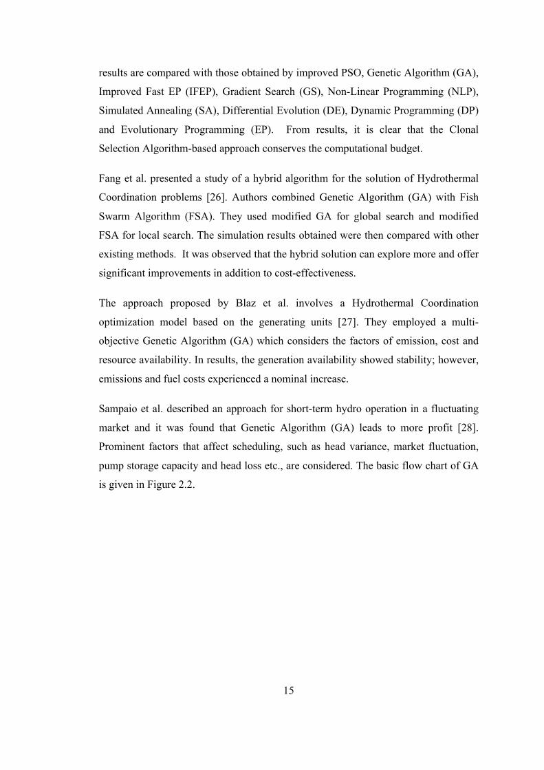
Sampaio et al. described an approach for short-term hydro operation in a fluctuating
market and it was found that Genetic Algorithm (GA) leads to more profit [28].
Prominent factors that affect scheduling, such as head variance, market fluctuation,
pump storage capacity and head loss etc., are considered. The basic flow chart of GA
is given in Figure 2.2.
16
Figure 2.2: Flow chart of Genetic Algorithm (GA)

17
Simoglou et al. analyzed the Greek electricity market for a future period (2014-2020)
[29]. They considered five different energy technologies such as biomass, Solar
Photovoltaic (SPV), wind and Combined Heat and Power (CHP). Simulation results,
done through integrated software tools, signals the viability of large-scale Renewable
Energy System integration.
Behnam et al. considered resolving the self-scheduling issue of risk-constrained
generation system using a nonprobabilistic information gap model based on the
Information Gap Decision Theory [30]. Authors applied their proposed model on a
54-unit thermal generation system and proved that their model is a bit more profitable.
Pousinho et al. presented an MILP-based Approach for a pool based electricity market
and hydropower producer [31]. Authors prove that by adopting their approach
hydropower producers can have 9% more profit as compared to deterministic
approaches.
Koo et al. conducted the load forecasting using two different models [32]. Authors
use k-NN algorithm for load classification of the system. In the research work, they
conclude that Hot Winters have better performance than ARIMA (Autoregressive
Integrated Moving Average).
Batlle et al. presented the techniques for better power expansion planning and
compared them using LEEMA (Low-Emissions Electricity Market Analysis) [33].
Authors considered the thermal cyclic operation costs and proved that startups cost is
also a major factor in generation expansion planning and that it should not be ignored.
Ricardo et al. used Mixed Integer Non-linear Programming (MINLP) and spatial
Hydro Branch & Bound (SHBB) framework for short-term hydro-scheduling of head
dependent systems. Their results demonstrated improvement in performance and
computational time [34].
Tong et al. presented formulation of hydro generation scheduling on the basis of
Mixed Integer Linear Programming (MILP) [35]. Authors considered the linearization
of nonlinear constraints and discussed their impacts. Linearization of tailrace can
make the resulting schedule unacceptable. MILP makes the solution feasible and

18
efficient. Further, it is concluded that real number of water delays can be handled in a
manner ensuring stability of the water balance system.
Gonzalez et al. presented hourly hydrothermal dispatch by using single-node
centralized energy [36]. Authors classify generation technologies. Doing so
accelerates the performance. And, nonlinear constraints, such as elapsed time of
response, ramps, shut down and startup costs etc., are simplified. The proposed model
was applied on a 2010 scenario of Spanish market price. Comparatively better results
were obtained.
Kenneth et al. proposed a model for both demand-side and generation-side
management [37]. On comparing the proposed model with conventional solutions, it
was found able to manage the intermittency issue of Renewable Energy Sources
(RES). Andre Pina et al. presented the framework by using two specific models of
short-term and long-term planning are combined to model Hydrothermal
Coordination [38]. An iterative process is used to combine the results. Significant
reductions in CO2 emissions are observed. However, the model is only productive for
low storage capacity renewable energy systems.
Provas et al. proposed a Quasi-Oppositional Teaching Learning-Based Optimization
(QOTLBO) [39]. Authors used valve point effect and compared the results with the
latest optimization techniques, such as PSO, DE, Modified Differential Evolution
(MDE), Improved Self-adaptive Particle Swarm Optimization (ISAPSO) and neural
network. Findings revealed that the proposed approach had lower trapping chances to
the local minima.
Erlon et al. proposed a model for Hydro Unit Commitment and Loading (HUCL) and
provided the schedule of the day ahead [40]. Authors used an integrated optimization
technique keeping in view cascaded plants. The proposed model complied with the
generation limits and demonstrated improved performance for the basin.
Huifeng et al. presented a new methodology to address the issue of short-term
Hydrothermal Scheduling (HTS) [41]. They considered a heuristic technique and
employed three multi-objective Evolutionary Algorithms. An elitist archive is used to

19
put the non-dominant participants, and this improves the convergence and efficiency,
comparatively though.
Moein et al. solved the Hydrothermal Coordination problem considering the AC
constraints of bus voltages and transmission flow [42]. The methodology is based on
Benders Decomposition method that is improved by Particle Swarm Optimization and
Bacterial Foraging Algorithm. Authors compared the results of Bacterial Foraging
Oriented by Particle Swarm Optimization (BDI-BFPSO), with other techniques, such
as Benders Decomposition Improved by Particle Swarm Optimization (BDI-PSO),
Conventional Benders Decomposition and Benders Decomposition Improved by
Bacterial Foraging Algorithm (BDI-BFA). Their proposed methodology proved to be
effective, in results, but at the cost of trapping in minima. Rui. Zhang et al. considered
the issue of global warming in their Hydrothermal Coordination model [43]. The
proposed solution optimizes the generation system. However, an attempt to reduce
emissions increases in costs of the the generation system.
Javier et al. compared two models i.e. Mixed Integer Non-Linear Programming
(MILP) and Mixed Integer Linear Programming (MILP). The authors applied a non-
linear quadratic function for head and water discharge. It is shown that MINLP is
characterized by greater efficiency and water savings [44].
Xiaohu et al. made use of optimal Economic Dispatch (ED) to estimate risk [45].
Authors used PSO, considering the value at risk, and integrated risk management for
assessing the risk. An optimal tradeoff is approached between the profit and risk for a
hybrid system. It has been concluded that accurate forecasting of wind reduces the
risk.
Xie et al. discussed the issues faced by generation companies while attempting to
integrate wind power plants [46]. They discussed the fundamental problems i.e.
limited predictability and internal temporal variations. It is proposed that under
hazards, operational hurdles can be countered using intelligent computational
techniques.
Costas et al. proposed a self-scheduling hydro production model [47]. Its major aim is
to maximize profit keeping in view the upcoming market trends. Residual demand

20
curve depicts a comparison between the interaction of competitors and load demand.
The curve can be modified to meet the criterion of optimal pumped-hydro bids. To
remove the uncertainty in load demand, water inflow and competitors’ offers,
stochastic multistage programming, based on MILP, is used.
Kamal et al. proposed a Hydrothermal Coordination model based on improved PSO
[48]. Unlike its predecessors, the new PSO did not converge prematurely to a sub-
optimal solution. When compared to Modified Hybrid Differential Evolution
(MHDE) and GA, the proposed solution showed better results.
Cheng et al. proposed a technique based on Progressive Optimality Algorithm (POA)
[49]. Due to high-head real-time operations, short-term scheduling is difficult for
large scale cascaded hydropower plants. Prior to applying optimization, accumulative
mathematical techniques are used to identify forbidden operations zones. The
proposed technique is tested in China, and the results indicated that it can deal with
the complexities of multi-vibration zones.
Ahmad et al. used honey bee algorithm is selected for optimization of multi objective
problem of ED. Cost and emission reduction is done in a competitive market scenario.
Ramp rate limits and valve point loading constraint is considered. The effectiveness
of the algorithm is checked on IEEE standard bus systems of 6 and 10 units
respectively [50].
Basu et al. presented an Artificial Immune System (AIS) for hydrothermal scheduling
of systems comprising of fixed-head hydro systems and thermal systems [51]. Results
obtained from various experiments are compared with existing algorithms such as
Differential Evolution (DE), Evolutionary Programming (EP) and PSO. Numerical
results demonstrated the comparative superiority of AIS.
Senthil et al. discussed various techniques for hydrothermal scheduling [52]. GA
works fine for problems of hydropower plant while lambda iteration method is
preferred for problems relating to thermal power plants. But on considering the line
flow constraints and line losses, GA-based Optimal Power Flow (OPF) proves to be
better for hydrothermal systems. Results show that the GA-based solution minimizes

21
computation time, gives global optimum solution and reduces computational
complexity.
Balasubbareddy et al. used Fruit fly Algorithm and hybridized with Genetic
Algorithm for the power flow problem. They have used the Pareto front for multi-
objective visualization. Fuzzy logic is selected for best selection of best Pareto values.
But it makes system complex and computational budget requirement increases [53].
Frangioni et al. proposed a hybrid sequential approach [54]. Unit Commitment (UC)
is a fundamental problem in short-term electric power generation scheduling system.
The Lagrangian technique is good for lower bounds; however, it needs a new
mathematical model each time. In the same way, MILP offers better results at times
when lower bound is not good. The scheme proposed by the authors, therefore,
combines these two techniques and as a result, a hybrid version proves to be a far
better solution.
Christopher et al. proposed a Simulated Annealing Embedded Evolutionary
Programming (SAEEP) algorithm to solve short-term scheduling problems in power
generation [55]. The solution was able to find the optimum generation schedule and
the less-expensive alternative.
Kanwardeep et al. proposed a novel congestion management solution for thermal and
hydro systems [56]. A piece-wise linearized performance curve is used and to
evaluate effectiveness of the proposed method, authors used the IEEE 118 and IEEE
57 bus systems.
Sivasubramani et al. proposed a hybrid method, combining Sequential Quadratic
Programming (SQP), a global optimizer, and Differential Evolution (DE), a local
optimizer, for the Hydrothermal Coordination problem [57]. Tests are undertaken in a
multi-chain cascaded reservoir system and the proposed method shows its
efficaciousness.
The comprehensive literature review has explored the topic of Hydrothermal
Coordination from multiple dimensions. Further, the pertinent sub-topics, constraints,
objectives and techniques etc., are being summarized as follows.

22
2.3.1 Objectives of Hydrothermal Coordination
From the literature survey of Hydrothermal Coordination, it is observed that primary
concerns that demand attention are the minimization of fuel cost, emission reduction
and maximization of reliability as shown in Figure 2.3.
Cost minimization mainly depends on the selection of fuels i.e. coal is more
economical than natural gas and crude oil. Selection of power plants is also of
importance because the renewable power plants have minimum operational cost as
compared to all fossil fuel power plants. Grid, transmission and distribution system
are also taken into account in cost minimization because the power plants nearby to
load center have minimum losses.
Figure 2.3: Objectives of Hydrothermal Coordination
Regulations by the government also matter in the cost of power generation e.g. a
domestic user can prioritize his usage of electric iron, water pump and washing
machine etc. if peak time extra charges are implemented (Peak Load Pricing). Peak
load pricing regulation decreases the vertical difference between base load and peak
load. Peak load power plants are often more expensive as compared to base load
23
power plants [58]. Competition policy in pump storage and hydro dominated markets
can also decrease the power generation cost. Often, hydro power plants and pump
storage power plants inject more energy during peak time to get maximum benefit due
to which transmission limits and losses of energy come in discussion [59]. So, in short
some of the policies at the national level do matter in the economic dispatch. Clean
environmental regulation (‘implemented by government’) may eliminate the choice of
using coal for power generation even though coal is cheapest, the regulation max
impact the cost of generation.
Reliability maximization is also an objective of HTC that mainly depends on weather
forecasting, fault recognition at the earliest time possible and maintaining the
infrastructure that is aged. Weather prediction is necessary for stable and reliable
hydro operation [60, 61].
Emission minimization is also a key objective of HTC due to the current global
warming and climate change threats. By good selection of fossil fuels, e.g. by
minimizing usage of coal and crude oil, emissions can be minimized. Fuel
consumption can be saved by using cogeneration plants and combined heat plants.
Fuel saving indirectly minimizes the harmful gas emissions [62].
2.3.2 Constraints of Hydrothermal Coordination
In the literature survey, we have observed that there are various constraints which
need to be tackled in case of Hydrothermal Coordination. Some of the most common
constraints are shown in Figure 2.4. Every case study and scenario has its own
combination of constraints and objectives.

24
Figure 2.4: Constraints of Hydrothermal Coordination
2.3.3 Optimization Techniques Applied to Hydrothermal Coordination
From literature, it is evident that researchers follow different approaches to solve the
problem of Hydrothermal Coordination. In the period 1950-1980, classical techniques
were prominent. In the 1990’s, recursive techniques were common and by the end of
20th century Evolutionary Algorithms (EA) dominated the trend. From the start of the
21st century, the trend shifted toward hybrid schemes. Figure 2.5 shows the most
commonly used optimization techniques categorized into the following three major
groups: classical, deterministic and evolutionary.

25
Figure 2.5: Optimization Techniques Applied to Hydrothermal Coordination
2.4 Discussion
Hydro-thermal Scheduling (HTS), or Hydrothermal Coordination, is a highly
complex, non-linear, non-deterministic, multi-constrained and dynamic optimization
problem. Hydrothermal Coordination addresses two major problems i.e. Economic
Dispatch (ED) and Unit Commitment (UC). The solution solves unit selection and
active power dispatch. Search space of Hydrothermal Coordination is non-linear and
very turbulent. Therefore, there is a need for an efficient and robust optimization tool.

26
There are many techniques to solve the Hydrothermal Coordination problem. It has
been observed that conventional approaches are not successful in leading to
acceptable results for a problem that is non-differentiable, non-convex and complex.
The intrinsic complexities and the failure to resolve the challenges have shifted the
pivot to modern intelligent computational techniques, such as nature-inspired
Evolutionary Algorithms (EA). They offer much better outcomes and are open to
further refinement. Intelligent computational techniques, especially Evolutionary
Algorithms, hybridized with conventional techniques are better than classical
techniques.
Hydrothermal Coordination optimization techniques can be classified into three types:
classical, deterministic and evolutionary. Each of the types is characteristic of its pros
and cons. Classical techniques, such as gradient and NR based algorithms, are more
suitable for smooth fuel-cost curves. However, most of the Hydrothermal
Coordination problems have multiple constraints. In case of the non-smooth and
multi-model curve, there are another two options, i.e., deterministic and evolutionary.
The evolutionary option promises the issue redressal in a versatile and reliable
manner.
Compared to other meta-heuristic algorithms, PSO, DE, BFA, and BA are generally
preferred. However, overall, hybrid techniques offer the best results. Differential
evolution falls under the umbrella of deterministic evolutionary algorithm which has
supremacy over the evolutionary algorithms like GA and Swarm based algorithms.
Moreover, physics of the problem is of the quadratic nature and the differential
quadratic performs better as compared to other recursive techniques dynamic and
linear programming.

27
2.5 Chapter Conclusion
The chapter presented a rigorous literature survey of economical hydrothermal
coordination using intelligent computational techniques. HTC objectives have been
identified and discussed. The main objective of HTC is the economical operation of
hydro and thermal power plants by effective utilization of the available options. Later
on, HTC constraints are presented that are to be fulfilled. The main constraint of HTC
is that the power generation should be equal to the power demand by considering
transmission losses. In the end, the recent developments in ICT, with their pros and
cons, are discussed keeping in mind the classical, recursive and evolutionary
techniques.

28
3 Power Plants Development Trend

29
3.1 Chapter Summary
The chapter presents a comprehensive study about alternatives in power generation.
Levelized Cost of Electricity (LCOE) is discussed for coming forth with the best
solution. Existing models are compared along with their pros and cons. Finally, a
discussion is made about the suitability of a power plant in different conditions and
scenarios. It has been observed that per annum global electricity generation has
increased from 19.1 to 24.2 Petawatt hour. Similarly, CO2 emission has increased
from 10.5 to 12.9 Gigaton annually.
3.2 Background
In today’s rapidly digitizing global village, electricity demand is increasing owing to
rapid industrialization and modernized living standards. Therefore, electric power
generation and its development receive a significant portion of the national exchequer.
Utilizing a hybrid power generation mechanism and ensuring its optimal operation is
complex and tedious owing to various factors. Some of such factors include nature of
energy resource, availability, emissions, reliability, costs incurred and budget
constraints etc.
Electricity is one of the greatest blessings of science. There are many options for
power generation, each with its advantages and disadvantages. The selection criterion
varies owing to differences in environment, area and situation etc. [63, 64].
Availability of different sources enhances the reliability of the power system,
indirectly though. Source selection depends on the distance between load and
generation site. The density of the consumer population also influences the choice of
source selection [65]. Involving more selection considerations can further increase the
overall cost of the system. Due to high gains, wise selection of energy sources and
judicious component-sizing is mandatory so as to minimize the system costs and other
relevant expenses [66].
Supply Side Management (SSM) is a terminology that deals with clean generation of
electricity with reliability and cost-effective manner [67]. There are two main types of
30
sources: non-renewable and renewable. Most economical energy option is to be
considered, as the basic criterion [68, 69].
There is a significant portion of literature dedicated to demand side management and
distribution management; however, generation management has received little
attention [70]. Therefore, it is important to consider the issue of generation
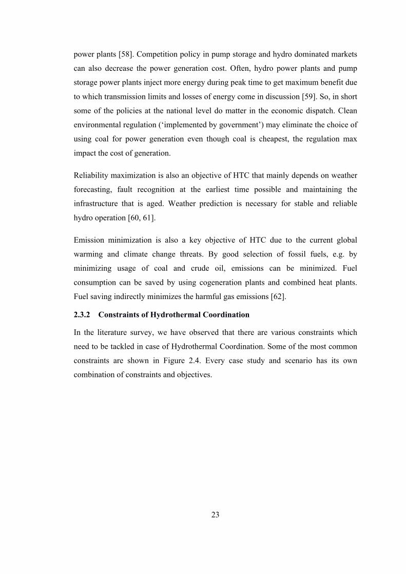
management. It will significantly reduce costs. Major renewable energy sources
include hydropower, solar energy, wind energy, geothermal energy, tidal and
biomass. Non-renewable sources of energy are coal, oil and natural gas. Figure 3.1
depicts some of the major types of the power generation system.
Figure 3.1: Types of power generation systems with respect to the energy source
A power plant has various associated costs. In addition, there are concerns about
emission and reliability. Normally, parameters such as capital cost and operation cost
are used to choose the appropriate power plant in a given situation [71]. Levelized
Cost Of Electricity (LCOE) is the sum of capital, operation, and maintenance costs
divided by total energy produced in a power plant’s lifetime, keeping in view the

31
capacity factor [72, 73]. Calculating LCOE is an important step in order to select the
most suitable energy option [70]. In the literature, techniques dealing with costs of
power generation consider either economical cost, emission concerns and/or
reliability. There is little research work that considers LCOE.
Green House Gas (GHG) emission is the largest contributor to global warming [74].
According to the International Energy Agency (IEA), by 2040, premature deaths will
increase from 3 million to 4 million and CO2 emission rates will increase by 5% [75].
The situation is deteriorating, and it signals further urgent remedial actions. Present
era scientists, engineers and policymakers need to come forward with practical
solutions. One of the solutions to address the issue of GHG emission is the carbon tax,
a tax levied on the establishments that emit GHG’s. Solid implementation of suchlike
policy can result in the dominance of green technologies [76, 77].
During the last decade, a major chunk of the world’s energy demand came from
China and India. About one-third of the world’s population resides in India and China
[78, 79]. Coal has a major share in their energy generation mix [71]. Recently,
because of climate-friendly international policy endeavors, renewable energy
technologies are receiving attention worldwide [71, 72]. For instance, Germany and
Denmark are at the forefront of considering eco-friendly energy solutions [73].
On the other hand, the United States is investing more on coal and gas-based energy
solutions. US is one of the major suppliers of LNG and fossil fuels after Saudi Arabia,
Iran and Iraq [80].
3.3 Levelized Cost of Electricity (LCOE)
Levelized Cost of Electricity (LCOE) is an approximation of the average price of
a generating station for its lifetime. It is obtained by dividing the life-cycle cost of the
generation source by life-time energy produced, called Levelized Energy Cost (LEC)
[81]. It is also construed as a measure of the overall competitiveness of different
generation sources. The list of inputs required to calculate LCOE includes the
following: fuel cost, capital cost, fixed cost, variable maintenance cost, financing cost,
operational cost and an assumed duty rate for power plant technologies [72]. Fuel cost
32
is nearly negligible in the case of wind and solar power generation technologies.
Operation and maintenance expenses are also relatively less. Therefore, for wind and
solar energy, LCOE, to a large extent, depends on the capital cost of the power plant
[82].
The Levelized Avoided Cost of Electricity (LACE) is cited as another measure of the
overall competitiveness amongst different power generation sources. It measures the
annual economic value of the potential power generating project [83]. Since LACE
depends, to a larger extent, on local geographic variables, it is not that appropriate in
the global context [84]. Keeping in view a power plant’s financial life and utilization
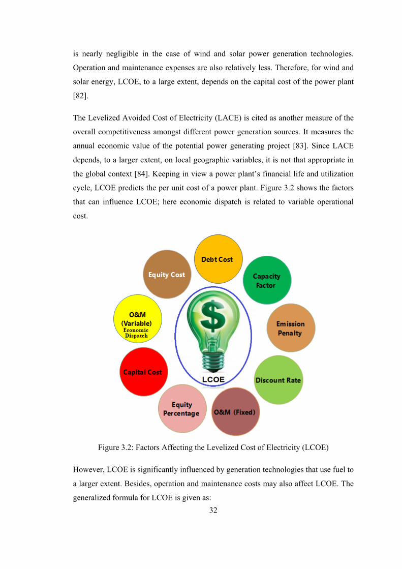
cycle, LCOE predicts the per unit cost of a power plant. Figure 3.2 shows the factors
that can influence LCOE; here economic dispatch is related to variable operational
cost.
Figure 3.2: Factors Affecting the Levelized Cost of Electricity (LCOE)
However, LCOE is significantly influenced by generation technologies that use fuel to
a larger extent. Besides, operation and maintenance costs may also affect LCOE. The
generalized formula for LCOE is given as:

33
(3.1)
In the case of nuclear and non-renewable sources of energy, LCOE has remained
nearly unvaried in the last decade [85, 86]. However, solar energy has experienced a
shift in LCOE by up to 75%.
Among the renewable energy sources, hydropower has the least cost (Figure. 3.3)
followed by wind energy and Solar Photovoltaic (SPV) energy [85, 87, 88]. There are,
however, some issues linked with hydropower, as it involves mass public
displacement, and wind energy, since it is not available during peak load time.
Figure 3.3: Global Levelized Cost of Electricity (LCOE) of Power Generation in 2017
3.3.1 Non-Renewable Energy Sources
About half of world’s electricity demands are met by fossil fuels. Thermal power
plants generate energy from coal, oil, gas and nuclear. Heat is transferred in either of
the three ways i.e. conduction, convection and radiation. Thermal power plants utilize
the steam thrust to move the generation wheel. Two major costs are involved in a
LCOE =Cc − Σt=1
Lc dsΨ t ×Θ + Σt=1LcOcΨ
t × (1−Θ)− SvΨLc
Γ Σt=1LcΨ t × SDt
$-
$0.05
$0.10
$0.15
$0.20
$0.25
Concentra
ting S
olar
Ofshore W
ind
Solar
Photovolta
ic
Geothermal
Biomass
Onshore W
indHyd
ro
Fossi
l Fuels
$0.22
$0.14
$0.10
$0.07 $0.07 $0.06 $0.05
$0.10
Global LCOE of Power Generation-2017 (US$/kWh)

34
thermal power plant: capital cost and operational cost, with both of them depending
on fuel price [89].
3.3.1.1 Electricity Generation by Coal
Coal power plants dominate the energy scenario. In the last decade alone, coal
produced about one-third of electricity on annual basis [90-101]. One of the major
reasons behind preferring coal is its comparatively lower costs. However, the
environmental costs are generally ignored. Normally, electricity is generated by coal
at a smaller scale; however, if used at a larger scale, coal proves to be a useful and
cost-effective option. Coal does come with a drawback i.e. GHG emissions, which are
harmful to health and environment.
Since coal-fired power plants have been used since long, its technology has attained
maturity. To further complement, coal is available widely and is cheap,
comparatively. Coal plants are installed at places where coal is abundant. Adoption of
coal is increasing in Asia Pacific while the case is vice versa in Europe. Figure 3.4
shows the penetration of coal that has increased by 25% in the last decade.
Figure 3.4: Trend of coal-based electricity generation (2008-2017)
3.3.1.2 Electricity Generation by Oil
During the first decade of the 20th century, oil as an energy source received large
attention. Events such as Arab oil embargo of the 1970’s and the concerns behind its
0.00 2.00 4.00 6.00 8.00 10.00 12.00
2008200920102011201220132014201520162017
Electricity (PWh)
Year
Net Electricity Generation (Coal)
25%

35
limited supply shifted the attention toward natural gas. Cost of fuel has a pivotal role
to play in ascertaining the power generated from petroleum sources. For instance, as
per Figure 3.5, generation from liquid fuels decreased by about 20% in the last decade
[90-99].
Figure 3.5: Trend of global electricity generation by oil (2008-2017)
3.3.1.3 Electricity Generation by Gas
After coal comes the natural gas fired power plants as they are widely used. Gas can
be easily transported across the borders and is economical. Therefore, it is preferred
over liquid fuels. Such power plants have lower capital costs and can be used as peak
power plants because of lesser startup time. Natural gas power plants grew by about
1/3rd in the last decade (Fig 3.6) [90-99].
0 0.2 0.4 0.6 0.8 1 1.2
2008200920102011201220132014201520162017
Electricity (PWh)
Year
Net Electricity Generation (Oil)
-18%
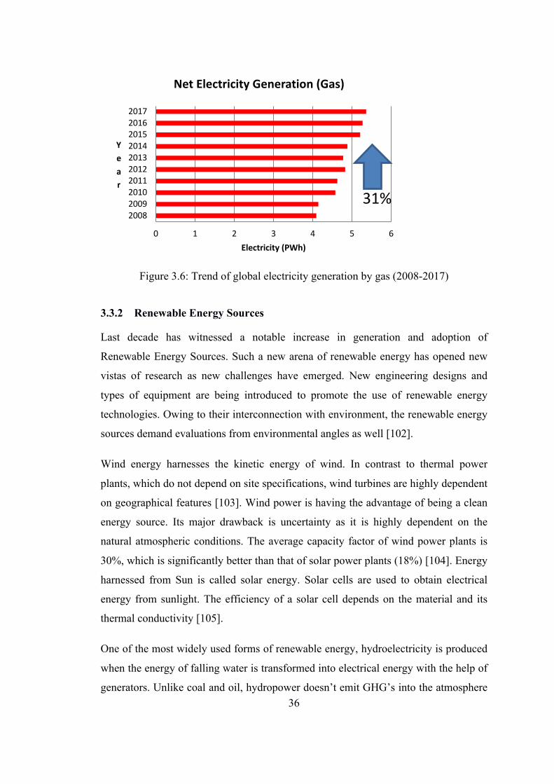
36
Figure 3.6: Trend of global electricity generation by gas (2008-2017)
3.3.2 Renewable Energy Sources
Last decade has witnessed a notable increase in generation and adoption of
Renewable Energy Sources. Such a new arena of renewable energy has opened new
vistas of research as new challenges have emerged. New engineering designs and
types of equipment are being introduced to promote the use of renewable energy
technologies. Owing to their interconnection with environment, the renewable energy
sources demand evaluations from environmental angles as well [102].
Wind energy harnesses the kinetic energy of wind. In contrast to thermal power
plants, which do not depend on site specifications, wind turbines are highly dependent
on geographical features [103]. Wind power is having the advantage of being a clean
energy source. Its major drawback is uncertainty as it is highly dependent on the
natural atmospheric conditions. The average capacity factor of wind power plants is
30%, which is significantly better than that of solar power plants (18%) [104]. Energy
harnessed from Sun is called solar energy. Solar cells are used to obtain electrical
energy from sunlight. The efficiency of a solar cell depends on the material and its
thermal conductivity [105].
One of the most widely used forms of renewable energy, hydroelectricity is produced
when the energy of falling water is transformed into electrical energy with the help of
generators. Unlike coal and oil, hydropower doesn’t emit GHG’s into the atmosphere
0 1 2 3 4 5 6
2008200920102011201220132014201520162017
Electricity (PWh)
Year
Net Electricity Generation (Gas)
31%

37
[106]. Hydropower generation has experienced a growth of about 25% in the last
decade (Figure 3.7) [90-99].
Figure 3.7: Trend of hydel generation in the world in the last decade
3.3.2.1 Geothermal Energy
Geothermal energy involves obtaining heat energy from the core of the earth. A
geothermal power plant can be thought of as a modified version of a thermal power
plant. While a thermal plant has a boiler and a burning fuel, the geothermal
counterpart does not demand such elements. In geothermal energy, the heat trapped
underground is made into use by rock catchers and injection wells [107]. Two types
of geothermal plants are being used worldwide: dry-steam plants-and flash-steam
plants. Flash steam power plants are younger as compared to dry steam. The use of
geothermal energy dates back to the 20th century; however, due to lower efficiency it
couldn’t progress then. In the last decade use of geothermal energy has increased by
almost 25% [90-99].
0 1 2 3 4 5
2008200920102011201220132014201520162017
Electricity (PWh)
Year
Net Electricity Generation (Hydro)
24%
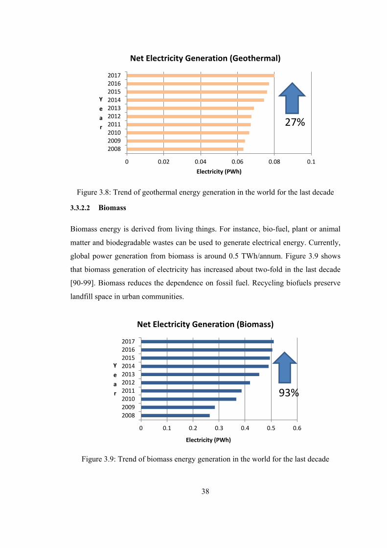
38
Figure 3.8: Trend of geothermal energy generation in the world for the last decade
3.3.2.2 Biomass
Biomass energy is derived from living things. For instance, bio-fuel, plant or animal
matter and biodegradable wastes can be used to generate electrical energy. Currently,
global power generation from biomass is around 0.5 TWh/annum. Figure 3.9 shows
that biomass generation of electricity has increased about two-fold in the last decade
[90-99]. Biomass reduces the dependence on fossil fuel. Recycling biofuels preserve
landfill space in urban communities.
Figure 3.9: Trend of biomass energy generation in the world for the last decade
0 0.02 0.04 0.06 0.08 0.1
2008200920102011201220132014201520162017
Electricity (PWh)
Year
Net Electricity Generation (Geothermal)
27%
0 0.1 0.2 0.3 0.4 0.5 0.6
2008200920102011201220132014201520162017
Electricity (PWh)
Year
Net Electricity Generation (Biomass)
93%
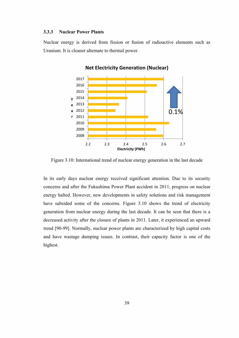
39
3.3.3 Nuclear Power Plants
Nuclear energy is derived from fission or fusion of radioactive elements such as
Uranium. It is cleaner alternate to thermal power.
Figure 3.10: International trend of nuclear energy generation in the last decade
In its early days nuclear energy received significant attention. Due to its security
concerns and after the Fukushima Power Plant accident in 2011, progress on nuclear
energy halted. However, new developments in safety solutions and risk management
have subsided some of the concerns. Figure 3.10 shows the trend of electricity
generation from nuclear energy during the last decade. It can be seen that there is a
decreased activity after the closure of plants in 2011. Later, it experienced an upward
trend [90-99]. Normally, nuclear power plants are characterized by high capital costs
and have wastage dumping issues. In contrast, their capacity factor is one of the
highest.
2.2 2.3 2.4 2.5 2.6 2.7
2008200920102011201220132014201520162017
Electricity (PWh)
Year
Net Electricity Generation (Nuclear)
0.1%
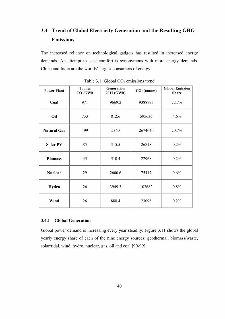
40
3.4 Trend of Global Electricity Generation and the Resulting GHG
Emissions
The increased reliance on technological gadgets has resulted in increased energy
demands. An attempt to seek comfort is synonymous with more energy demands.
China and India are the worlds’ largest consumers of energy.
Table 3.1: Global CO2 emissions trend
Power Plant Tonnes CO2/GWh
Generation 2017 (GWh) CO2 (tonnes) Global Emission
Share
Coal 971 9669.2 9388793 72.7%
Oil 733 812.6 595636 4.6%
Natural Gas 499 5360 2674640 20.7%
Solar PV 85 315.5 26818 0.2%
Biomass 45 510.4 22968 0.2%
Nuclear 29 2600.6 75417 0.6%
Hydro 26 3949.3 102682 0.8%
Wind 26 888.4 23098 0.2%
3.4.1 Global Generation
Global power demand is increasing every year steadily. Figure 3.11 shows the global
yearly energy share of each of the nine energy sources: geothermal, biomass/waste,
solar/tidal, wind, hydro, nuclear, gas, oil and coal [90-99].

41
Figure 3.11: Global electricity generation trend observed in the last decade
Furthermore, we reviewed the policies taken by G20 members regarding allocation of
resources for power generation. The reason for taking information of G20 members is
because collectively they account for about 85% of the global economy as well as
housing about 67% of the world’s population and 4/5 of the world trade. Thus they
are considered to be the most successful countries in terms of economic policies and
so their economic policies should be set as examples for other developing or
underdeveloped countries. This is the reason why we chose these countries as
examples for our study into how they chose indigenous resources, indigenous
technology and cheap resources for minimization of costs.
The most prominent example is the Kingdom Of Saudi Arabia. In Saudi Arabia,
Almost 70 percent of energy power plants use Gas while the rest of them use oil as
their primary source of energy. This is because Oil and Gas are the indigenous
resource for Saudi Arabia hence proving that for efficient allocation of resources for
energy production and cost minimization, countries should use resources readily
available to them.
0
5000
10000
15000
20000
25000
2008 2009 2010 2011 2012 2013 2014 2015 2016 2017 Cost2010
Tera
Wh
Year
Net Global Generation Geothermal
Biomass/Waste
Solar/Tidal
Wind
Hydro
Nuclear
Gas
Oil
Coal
26%
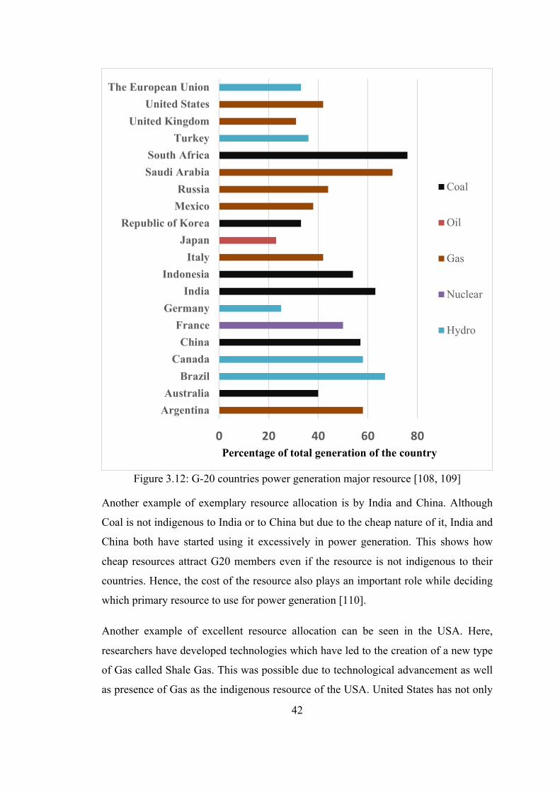
42
Figure 3.12: G-20 countries power generation major resource [108, 109]
Another example of exemplary resource allocation is by India and China. Although
Coal is not indigenous to India or to China but due to the cheap nature of it, India and
China both have started using it excessively in power generation. This shows how
cheap resources attract G20 members even if the resource is not indigenous to their
countries. Hence, the cost of the resource also plays an important role while deciding
which primary resource to use for power generation [110].
Another example of excellent resource allocation can be seen in the USA. Here,
researchers have developed technologies which have led to the creation of a new type
of Gas called Shale Gas. This was possible due to technological advancement as well
as presence of Gas as the indigenous resource of the USA. United States has not only
0 20 40 60 80
ArgentinaAustralia
BrazilCanada ChinaFrance
GermanyIndia
IndonesiaItaly
JapanRepublic of Korea
MexicoRussia
Saudi ArabiaSouth Africa
TurkeyUnited Kingdom
United StatesThe European Union
Percentage of total generation of the country
Coal
Oil
Gas
Nuclear
Hydro
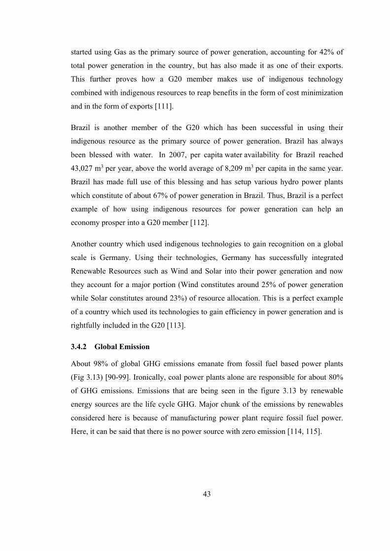
43
started using Gas as the primary source of power generation, accounting for 42% of
total power generation in the country, but has also made it as one of their exports.
This further proves how a G20 member makes use of indigenous technology
combined with indigenous resources to reap benefits in the form of cost minimization
and in the form of exports [111].
Brazil is another member of the G20 which has been successful in using their
indigenous resource as the primary source of power generation. Brazil has always
been blessed with water. In 2007, per capita water availability for Brazil reached
43,027 m3 per year, above the world average of 8,209 m3 per capita in the same year.
Brazil has made full use of this blessing and has setup various hydro power plants
which constitute of about 67% of power generation in Brazil. Thus, Brazil is a perfect
example of how using indigenous resources for power generation can help an
economy prosper into a G20 member [112].
Another country which used indigenous technologies to gain recognition on a global
scale is Germany. Using their technologies, Germany has successfully integrated
Renewable Resources such as Wind and Solar into their power generation and now
they account for a major portion (Wind constitutes around 25% of power generation
while Solar constitutes around 23%) of resource allocation. This is a perfect example
of a country which used its technologies to gain efficiency in power generation and is
rightfully included in the G20 [113].
3.4.2 Global Emission
About 98% of global GHG emissions emanate from fossil fuel based power plants
(Fig 3.13) [90-99]. Ironically, coal power plants alone are responsible for about 80%
of GHG emissions. Emissions that are being seen in the figure 3.13 by renewable
energy sources are the life cycle GHG. Major chunk of the emissions by renewables
considered here is because of manufacturing power plant require fossil fuel power.
Here, it can be said that there is no power source with zero emission [114, 115].

44
Figure 3.13: Percentage emission in the world by different power sources in 2017
Owing to severity of the issue (Figure 3.13), an emission control strategy is proposed.
3.5 Discussion
Global power generation is increasing. In the last decade alone, the annual growth met
557 Terawatt hours (TWh). With the same trend, it would double by 2045. One of the
major key findings of the study is that the trend of international power generation
growth is related to Levelized Cost Of Electricity (LCOE) and emission reduction.
LCOE of renewable energy sources, especially Solar Photovoltaic (SPV) and
Offshore Wind Energy is decreasing rapidly.
3.5.1 Cost
Power plants running on indigenous resources of energy are a far better option,
comparatively, as they are economical and are easily maintained. Transmission costs
constitute a significant portion of overall expenses in the case of centralized grids.
Solar power plants, on the other hand, save such transmission costs to a larger extent.
3.5.2 Emission
Renewable energy power plants should be preferred to conventional fossil-fuel energy
sources. Ignoring the renewable energy options will entail extra costs for emission
0.0%
20.0%
40.0%
60.0%
80.0%
100.0%
Coal Oil NaturalGas
Solar PV Biomass Nuclear Hydro Wind
72.7%
4.6%
20.7%
0.2% 0.2% 0.6% 0.8% 0.2%
Global CO2 Emission of Power Plants (2017)

45
reductions. Besides, carbon pricing, which also promises transition to renewable
energy options, will also enable the governments to accumulate huge revenue.
3.5.3 Reliability
On a general note, non-renewable energy options are considered more reliable than
renewable energy options. However, they come with additional drawbacks such as
GHG emissions and social costs. A diversified energy mix should be preferred
instead. Adding power storage mechanisms such as pump storage and compressed air
to renewable energy plants can make it more reliable.
3.5.4 Global Emission Control Strategy
Carbon emissions can be controlled if the stakeholders adopt a three-pronged
approach:
• Climate Finance
There are, currently, many governmental programs which dedicate subsidies
for fossil fuel power plants. Suchlike subsidies should be withdrawn
immediately. Instead, initiatives providing subsidies to renewable energy
plants should be encouraged. In doing so, phase-out compensation for fossil
fuel power plants should be paid by the respective governments.
• Carbon Pricing
Imposing a carbon tax can encourage the adoption of renewable energy
sources. It also decreases GHG emissions. For a consumer, the carbon tax will
serve either of the two purposes: enable a transition to renewable energy or
encourage the innovation of emission-free alternates.
• Domestic Policies
In addition to national and global levels, policies for encouraging eco-friendly
initiative should be adopted on domestic scale as well. City governments and
municipal establishments should play an integral part. This will enhance skill
development and entrepreneurship in the area of energy.
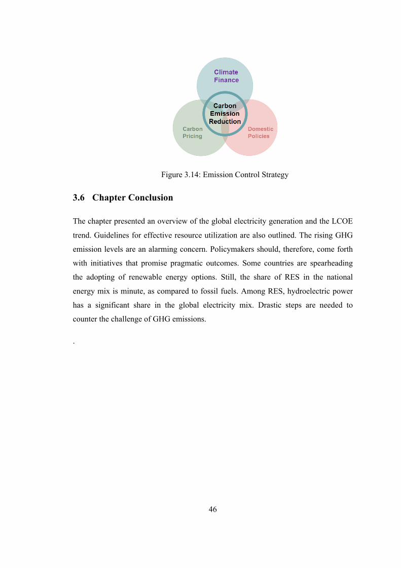
46
Figure 3.14: Emission Control Strategy
3.6 Chapter Conclusion
The chapter presented an overview of the global electricity generation and the LCOE
trend. Guidelines for effective resource utilization are also outlined. The rising GHG
emission levels are an alarming concern. Policymakers should, therefore, come forth
with initiatives that promise pragmatic outcomes. Some countries are spearheading
the adopting of renewable energy options. Still, the share of RES in the national
energy mix is minute, as compared to fossil fuels. Among RES, hydroelectric power
has a significant share in the global electricity mix. Drastic steps are needed to
counter the challenge of GHG emissions.
.

47
4 Long-Term Hydrothermal Coordination (LTHTC)
48
4.1 Chapter Summary
The chapter addresses Long-term Hydrothermal Coordination (LTHTC), which deals
with durations lasting from 1 week to 1 year. Forecasting the resource and addressing
the complexity are two of the main focuses of this chapter. Primary objectives are cost
minimization and emission reduction. A case study about a local power project is
considered for investigation purposes. For forecasting, Markov Chain, a stochastic
prediction model, is used. Intelligent computation for the optimal trade-off is carried
out by Particle Swarm Optimization (PSO).
4.2 Background
Worldwide, a major portion of electricity demand is met by hydroelectric and thermal
power projects. One of the emerging challenges is to devise a coordination
mechanism between these two sources. Such coordination leads to maximum
efficiency. Secondly, fossil fuel is a finite resource. Introducing Economic Dispatch
(ED) can reduce fuel consumption. Rising emission levels is another issue. GHG’s
emitted from thermal power plants, such as CO2, NO2 and SO2 etc, have caused
environmental problems such as ozone depletion, acid rain and rising temperature.
Emissions can be reduced by adopting eco-friendly energy options. Hydropower
plants can provide energy on larger scales in an eco-friendly manner. Hydropower
plants are, therefore, one of the best alternates.
Predicting the potential of water is not deterministic or understood in advance. Rather,
it is stochastic and remains variable. Finite nature of fossil-fuel and the associated
environmental hazards have encouraged the adoption of clean energy. Solar and wind
energy is gaining acceptance from the public. Here, Markov Chain method is used to
ensure maximum utilization from the stochastic nature of hydropower. This method is
important as it can truly predict the stochastic nature of hydropower for intended
outcomes. Moreover, Particle Swarm Optimization (PSO) technique has been used.
The primary objective of the chapter is to aim for a solution that is economical and
possess minimal environmental costs. One of the proposed solutions uses a
combination of the hydropower plant, for providing base load, and other energy
options, such as thermal plant and renewable energy, for the rest of the load. The
49
results were finalized using the following strategies: Economic Load Dispatch,
Economic Emission Dispatch and Combined Load and Emission Dispatch.
4.3 Electricity Sector in Pakistan
Pakistan is a South Asian country and so has a developing economy. This developing
economy has given rise to industries around the country which has further led to the
creation of demand for electricity. Being a developing country, Pakistan is not a
stranger to high birth rates which is a major reason for the increasing population of
the country. This increase in population has further led to increase in domestic
demand for electricity which is another problem for the country. Due to the huge
influx of new industries and the increasing population of a developing country,
Pakistan has still not been able to meet the demand for electricity in the country and
the supply demand gap for electricity has touched 7 GW in the past years.
Pakistan is blessed with 5 Rivers including River Indus which has more volume of
water than River Nile. Due to these resources, Pakistan makes around 99 percent of its
electricity by Hydro and Thermal Power Plants (Pakistan Energy Year Book 2017).
Pakistan has 4 major Hydro Power Plants i.e. Tarbela, Ghazi-Barotha, Mangla and
Neelum Jhelum. From these 4, we have selected Ghazi-Barotha as our case study for
this chapter.
4.4 System Model and Problem Formulation
Hydropower generation depends on water inflow, which is susceptible to seasonal
variations. Therefore, simultaneously scheduling thermal generating units and
ensuring control of GHG emissions is one of the major challenges. Using Particle
Swarm Optimization on a monthly basis can help solve the problem.
4.4.1 Hydropower Power Plant and Load Demand
Hydropower plants occupy a major share in modern power systems. They offer
affordable and clean energy with minimum operational costs. For analysis purposes, a
local site of Ghazi Barotha, Pakistan has been taken into consideration. Historical data
about water inflow and average energy demand of Khyber Pakhtoonkhwa (KP)

50
province is obtained from repositories of Water and Power Development Authority
(WAPDA) (Table 4.1) [116]. Table 4.2 shows the monthly average load demand of
Khyber Pakhtunkhwa (KP).
Table 4.1: Average monthly inflow of Ghazi Barotha site from 2010 to 2017 in Cumecs
Jan Feb Mar Apr May Jun Jul Aug Sep Oct Nov Dec
2010 856 950 1100 1600 1600 1600 1600 1560 1510 1550 1220 600
2011 1200 1066 870 1580 1600 1700 1600 1600 1327 1300 1150 605
2012 1400 688 831 1300 1600 1600 1620 1580 1580 1520 922 580
2013 1300 800 1100 1200 1600 1620 1650 1700 1500 1300 1000 700
2014 1235 1000 750 1250 1600 1600 1675 1600 1493 1500 1000 720
2015 1000 700 600 1470 1675 1700 1700 1600 1140 950 860 800
2016 434 1061 831 1065 1622 1606 1649 1607 1571 1380 1516 980
2017 245 871 720 957 1600 1615 1661 1683 1701 1348 1240 707
The dominant challenge lies in predicting the water inflow, because of its randomly
probabilistic behavior. Therefore, previous year inflow data was essential to predict
the next year’s inflow.
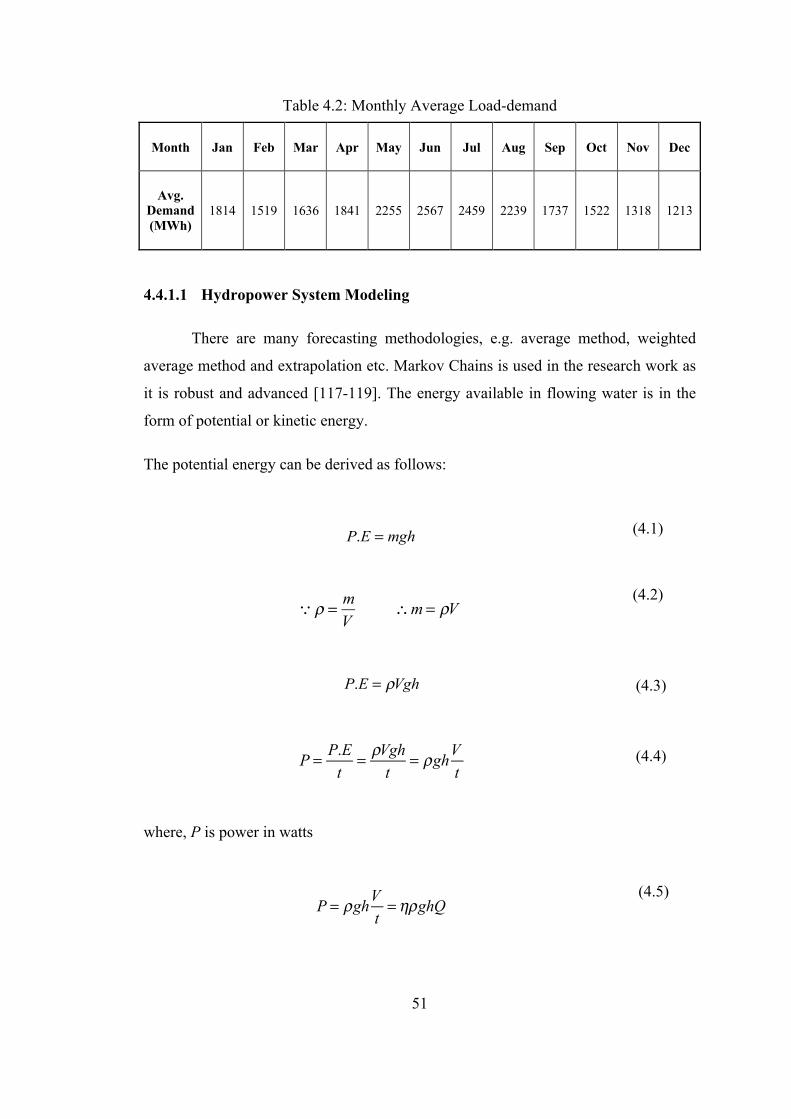
51
Table 4.2: Monthly Average Load-demand
Month Jan Feb Mar Apr May Jun Jul Aug Sep Oct Nov Dec
Avg. Demand (MWh)
1814 1519 1636 1841 2255 2567 2459 2239 1737 1522 1318 1213
4.4.1.1 Hydropower System Modeling
There are many forecasting methodologies, e.g. average method, weighted
average method and extrapolation etc. Markov Chains is used in the research work as
it is robust and advanced [117-119]. The energy available in flowing water is in the
form of potential or kinetic energy.
The potential energy can be derived as follows:
(4.1)
(4.2)
(4.3)
(4.4)
where, P is power in watts
(4.5)
P.E = mgh
Qρ = mV
∴m = ρV
P.E = ρVgh
P = P.Et
= ρVght
= ρghVt
P = ρghVt=ηρghQ
52
And, in case of flowing/running water, the energy of water is kinetic
energy (KE), which can be expressed mathematically as:
(4.6)
(4.7)
where, the variables ρ, A, v, and V denote water density (kg/m3), area (m2), the
velocity of water flow (m/sec) and volume of flowing water (m3) respectively.
(4.8)
(4.9)
where, water density is in kg/m3 (1000 kg/m3), water discharge in m3/sec and
acceleration due to gravity in m/sec2.
From Equation 4.9, it can be inferred that power is directly proportional to flow rate,
cross-sectional area, density of water and efficiency.
4.4.1.2 Stream-inflow and Markov Chain
Markov chain is one of the most popular and accurate methods for forecasting the
water inflow. It is a stochastic procedure which makes use of possible scenarios and
recurrent patterns in order to forecast the current event.
Markov chain can be mathematically expressed as,
K .E = 12mv2
K .E = 12ρAxv2
P = K .Et
= 12ρAxv2
t= 1
2ρA xtv2 = 1
2ρAvv2
P = 12ηρAv3
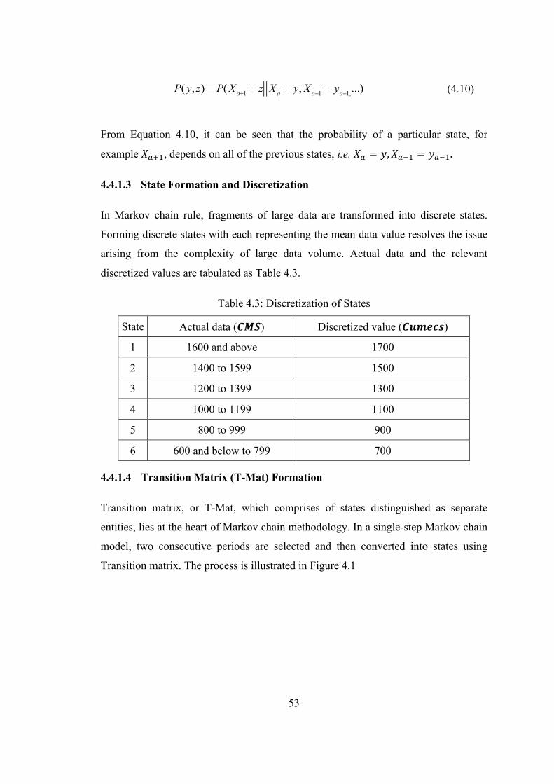
53
(4.10)
From Equation 4.10, it can be seen that the probability of a particular state, for
example 𝑋"#$, depends on all of the previous states, i.e. 𝑋" = 𝑦, 𝑋"($ = 𝑦"($.
4.4.1.3 State Formation and Discretization
In Markov chain rule, fragments of large data are transformed into discrete states.
Forming discrete states with each representing the mean data value resolves the issue
arising from the complexity of large data volume. Actual data and the relevant
discretized values are tabulated as Table 4.3.
Table 4.3: Discretization of States
State Actual data (𝑪𝑴𝑺) Discretized value (𝑪𝒖𝒎𝒆𝒄𝒔)
1 1600 and above 1700
2 1400 to 1599 1500
3 1200 to 1399 1300
4 1000 to 1199 1100
5 800 to 999 900
6 600 and below to 799 700
4.4.1.4 Transition Matrix (T-Mat) Formation
Transition matrix, or T-Mat, which comprises of states distinguished as separate
entities, lies at the heart of Markov chain methodology. In a single-step Markov chain
model, two consecutive periods are selected and then converted into states using
Transition matrix. The process is illustrated in Figure 4.1
P( y, z) = P(Xa+1 = z Xa = y,Xa−1 = ya−1,...)

54
January
February
March
April
May
June
July
August
September
October
November
December
Figure 4.1: State diagrams of the period January to December
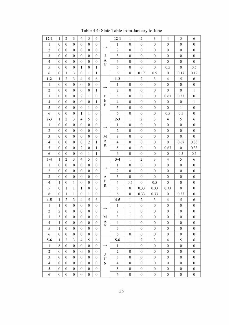
55
Table 4.4: State Table from January to June
12-1 1 2 3 4 5 6
→ J A N
12-1 1 2 3 4 5 6 1 0 0 0 0 0 0 1 0 0 0 0 0 0 2 0 0 0 0 0 0 2 0 0 0 0 0 0 3 0 0 0 0 0 0 3 0 0 0 0 0 0 4 0 0 0 0 0 0 4 0 0 0 0 0 0 5 0 0 0 1 0 1 5 0 0 0 0.5 0 0.5 6 0 1 3 0 1 1 6 0 0.17 0.5 0 0.17 0.17
1-2 1 2 3 4 5 6
→
F E B
1-2 1 2 3 4 5 6 1 0 0 0 0 0 0 1 0 0 0 0 0 0 2 0 0 0 0 0 1 2 0 0 0 0 0 1 3 0 0 0 2 1 0 3 0 0 0 0.67 0.33 0 4 0 0 0 0 0 1 4 0 0 0 0 0 1 5 0 0 0 0 1 0 5 0 0 0 0 1 0 6 0 0 0 1 1 0 6 0 0 0 0.5 0.5 0
2-3 1 2 3 4 5 6
→
M A R
2-3 1 2 3 4 5 6 1 0 0 0 0 0 0 1 0 0 0 0 0 0 2 0 0 0 0 0 0 2 0 0 0 0 0 0 3 0 0 0 0 0 0 3 0 0 0 0 0 0 4 0 0 0 0 2 1 4 0 0 0 0 0.67 0.33 5 0 0 0 2 0 1 5 0 0 0 0.67 0 0.33 6 0 0 0 0 1 1 6 0 0 0 0 0.5 0.5
3-4 1 2 3 4 5 6
→
A P R
3-4 1 2 3 4 5 6 1 0 0 0 0 0 0 1 0 0 0 0 0 0 2 0 0 0 0 0 0 2 0 0 0 0 0 0 3 0 0 0 0 0 0 3 0 0 0 0 0 0 4 1 0 1 0 0 0 4 0.5 0 0.5 0 0 0 5 0 1 1 1 0 0 5 0 0.33 0.33 0.33 0 0 6 0 1 1 0 1 0 6 0 0.33 0.33 0 0.33 0
4-5 1 2 3 4 5 6
→
M A Y
4-5 1 2 3 4 5 6 1 1 0 0 0 0 0 1 1 0 0 0 0 0 2 2 0 0 0 0 0 2 1 0 0 0 0 0 3 3 0 0 0 0 0 3 1 0 0 0 0 0 4 1 0 0 0 0 0 4 1 0 0 0 0 0 5 1 0 0 0 0 0 5 1 0 0 0 0 0 6 0 0 0 0 0 0 6 0 0 0 0 0 0
5-6 1 2 3 4 5 6 → J U N
5-6 1 2 3 4 5 6 1 8 0 0 0 0 0 1 1 0 0 0 0 0 2 0 0 0 0 0 0 2 0 0 0 0 0 0 3 0 0 0 0 0 0 3 0 0 0 0 0 0 4 0 0 0 0 0 0 4 0 0 0 0 0 0 5 0 0 0 0 0 0 5 0 0 0 0 0 0 6 0 0 0 0 0 0 6 0 0 0 0 0 0
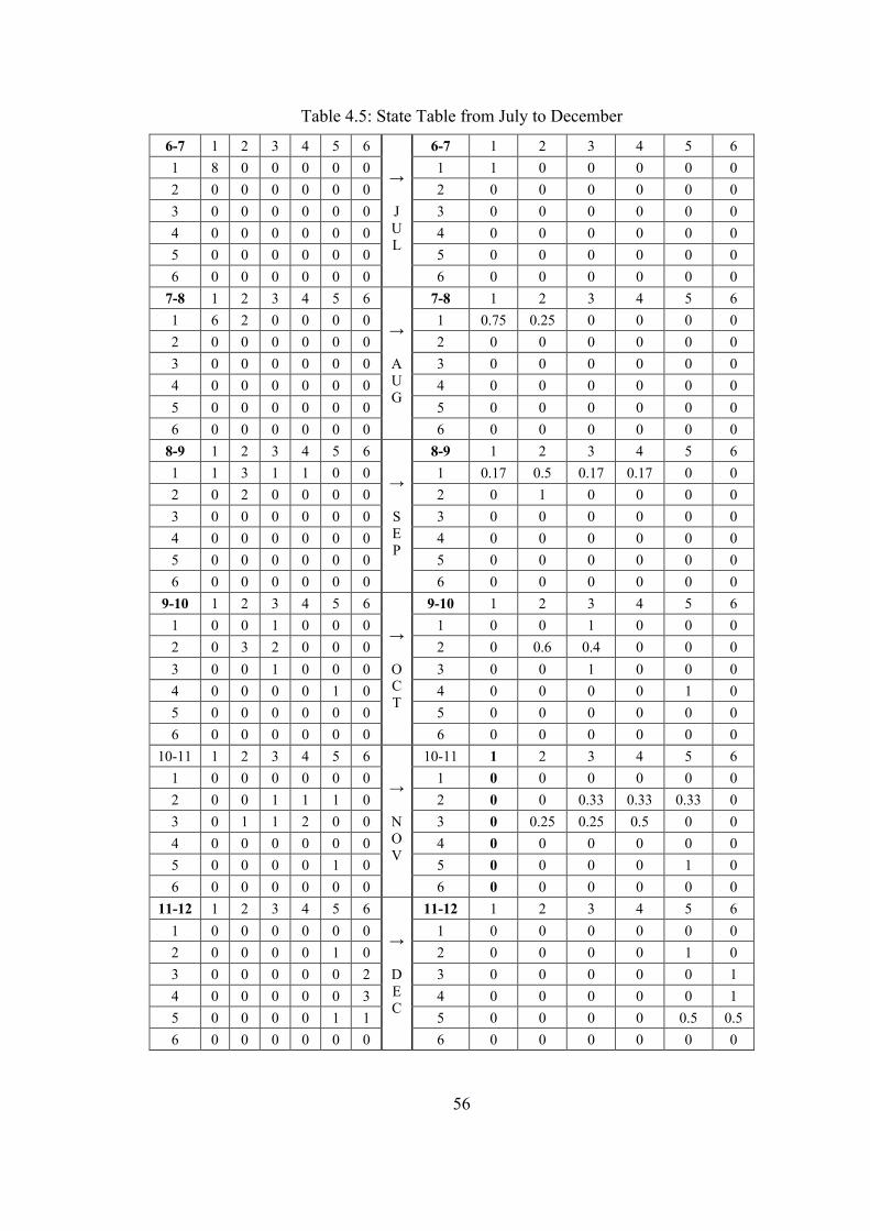
56
Table 4.5: State Table from July to December
6-7 1 2 3 4 5 6
→ J U L
6-7 1 2 3 4 5 6 1 8 0 0 0 0 0 1 1 0 0 0 0 0 2 0 0 0 0 0 0 2 0 0 0 0 0 0 3 0 0 0 0 0 0 3 0 0 0 0 0 0 4 0 0 0 0 0 0 4 0 0 0 0 0 0 5 0 0 0 0 0 0 5 0 0 0 0 0 0 6 0 0 0 0 0 0 6 0 0 0 0 0 0
7-8 1 2 3 4 5 6
→
A U G
7-8 1 2 3 4 5 6 1 6 2 0 0 0 0 1 0.75 0.25 0 0 0 0 2 0 0 0 0 0 0 2 0 0 0 0 0 0 3 0 0 0 0 0 0 3 0 0 0 0 0 0 4 0 0 0 0 0 0 4 0 0 0 0 0 0 5 0 0 0 0 0 0 5 0 0 0 0 0 0 6 0 0 0 0 0 0 6 0 0 0 0 0 0
8-9 1 2 3 4 5 6
→
S E P
8-9 1 2 3 4 5 6 1 1 3 1 1 0 0 1 0.17 0.5 0.17 0.17 0 0 2 0 2 0 0 0 0 2 0 1 0 0 0 0 3 0 0 0 0 0 0 3 0 0 0 0 0 0 4 0 0 0 0 0 0 4 0 0 0 0 0 0 5 0 0 0 0 0 0 5 0 0 0 0 0 0 6 0 0 0 0 0 0 6 0 0 0 0 0 0
9-10 1 2 3 4 5 6
→
O C T
9-10 1 2 3 4 5 6 1 0 0 1 0 0 0 1 0 0 1 0 0 0 2 0 3 2 0 0 0 2 0 0.6 0.4 0 0 0 3 0 0 1 0 0 0 3 0 0 1 0 0 0 4 0 0 0 0 1 0 4 0 0 0 0 1 0 5 0 0 0 0 0 0 5 0 0 0 0 0 0 6 0 0 0 0 0 0 6 0 0 0 0 0 0
10-11 1 2 3 4 5 6
→
N O V
10-11 1 2 3 4 5 6 1 0 0 0 0 0 0 1 0 0 0 0 0 0 2 0 0 1 1 1 0 2 0 0 0.33 0.33 0.33 0 3 0 1 1 2 0 0 3 0 0.25 0.25 0.5 0 0 4 0 0 0 0 0 0 4 0 0 0 0 0 0 5 0 0 0 0 1 0 5 0 0 0 0 1 0 6 0 0 0 0 0 0 6 0 0 0 0 0 0
11-12 1 2 3 4 5 6
→
D E C
11-12 1 2 3 4 5 6 1 0 0 0 0 0 0 1 0 0 0 0 0 0 2 0 0 0 0 1 0 2 0 0 0 0 1 0 3 0 0 0 0 0 2 3 0 0 0 0 0 1 4 0 0 0 0 0 3 4 0 0 0 0 0 1 5 0 0 0 0 1 1 5 0 0 0 0 0.5 0.5 6 0 0 0 0 0 0 6 0 0 0 0 0 0

57
4.4.1.5 Expectations of the Stream Inflow
A value obtained from a random process predicts the forthcoming states. Thus, stream
flow is found as a result of such a process. The process starts by selecting a row,
calculating its result and picking the random state. As a next step, the very row is
selected, its expectations are considered and another state is picked. The process
continues. Mathematically, it can be expressed as follows:
(4.11)
For instance, if row 5 is picked from T-Mat and its expectation is obtained, the values
of the state can be recalled from state tables i.e. Tables 4.3-4.5. The expectation, Exp,
can be calculated as follows: 0.66(1100) + 0.34(900) + 0(700). Therefore, in this
case, the expectation from the above equation will be Exp = 1032. The states along
with their respective conversions and probabilities can be expressed with the help of a
state diagram as shown in Figure 4.1.
Maximum possible hydropower is calculated and distributed among the hydropower
units. On-site, there are five turbines installed with each having the capacity of 290
MW totaling to about 1450 MW. Other particulars of the site are as follows: head
height is 70 meters; monthly discharge capacity is 1600 cubic meter per second
(cumecs); minimum reservoir storage capacity is 800 cumecs and maximum reservoir
storage capacity is 1200 cumecs. The reservoir storage capacity at the end of
December is 1000 cumecs.
4.4.1.6 Reservoir Operation
The operation of reservoir plays a significant role when making a decision about the
discharge of water. Water discharge in hydroelectric depends on the availability of
water and the predicted inflow. In order to ensure continuous availability of water, the
reservoir operation needs to be improved.
)(,....)()( 2211 nn StPStPStPExp +++=

58
4.4.1.7 Reservoir Storage Continuity
• Water storage limitations
Water storage limit describes the maximum and a minimum capacity of a water
storage reservoir. Storage attains the maximum efficiency when the reservoir attains
full capacity. However, it is not possible all the times. Therefore, when the reservoir
operates on half capacity, it is considered acceptable.
(4.12)
• Reservoir constraints
The reservoir continuity equation is given as follows:
(4.13)
• Water discharge and generation limits
Water discharge limits indicate the minimum and maximum water discharge from a
reservoir, and can be expressed as,
(4.14)
In the same manner, there are maximum and minimum power generation figures of a
hydroelectric generating station.
(4.15)
4.4.2 Thermal System Modeling
Hydrothermal Coordination is characterized by cost minimization of thermal power
units. The cost of fuel and emission minimization depends on various factors and is,
therefore, does not remain same all the times. Both such costs are addressed.
Vhjmin <Vhj <Vhj
max
Vhj(t+1) =Vhjt + Et+1 −Qt − S t
Qhjmin <Qhj <Qhj
max
hj
min
P ≤hjtP ≤
hj
max
P , jεhN , t ε T
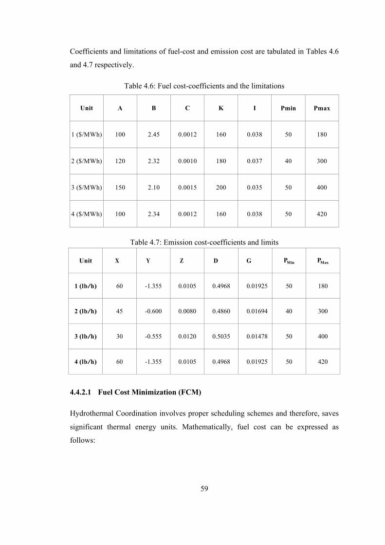
59
Coefficients and limitations of fuel-cost and emission cost are tabulated in Tables 4.6
and 4.7 respectively.
Table 4.6: Fuel cost-coefficients and the limitations
Unit A B C K I Pmin Pmax
1 ($/MWh) 100 2.45 0.0012 160 0.038 50 180
2 ($/MWh) 120 2.32 0.0010 180 0.037 40 300
3 ($/MWh) 150 2.10 0.0015 200 0.035 50 400
4 ($/MWh) 100 2.34 0.0012 160 0.038 50 420
Table 4.7: Emission cost-coefficients and limits
Unit X Y Z D G PMin PMax
1 (lb/h) 60 -1.355 0.0105 0.4968 0.01925 50 180
2 (lb/h) 45 -0.600 0.0080 0.4860 0.01694 40 300
3 (lb/h) 30 -0.555 0.0120 0.5035 0.01478 50 400
4 (lb/h) 60 -1.355 0.0105 0.4968 0.01925 50 420
4.4.2.1 Fuel Cost Minimization (FCM)
Hydrothermal Coordination involves proper scheduling schemes and therefore, saves
significant thermal energy units. Mathematically, fuel cost can be expressed as
follows:

60
(4.16)
The equation (4.16) is only valid for a single steam turbine. In the case of a multi-
steam turbine, the equation changes as follows:
(4.17)
Similar to hydropower plants, thermal generating stations also have a range of limits
for maximum and minimum power generation.
(4.18)
4.4.2.2 Emission Cost Minimization (ECM)
The other vital objective of Hydrothermal Coordination is the minimization of
emission costs. Emissions produced from the burning of fossil fuels negatively impact
the environment. From equation 4.19, it can be inferred that it is essential to minimize
the usage of thermal power in order to reduce GHG emission.
(4.19)
where, total system emission cost and can be equated as:
(4.20)
This equation is valid for a single steam turbine; however, for multiple turbines, the
equation transforms as follows:
minF(PTH ) = xTHi + yTHiPTHit + zTHiPTHit2⎡⎣ ⎤⎦
i=1
NTH
∑t=1
T
∑
F(PTH ) = xTHi + yTHiPTHit + zTHiPTHit2 + uTHi × sin eTHi × PTHi
min − PTHit( ){ }⎡⎣⎢
⎤⎦⎥i=1
NTH
∑t=1
T
∑
THi
min
P ≤THitP ≤
THi
max
P
E(PTHit ) = et PTHit( )i=1
NTH
∑t=1
T
∑
et (PTHit ) = xTHEi + yTHEiPTHit + zTHEiPTHit2

61
(4.21)
4.4.2.3 Combined Fuel and Emission Minimization (CFEM)
So far, the issues relating to fuel and emission have been dealt with gently.
More value can be added by handling the very issues together. This can be
done by adding a ‘penalty factor’.
(4.22)
In Equation 4.22, TOC is the sum of costs. Further, the penalty factor can
be obtained through the following equation:
(4.23)
4.4.2.4 The Objective Function
Objective function with weights and penalty can be written as follows:
(4.24)
here, w1 is the weighted fuel objective and w2 is the weighted emission objective.
The variables P and E have already been derived in equations 4.19 and 4.20
respectively.
The Weighted Objectives Method is a technique used to convert multi objective
function to a simple objective function. This is done by assigning values known as
weights to the variables according to the importance of the variable. The Object
Weight technique assigns weight no greater than 1 and no less than 0 although the
sum of the weights should always be equal to 0. This technique can also be used to
convert more than 10 objectives into a single function and so is used quiet frequently
et = xTHEi + yTHEiPTHit + zTHEiPTHit2 + uTHEi exp(eTHEiPTHit )
minTOC = F(PTHit )+℘E(PTHit )
℘=F(PTHi
max ) / PTHimax
E(PTHimax ) / PTHi
max
minTOC = w1F(PTHit )+ w2λuE(PTHeit )

62
to make simple objective functions. In our problem, we have two conflicting variables
i.e cost minimization and mission rates. To make this multi objective function into a
single function, we have used objective weight technique and thus have been able to
solve a problem simply.
There are some constraints, however, associated with power demand as stated in the
following equation:
(4.25)
The above equation signifies that sum of powers can never exceed or be less than the
demand.
4.5 Proposed Algorithm and Settings
4.5.1 Proposed Algorithm
The main algorithm used in the research work is Particle Swarm Operation (PSO)
technique. It provides accurate results for stochastic values using population
optimization as its primary process. The solution utilizes bio mimicry and learns from
the behavior of birds and fish when they struggle for food in groups. PSO is more
efficient than Genetic Algorithm (GA) in obtaining results, particularly in the case of
random values, which is frequent in power systems. Figure 4.2 depicts the flow-
diagram of PSO algorithm:
Σt=1T PTHi
t + Σt=1T Phj
t + Σt=1T Pwk
t + Σt=1T Psl
t − Pdemandt = 0
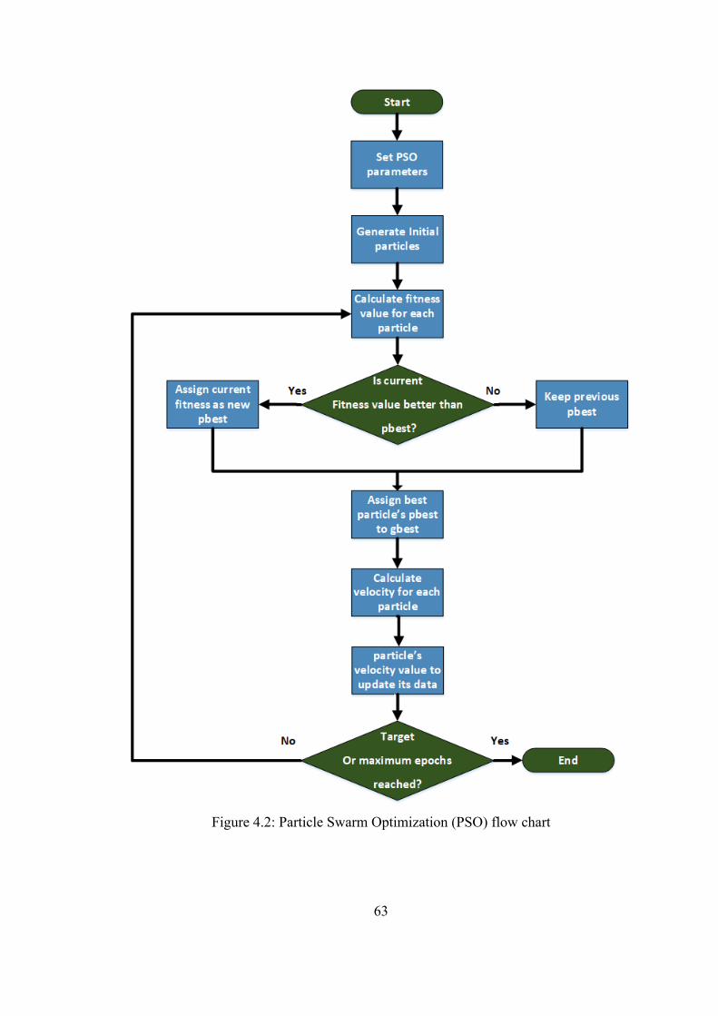
63
Figure 4.2: Particle Swarm Optimization (PSO) flow chart

64
The hydro unit receives the base load and therefore non-thermal load is solved first.
The excess load is then given to the thermal unit. Being stochastic, hydro units are
dealt using the Markov Chains rules. Monte Carlo Iterations are used to balance the
randomness caused by the stochastic nature hydro units.
4.5.2 Particle Swarm Optimization (PSO) Attributes
Dynamic swarm inertia, rather than the static one, was used for the velocity update
process. The Swarm Inertias C1 and C2 were 0.5 and 2.0 respectively in a consecutive
manner. This resulted in enhancement of convergence acceleration and facilitated
more accuracy. By doing so, it is inferred that in order to achieve the best possible
performance, C1 and C2 should be altogether set to the value of 2.50, with assigning
weight to the variables pbest, or local best, and gbest, or global best, in the evolution
process. Using the Particle Swarm Optimization (PSO), a 2-dimensional array of
thermal power and time is formed for each of the power populations. The platform of
MATLAB v 7.12.0 was used for simulation purposes on an Intel (R) Core (TM) i3
workstation having a 4 GB RAM with 1.70 GHz processor.
4.6 Simulation Results
Two hundred (200) PSO generations with 200 iterations of Monte Carlo were
considered. The time period considered is January to December of the following year.
Simulations were run for 11 weights, with each representing a trade-off between Fuel
Cost Minimization (FCM) and Emission Minimization (EM). The eleven weights had
two variables as an array with values stretching from [1,0] to [0,1] and an interval of
0.1 was considered. Each of the individual weights added up 1. The algorithm tries to
minimize the emission as well as fuel cost.
PSO was also consulted to find the convergence of Combined Fuel and Emission
Minimization (CFEM), a parameter which depicts fuel cost and emission as a
combined variable. Figure 4.3 shows the convergence behavior of CFEM.

65
Figure 4.3: Convergence Behavior of Combined Fuel and Emission Minimization
(CFEM)
The algorithm seeks to approach the desired level of minimum cost and reduced
emissions. It must do so while staying within the limit. Initially hydro power is
considered, and then thermal power plants are considered in the next stage. While in
hydropower a water reservoir acts as a power bank. The reservoir can be used all the
year around. Detailed scheduling of all the power plants is shown in Tables 4.8-4.11.

66
Table 4.8: Results of scheduling power plants against the objectives 1,2,3
Month Demand (MW)
PTH1 (MW)
PTH2 (MW)
PTH3 (MW)
PTH4 (MW)
PH1 (MW)
PH2 (MW)
PH3 (MW)
PH4 (MW)
PH5 (MW)
Jan 2035 120 231 258 222 290 290 290 280 35
Feb 1681 180 300 209 293 290 290 76 0 0
Mar 1769 180 296 322 231 290 290 123 0 0
Apr 2053 180 179 233 130 290 290 290 290 130
May 2435 180 300 290 198 290 290 290 290 234
Jun 2695 180 300 323 420 290 290 290 290 274
Jul 2549 180 300 314 250 290 290 290 290 290
Aug 2319 143 213 220 269 290 290 290 290 290
Sep 2017 90 209 156 103 290 290 290 290 286
Oct 1958 175 214 173 50 290 290 290 263 168
Nov 1517 128 181 201 50 290 290 288 75 0
Dec 1362 155 197 242 114 290 290 35 0 0 Objective Weights [F,E] = [0,1] Fuel Cost (M$)=15.295 Emission(Mtons)=25.688
Month Demand (MW)
PTH1 (MW)
PTH2 (MW)
PTH3 (MW)
PTH4 (MW)
PH1 (MW)
PH2 (MW)
PH3 (MW)
PH4 (MW)
PH5 (MW)
Jan 2035 180 202 226 223 290 290 290 280 35
Feb 1681 174 288 324 196 290 290 76 0 0
Mar 1769 180 297 133 419 290 290 123 0 0
Apr 2053 180 145 169 228 290 290 290 290 130
May 2435 146 286 327 210 290 290 290 290 234
Jun 2695 180 300 400 343 290 290 290 290 274
Jul 2549 173 299 268 304 290 290 290 290 290
Aug 2319 180 300 157 208 290 290 290 290 290
Sep 2017 156 117 163 136 290 290 290 290 286
Oct 1958 180 300 145 222 290 290 290 263 168
Nov 1517 150 237 225 50 290 290 288 75 0
Dec 1362 145 249 173 151 290 290 35 0 0
Objective Weights [F,E] = [0.1,0.9] Fuel Cost(M$) =15.253 Emission(Mtons)=25.990
Month Demand (MW)
PTH1 (MW)
PTH2 (MW)
PTH3 (MW)
PTH4 (MW)
PH1 (MW)
PH2 (MW)
PH3 (MW)
PH4 (MW)
PH5 (MW)
Jan 2035 120 231 258 222 290 290 290 280 35
Feb 1681 180 300 209 293 290 290 76 0 0
Mar 1769 180 296 322 231 290 290 123 0 0
Apr 2053 180 179 233 130 290 290 290 290 130
May 2435 180 300 290 198 290 290 290 290 234
Jun 2695 180 300 323 420 290 290 290 290 274
Jul 2549 180 300 314 250 290 290 290 290 290
Aug 2319 143 213 220 269 290 290 290 290 290
Sep 2017 90 209 156 103 290 290 290 290 286
Oct 1958 175 214 173 50 290 290 290 263 168
Nov 1517 128 181 201 50 290 290 288 75 0
Dec 1362 155 197 242 114 290 290 35 0 0 Objective Weights [F,E] = [0.2,0.8] Fuel Cost (M$)=15.124 Emission(Mtons)=25.999

67
Table 4.9: Results of scheduling power plants against the objectives 4,5,6
Month Demand (MW)
PTH1 (MW)
PTH2 (MW)
PTH3 (MW)
PTH4 (MW)
PH1 (MW)
PH2 (MW)
PH3 (MW)
PH4 (MW)
PH5 (MW)
Jan 2035 180 300 144 207 290 290 290 280 35
Feb 1681 180 300 275 227 290 290 76 0 0
Mar 1769 180 300 343 207 290 290 123 0 0
Apr 2053 179 217 201 125 290 290 290 290 130
May 2435 172 295 217 282 290 290 290 290 234
Jun 2695 180 294 328 420 290 290 290 290 274
Jul 2549 180 300 312 253 290 290 290 290 290
Aug 2319 167 258 218 202 290 290 290 290 290
Sep 2017 137 174 202 58 290 290 290 290 286
Oct 1958 180 276 240 145 290 290 290 263 168
Nov 1517 120 247 148 56 290 290 288 75 0
Dec 1362 165 199 215 50 290 290 35 0 0
Objective Weights [F,E]=[0.3,0.7] Fuel Cost(M$)=15.093 Emission(Mtons)=26.032
Month Demand (MW)
PTH1 (MW)
PTH2 (MW)
PTH3 (MW)
PTH4 (MW)
PH1 (MW)
PH2 (MW)
PH3 (MW)
PH4 (MW)
PH5 (MW)
Jan 2035 180 300 212 139 290 290 290 280 35
Feb 1681 180 300 275 226 290 290 76 0 0
Mar 1769 158 274 324 273 290 290 123 0 0
Apr 2053 159 270 152 142 290 290 290 290 130
May 2435 137 270 337 224 290 290 290 290 234
Jun 2695 180 300 323 419 290 290 290 290 274
Jul 2549 180 300 332 233 290 290 290 290 290
Aug 2319 180 229 204 232 290 290 290 290 290
Sep 2017 130 210 182 50 290 290 290 290 286
Oct 1958 180 249 139 278 290 290 290 263 168
Nov 1517 138 108 296 120 290 290 288 75 0
Dec 1362 138 195 230 153 290 290 35 0 0
Objective Weights [F,E]=[0.4,0.6] Fuel Cost(M$)=15.084 Emission(Mtons)=26.166
Month Demand (MW)
PTH1 (MW)
PTH2 (MW)
PTH3 (MW)
PTH4 (MW)
PH1 (MW)
PH2 (MW)
PH3 (MW)
PH4 (MW)
PH5 (MW)
Jan 2035 180 300 229 122 290 290 290 280 35
Feb 1681 180 300 233 269 290 290 76 0 0
Mar 1769 180 300 328 221 290 290 123 0 0
Apr 2053 180 200 126 216 290 290 290 290 130
May 2435 125 286 325 230 290 290 290 290 234
Jun 2695 180 300 322 420 290 290 290 290 274
Jul 2549 180 300 275 290 290 290 290 290 290
Aug 2319 180 214 316 135 290 290 290 290 290
Sep 2017 89 246 187 50 290 290 290 290 286
Oct 1958 180 300 400 223 290 290 290 263 168
Nov 1517 180 108 130 162 290 290 288 75 0
Dec 1362 125 245 301 50 290 290 35 0 0
Objective Weights [F,E]=[0.5,0.5] Fuel Cost(M$)=14.989 Emission(Mtons)=26.262
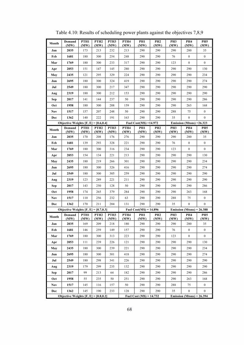
68
Table 4.10: Results of scheduling power plants against the objectives 7,8,9
Month Demand (MW)
PTH1 (MW)
PTH2 (MW)
PTH3 (MW)
PTH4 (MW)
PH1 (MW)
PH2 (MW)
PH3 (MW)
PH4 (MW)
PH5 (MW)
Jan 2035 173 213 232 213 290 290 290 280 35
Feb 1681 180 300 254 248 290 290 76 0 0
Mar 1769 180 300 233 317 290 290 123 0 0
Apr 2053 151 147 145 280 290 290 290 290 130
May 2435 121 295 329 224 290 290 290 290 234
Jun 2695 180 300 324 419 290 290 290 290 274
Jul 2549 180 300 217 347 290 290 290 290 290
Aug 2319 180 300 212 153 290 290 290 290 290
Sep 2017 141 144 237 50 290 290 290 290 286
Oct 1958 180 300 208 159 290 290 290 263 168
Nov 1517 157 207 248 50 290 290 288 75 0
Dec 1362 140 222 191 163 290 290 35 0 0
Objective Weights [F, E] = [0.6,0.4] Fuel Cost(M$) =14.972 Emission (Mtons) =26.323
Month Demand (MW)
PTH1 (MW)
PTH2 (MW)
PTH3 (MW)
PTH4 (MW)
PH1 (MW)
PH2 (MW)
PH3 (MW)
PH4 (MW)
PH5 (MW)
Jan 2035 170 208 176 276 290 290 290 280 35
Feb 1681 139 293 328 221 290 290 76 0 0
Mar 1769 180 300 316 234 290 290 123 0 0
Apr 2053 154 134 221 213 290 290 290 290 130
May 2435 180 219 266 301 290 290 290 290 234
Jun 2695 180 300 326 416 290 290 290 290 274
Jul 2549 180 300 305 259 290 290 290 290 290
Aug 2319 123 289 221 211 290 290 290 290 290
Sep 2017 143 250 128 50 290 290 290 290 286
Oct 1958 174 265 379 284 290 290 290 263 168
Nov 1517 110 256 232 63 290 290 288 75 0
Dec 1362 170 211 204 131 290 290 35 0 0
Objective Weights [F, E] = [0.7,0.3] Fuel Cost(M$) = 14.896 Emission (Mtons) = 26.388
Month Demand (MW)
PTH1 (MW)
PTH2 (MW)
PTH3 (MW)
PTH4 (MW)
PH1 (MW)
PH2 (MW)
PH3 (MW)
PH4 (MW)
PH5 (MW)
Jan 2035 169 209 218 180 290 290 290 280 35
Feb 1681 146 259 149 157 290 290 76 0 0
Mar 1769 180 300 313 223 290 290 123 0 0
Apr 2053 111 239 226 121 290 290 290 290 130
May 2435 180 300 239 221 290 290 290 290 234
Jun 2695 180 300 301 418 290 290 290 290 274
Jul 2549 180 298 341 226 290 290 290 290 290
Aug 2319 179 299 235 132 290 290 290 290 290
Sep 2017 99 213 64 182 290 290 290 290 286
Oct 1958 55 235 50 251 290 290 290 263 168
Nov 1517 145 116 157 50 290 290 288 75 0
Dec 1362 145 190 233 128 290 290 35 0 0 Objective Weights [F, E] = [0.8,0.2] Fuel Cost (M$) = 14.732 Emission (Mtons) = 26.394

69
Table 4.11: Results of scheduling power plants against the objectives 10, 11
In the case of hydropower plants, the primary focus is to control the constraints,
reduce the limitations and ensure smooth functioning of the power plant. The
expected inflow resulting from the Markov Chain is shown in Figure 4.4.
Month Demand (MW)
PTH1 (MW)
PTH2 (MW)
PTH3 (MW)
PTH4 (MW)
PH1 (MW)
PH2 (MW)
PH3 (MW)
PH4 (MW)
PH5 (MW)
Jan 2035 158 203 192 184 290 290 290 280 35
Feb 1681 159 290 131 224 290 290 76 0 0
Mar 1769 180 300 329 214 290 290 123 0 0
Apr 2053 145 282 153 130 290 290 290 290 130
May 2435 177 299 225 253 290 290 290 290 234
Jun 2695 180 268 345 416 290 290 290 290 274
Jul 2549 180 300 336 228 290 290 290 290 290
Aug 2319 180 242 237 186 290 290 290 290 290
Sep 2017 118 166 142 132 290 290 290 290 286
Oct 1958 180 300 137 299 290 290 290 263 168
Nov 1517 76 266 119 192 290 290 288 75 0
Dec 1362 179 237 145 149 290 290 35 0 0
Objective Weights [F, E] = [0.9,0.1] Fuel Cost (M$) = 14.692 Emission (Mtons) = 26.449
Month Demand (MW)
PTH1 (MW)
PTH2 (MW)
PTH3 (MW)
PTH4 (MW)
PH1 (MW)
PH2 (MW)
PH3 (MW)
PH4 (MW)
PH5 (MW)
Jan 2035 122 137 349 129 290 290 290 280 35
Feb 1681 53 228 216 216 290 290 76 0 0
Mar 1769 180 300 239 297 290 290 123 0 0
Apr 2053 127 223 140 208 290 290 290 290 130
May 2435 180 300 235 225 290 290 290 290 234
Jun 2695 180 300 400 319 290 290 290 290 274
Jul 2549 180 300 282 282 290 290 290 290 290
Aug 2319 180 197 305 163 290 290 290 290 290
Sep 2017 159 127 222 50 290 290 290 290 286
Oct 1958 131 134 187 140 290 290 290 263 168
Nov 1517 156 138 131 127 290 290 288 75 0
Dec 1362 180 209 140 181 290 290 35 0 0 Objective Weights [F, E] = [1,0] Fuel Cost(M$) = 15.237 Emission (Mtons) = 26.501

70
Figure 4.4: Expected Water Inflow and Discharge
The annual monthly reservoir water inflow is shown in Figure 4.5. water inflow is
more in summer season due to the ice melting on the mountain of north.
Figure 4.5: Reservoir storage profile throughout the year

71
Figure 4.6 depicts the monthly electrical power generated from Thermal and Hydro,
power plant. Load demand is more during the summer season as compared to winter,
due to the air-conditioning requirement in Pakistan.
Figure 4.6: Load demand vs generation by power plants
Figure 4.7: Cost of Fuel with respect to Objectives
13.6
13.8
14
14.2
14.4
14.6
14.8
15
15.2
15.4
[0,1] [0.1,0.9] [0.2,0.8] [0.3,0.7] [0.4,0.6] [0.5,0.5] [0.6,0.4] [0.7,0.3] [0.8,0.2] [0.9,0.1] [1,0]
Cos
t in
M$
Objective Weightage [F,E]
Cost

72
Figure 4.7 represents the cost of fuel with respect to its objective weightage. It can be
observed from the graph that as the variable F, or weight of fuel cost, increases, the
fuel cost decreases. The case is vice versa for coordinate E, or objective weightage of
the GHG emissions.
Figure 4.8: Emission with respect to objectives
Figure 4.8 shows emissions with respect to the objective function. It can be observed
from the graph that as the variable F, or objective weightage of fuel-cost, increases,
emissions increase. And, as objective weightage of emissions, or E, decreases, the
proportion of emissions increase.
Pareto distribution of emission versus the cost of fuel is shown in Figure 4.9. It is
observed that the cost of fuel and emission are conflicting objectives. Here, the
algorithm tries to minimize both the cost of fuel and the GHG emissions. However, it
does so to a certain limit. As the cost decreases, the emission increases. Therefore,
practically, most of the cheaper thermal power plants are often characterized by
increased levels of air pollution.
25.2
25.4
25.6
25.8
26
26.2
26.4
26.6
[0,1] [0.1,0.9] [0.2,0.8] [0.3,0.7] [0.4,0.6] [0.5,0.5] [0.6,0.4] [0.7,0.3] [0.8,0.2] [0.9,0.1] [1,0]
Em
issi
on in
Mlb
s
Objective Weightage [F,E]
Emission

73
Figure 4.9: Pareto Function of fuel cost and the resulting emissions
4.7 Chapter Conclusion
The major objective of hydrothermal power systems is to meet energy requirements as
well as to protect the environment. In this chapter, Markov Chain is used to predict
the water inflow of Ghazi Barotha Hydropower Plant. Particle Swarm Optimization
(PSO) is implemented to handle the disparate problems by assigning unique
weightage to each of the objectives. This has, in turn, led us to come forth with
results, which depict the conflicting nature of emission and fuel.
14.0
14.2
14.4
14.6
14.8
15.0
15.2
15.4
25.6 25.7 25.8 25.9 26.0 26.1 26.2 26.3 26.4 26.5 26.6
Cost
in M
illio
n Do
llars
(M$)
Emssion in Million Pounds (Mlbs)

74
5 Short-Term Hydrothermal Coordination (STHTC)
75
5.1 Chapter Summary
The chapter addresses Short-term Hydrothermal Coordination (STHTC), which deals
with durations lasting from 1 hour to 1 week. A viable global optimizer, based on
Chaotic Differential Evolution (CDE), is combined with Sequential Quadratic
Programming (SQP), an efficient local search technique. This results in an efficient
Short-term Hydrothermal Coordination (STHTC) scheme. A multi-objective
optimization framework is established for minimizing the total cost of thermal
generators with valve-point loading effects. The proposed model is implemented on
various systems comprising of hydro generating and thermal units. Monte Carlo
simulations are used to analyze and validate the reliability, stability and effectiveness
of the proposed framework.
5.2 Related Work and Case-studies
In the power sector, optimum coordination of demand and generation substantially
impacts the budget. Most of the research endeavors are focused on minimization of
cost and power losses [120, 121]. To a larger extent, electrical power systems of the
day comprise of thermal and hydropower plants connected via transmission networks
[122]. One of the foremost objectives in power systems is to meet power demand
economically by utilizing the optimal mix of generation technologies. Huge savings in
fuel cost are achieved if the available hydro-electric resources are utilized in a manner
ensuring minimal wastage of water [123]. One of the major objectives of
Hydrothermal Coordination is cost minimization of the power generation systems.
This is achieved by adopting a multi-pronged approach keeping in view multiple
factors such as transmission losses, available resources, fuel cost, load variations and
valve point loading etc.
Derivative-free methods have the ability to converge and are less likely to get stuck in
local minima when attempting to seek a global solution. Besides, their computational
complexity is also not an issue, most of the times [124-126].
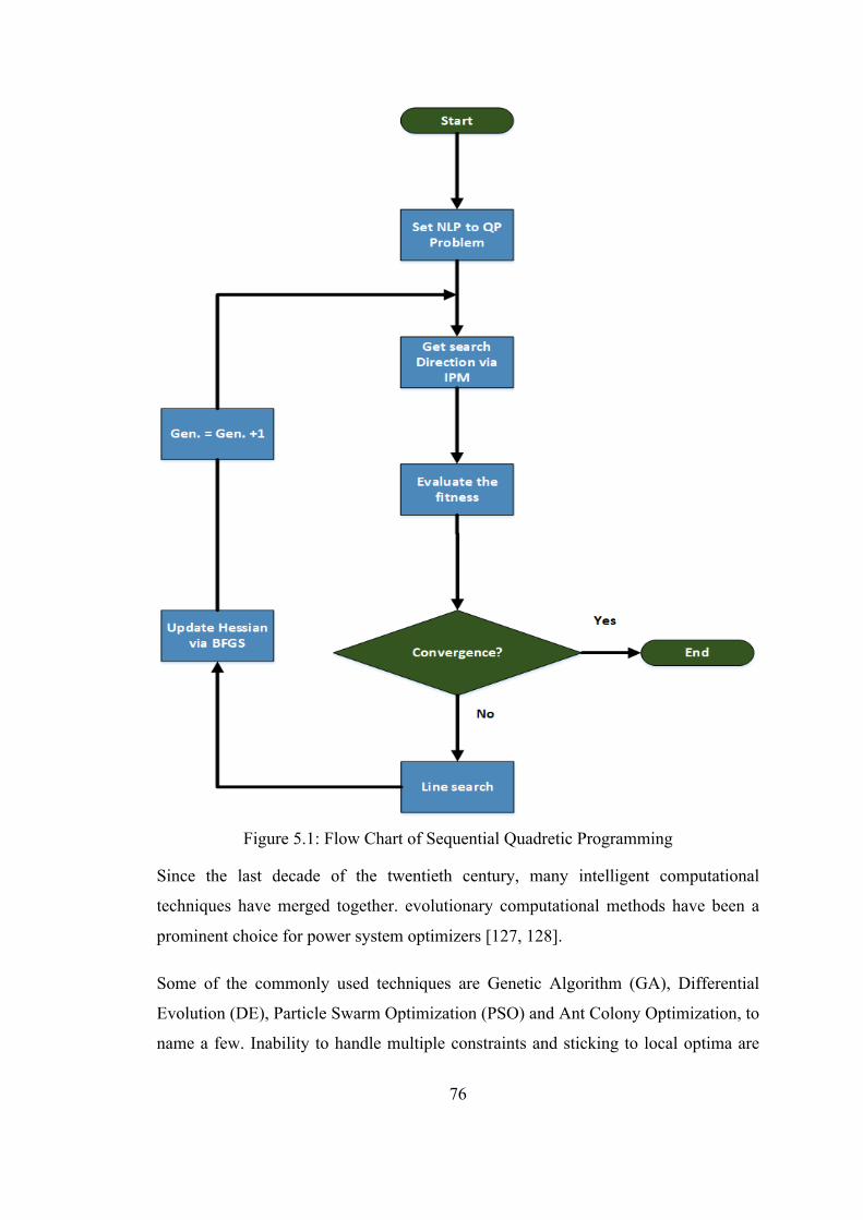
76
Figure 5.1: Flow Chart of Sequential Quadretic Programming
Since the last decade of the twentieth century, many intelligent computational
techniques have merged together. evolutionary computational methods have been a
prominent choice for power system optimizers [127, 128].
Some of the commonly used techniques are Genetic Algorithm (GA), Differential
Evolution (DE), Particle Swarm Optimization (PSO) and Ant Colony Optimization, to
name a few. Inability to handle multiple constraints and sticking to local optima are
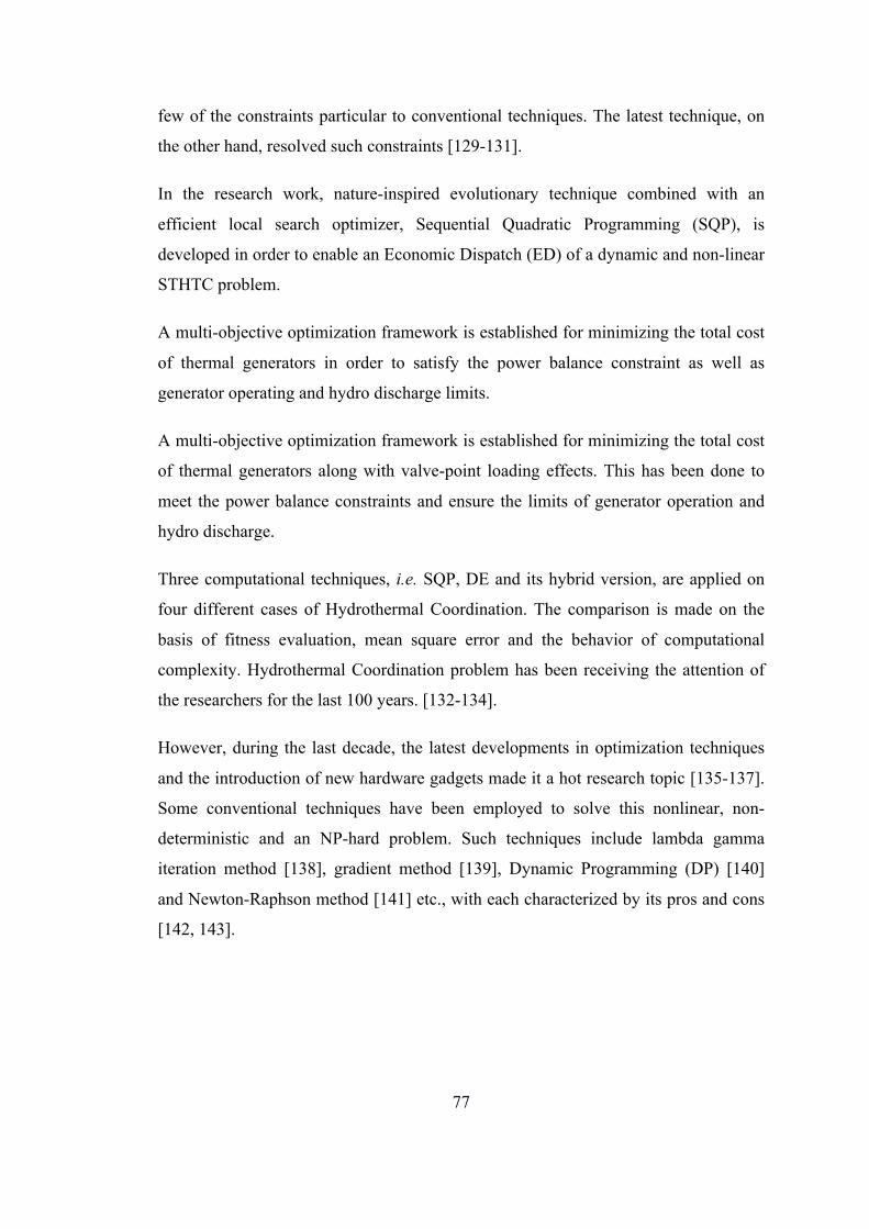
77
few of the constraints particular to conventional techniques. The latest technique, on
the other hand, resolved such constraints [129-131].
In the research work, nature-inspired evolutionary technique combined with an
efficient local search optimizer, Sequential Quadratic Programming (SQP), is
developed in order to enable an Economic Dispatch (ED) of a dynamic and non-linear
STHTC problem.
A multi-objective optimization framework is established for minimizing the total cost
of thermal generators in order to satisfy the power balance constraint as well as
generator operating and hydro discharge limits.
A multi-objective optimization framework is established for minimizing the total cost
of thermal generators along with valve-point loading effects. This has been done to
meet the power balance constraints and ensure the limits of generator operation and
hydro discharge.
Three computational techniques, i.e. SQP, DE and its hybrid version, are applied on
four different cases of Hydrothermal Coordination. The comparison is made on the
basis of fitness evaluation, mean square error and the behavior of computational
complexity. Hydrothermal Coordination problem has been receiving the attention of
the researchers for the last 100 years. [132-134].
However, during the last decade, the latest developments in optimization techniques
and the introduction of new hardware gadgets made it a hot research topic [135-137].
Some conventional techniques have been employed to solve this nonlinear, non-
deterministic and an NP-hard problem. Such techniques include lambda gamma
iteration method [138], gradient method [139], Dynamic Programming (DP) [140]
and Newton-Raphson method [141] etc., with each characterized by its pros and cons
[142, 143].
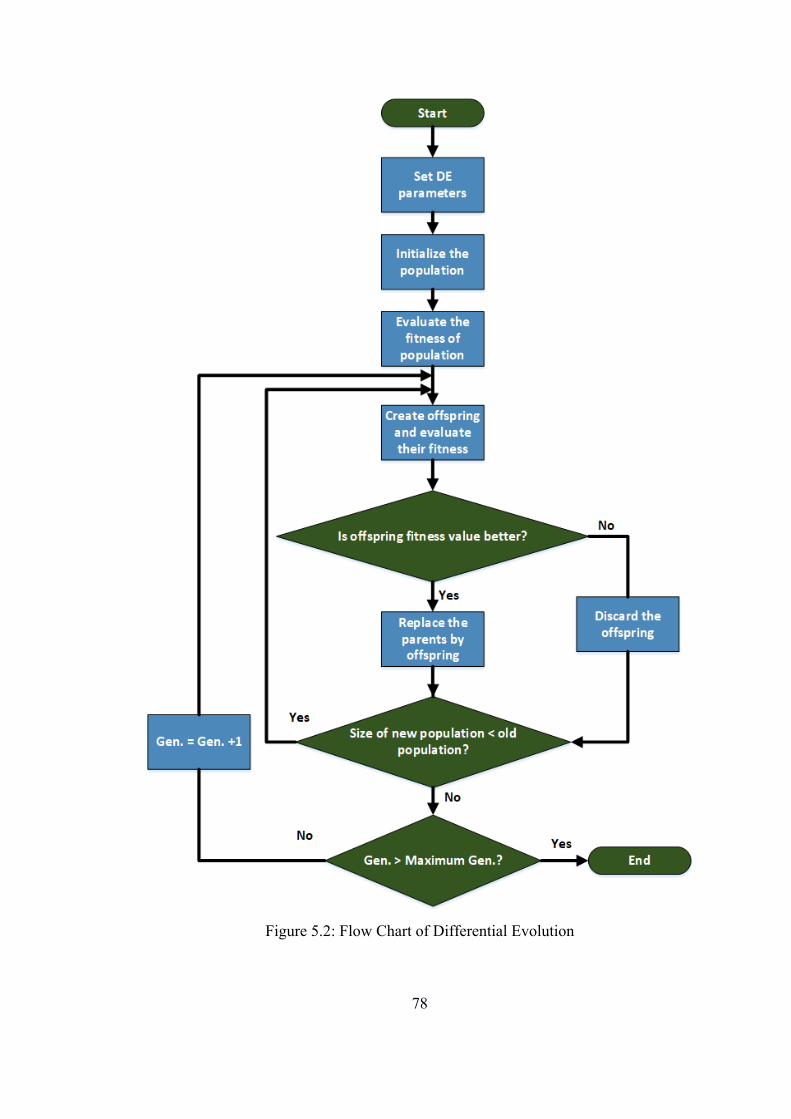
78
Figure 5.2: Flow Chart of Differential Evolution
79
Although conventional techniques can offer a reasonable and timely solution, they are
unable to handle more constraints and are prone to stick in the issue of local minima.
The schemes, like priority list method, a class of weighted procedures, and forward
Dynamic Programming (DP) approach, received attention from researchers as such
schemes handled the problem of Unit Commitment (UC) in an elegant manner. [144,
145] Despite, the probability of getting stuck in the local minimum persists. Almost
similar problems have been observed in the Lagrange relaxation method and the class
method based on Karush Kuhn Tucker equations [143, 146].
In this chapter, case studies consulted are taken from [120, 147-150]; section 4
contains the discussion; and conclusion is presented in the end.
5.3 Problem Formulation
One of the chief aims of Hydrothermal Coordination is to minimize the fuel cost and
address the power demand constraints. The objective function for Hydrothermal
Coordination is given in Equation 4.17.
5.3.1 System Constraints
In each interval of the scheduled time, the output power produced by hydroelectric
and thermal power plants must balance the expected power demand and transmission
line losses.
(5.1)
Hydroelectric power production depends on water discharge and water head; both of
them are directly related to the storage volume of the reservoir.
(5.2)
Power losses due to transmission are given as in Equation 5.3.
PTHit + Phjtj=1
Nh
∑ = Pdt + Plt , t ∈Ti=1
NTH
∑
Phjt = C1 jVhjt2 +C2 jQhjt
2 +C3 jVhjtQhjt +C4 jVhjt +C5 jVhjt +C6 j
80
(5.3)
The above-mentioned equation indicates that each thermal generation unit has certain
upper and lower generation limits. The output power extracted from a unit should be
in the given generation range. Thermal power plants also have lower and upper limits
of generation given in Equations 4.18. Similarly, there are limits to hydroelectric
power as shown in Equation 4.15.
The power produced from a thermal unit ‘i’ during a particular interval should not
exceed the power generated in the previous interval by a certain defined amount. In
the same way, the power produced should not be less than the power generated in the
previous interval by a certain limit.
Mathematically, it can be represented in terms of Up Ramp (UR) and Down Ramp
(DR) as shown in Equations 5.4 and 5.5 respectively.
(5.4)
(5.5)
There are several challenges which hamper the smooth operation of a hydropower
plant. These include maintaining a balanced quantity of water, lowering the power
plant limitations and ensuring multipurpose storage etc. Stated earlier, the equations
4.12 and 4.14 are used to express the storage volume and discharge rate of reservoir
respectively.
5.4 Chaotic Differential Evolution (CDE) and Quadratic
Programming (QP)
Differential Evolution (DE) algorithm is a robust meta-heuristic method for function
minimization/maximization. It was proposed by Ken and Storm in 1997 [151]. DE is
Plt = PitBijPjtj=1
NTH +Nh
∑i=1
NTH +Nh
∑ + Boii=1
NTH +Nh
∑ Pit + Boo
PTHit − PTHi(t−1) ≤URi
PTHi(t−1) − PTHit ≤ DRi

81
a population-based stochastic algorithm with few parameters; but, because it is not a
gradient-based method, it offers an excellent solution to the non-smooth, multimodal
and non-convex problems [152] [153]. As compared to other Evolutionary algorithms,
DE is less stochastic but more greedy and uses simple arithmetic operators [154].
DE differs from the Genetic Algorithm (GA) in that it uses perturbing vectors. The
perturbing vectors cause diversity in each of the sample space. Besides, the
amplification factor in DE searches for the candidate solution thoroughly on the
solution surface [155].
DE finds its use in various research areas such as electrical power simulations, optical
systems optimization, radio network designs and water pumping systems optimization
[156]. DE has some drawbacks. To overcome some of the common drawbacks of DE,
chaotic theory is made into use.
DE should be made chaotic enough to assure diversification. This enabled the handle
to move through the whole search space. As a result, the probability of being caught
in local optima is reduced significantly and the parameter control strategy is further
enhanced Flow chart of the chaotic DE is shown in Fig. 5.3.
More precisely, to create diversity in the search space, the behavior of a chaotic
system is encapsulated in the differential evolutionary algorithm using Gaussian
randomness. As a result, the algorithm will perform the search operation thoroughly.
The vector representation and factor of DE algorithm is also coupled with the chaotic
variable. This guarantees the parallelism in n-dimensions and improves the
computational searching of the proposed scheme.
SQP is an iterative method that falls under the class of barrier methods and it can be
used efficiently for nonlinear optimization of complex systems having linear and/or
non-linear constraints. Flow chart of SQP is shown in Fig. 5.1.

82
Figure 5.3: Flow Chart of Chaotic Differential Evolution
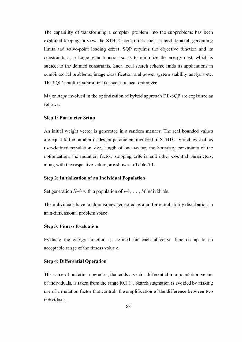
83
The capability of transforming a complex problem into the subproblems has been
exploited keeping in view the STHTC constraints such as load demand, generating
limits and valve-point loading effect. SQP requires the objective function and its
constraints as a Lagrangian function so as to minimize the energy cost, which is
subject to the defined constraints. Such local search scheme finds its applications in
combinatorial problems, image classification and power system stability analysis etc.
The SQP’s built-in subroutine is used as a local optimizer.
Major steps involved in the optimization of hybrid approach DE-SQP are explained as
follows:
Step 1: Parameter Setup
An initial weight vector is generated in a random manner. The real bounded values
are equal to the number of design parameters involved in STHTC. Variables such as
user-defined population size, length of one vector, the boundary constraints of the
optimization, the mutation factor, stopping criteria and other essential parameters,
along with the respective values, are shown in Table 5.1.
Step 2: Initialization of an Individual Population
Set generation N=0 with a population of i=1, …., M individuals.
The individuals have random values generated as a uniform probability distribution in
an n-dimensional problem space.
Step 3: Fitness Evaluation
Evaluate the energy function as defined for each objective function up to an
acceptable range of the fitness value ε.
Step 4: Differential Operation
The value of mutation operation, that adds a vector differential to a population vector
of individuals, is taken from the range [0.1,1]. Search stagnation is avoided by making
use of a mutation factor that controls the amplification of the difference between two
individuals.

84
Step 5: Recombination Operation
Recombination is employed to generate a trial vector. It is done by replacing certain
parameters of the target vector with the corresponding parameters of a randomly
generated donor vector. The recombination rate is taken in a logarithmic manner in
order to obtain mature exploitation of the search space.
Step 6: Selection Operator
The procedure of producing better off-springs is obtained in this step. Here, the
criterion of comparing the fitness of the current individual acts as stability to enter the
next generation. Similarly, the fitness cost of each trial vector is compared with that of
its parent target vector.
If the cost of the target vector is lower than that of the trial vector, the target is
allowed to advance into the next generation. Else, the target vector is replaced by the
trial vector in the next generation.
Step 7: Stopping Criteria for Chaotic Differential Evolution (CDE)
Set the generation number for N=N+1 and proceed to step 3 until a stopping criterion
is fulfilled. The criterion is problem dependent based on the following conditions:
i) A maximum number of generations is achieved. ii) Fitness value ε less than 10-12 is achieved. iii) Function tolerance is lower than a certain pre-defined criteria.
Step 8: Hybrid with SQP
One of the best elements obtained from Chaotic DE is passed as a starting point to the
SQP algorithm. This fine-tunes the unknown adaptive parameters of the STHTC
problem. The flow chart DE-SQP is shown in Fig. 5.4.

85
Figure 5.4: Flow Chart of Chaotic Differential Evolution (CDE) Hybridized with SQP

86
The detailed pseudo-code of the proposed scheme is given as follows:
Input: Psize, STHTCsize, β, Crate, ζ
Output: Rbest= [PTHit Phj]
Population ←initilize population(Psize, STHTCsize)
Evaluatepopulation(Pop)
Rbest ← getbestcandiadte(Pop)
While(stopingcriteria() not met)
newpop←Ø
for popiϵ Pop
Ri←newsample(popi,population, STHTCsize, β,Crate,ζ)
If (fval (Ri)≤ fval (popi))
newpapulation← Ri
Else
newpapulation← popi
End
End
Pop ←newpopulation
Evaluatepopulation(Pop)
Rbest←getbestcandidate(Pop)
End
Return(Rbest)

87
5.5 Simulation and Results
Four scenario-based hydrothermal test systems have been investigated and the
simulation results are presented. The simulation results are based on various
performance criteria such as dollar cost, energy fitness function, the absolute error of
load and generation, and the temporal computational complexity. The level and
percentage of the convergence for chaotic DE, SQP and hybrid approach are also
computed for a large number of iterations. The algorithms are implemented by using
MATLAB version 7.12.0 (R 2011a) on the Intel(R) Core (TM) i3-4010U CPU @
1.70 GHz machine with 4GB RAM.
Table 5.1: Parameter Values/Settings for Chaotic Differential Evolution and
Sequential Quadratic Programming
Chaotic Differential Evolution Sequential Quadratic Programming
Parameters Values/ Settings Parameters Values/ Settings
Generations 500 Start point The random or best
result of CDE
Population size 360 No of variables Generation Unit
Dependent
Population Range [-1 1] Iterations 1000
Function Tolerance 10-30 Max. Function
Evaluations 50000
Stall Generation Limit
200 Function Tolerance 0
Nonlinear Constraints tolerance
10-30 Nonlinear
Constraints tolerance
0
Fitness Limit 10-35 Derivative approach
Finite forward difference
X-Tolerance 10-18 X-Tolerance 10-18
Bounds As given in
thermal units Bounds
As given in thermal units
Others Default Others Default
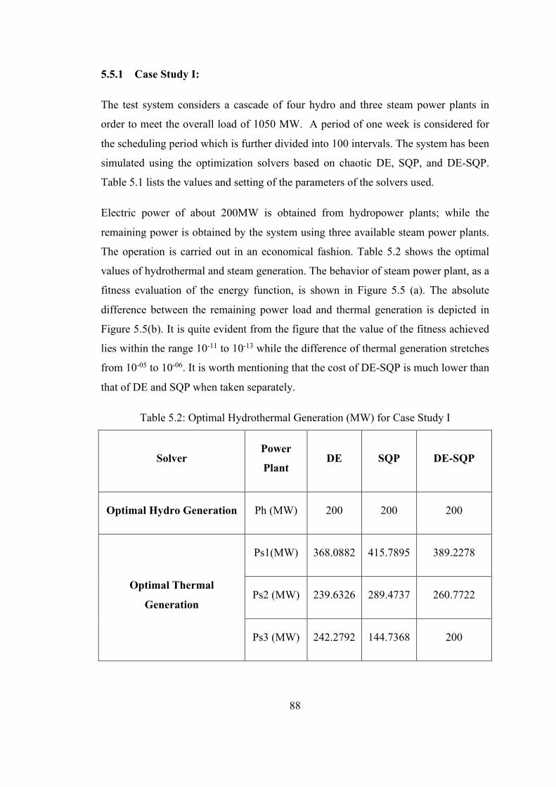
88
5.5.1 Case Study I:
The test system considers a cascade of four hydro and three steam power plants in
order to meet the overall load of 1050 MW. A period of one week is considered for
the scheduling period which is further divided into 100 intervals. The system has been
simulated using the optimization solvers based on chaotic DE, SQP, and DE-SQP.
Table 5.1 lists the values and setting of the parameters of the solvers used.
Electric power of about 200MW is obtained from hydropower plants; while the
remaining power is obtained by the system using three available steam power plants.
The operation is carried out in an economical fashion. Table 5.2 shows the optimal
values of hydrothermal and steam generation. The behavior of steam power plant, as a
fitness evaluation of the energy function, is shown in Figure 5.5 (a). The absolute
difference between the remaining power load and thermal generation is depicted in
Figure 5.5(b). It is quite evident from the figure that the value of the fitness achieved
lies within the range 10-11 to 10-13 while the difference of thermal generation stretches
from 10-05 to 10-06. It is worth mentioning that the cost of DE-SQP is much lower than
that of DE and SQP when taken separately.
Table 5.2: Optimal Hydrothermal Generation (MW) for Case Study I
Solver Power
Plant DE SQP DE-SQP
Optimal Hydro Generation Ph (MW) 200 200 200
Optimal Thermal
Generation
Ps1(MW) 368.0882 415.7895 389.2278
Ps2 (MW) 239.6326 289.4737 260.7722
Ps3 (MW) 242.2792 144.7368 200

89
(a)
(b)
Figure 5.5: (a) Behavior of the fitness function evaluation; (b) Absolute error of thermal generation for 100 intervals
Table 5.3: Optimal Hydrothermal Generation (MW) for Case Study II
t(h) ph1
(MW)
ph2
(MW)
ph3
(MW)
ph4
(MW)
Pgt
(MW)
Cost
(103 $) 1 21.60 17.47 43.98 44.20 62.77 3597.68 2 28.08 16.24 41.06 43.72 40.90 2245.36 3 31.02 16.18 39.88 47.46 35.46 1983.18 4 21.01 20.41 38.83 42.13 67.63 3962.82 5 37.03 15.93 38.41 53.76 44.87 2455.54 6 34.18 19.38 32.50 49.44 74.51 4521.18 7 33.24 22.92 35.78 44.62 93.43 6298.71 8 48.17 22.43 30.89 52.03 96.50 6620.86 9 60.70 22.85 35.02 58.83 92.60 6213.33
10 56.53 31.32 31.49 53.28 137.36 11807.85 11 65.33 32.21 35.42 63.37 153.67 14343.23 12 55.45 29.30 34.85 59.14 131.26 10927.52 13 50.80 34.22 39.34 60.99 164.65 16201.02 14 62.13 29.34 41.75 71.71 145.07 12973.61 15 59.60 25.41 44.59 72.71 107.69 7875.86 16 46.61 26.77 42.18 66.97 107.47 7849.89 17 44.97 24.27 43.11 68.84 88.84 5834.52 18 41.09 22.26 43.60 69.43 73.62 4446.19 19 34.13 20.96 43.50 68.37 63.03 3616.75 20 38.38 15.51 46.19 75.20 34.71 1949.64 21 38.54 17.39 44.08 74.63 35.36 1978.84 22 26.41 23.67 42.22 64.35 53.35 2956.72 23 39.58 9.71 42.27 72.97 25.48 1579.30 24 28.02 13.00 40.61 64.28 44.09 2413.00
Total Cost = 144652.61

90
5.5.2 Case Study II
This test system comprises of four hydropower plants and equivalent thermal
generation plant to meet the load requirement. The entire scheduling period is one day
which is further divided into 24 equal intervals. The optimal values of the
hydrothermal generation and steam generation are presented in Table 5.3. The
behavior of the power plant is shown in Figure 5.6 (a) as a fitness evaluation of the
energy function. Figure 5.6(b) shows the absolute difference between the required and
generated power.
(a)
(b)
Figure 5.6: Behavior of the fitness function value (a) and absolute error of thermal generation for 100 intervals in (b)
It is very clear from the figure that the value of the fitness achieved lie in the range
from 10-12 to 10-15 while the difference of thermal generation ranges from 10-06 to 10-
07. It can be observed that the cost for DE-SQP is much lesser when compared to each
of the DE and SQP.
Table 5.4: Results of generation hydro and thermal generations Min Max mean Std. CB DE 153.59 161.43 156.112 0.689 46.7 SQP 170.129 181.62 175.9 1.643 87.5 DE-SQP 144.652 162.89 155.654 0.697 97.38
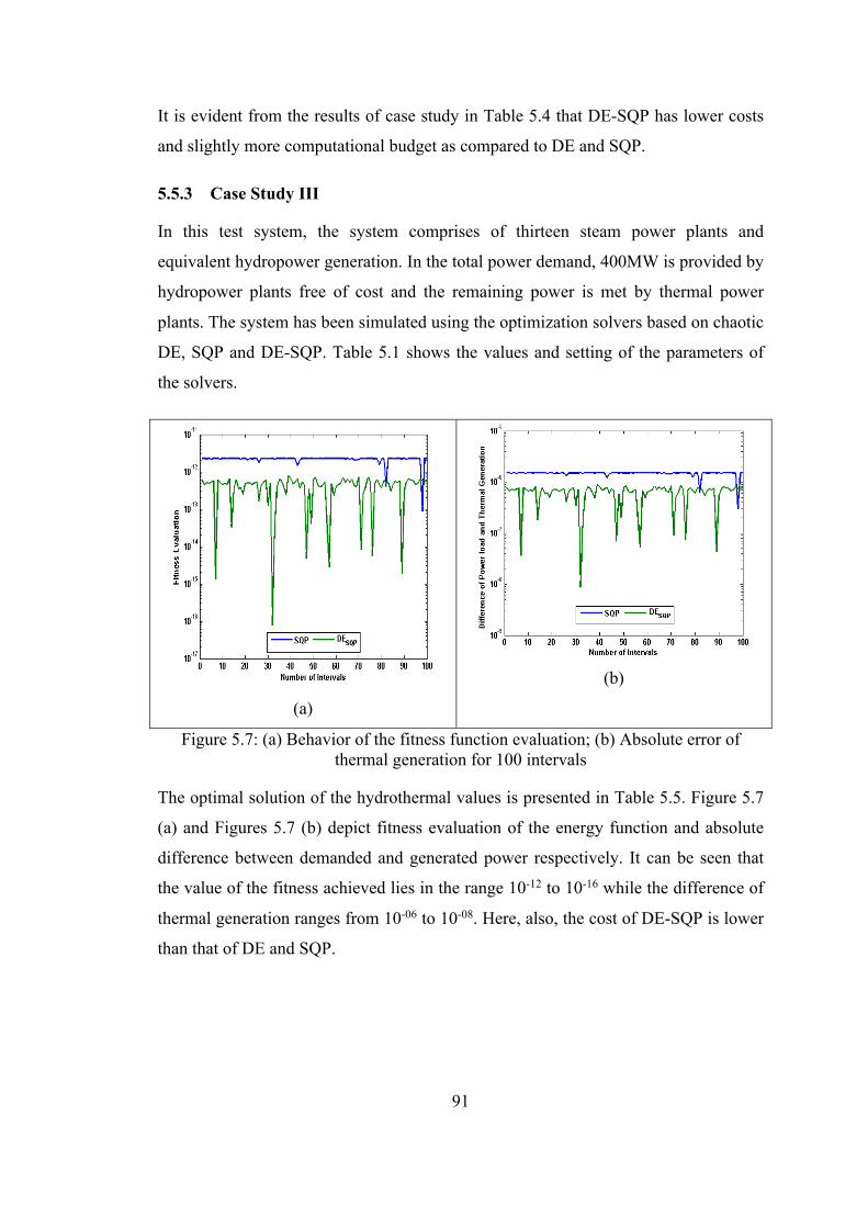
91
It is evident from the results of case study in Table 5.4 that DE-SQP has lower costs
and slightly more computational budget as compared to DE and SQP.
5.5.3 Case Study III
In this test system, the system comprises of thirteen steam power plants and
equivalent hydropower generation. In the total power demand, 400MW is provided by
hydropower plants free of cost and the remaining power is met by thermal power
plants. The system has been simulated using the optimization solvers based on chaotic
DE, SQP and DE-SQP. Table 5.1 shows the values and setting of the parameters of
the solvers.
(a)
(b)
Figure 5.7: (a) Behavior of the fitness function evaluation; (b) Absolute error of thermal generation for 100 intervals
The optimal solution of the hydrothermal values is presented in Table 5.5. Figure 5.7
(a) and Figures 5.7 (b) depict fitness evaluation of the energy function and absolute
difference between demanded and generated power respectively. It can be seen that
the value of the fitness achieved lies in the range 10-12 to 10-16 while the difference of
thermal generation ranges from 10-06 to 10-08. Here, also, the cost of DE-SQP is lower
than that of DE and SQP.
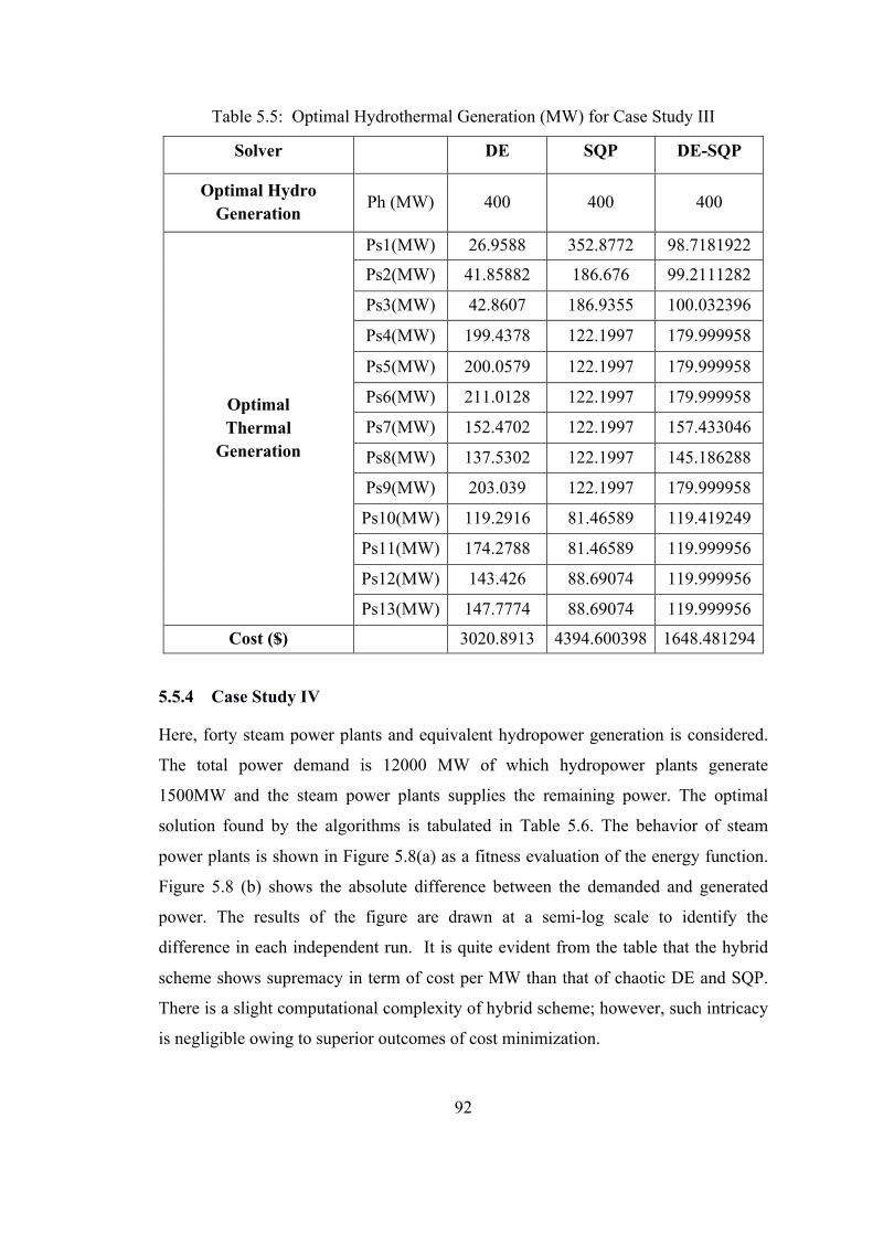
92
Table 5.5: Optimal Hydrothermal Generation (MW) for Case Study III
Solver DE SQP DE-SQP
Optimal Hydro Generation Ph (MW) 400 400 400
Optimal Thermal
Generation
Ps1(MW) 26.9588 352.8772 98.7181922
Ps2(MW) 41.85882 186.676 99.2111282
Ps3(MW) 42.8607 186.9355 100.032396
Ps4(MW) 199.4378 122.1997 179.999958
Ps5(MW) 200.0579 122.1997 179.999958
Ps6(MW) 211.0128 122.1997 179.999958
Ps7(MW) 152.4702 122.1997 157.433046
Ps8(MW) 137.5302 122.1997 145.186288
Ps9(MW) 203.039 122.1997 179.999958
Ps10(MW) 119.2916 81.46589 119.419249
Ps11(MW) 174.2788 81.46589 119.999956
Ps12(MW) 143.426 88.69074 119.999956
Ps13(MW) 147.7774 88.69074 119.999956
Cost ($) 3020.8913 4394.600398 1648.481294
5.5.4 Case Study IV
Here, forty steam power plants and equivalent hydropower generation is considered.
The total power demand is 12000 MW of which hydropower plants generate
1500MW and the steam power plants supplies the remaining power. The optimal
solution found by the algorithms is tabulated in Table 5.6. The behavior of steam
power plants is shown in Figure 5.8(a) as a fitness evaluation of the energy function.
Figure 5.8 (b) shows the absolute difference between the demanded and generated
power. The results of the figure are drawn at a semi-log scale to identify the
difference in each independent run. It is quite evident from the table that the hybrid
scheme shows supremacy in term of cost per MW than that of chaotic DE and SQP.
There is a slight computational complexity of hybrid scheme; however, such intricacy
is negligible owing to superior outcomes of cost minimization.
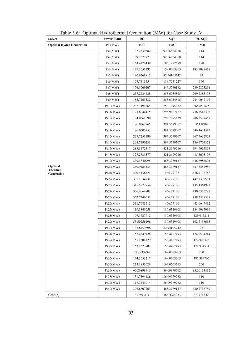
93
Table 5.6: Optimal Hydrothermal Generation (MW) for Case Study IV Solver Power Plant DE SQP DE-SQP
Optimal Hydro Generation Ph (MW) 1500 1500 1500
Optimal Thermal Generation
Ps1(MW) 132.2539582 92.06804958 114
Ps2(MW) 139.2677773 92.06804958 114
Ps3(MW) 163.4171438 103.1292689 120
Ps4(MW) 177.1651195 159.0703263 183.7098418
Ps5(MW) 140.9268812 82.94105742 97
Ps6(MW) 167.7413554 119.7551227 140
Ps7(MW) 176.1009267 246.5760182 239.2873291
Ps8(MW) 237.2224228 253.6054895 269.2385135
Ps9(MW) 185.7263532 253.6054895 244.0047197
Ps10(MW) 232.3491264 252.1995952 266.850625
Ps11(MW) 173.6844415 295.9887427 276.3542302
Ps12(MW) 194.0661898 296.7075639 286.8509457
Ps13(MW) 196.0262765 394.5579307 351.0504
Ps14(MW) 186.0605753 394.5579307 346.1671317
Ps15(MW) 229.7251196 394.5579307 367.5632823
Ps16(MW) 268.7190231 394.5579307 386.6704321
Ps17(MW) 285.1172317 421.2699216 394.7055833
Ps18(MW) 327.2881577 421.2699216 415.3695108
Ps19(MW) 339.1840995 463.3969137 446.6986891
Ps20(MW) 340.9184334 463.3969137 447.5487986
Ps21(MW) 400.4456321 466.77106 476.7176762
Ps22(MW) 331.1034731 466.77106 442.7395591
Ps23(MW) 315.5877954 466.77106 435.1361993
Ps24(MW) 306.4064802 466.77106 430.6376298
Ps25(MW) 362.7246052 466.77106 458.2338338
Ps26(MW) 331.7683512 466.77106 443.0647432
Ps27(MW) 119.3841058 110.6349608 134.9967919
Ps28(MW) 107.1727912 110.6349608 129.013211
Ps29(MW) 53.50256196 110.6349608 102.7158613
Ps30(MW) 135.8759898 82.94105742 97
Ps31(MW) 157.4549128 153.4467493 174.0534244
Ps32(MW) 155.1604129 153.4467493 172.928325
Ps33(MW) 153.1323907 153.4467493 171.934534
Ps34(MW) 221.233994 169.0703263 200
Ps35(MW) 174.2553217 169.0703263 187.384766
Ps36(MW) 215.1853029 169.0703263 200
Ps37(MW) 60.20898716 86.09979762 85.60153412
Ps38(MW) 131.7594186 86.09979762 110
Ps39(MW) 117.3141014 86.09979762 110
Ps40(MW) 306.6807263 463.3969137 430.7718759
Cost ($) 3176931.4 3661678.233 2777718.62
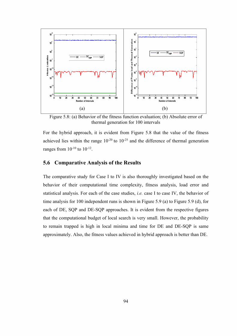
94
(a)
(b)
Figure 5.8: (a) Behavior of the fitness function evaluation; (b) Absolute error of thermal generation for 100 intervals
For the hybrid approach, it is evident from Figure 5.8 that the value of the fitness
achieved lies within the range 10-20 to 10-25 and the difference of thermal generation
ranges from 10-10 to 10-12.
5.6 Comparative Analysis of the Results
The comparative study for Case I to IV is also thoroughly investigated based on the
behavior of their computational time complexity, fitness analysis, load error and
statistical analysis. For each of the case studies, i.e. case I to case IV, the behavior of
time analysis for 100 independent runs is shown in Figure 5.9 (a) to Figure 5.9 (d), for
each of DE, SQP and DE-SQP approaches. It is evident from the respective figures
that the computational budget of local search is very small. However, the probability
to remain trapped is high in local minima and time for DE and DE-SQP is same
approximately. Also, the fitness values achieved in hybrid approach is better than DE.

95
Table 5.7: Comparative study in DE, SQP, and DE-SQP in terms of fitness achieved
Case
Study Solver Min Max Mean STD Var Mode
1
DE 0.0000E+00 0.0000E+00 0.0000E+00 0.0000E+00 0.0000E+00 0.0000E+00
SQP 1.2374E-12 1.2374E-12 1.2374E-12 6.0890E-28 3.7076E-55 1.2374E-12
DE-
SQP 0.0000E+00 1.1058E-11 1.2374E-12 2.4940E-12 6.2200E-24 0.0000E+00
2
DE 0.0000E+00 0.0000E+00 0.0000E+00 0.0000E+00 0.0000E+00 0.0000E+00
SQP 8.8948E-16 8.8948E-16 8.8948E-16 0.0000E+00 0.0000E+00 8.8948E-16
DE-
SQP 0.0000E+00 2.4514E-13 8.8948E-16 9.2651E-14 8.5842E-27 0.0000E+00
3
DE 0.0000E+00 0.0000E+00 0.0000E+00 0.0000E+00 0.0000E+00 0.0000E+00
SQP 8.7560E-14 2.2660E-12 2.1721E-12 3.0447E-13 9.2704E-26 2.2656E-12
DE-
SQP 7.7525E-17 7.6447E-13 4.3402E-13 1.8722E-13 3.5052E-26 7.7525E-17
4
DE 3.3162E+06 6.0206E+06 4.4814E+06 5.3298E+05 2.8407E+11 3.3162E+06
SQP 3.3087E-24 3.3087E-24 3.3087E-24 0.0000E+00 0.0000E+00 3.3087E-24
DE-
SQP 1.6466E-15 8.3930E-12 3.3087E-24 2.6583E-12 7.0667E-24 1.6466E-15
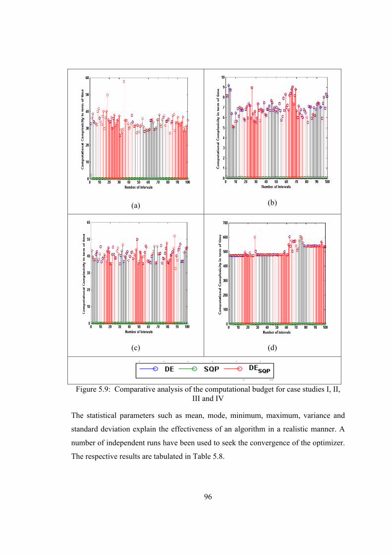
96
(a)
(b)
(c)
(d)
Figure 5.9: Comparative analysis of the computational budget for case studies I, II,
III and IV
The statistical parameters such as mean, mode, minimum, maximum, variance and
standard deviation explain the effectiveness of an algorithm in a realistic manner. A
number of independent runs have been used to seek the convergence of the optimizer.
The respective results are tabulated in Table 5.8.
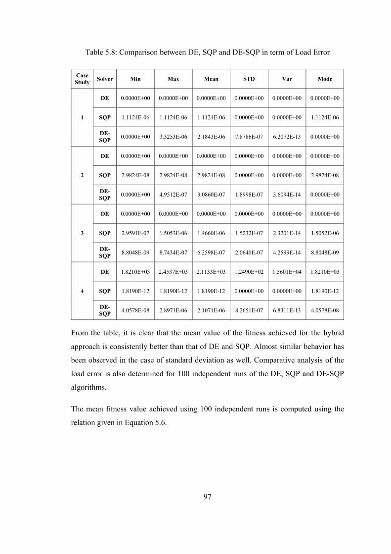
97
Table 5.8: Comparison between DE, SQP and DE-SQP in term of Load Error
Case Study Solver Min Max Mean STD Var Mode
1
DE 0.0000E+00 0.0000E+00 0.0000E+00 0.0000E+00 0.0000E+00 0.0000E+00
SQP 1.1124E-06 1.1124E-06 1.1124E-06 0.0000E+00 0.0000E+00 1.1124E-06
DE-SQP 0.0000E+00 3.3253E-06 2.1843E-06 7.8786E-07 6.2072E-13 0.0000E+00
2
DE 0.0000E+00 0.0000E+00 0.0000E+00 0.0000E+00 0.0000E+00 0.0000E+00
SQP 2.9824E-08 2.9824E-08 2.9824E-08 0.0000E+00 0.0000E+00 2.9824E-08
DE-SQP 0.0000E+00 4.9512E-07 3.0860E-07 1.8998E-07 3.6094E-14 0.0000E+00
3
DE 0.0000E+00 0.0000E+00 0.0000E+00 0.0000E+00 0.0000E+00 0.0000E+00
SQP 2.9591E-07 1.5053E-06 1.4660E-06 1.5232E-07 2.3201E-14 1.5052E-06
DE-SQP 8.8048E-09 8.7434E-07 6.2598E-07 2.0640E-07 4.2599E-14 8.8048E-09
4
DE 1.8210E+03 2.4537E+03 2.1133E+03 1.2490E+02 1.5601E+04 1.8210E+03
SQP 1.8190E-12 1.8190E-12 1.8190E-12 0.0000E+00 0.0000E+00 1.8190E-12
DE-SQP 4.0578E-08 2.8971E-06 2.1071E-06 8.2651E-07 6.8311E-13 4.0578E-08
From the table, it is clear that the mean value of the fitness achieved for the hybrid
approach is consistently better than that of DE and SQP. Almost similar behavior has
been observed in the case of standard deviation as well. Comparative analysis of the
load error is also determined for 100 independent runs of the DE, SQP and DE-SQP
algorithms.
The mean fitness value achieved using 100 independent runs is computed using the
relation given in Equation 5.6.

98
(5.6)
Similarly, the comparative study for DE, SQP, and DE-SQP in term of computational
complexity for case study 1 to 4 is provided in Table 5.9 using the relation given in
equation 5.7.
(5.7)
Table 5.9: Comparison between DE, SQP, and DE-SQP in term of computational
complexity Case
Study Solver Min Max Mean STD Var Mode
1
DE 25.7830 57.6757 33.5441 4.4063 19.4158 25.7830
SQP 0.0337 2.1092 0.0672 0.2065 0.0426 0.0337
DE-SQP 25.7974 57.8232 33.5714 4.4207 19.416 25.7974
2
DE 5.0349 9.1769 6.8964 0.8990 0.8082 5.0349
SQP 0.0409 0.1612 0.0514 0.0137 0.0002 0.0409
DE-SQP 5.0569 9.2737 6.9402 0.912 0.8084 5.0772
3
DE 32.4815 51.7848 40.5578 3.6145 13.0643 32.4815
SQP 0.0610 0.2841 0.0938 0.0343 0.0012 0.0610
DE-SQP 32.54 52.0225 40.6578 3.6476 13.0654 32.54
4
DE 472.1110 604.7093 507.3392 39.0906 1528.0744 472.1110
SQP 0.4338 0.7292 0.4999 0.0569 0.0032 0.4338
DE-SQP 472.6688 606.6227 508.2392 39.3652 1528.15 472.6688
It is quite clear from Table 5.9 that the computational budget in term of time
complexity increases with the increase in a number of generators. An important
parameter is a cost, in US$, for the production of power in MW. In this regard, a
comparative study is also carried out for DE, SQP and DE-SQP algorithms. The
results are given in Table 5.10. The dominance of DE-SQP is observed in the Table
5.10 as the mean value of the cost for DE-SQP is lower than that of global search
scheme and local search algorithm individually.
MF = 1ℜ
1N
fval − f̂valk
k=1
N
∑2⎛
⎝⎜
⎞
⎠⎟j
j=1
ℜ
∑
MET = 1ℜ
ET j
j=1
ℜ
∑
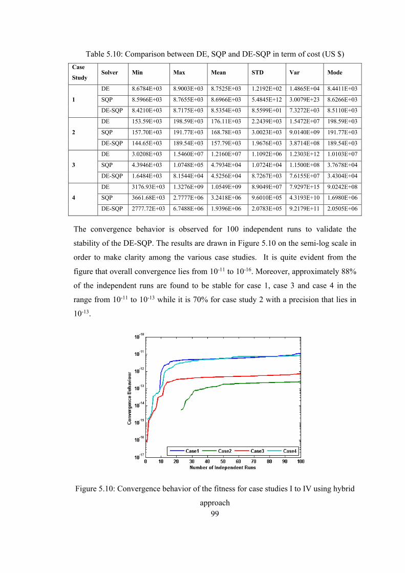
99
Table 5.10: Comparison between DE, SQP and DE-SQP in term of cost (US $) Case
Study Solver Min Max Mean STD Var Mode
1
DE 8.6784E+03 8.9003E+03 8.7525E+03 1.2192E+02 1.4865E+04 8.4411E+03
SQP 8.5966E+03 8.7655E+03 8.6966E+03 5.4845E+12 3.0079E+23 8.6266E+03
DE-SQP 8.4210E+03 8.7175E+03 8.5354E+03 8.5599E+01 7.3272E+03 8.5110E+03
2
DE 153.59E+03 198.59E+03 176.11E+03 2.2439E+03 1.5472E+07 198.59E+03
SQP 157.70E+03 191.77E+03 168.78E+03 3.0023E+03 9.0140E+09 191.77E+03
DE-SQP 144.65E+03 189.54E+03 157.79E+03 1.9676E+03 3.8714E+08 189.54E+03
3
DE 3.0208E+03 1.5460E+07 1.2160E+07 1.1092E+06 1.2303E+12 1.0103E+07
SQP 4.3946E+03 1.0748E+05 4.7934E+04 1.0724E+04 1.1500E+08 3.7678E+04
DE-SQP 1.6484E+03 8.1544E+04 4.5256E+04 8.7267E+03 7.6155E+07 3.4304E+04
4
DE 3176.93E+03 1.3276E+09 1.0549E+09 8.9049E+07 7.9297E+15 9.0242E+08
SQP 3661.68E+03 2.7777E+06 3.2418E+06 9.6010E+05 4.3193E+10 1.6980E+06
DE-SQP 2777.72E+03 6.7488E+06 1.9396E+06 2.0783E+05 9.2179E+11 2.0505E+06
The convergence behavior is observed for 100 independent runs to validate the
stability of the DE-SQP. The results are drawn in Figure 5.10 on the semi-log scale in
order to make clarity among the various case studies. It is quite evident from the
figure that overall convergence lies from 10-11 to 10-16. Moreover, approximately 88%
of the independent runs are found to be stable for case 1, case 3 and case 4 in the
range from 10-11 to 10-13 while it is 70% for case study 2 with a precision that lies in
10-13.
Figure 5.10: Convergence behavior of the fitness for case studies I to IV using hybrid
approach
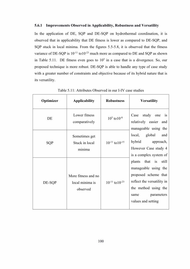
100
5.6.1 Improvements Observed in Applicability, Robustness and Versatility
In the application of DE, SQP and DE-SQP on hydrothermal coordination, it is
observed that in applicability that DE fitness is lower as compared to DE-SQP, and
SQP stuck in local minima. From the figures 5.5-5.8, it is observed that the fitness
variance of DE-SQP is 10-11 to10-23 much more as compared to DE and SQP as shown
in Table 5.11. DE fitness even goes to 105 in a case that is a divergence. So, our
proposed technique is more robust. DE-SQP is able to handle any type of case study
with a greater number of constraints and objective because of its hybrid nature that is
its versatility.
Table 5.11: Attributes Observed in our I-IV case studies
Optimizer Applicability Robustness Versatility
DE Lower fitness
comparatively 105 to10-8
Case study one is
relatively easier and
manageable using the
local, global and
hybrid approach,
However Case study 4
is a complex system of
plants that is still
manageable using the
proposed scheme that
reflect the versatility in
the method using the
same parameters
values and setting
SQP
Sometimes get
Stuck in local
minima
10-11 to10-15
DE-SQP
More fitness and no
local minima is
observed
10-11 to10-23

101
5.6.2 Efficiency of the Proposed Algorithm
DE-SQP is more efficient with respect to DE and SQP that can be observed from the
Table 5.12. In four cases two times DE struck in local optima as it is clear in the mean
value efficiency column.
Table 5.12: Efficiency of the Proposed Algorithm
Case Study
% of Efficiency % of Efficiency (Min Cost in $) (Mean Cost in $)
DE-SQP vs DE DE-SQP vs SQP DE-SQP vs DE DE-SQP vs SQP
1 3% 2% 2% 2% 2 6% 8% 10% 7% 3 45% 62% 9% 6% 4 13% 24% 13% 40%
5.7 Multi-objective Case Study
Here, four steam power plants, two combined heat and one is only heat plant. This
case study is taken from [17, 157]. The total power and heat demands are 600MW
and 150MWth respectively. Objectives of the study are minimization of fuel cost and
emission reduction. We have used Pareto Function to find the results of conflicting
objectives. Objective 1 is taken as cost minimization and objective 2 is taken as
emission minimization. Pareto front is shown in Fig 5.11. Values of Power and heat
taken from the plants are given in Table 5.13.

102
Table 5.13: Power and heat values in case of extreme objectives
Plants
DE-SQP F1,F2=[1,0]
Power in MW and heat in MWth
DE-SQP F1,F2=[0,1]
Power in MW and heat in MWth
P1 71.18196206 42.63799491
P2 98.53981394 48.51623351
P3 174.9971518 59.59845054
P4 124.9079094 83.56406851
P5 93.37306534 247
P6 44.00009743 125.6832525
H5 32.51221228 6.21E-23
H6 75.80518747 26.97321355
H7 41.68260025 123.0267864
Cost ($) 10352 17996
Emission (kg) 28.43 6.6

103
Figure 5.11: Pareto Front for Multi-objective Case Study
Hereby, the results of our proposed technique are compared with [17] and [147], for
better understanding of percentage of decrease in cost and emission with the related
work. DE-SQP saves 20% and 42% cost respectively as compard to [17] and [147],
as is evident in Table 5.14.
Table 5.14: Percentage of decrease of Cost and Emission
Methods Demand (MW)
Cost ($) (Cost)
Emission (Kg)
% Decrease Cost Emission
Proposed 1600 10352.36 6.6064 - - Lexicography
[17] 1600 12,908.90 14.572 19.69599
54.66374
SGA-II [147] 1600 17749.31 16.9208 41.67531
60.95693

104
5.8 Chapter Conclusion
Based on the simulation results, major findings are as follow:
• The stochastic optimizer based on Chaotic Differential Evolution - Sequential
Quadratic Programming (DE-SQP) and the hybrid scheme provide an alternate
platform to optimize Hydrothermal Coordination.
• The fitness value obtained by the DE-SQP outperforms that of DE and SQP
schemes. Similarly, the cost per MW of DE-SQP is lower when compared to
other optimizers.
• The fitness value for case-studies 1, 2, 3 and 4 lie in the following ranges:10-11
to 10-13; 10-12 to 10-15; 10-12 to 10-16; and 10-20 to 10-25.
• The convergence of the proposed scheme is validated through Monte Carlo
simulations. It has been observed from the graphs that the convergence
percentage for DE-SQP, SQP and DE is 100, 90 and 95 respectively.
• The computational complexity of DE-SQP is slightly higher than that of DE
and SQP. However, this effect can be overshadowed by the cost of supremacy
in DE-SQP absolute error.
• Another advantage of the proposed scheme is its simplicity, ease of
implementation, good convergence and accuracy.

105
6 Conclusion

106
6.1 Conclusion
The research endeavor deals with the topic of power plant planning from the
perspectives of planning as well as operations. It includes theoretical background,
mathematical problem formulation, and framework design, etc. Both short-term, as
well as long-term facets of power system planning, are presented. The work considers
non-linearity and realistic attributes to devise solutions. The thesis is a novel
contribution to the area of hybrid intelligent computational techniques and aims to
counter the complexities of Hydrothermal Coordination. The efficient Hydrothermal
Coordination scheme has various applications owing to its versatility and robustness.
This chapter summarizes the major findings of the research work, which are as
follows:
• Energy is an indispensable commodity and its importance can never be
ignored. Our work presents a comprehensive study of alternatives in power
generation. As a parameter, Levelized Cost of Electricity (LCOE) is consulted
to come forth with a viable solution. Various existing models are compared. It
has also been found that in order to reap maximum benefits, the strategy must
encourage the utilization of indigenous resources and localization of
technology.
• A multi-pronged approach needs to be adopted to assure emission
minimization and energy prosperity simultaneously: fossil-fueled power plants
subsidies should be withdrawn immediately in favor of subsidies to renewable
energy plants; a carbon tax regime should be implemented; in addition to
global and national, eco-friendly initiatives should be adopted on the domestic
scale as well.
• There are several constraints associated with Hydro-thermal Scheduling
(HTS), or Hydrothermal Coordination. For instance, it requires the power
generation to be equal to the power demand. Major factors that need to be
addressed, therefore, include reliability maximization, weather variations, and
resource control, etc. HTC is a highly complex, non-linear, non-deterministic,

107
multi-constrained, and dynamic optimization problem. It blends Economic
Dispatch (ED) and Unit Commitment (UC). Also, the search space of
Hydrothermal Coordination is non-linear and turbulent.
• Forecasting the resource and addressing the complexity are two of the main
focuses of Long-term Hydrothermal Coordination (LTHTC). A case study
about a local power project is considered for investigation purposes.
Intelligent computation for the optimal trade-off is carried out using Particle
Swarm Optimization (PSO). Markov Chain, a stochastic prediction model,
is used to predict the water inflow of Ghazi Barotha Hydropower Plant.
Moreover, we implemented Particle Swarm Optimization (PSO) algorithm to
handle the disparate problems and to assign unique weightage to each of the
objectives. This has, in turn, led us to come forth with the optimum utilization
of resources in the conflicting nature of objectives.
• While dealing with Short-term Hydrothermal Coordination (STHTC), the
evolutionary algorithms option promises the issue redressal in a versatile and
reliable manner. A viable global optimizer, based on Chaotic Differential
Evolution (CDE), is combined with Sequential Quadratic Programming
(SQP), an efficient local search technique. A multi-objective optimization
framework is established for minimizing the total cost of thermal generators
with valve-point loading effects. This results in an efficient Short-term
Hydrothermal Coordination (STHTC) scheme.
• Our scheme demonstrates to be superior when compared to extant
counterparts. In the application of DE, SQP and DE-SQP on hydrothermal
coordination, it is observed that DE fitness is lower as compared to DE-SQP,
and SQP is stuck in local minima. Further, it has been found that the fitness
variance of DE-SQP is 10-11 to 10-23 much better as compared to DE and
SQP. From the case studies, we found that the hybrid improved technique is
more robust as compared to individual techniques and avoids the divergence.
DE-SQP is able to handle any type of case study with a greater number of
constraints and objectives because of its hybrid nature that is its versatility. In

108
comparison to Differential Evolution, our proposed technique demonstrates to
be efficient within the range of 3% to 45%. And, when compared to
Sequential Quadratic Programming, our proposed technique showed efficiency
within the range of 2% to 62%.
• Our proposed scheme is far more efficient when compared to Lexicography
and SGA-II. The fuel consumption can be minimized by using cogeneration
plants and combined heat plants. In the scenario of a multi-objective case
study, a cogeneration case study is selected. The objectives of the study are
minimization of fuel cost as well as emission by meeting the heat requirement
as well as power demand. The results of our proposed technique are compared
with recent techniques of Lexicography and SGA-II, for better understanding
of the percentage of decrease in cost and emission with the related work. DE-
SQP saves 20% and 42% cost as compared to Lexicography and SGA-II
respectively. In terms of emission minimization, our proposed technique offers
savings of up to 55% and 61% when compared to Lexicography and SGA-II
respectively. We have considered only one objective at a time either cost
minimization or emission reduction. Pareto Function is also used to verify the
convergence of the technique.
6.2 Future Work
Undoubtedly, innovation in research and development is a never-ceasing process. Hydrothermal Coordination is no exception. In the future, as a follow-up of our research work, novel nature-inspired methods can be used to come forth with intelligent solutions aimed at more accuracy, less cost, and emission. The constraints relating to manpower, the uncertainty of the power plant (forecasting, generation, operation, financial) and other real-time parameters may be added in the mathematical modeling of STHTC and LTHTC systems along with viable linear and nonlinear metrics. The penetration of emerging technologies in daily lives is rapidly increasing. Energy modeling studies can be carried out to come forth with decreased complexity and assured outcomes. Moreover, future Hydrothermal Coordination solutions are reckoned to adopt a transdisciplinary approach by incorporating data science, artificial intelligence, and blockchain, etc.
109
7 References [1] M. T. Van Vliet, J. R. Yearsley, F. Ludwig, S. Vögele, D. P. Lettenmaier, and
P. Kabat, "Vulnerability of US and European electricity supply to climate change," Nature Climate Change, vol. 2, pp. 676-681, 2012.
[2] M. Afzal and M. K. Madhav, "Economic Load Dispatch and Unit Commitment Solution Using Advanced Optimization approach-A Review."
[3] A. S. Manne and R. G. Richels, "CO2 emission limits: an economic cost analysis for the USA," The Energy Journal, pp. 51-74, 1990.
[4] A. Mahari and K. Zare, "A solution to the generation scheduling problem in power systems with large-scale wind farms using MICA," International Journal of Electrical Power & Energy Systems, vol. 54, pp. 1-9, 2014.
[5] T. T. Nguyen, D. N. Vo, and A. V. Truong, "Cuckoo search algorithm for short-term hydrothermal scheduling," Applied Energy, vol. 132, pp. 276-287, 2014.
[6] S. Pereira, P. Ferreira, and A. Vaz, "Short-term electricity planning with increase wind capacity," Energy, vol. 69, pp. 12-22, 2014.
[7] R. Jiang, M. Zhang, G. Li, and Y. Guan, "Two-stage network constrained robust unit commitment problem," European Journal of Operational Research, vol. 234, pp. 751-762, 2014.
[8] P. González, J. Villar, C. A. Díaz, and F. A. Campos, "Joint energy and reserve markets: Current implementations and modeling trends," Electric Power Systems Research, vol. 109, pp. 101-111, 2014.
[9] J. Zábojník and M. Dvořák, "Power grid simulation model for long term operation planning," Applied Thermal Engineering, vol. 70, pp. 1294-1305, 2014.
[10] M. R. Norouzi, A. Ahmadi, A. E. Nezhad, and A. Ghaedi, "Mixed integer programming of multi-objective security-constrained hydro/thermal unit commitment," Renewable and Sustainable Energy Reviews, vol. 29, pp. 911-923, 2014.
[11] G. Ardizzon, G. Cavazzini, and G. Pavesi, "A new generation of small hydro and pumped-hydro power plants: advances and future challenges," Renewable and Sustainable Energy Reviews, vol. 31, pp. 746-761, 2014.
[12] M. Estahbanati, "Hybrid probabilistic-harmony search algorithm methodology in generation scheduling problem," Journal of Experimental & Theoretical Artificial Intelligence, vol. 26, pp. 283-296, 2014.
[13] E. Bakirtzis, P. N. Biskas, D. P. Labridis, and A. G. Bakirtzis, "Multiple time resolution unit commitment for short-term operations scheduling under high renewable penetration," Power Systems, IEEE Transactions on, vol. 29, pp. 149-159, 2014.
[14] Z. Zhou and A. Botterud, "Dynamic scheduling of operating reserves in co-optimized electricity markets with wind power," Power Systems, IEEE Transactions on, vol. 29, pp. 160-171, 2014.
[15] G. Steeger, L. A. Barroso, and S. Rebennack, "Optimal bidding strategies for hydro-electric producers: A literature survey," Power Systems, IEEE Transactions on, vol. 29, pp. 1758-1766, 2014.
[16] L. Martins, A. Azevedo, and S. Soares, "Nonlinear Medium-Term Hydro-Thermal Scheduling With Transmission Constraints," Power Systems, IEEE

110
Transactions on, vol. 29, pp. 1623-1633, 2014. [17] A. Ahmadi, M. R. Ahmadi, and A. E. Nezhad, "A lexicographic optimization
and augmented ϵ-constraint technique for short-term environmental/economic combined heat and power scheduling," Electric Power Components and Systems, vol. 42, pp. 945-958, 2014.
[18] J. Deane, E. McKeogh, and B. Gallachóir, "Derivation of intertemporal targets for large pumped hydro energy storage with stochastic optimization," Power Systems, IEEE Transactions on, vol. 28, pp. 2147-2155, 2013.
[19] K. Lakshmi and S. Vasantharathna, "Gencos wind–thermal scheduling problem using artificial immune system algorithm," International Journal of Electrical Power & Energy Systems, vol. 54, pp. 112-122, 2014.
[20] J. Zhou, X. Liao, S. Ouyang, R. Zhang, and Y. Zhang, "Multi-objective artificial bee colony algorithm for short-term scheduling of hydrothermal system," International Journal of Electrical Power & Energy Systems, vol. 55, pp. 542-553, 2014.
[21] W. Jiekang, G. Zhuangzhi, and W. Fan, "Short-term multi-objective optimization scheduling for cascaded hydroelectric plants with dynamic generation flow limit based on EMA and DEA," International Journal of Electrical Power & Energy Systems, vol. 57, pp. 189-197, 2014.
[22] K. Bhattacharjee, A. Bhattacharya, and S. H. nee Dey, "Oppositional real coded chemical reaction based optimization to solve short-term hydrothermal scheduling problems," International Journal of Electrical Power & Energy Systems, vol. 63, pp. 145-157, 2014.
[23] C. Wei, Z. M. Fadlullah, N. Kato, and A. Takeuchi, "GT-CFS: A game theoretic coalition formulation strategy for reducing power loss in micro grids," IEEE Transactions on Parallel and Distributed Systems, vol. 25, pp. 2307-2317, 2013.
[24] H. Tian, X. Yuan, B. Ji, and Z. Chen, "Multi-objective optimization of short-term hydrothermal scheduling using non-dominated sorting gravitational search algorithm with chaotic mutation," Energy Conversion and Management, vol. 81, pp. 504-519, 2014.
[25] R. Swain, A. Barisal, P. Hota, and R. Chakrabarti, "Short-term hydrothermal scheduling using clonal selection algorithm," International Journal of Electrical Power & Energy Systems, vol. 33, pp. 647-656, 2011.
[26] N. Fang, J. Zhou, R. Zhang, Y. Liu, and Y. Zhang, "A hybrid of real coded genetic algorithm and artificial fish swarm algorithm for short-term optimal hydrothermal scheduling," International Journal of Electrical Power & Energy Systems, vol. 62, pp. 617-629, 2014.
[27] B. Gjorgiev, D. Kančev, and M. Čepin, "A new model for optimal generation scheduling of power system considering generation units availability," International Journal of Electrical Power & Energy Systems, vol. 47, pp. 129-139, 2013.
[28] G. Sampaio, J. Saraiva, J. Sousa, and V. Mendes, "Optimization of the operation of hydro stations in market environment using Genetic Algorithms," in European Energy Market (EEM), 2013 10th International Conference on the, 2013, pp. 1-8.
[29] C. K. Simoglou, P. N. Biskas, S. I. Vagropoulos, and A. G. Bakirtzis, "Electricity market models and RES integration: The Greek case," Energy

111
Policy, vol. 67, pp. 531-542, 2014. [30] B. Mohammadi-Ivatloo, H. Zareipour, N. Amjady, and M. Ehsan,
"Application of information-gap decision theory to risk-constrained self-scheduling of GenCos," Power Systems, IEEE Transactions on, vol. 28, pp. 1093-1102, 2013.
[31] H. M. Pousinho, J. Contreras, A. G. Bakirtzis, and J. P. Catalao, "Risk-constrained scheduling and offering strategies of a price-maker hydro producer under uncertainty," Power Systems, IEEE Transactions on, vol. 28, pp. 1879-1887, 2013.
[32] B.-G. Koo, M.-S. Kim, K.-H. Kim, H.-T. Lee, J.-H. Park, and C.-H. Kim, "Short-term electric load forecasting using data mining technique," in Intelligent Systems and Control (ISCO), 2013 7th International Conference on, 2013, pp. 153-157.
[33] C. Batlle and P. Rodilla, "An enhanced screening curves method for considering thermal cycling operation costs in generation expansion planning," Power Systems, IEEE Transactions on, vol. 28, pp. 3683-3691, 2013.
[34] R. M. Lima, M. G. Marcovecchio, A. Queiroz Novais, and I. E. Grossmann, "On the computational studies of deterministic global optimization of head dependent short-term hydro scheduling," Power Systems, IEEE Transactions on, vol. 28, pp. 4336-4347, 2013.
[35] B. Tong, Q. Zhai, and X. Guan, "An MILP based formulation for short-term hydro generation scheduling with analysis of the linearization effects on solution feasibility," Power Systems, IEEE Transactions on, vol. 28, pp. 3588-3599, 2013.
[36] P. González, J. Villar, C. Diaz, and F. A. Campos, "Hourly energy and reserve joint dispatch with a hydro-thermal technological based representation," in European Energy Market (EEM), 2013 10th International Conference on the, 2013, pp. 1-8.
[37] K. Bruninx, D. Patteeuw, E. Delarue, L. Helsen, and W. D'haeseleer, "Short-term demand response of flexible electric heating systems: the need for integrated simulations," in European Energy Market (EEM), 2013 10th International Conference on the, 2013, pp. 1-10.
[38] A. Pina, C. A. Silva, and P. Ferrão, "High-resolution modeling framework for planning electricity systems with high penetration of renewables," Applied Energy, vol. 112, pp. 215-223, 2013.
[39] P. K. Roy, A. Sur, and D. K. Pradhan, "Optimal short-term hydro-thermal scheduling using quasi-oppositional teaching learning based optimization," Engineering Applications of Artificial Intelligence, vol. 26, pp. 2516-2524, 2013.
[40] E. C. Finardi and M. R. Scuzziato, "Hydro unit commitment and loading problem for day-ahead operation planning problem," International Journal of Electrical Power & Energy Systems, vol. 44, pp. 7-16, 2013.
[41] H. Zhang, J. Zhou, Y. Zhang, N. Fang, and R. Zhang, "Short term hydrothermal scheduling using multi-objective differential evolution with three chaotic sequences," International Journal of Electrical Power & Energy Systems, vol. 47, pp. 85-99, 2013.
[42] M. Parastegari, R.-A. Hooshmand, A. Khodabakhshian, and M. Vatanpour,

112
"AC constrained hydro-thermal generation scheduling problem: Application of Benders decomposition method improved by BFPSO," International Journal of Electrical Power & Energy Systems, vol. 49, pp. 199-212, 2013.
[43] R. Zhang, J. Zhou, and Y. Wang, "Multi-objective optimization of hydrothermal energy system considering economic and environmental aspects," International Journal of Electrical Power & Energy Systems, vol. 42, pp. 384-395, 2012.
[44] F. J. Díaz, J. Contreras, J. I. Muñoz, and D. Pozo, "Optimal scheduling of a price-taker cascaded reservoir system in a pool-based electricity market," Power Systems, IEEE Transactions on, vol. 26, pp. 604-615, 2011.
[45] X. Li and C. Jiang, "Short-term operation model and risk management for wind power penetrated system in electricity market," Power Systems, IEEE Transactions on, vol. 26, pp. 932-939, 2011.
[46] L. Xie, P. Carvalho, L. A. Ferreira, J. Liu, B. H. Krogh, N. Popli, et al., "Wind integration in power systems: Operational challenges and possible solutions," Proceedings of the IEEE, vol. 99, pp. 214-232, 2011.
[47] C. G. Baslis and A. G. Bakirtzis, "Mid-term stochastic scheduling of a price-maker hydro producer with pumped storage," Power Systems, IEEE Transactions on, vol. 26, pp. 1856-1865, 2011.
[48] K. K. Mandal and N. Chakraborty, "Optimal scheduling of cascaded hydrothermal systems using a new improved particle swarm optimization technique," Smart Grid and Renewable Energy, vol. 2, p. 282, 2011.
[49] C. Cheng, J. Shen, and X. Wu, "Short-term scheduling for large-scale cascaded hydropower systems with multivibration zones of high head," Journal of Water Resources Planning and Management, 2011.
[50] H. Vennila, T. R. D. Prakash, and T. Ruban, "A Solution for Environmental Constrained Economic Dispatch Problems using Honey Bee Algorithm," International Journal of Computer Applications, vol. 975, p. 8887, 2012.
[51] M. Basu, "Artificial immune system for fixed head hydrothermal power system," Energy, vol. 36, pp. 606-612, 2011.
[52] V. S. Kumar and M. Mohan, "A genetic algorithm solution to the optimal short-term hydrothermal scheduling," International Journal of Electrical Power & Energy Systems, vol. 33, pp. 827-835, 2011.
[53] M. Balasubbareddy, "Multi-objective optimization in the presence of ramp-rate limits using non-dominated sorting hybrid fruit fly algorithm," Ain Shams Engineering Journal, vol. 7, pp. 895-905, 2016.
[54] A. Frangioni, C. Gentile, and F. Lacalandra, "Sequential Lagrangian-MILP approaches for unit commitment problems," International Journal of Electrical Power & Energy Systems, vol. 33, pp. 585-593, 2011.
[55] C. C. A. Rajan, "Hydro-thermal unit commitment problem using simulated annealing embedded evolutionary programming approach," International Journal of Electrical Power & Energy Systems, vol. 33, pp. 939-946, 2011.
[56] K. Singh, N. Padhy, and J. Sharma, "Congestion management considering hydro–thermal combined operation in a pool based electricity market," International Journal of Electrical Power & Energy Systems, vol. 33, pp. 1513-1519, 2011.
[57] S. Sivasubramani and K. S. Swarup, "Hybrid DE–SQP algorithm for non-convex short term hydrothermal scheduling problem," Energy Conversion and
113
Management, vol. 52, pp. 757-761, 2011. [58] M. A. Crew, C. S. Fernando, and P. R. Kleindorfer, "The theory of peak-load
pricing: A survey," Journal of regulatory economics, vol. 8, pp. 215-248, 1995.
[59] L. F. Rangel, "Competition policy and regulation in hydro-dominated electricity markets," Energy Policy, vol. 36, pp. 1292-1302, 2008.
[60] H. Ge and S. Asgarpoor, "Reliability and maintainability improvement of substations with aging infrastructure," IEEE Transactions on Power Delivery, vol. 27, pp. 1868-1876, 2012.
[61] S. Shamugavel, "Reliability driven resource Scheduling algorithms for grid Computing," 2014.
[62] S. Zharkov, "Assessment and Enhancement of the Energy Supply System Efficiency with Emphasis on the Cogeneration and Renewable as Main Directions for Fuel Saving," International Journal of Energy Optimization and Engineering (IJEOE), vol. 3, pp. 1-20, 2014.
[63] D. Pudjianto, C. Ramsay, and G. Strbac, "Virtual power plant and system integration of distributed energy resources," IET Renewable Power Generation, vol. 1, pp. 10-16, 2007.
[64] A. Hussain, M. Amin, R. Khan, and F. A. Chaudhry, "Optimal Allocation of Flexible AC Transmission System Controllers in Electric Power Networks," INAE Letters, pp. 1-24, 2018.
[65] H. L. Willis, "Analytical methods and rules of thumb for modeling DG-distribution interaction," in Power Engineering Society Summer Meeting, 2000. IEEE, 2000, pp. 1643-1644.
[66] S. Doty and W. C. Turner, Energy management handbook: Crc Press, 2004. [67] M. Ashari, W. Keerthipala, and C. V. Nayar, "A single phase parallely
connected uninterruptible power supply/demand side management system," IEEE Transactions on Energy Conversion, vol. 15, pp. 97-102, 2000.
[68] F. Emir, "Selecting Renewable Energy Sources for Small Island Using Analytical Hierarchy Process (AHP)," Eastern Mediterranean University (EMU)-Doğu Akdeniz Üniversitesi (DAÜ), 2014.
[69] F. Chaudhry, M. Amin, M. Iqbal, R. Khan, and J. Khan, "A novel chaotic differential evolution hybridized with quadratic programming for short-term hydrothermal coordination," Neural Computing and Applications, pp. 1-12, 2017.
[70] F. Ueckerdt, L. Hirth, G. Luderer, and O. Edenhofer, "System LCOE: What are the costs of variable renewables?," Energy, vol. 63, pp. 61-75, 2013.
[71] E. S. Rubin, C. Chen, and A. B. Rao, "Cost and performance of fossil fuel power plants with CO2 capture and storage," Energy policy, vol. 35, pp. 4444-4454, 2007.
[72] P. L. Joskow, "Comparing the costs of intermittent and dispatchable electricity generating technologies," American Economic Review, vol. 101, pp. 238-41, 2011.
[73] X. Ouyang and B. Lin, "Levelized cost of electricity (LCOE) of renewable energies and required subsidies in China," Energy Policy, vol. 70, pp. 64-73, 2014.
[74] H. Akbari, "Shade trees reduce building energy use and CO2 emissions from power plants," Environmental pollution, vol. 116, pp. S119-S126, 2002.

114
[75] S. J. Davis, K. Caldeira, and H. D. Matthews, "Future CO2 emissions and climate change from existing energy infrastructure," Science, vol. 329, pp. 1330-1333, 2010.
[76] R. S. Haszeldine, "Carbon capture and storage: how green can black be?," Science, vol. 325, pp. 1647-1652, 2009.
[77] D. Pearce, "The role of carbon taxes in adjusting to global warming," The economic journal, vol. 101, pp. 938-948, 1991.
[78] M. Asif and T. Muneer, "Energy supply, its demand and security issues for developed and emerging economies," Renewable and Sustainable Energy Reviews, vol. 11, pp. 1388-1413, 2007.
[79] J. J. L. Rodriguez, A. M. Prina, D. Acosta, M. Guerra, Y. Huang, K. Jacob, et al., "The Prevalence and Correlates of Frailty in Urban and Rural Populations in Latin America, China, and India: A 10/66 Population-Based Survey," Journal of the American Medical Directors Association, 2018.
[80] Q. Wang, X. Chen, A. N. Jha, and H. Rogers, "Natural gas from shale formation–the evolution, evidences and challenges of shale gas revolution in United States," Renewable and Sustainable Energy Reviews, vol. 30, pp. 1-28, 2014.
[81] K. Branker, M. Pathak, and J. M. Pearce, "A review of solar photovoltaic levelized cost of electricity," Renewable and sustainable energy reviews, vol. 15, pp. 4470-4482, 2011.
[82] L. Hirth, F. Ueckerdt, and O. Edenhofer, "Integration costs revisited–An economic framework for wind and solar variability," Renewable Energy, vol. 74, pp. 925-939, 2015.
[83] M. Cai, Y. Wu, H. Chen, X. Yang, Y. Qiang, and L. Han, "Cost‐Performance Analysis of Perovskite Solar Modules," Advanced Science, vol. 4, 2017.
[84] C. Clauser and M. Ewert, "The renewables cost challenge: Levelized cost of geothermal electric energy compared to other sources of primary energy–Review and case study," Renewable and Sustainable Energy Reviews, 2017.
[85] M. Taylor, K. Daniel, A. Ilas, and E. Y. So, "Renewable power generation costs in 2014," International Renewable Energy Agency: Masdar City, Abu Dhabi, UAE, 2015.
[86] A. Hazlehurst, "Economic analysis of solar power: Achieving grid parity," ed: Stanford, CA: Stanford graduate school of business, 2009.
[87] "IRENA.Renewable Power Generation Costs in 2017. Available online: http://www.irena.org/publications/2018/Jan/Renewable-power-generation-costs-in-2017."
[88] "Lazard. In Lazard’s Latest Annual Levelized Cost of Energy Analysis (LCOE 11.0). 2017. Available online: https://www.lazard.com/perspective/levelized-cost-of-energy-2017."
[89] S. Chu and A. Majumdar, "Opportunities and challenges for a sustainable energy future," nature, vol. 488, p. 294, 2012.
[90] A. Chambers and N. Nakicenovic, "World Energy Outlook 2008," ed: IEA/OECD, 2008.
[91] I. I. E. Association, "World energy outlook 2009," ed: IEA, Paris, 2006. [92] F. Birol, "World energy outlook 2010," International Energy Agency, vol. 1,
2010. [93] M. v. Hoeven, "World energy outlook 2011," International Energy agency,
115
2011. [94] M. Van der Hoeven, "World energy outlook 2012," International Energy
Agency, Tech. Rep. ISBN, vol. 1033656550, 2012. [95] P. Olejarnik, "World energy outlook 2013," International Energy Agency:
France, 2013. [96] N. Scenario, M. East, and P. Cedex, "World energy outlook 2014 factsheet,"
Paris: International Energy Agency, 2015. [97] B. Fatih, "World energy outlook 2015," International Energy Agency, p. 1,
2015. [98] B. Obama, "The irreversible momentum of clean energy," Science, vol. 355,
pp. 126-129, 2017. [99] IEA., World Energy Outlook 2017: Organisation for Economic Co-operation
and Development, OECD, 2017. [100] "World Bank World Development Indicators. Available at
http://data.worldbank. org/data-catalog/world-development-indicators.," Accessed 20 June (2018).
[101] "Lizzard Company. (2015, Nov.). Lizard’s levelized cost of energy analysis-version 9.0. [Online]. Available: https://www.lazard.com/media/2390/lazards-levelized-cost-of-energy-analysis-90.pdf."
[102] S. Jacobsson and A. Bergek, "Transforming the energy sector: the evolution of technological systems in renewable energy technology," Industrial and corporate change, vol. 13, pp. 815-849, 2004.
[103] S. Emeis, Wind energy meteorology: atmospheric physics for wind power generation: Springer, 2018.
[104] G. Mokryani, Y. F. Hu, P. Papadopoulos, T. Niknam, and J. Aghaei, "Deterministic approach for active distribution networks planning with high penetration of wind and solar power," Renewable Energy, vol. 113, pp. 942-951, 2017.
[105] M. A. Green, "Solar cells: operating principles, technology, and system applications," 1982.
[106] C. Bermann, "Impasses and controversies of hydroelectricity," Estudos avançados, vol. 21, pp. 139-153, 2007.
[107] W. E. Glassley, "Geothermal Energy, Geology and Hydrology of," Encyclopedia of Sustainability Science and Technology, pp. 1-13, 2017.
[108] M. Ram, M. Child, A. Aghahosseini, D. Bogdanov, A. Lohrmann, and C. Breyer, "A comparative analysis of electricity generation costs from renewable, fossil fuel and nuclear sources in G20 countries for the period 2015-2030," Journal of cleaner production, vol. 199, pp. 687-704, 2018.
[109] I. R. E. Agency, "Renewable Capacity Statistics," ed: International Renewable Energy Agency Abu Dhabi, 2017.
[110] C. Shearer, R. Fofrich, and S. J. Davis, "Future CO2 emissions and electricity generation from proposed coal‐fired power plants in India," Earth's Future, vol. 5, pp. 408-416, 2017.
[111] R. Lueken, K. Klima, W. M. Griffin, and J. Apt, "The climate and health effects of a USA switch from coal to gas electricity generation," Energy, vol. 109, pp. 1160-1166, 2016.
[112] W. C. d. S. Júnior, "Water and Energy Nexus under Climate Change Scenarios: Lessons from Brazil," New Water Policy & Practice, vol. 4, pp. 7-
116
18, 2018. [113] F. Benhmad and J. Percebois, "Photovoltaic and wind power feed-in impact on
electricity prices: The case of Germany," Energy policy, vol. 119, pp. 317-326, 2018.
[114] G. G. Emissions, "Comparison of Lifecycle Greenhouse Gas Emissions of Various Electricity Generation Sources."
[115] A. Mollah, S. Sattar, M. Hossain, A. Salahuddin, and H. Ar-Rashid, "Prospects of nuclear energy for sustainable energy development in Bangladesh," International Journal of Nuclear Energy Science and Engineering, vol. 5, p. 28, 2015.
[116] http://www.wapda.gov.pk/. [117] R. N. Hoffman and E. Kalnay, "Lagged average forecasting, an alternative to
Monte Carlo forecasting," Tellus A: Dynamic Meteorology and Oceanography, vol. 35, pp. 100-118, 1983.
[118] M.-S. Lee, B. Elango, and S. P. Schnaars, "The accuracy of the Conference Board's buying plans index: A comparison of judgmental vs. extrapolation forecasting methods," International Journal of Forecasting, vol. 13, pp. 127-135, 1997.
[119] F. Gagliardi, S. Alvisi, Z. Kapelan, and M. Franchini, "A probabilistic short-term water demand forecasting model based on the Markov Chain," Water, vol. 9, p. 507, 2017.
[120] A. J. Wood and B. F. Wollenberg, Power generation, operation, and control: John Wiley & Sons, 2012.
[121] N. J. Redondo and A. Conejo, "Short-term hydro-thermal coordination by Lagrangian relaxation: solution of the dual problem," IEEE Transactions on Power Systems, vol. 14, pp. 89-95, 1999.
[122] B. Gorenstin, N. Campodonico, J. Costa, and M. Pereira, "Stochastic optimization of a hydro-thermal system including network constraints," in Power Industry Computer Application Conference, 1991. Conference Proceedings, 1991, pp. 127-133.
[123] P.-H. Chen and H.-C. Chang, "Genetic aided scheduling of hydraulically coupled plants in hydro-thermal coordination," IEEE Transactions on Power Systems, vol. 11, pp. 975-981, 1996.
[124] I. Farhat and M. El-Hawary, "Optimization methods applied for solving the short-term hydrothermal coordination problem," Electric Power Systems Research, vol. 79, pp. 1308-1320, 2009.
[125] I. Farhat and M. El-Hawary, "Short-term hydro-thermal scheduling using an improved bacterial foraging algorithm," in Electrical Power & Energy Conference (EPEC), 2009 IEEE, 2009, pp. 1-5.
[126] J. Castro and J. A. González, "A nonlinear optimization package for long-term hydrothermal coordination," European Journal of Operational Research, vol. 154, pp. 641-658, 2004.
[127] P.-H. Chen, "Pumped-storage scheduling using evolutionary particle swarm optimization," IEEE Transactions on Energy Conversion, vol. 23, pp. 294-301, 2008.
[128] V. Hinojosa and C. Leyton, "Short-term hydrothermal generation scheduling solved with a mixed-binary evolutionary particle swarm optimizer," Electric Power Systems Research, vol. 92, pp. 162-170, 2012.
117
[129] X. Yuan, B. Cao, B. Yang, and Y. Yuan, "Hydrothermal scheduling using chaotic hybrid differential evolution," Energy Conversion and Management, vol. 49, pp. 3627-3633, 2008.
[130] D. N. Simopoulos, S. D. Kavatza, and C. D. Vournas, "An enhanced peak shaving method for short term hydrothermal scheduling," Energy conversion and management, vol. 48, pp. 3018-3024, 2007.
[131] S. Kumar and R. Naresh, "Efficient real coded genetic algorithm to solve the non-convex hydrothermal scheduling problem," International Journal of Electrical Power & Energy Systems, vol. 29, pp. 738-747, 2007.
[132] M. E. El-hawary and G. S. Christensen, "Functional optimization of common-flow hydro-thermal systems," IEEE Transactions on Power Apparatus and Systems, pp. 1833-1839, 1972.
[133] R. P. Thompson, "Weather sensitive electric demand and energy analysis on a large geographically diverse power system ߞApplication to short term hourly electric demand forecasting," IEEE Transactions on Power Apparatus and Systems, vol. 95, pp. 385-393, 1976.
[134] H. Happ, "Optimal power dispatchߞA comprehensive survey," IEEE Transactions on Power Apparatus and Systems, vol. 96, pp. 841-854, 1977.
[135] W. Uturbey and A. S. Costa, "Dynamic optimal power flow approach to account for consumer response in short term hydrothermal coordination studies," IET Generation, Transmission & Distribution, vol. 1, pp. 414-421, 2007.
[136] L. Lakshminarasimman and S. Subramanian, "Hydrothermal coordination using modified mixed integer hybrid differential evolution," International Journal of Energy Technology and Policy, vol. 5, pp. 422-439, 2007.
[137] H. Dashti, A. J. Conejo, R. Jiang, and J. Wang, "Weekly Two-Stage Robust Generation Scheduling for Hydrothermal Power Systems," 2016.
[138] L. Ferreira, T. Andersson, C. Imparato, T. Miller, C. Pang, A. Svoboda, et al., "Short-term resource scheduling in multi-area hydrothermal power systems," International Journal of Electrical Power & Energy Systems, vol. 11, pp. 200-212, 1989.
[139] H. Brannlund, J. Bubenko, D. Sjelvgren, and N. Andersson, "Optimal short term operation planning of a large hydrothermal power system based on a nonlinear network flow concept," IEEE Transactions on Power Systems, vol. 1, pp. 75-81, 1986.
[140] J. Tang and P. B. Luh, "Hydrothermal scheduling via extended differential dynamic programming and mixed coordination," IEEE Transactions on Power Systems, vol. 10, pp. 2021-2028, 1995.
[141] G.-X. Luo, H. Habibollahzadeh, and A. Semlyen, "Short-term hydro-thermal dispatch detailed model and solutions," IEEE Transactions on Power Systems, vol. 4, pp. 1452-1462, 1989.
[142] R. Bansal, "Optimization methods for electric power systems: An overview," International Journal of Emerging Electric Power Systems, vol. 2, 2005.
[143] H. Y. Yamin, "Review on methods of generation scheduling in electric power systems," Electric Power Systems Research, vol. 69, pp. 227-248, 2004.
[144] P. K. Singhal and R. N. Sharma, "Dynamic programming approach for solving power generating unit commitment problem," in Computer and Communication Technology (ICCCT), 2011 2nd International Conference on,

118
2011, pp. 298-303. [145] C. E. Zoumas, A. G. Bakirtzis, J. B. Theocharis, and V. Petridis, "A genetic
algorithm solution approach to the hydrothermal coordination problem," IEEE transactions on power systems, vol. 19, pp. 1356-1364, 2004.
[146] M. Ventosa, M. Rivier, A. Ramos, and A. García-Alcalde, "An MCP approach for hydrothermal coordination in deregulated power markets," in Power Engineering Society Summer Meeting, 2000. IEEE, 2000, pp. 2272-2277.
[147] M. Basu, "Improved differential evolution for short-term hydrothermal scheduling," International Journal of Electrical Power & Energy Systems, vol. 58, pp. 91-100, 2014.
[148] R. Gnanadass, P. Venkatesh, and N. P. Padhy, "Evolutionary programming based optimal power flow for units with non-smooth fuel cost functions," Electric power components and systems, vol. 33, pp. 349-361, 2004.
[149] C.-C. Kuo, "A novel coding scheme for practical economic dispatch by modified particle swarm approach," IEEE Transactions on Power Systems, vol. 23, pp. 1825-1835, 2008.
[150] M. P. Camargo, J. L. Rueda, I. Erlich, and O. Añó, "Comparison of emerging metaheuristic algorithms for optimal hydrothermal system operation," Swarm and Evolutionary Computation, vol. 18, pp. 83-96, 2014.
[151] R. Storn and K. Price, "Differential evolution–a simple and efficient heuristic for global optimization over continuous spaces," Journal of global optimization, vol. 11, pp. 341-359, 1997.
[152] R. E. Perez-Guerrero and J. R. Cedeno-Maldonado, "Economic power dispatch with non-smooth cost functions using differential evolution," in Proceedings of the 37th Annual North American Power Symposium, 2005., 2005, pp. 183-190.
[153] J. Ilonen, J.-K. Kamarainen, and J. Lampinen, "Differential evolution training algorithm for feed-forward neural networks," Neural Processing Letters, vol. 17, pp. 93-105, 2003.
[154] T. Krink, B. Filipic, and G. B. Fogel, "Noisy optimization problems-a particular challenge for differential evolution?," in Evolutionary Computation, 2004. CEC2004. Congress on, 2004, pp. 332-339.
[155] A. Kumar, "Power Economic Dispatch with Valve-Point Loading Effects and Multiple Fuels Using Chaotic Based Differential Evolution," THAPAR UNIVERSITY, PATIALA, 2011.
[156] J. Yadav, N. Patidar, J. Singhai, S. Panda, and C. Ardil, "A combined conventional and differential evolution method for model order reduction," Measurement, vol. 183, p. 15885, 2009.
[157] M. Basu, "Combined heat and power economic emission dispatch using nondominated sorting genetic algorithm-II," International Journal of Electrical Power & Energy Systems, vol. 53, pp. 135-141, 2013.