December 8, 2021

Economic Theories and Macroeconomic Reality?1

Francesca Loriaa, Christian Matthesb,∗, Mu-Chun Wangc2

aFederal Reserve Board3

bIndiana University4

cDeutsche Bundesbank5

Abstract6

Economic theories are often encoded in equilibrium models that cannot be directly estimated7

because they lack features that, while inessential to the theoretical mechanism that is central to8

the specific theory, would be essential to fit the data well. We propose an econometric approach9

that confronts such theories with data through the lens of a time series model that is a good10

description of macroeconomic reality. Our approach explicitly acknowledges misspecification11

as well as measurement error. We highlight in two applications that household heterogeneity12

greatly helps to fit aggregate data, independently of whether or not nominal rigidities are con-13

sidered.14

JEL classifications: C32, C50, E3015

Keywords: Bayesian Inference, Misspecification, Heterogeneity, VAR, DSGE16

? We thank the editor Yuriy Gorodnichenko and associate editor Boragan Aruoba, an anonymous referee, GianniAmisano, Christiane Baumeister, Joshua Chan, Siddhartha Chib, Thorsten Drautzburg, Thomas Drechsel, EdHerbst, Dimitris Korobilis, Elmar Mertens, Josefine Quast, Frank Schorfheide, and Mark Watson as well asseminar and conference participants at the NBER-NSF Seminar on Bayesian Inference in Statistics and Econo-metrics, Indiana University, the National University of Singapore, the Drautzburg-Nason workshop, CEF, IAAE,and the NBER Summer Institute for their useful comments and suggestions on earlier versions of the paper.The views expressed in this paper are solely the responsibility of the authors and should not be interpreted asreflecting the views of the Federal Reserve Board, the Federal Reserve System, the Deutsche Bundesbank, theEurosystem, or their staff.

∗ Corresponding author, E-mail address: matthesc@iu.edu

“Essentially, all models are wrong, but some are useful.”17

— George Box (Box and Draper, 1987)

18

“I will take the attitude that a piece of theory has only intellectual interest until it has been19

validated in some way against alternative theories and using actual data.”20

— Clive Granger (Granger, 1999)

1. Introduction21

Economists often face four intertwined tasks: (i) discriminate between competing theories that22

are either not specified to a degree that they could be easily taken to the data in the sense that23

the likelihood function implied by those theories/models would be severely misspecified, or24

it would be too costly to evaluate the likelihood function often enough to perform likelihood-25

based inference, (ii) find priors for multivariate time series models that help to better forecast26

macroeconomic time series, (iii) use these multivariate time series models to infer the effects of27

structural shocks, and (iv) estimate unobserved cyclical components of macroeconomic aggre-28

gates. We introduce a method that tackles issue (i), and provides tools to help with the second,29

third, and fourth tasks.30

To introduce and understand our approach, let us for simplicity assume we have two theories at31

hand. In order to use our approach, we assume that these theories, while they might generally32

have implications for different variables X1,t and X2,t , share a common set of variables which33

we call Xt . Each theory implies restrictions on a Vector Autoregression (VAR, Sims, 1980) for34

Xt . We can figure out what these restrictions are by simulating data from each theory, which is35

achieved by first drawing from the prior for each theory’s parameters, then simulating data from36

each theory, and finally estimating a VAR on Xt implied by each theory. Doing this repeatedly37

gives us a distribution of VAR parameters conditional on a theory - we interpret this as the prior38

for VAR coefficients implied by each theory.39

We want to learn about these theories by studying how close a VAR estimated on data is to these40

theory-implied VARs. Xt might not be directly observed, but we have access to data on other41

2

variables Yt that we assume are linked to the VAR variables Xt via an unobserved components42

model, in which we embed the VAR for Xt .1 To estimate our model and learn about which the-43

ory is preferred by the data, we turn our theory-based priors for the VAR into one mixture-prior44

for the VAR using a set of prior weights. We devise a Gibbs sampler that jointly estimates all45

parameters in our model, the unobserved components Xt , as well as the posterior distribution of46

the weights on our mixture prior. The update from prior weights on each theory to a posterior47

distribution of weights tells us about the relative fit of each theory, taking into account issues48

such as measurement error or omitted trends that are captured by the unobserved components49

structure of our time series model.50

Because we allow deviations of the VAR coefficients’ posterior from either theory-based prior,51

we explicitly acknowledge misspecification. In particular, because of this feature there is no52

need to augment equilibrium models with ad-hoc features that are not central to the theories of53

interest, but could be crucial to the likelihood-based fit of an equilibrium model.54

We use our approach to show that modeling heterogeneity across households substantially im-55

proves the fit of various economic theories by studying two scenarios: (i) a permanent income56

example where one of the theories features some agents that cannot participate in asset markets57

(they are ”hand-to-mouth” consumers), and (ii) a New Keynesian example where one of the58

models features the same hand-to-mouth consumers.59

In real models with heterogeneous households and aggregate shocks, a common finding is that60

heterogeneity does not matter substantially for aggregate dynamics - see for example the bench-61

mark specification in Krusell and Smith (1998). Recent models with both heterogeneous house-62

holds and nominal rigidities following Kaplan et al. (2018) can break this ’approximate aggre-63

gation’ result. This still leaves the question whether aggregate data is better described by a64

heterogeneous agent model or its representative agent counterpart. To make progress on this65

issue, we introduce the aforementioned hand-to-mouth consumer into two standard economic66

theories. For the New Keynesian model, we build on Debortoli and Galı (2018), who show that67

1 This assumption captures issues such as measurement error and the situation where the actual data Yt has a cleartrend, while the variables in the theories Xt do not.

3

a two agent New Keynesian model can already approximate a richer heterogeneous model in68

terms of many aggregate implications.2 In both applications we find that even a model with69

this relatively stark form of heterogeneity is substantially preferred by the data to its repre-70

sentative agent counterpart. This finding does thus not hinge on nominal rigidities: Even in71

our permanent income example, the model with heterogeneous agents is preferred, albeit by a72

smaller margin (the posterior mean of the weight on the two-agent version of that model is 0.65,73

whereas the posterior mean of the weight on the two agent version of the New Keynesian model74

varies from 0.88 to 1 depending on the exact specification).75

The idea to generate priors from equilibrium for statistical models such as VARs is not new.76

Ingram and Whiteman (1994) generate a prior based on a real business cycle model for a VAR.77

Del Negro and Schorfheide (2004) go further by showing one can back out the posterior dis-78

tribution of the parameters of interest for their model from the VAR posterior.3 Our interest is79

different from theirs: We want to distinguish between possibly non-nested models that could80

not or should not be taken to the data directly.81

By focusing on the difference between theory-implied VAR coefficients and VAR coefficients82

estimated from data, our approach is philosophically similar to indirect inference, where a83

theory-based model is estimated by bringing its implied coefficients for a statistical model as84

close as possible to the coefficients of the same statistical model estimated on real data. In fact,85

the initial application of indirect inference used VARs as statistical models (Smith, 1993).86

The interpretation of an economic model as a device to generate priors for a statistical model87

is in line with the ’minimal econometric interpretation’ of an equilibrium model that was put88

forth by Geweke (2010) (see also DeJong et al., 1996). We think of our models as narrative de-89

vices that can speak to the population moments encoded in VAR parameters. What sets us apart90

from Geweke (2010) is that we explicitly model mis-measurement and, at the same time, want91

2 Other papers that develop similarly tractable heterogeneous agent New Keynesian models include Bilbiie (2018)and the many references therein.

3 Similar ideas have been used in a microeconometric context by Fessler and Kasy (2019). Filippeli et al. (2020)also build a VAR prior based on an equilibrium model, but move away from the conjugate prior structure forthe VAR used by Del Negro and Schorfheide (2004).

4

to infer the best estimate of the true economic variable using information from all equilibrium92

models.93

Our approach is generally related to the literature on inference in misspecified equilibrium mod-94

els. Ireland (2004) adds statistical (non micro-founded) auto-correlated noise to the dynamics95

implied by his equilibrium model to better fit the data. To assess misspecification and improve96

upon existing economic models, Den Haan and Drechsel (2021) propose to add additional non-97

micro-founded shocks, while Inoue et al. (2020) add wedges in agents’ optimization problems98

(which generally improve the fit of macroeconomic models, as described in Chari et al., 2007).99

Canova and Matthes (2021) use a composite likelihood approach to jointly update parameter100

estimates and model weights for a set of equilibrium models. We share with all those papers101

the general view that equilibrium models are misspecified, but our goal is not to improve esti-102

mates of parameters within an equilibrium model (like the composite likelihood approach) or103

to directly build a better theory (like papers in the ’wedge’ literature), but rather to provide a104

framework which allows researchers to distinguish between various economic models and to105

construct statistical models informed by (combinations of) these theories. Our approach is also106

related to earlier work on assessing calibrated dynamic equilibrium models, such as Canova107

(1994), Watson (1993), and Gregory and Smith (1991).108

Another contribution of our paper is to propose a tractable new class of mixture priors for109

VARs. As such, our work is related to recent advances in prior choice for VARs such as Villani110

(2009) and Giannone et al. (2019). In particular, in our benchmark specification, we exploit the111

conjugate prior structure introduced in Chan (2021) and extend it to our mixture setting. This112

structure has the advantage that it can handle large VARs well. Mixture priors have been used113

to robustify inference by, for example, Chib and Tiwari (1991) and Cogley and Startz (2019).114

To incorporate a small number of specific features from an economic theory in a prior, one115

can adaptively change the prior along the lines presented in Chib and Ergashev (2009). In our116

context, we want to impose a broad set of restrictions from a number of theories instead. The117

mixture priors we introduce could also incorporate standard statistical priors for VARs such as118

the Minnesota prior as a mixture component (similar in spirit to the exercise in Schorfheide,119

5

2000), as well as several “models” that only incorporate some aspects of theories, interpreted120

as restrictions on structural VAR parameters as in Baumeister and Hamilton (2019).121

Finally, our framework is constructed to explicitly acknowledge limitations of both data and122

theories: We allow for various measurements of the same economic concepts to jointly inform123

inference about economic theories and we do not ask theories to explain low-frequency features124

of the data they were not constructed to explain. We accomplish the second feature by estimat-125

ing a VAR for deviations from trends, where we use a purely statistical model for trends, which126

we jointly estimate with all other parameters, borrowing insights from Canova (2014).127

Our work is also related to opinion pools (Geweke and Amisano, 2011), where the goal is to find128

weights on aggregate predictions of various possibly misspecified densities (see also Amisano129

and Geweke, 2017, Del Negro et al., 2016 and Waggoner and Zha, 2012).130

131

2. Econometric Framework132

Our methodology aims to incorporate prior information on relationships in the data from133

multiple models and, at the same time, to discriminate between these models. In practical134

terms, we build a mixture prior for a VAR of unobserved state variables (e.g., model-based135

measures of inflation, output gap, etc.), where each mixture component is informed by one136

specific economic theory (or equilibrium model). This VAR is embedded in a state space model137

to account for measurement issues. We first give a broad overview of our approach (i.e. the138

ingredients of our state space model) before going into the details of each step. A bird’s eye139

illustration of our approach can be found in Appendix A.140

Economic Theories141

Consider a scenario where a researcher has K theories or economic models at hand that could142

potentially be useful to explain aspects of observed economic data. However, the theories are143

not necessarily specified in such a way that we can compute the likelihood function and achieve144

a reasonable fit of the data. This could be because, for example, the exogenous processes145

6

are not flexible enough to capture certain aspects of the data, or there are no relatively ad-146

hoc features such as investment adjustment costs in the models. While these features could147

be added to a specific model, we think it is useful to provide a framework that can test these148

simpler equilibrium models directly on the data. Our framework is also useful in situations149

where nonlinearities in models are important and the evaluation of the likelihood function is not150

computationally feasible.151

What do we mean by a model? We follow the standard protocol in Bayesian statistics and call152

model i the collection of a prior distribution fi(θi) for the vector of deep parameters θi of model153

i and the associated distribution of the data conditional on a specific parameter vector fi(X ti |θi)154

(Gelman et al., 2013).4 For each of the K models, we only require that we can simulate from155

fi(θi) and fi(X ti |θi). In Section 3.2 we show how this idea can be easily extended to situations156

where a researcher might only want to impose certain implications of a given theory. The157

simulation from the models constitutes one block or module of our algorithm.158

Model-Based Priors for VARs159

Given simulations from each model, we construct a prior from a conjugate family for a VAR on160

a set of variables common across models, that is X t ∈ Xi,t , ∀i. The specific form of the prior for161

each mixture component is dictated by the practical necessity of using natural conjugate priors162

for our VAR, for which the marginal likelihood is known in closed form.5 This mapping from163

simulations to VAR priors is the second block or module of our approach.164

Macroeconomic Reality: Mixture Priors165

We exploit a well-known result from Bayesian statistics (Lee, 2012): If the prior for a model166

is a mixture of conjugate priors, then the corresponding posterior is a mixture of the conjugate167

posterior coming from each of the priors. The weights of the mixture will be updated according168

4 A superscript denotes the history of a variable up to the period indicated in the superscript.5 As will become clear in this section, in theory we could use non-conjugate priors for each mixture, but then we

would need to compute (conditional) marginal likelihoods for each parameter draw, a task that is infeasible inpractice due to the computational cost it would come with.

7

to the fit (marginal likelihood) of the VAR model with each mixture component as prior. To169

make our approach operational, we note that the marginal likelihood for all conjugate priors170

commonly used for VARs is known in closed form (Giannone et al., 2015; Chan, 2021). This is171

important because in the final module of our approach we embed our VAR into a Gibbs sampler172

for a state space model because we want to allow for multiple measurements for each economic173

variable (e.g. CPI and PCE-based measures of inflation).174

We first establish that indeed a mixture prior consisting of conjugate priors results in a mixture175

posterior of the conjugate posteriors. To economize on notation, we consider two theories here,176

but the extension to K > 2 theories is straightforward. We denote the VAR parameter vector177

by γ . Note that even though each equilibrium model has a unique parameter vector, there is178

only one parameter vector for the VAR. Our approach constructs a prior for this VAR parameter179

vector that encodes various economic theories.180

Before going into detail, it will be useful to explicitly state the definition of a natural conjugate181

prior (Gelman et al., 2013).182

183

Definition 2.1 (Natural Conjugate Prior). Consider a class F of sampling distributions p(y|γ)

and P a class of prior distributions. then the class P is conjugate for F if

p(γ|y) ∈P for all p(.|γ) ∈F and p(.) ∈P

A class P is natural conjugate if it is conjugate for a class of sampling distributions and has184

the same functional form as the likelihood function.185

Turning now to mixture priors, we start by defining the prior:

p(γ) = w1 p1(γ)+w2 p2(γ),

where p1(γ) and p2(γ) are both conjugate priors with prior mixture weights w1 and w2 = 1−w1.

We denote a generic vector of data by y.

8

The posterior with a two-component mixture prior is given by

p(γ|y) = p(y|γ)p(γ)p(y)

=p(y|γ)(w1 p1(γ)+w2 p2(γ))

p(y),

where p(y|γ)w1 p1(γ) can be rewritten as

p(y|γ)w1 p1(γ) = w1 p1(γ|y)︸ ︷︷ ︸∝p(y|γ)p1(γ)

∫p(y|γ)p1(γ)dγ︸ ︷︷ ︸≡ML1

,

and where ML1 is the marginal likelihood if one were to estimate the VAR with prior p1(γ)186

only. A corresponding equation holds for the second mixture component.187

The posterior is thus a weighted average of the posteriors that we would obtain if we used each188

conjugate prior individually:6189

p(γ|y) = w′1 p1(γ|y)+w′2 p2(γ|y), (1)

where w′i =wiMLi

∑2j=1 w jML j

, ∀i = 1,2 (2)

MLi =∫

fi(γ)p(y|γ)dγ (3)

Note that the expression shows how to easily construct draws from the mixture posterior: With190

probability w′1 draw from p1(γ|y) and with the complementary probability draw from p2(γ|y).191

Draws from both p1(γ|y) and p2(γ|y) are easily obtained because they are conjugate posteriors.192

We embed this idea in a Gibbs sampler where the VAR governs the dynamics of an unobserved193

vector of state variables. Hence the model probabilities will vary from draw to draw. We next194

discuss each module of our approach in more detail, moving backwards from the last to the first195

step of our procedure.196

6 The equivalence between mixture priors and posteriors weighted by posterior model probabilities also appearsin Cogley and Startz (2019).

9

2.1. Our Time Series Model - Macroeconomic Reality197

With this general result in hand, we turn to our specific time series model. We embed the

VAR described above in a more general time series model for two reasons. First, the mapping

from variables in an economic model to the actually observed data is not unique - we usually

have multiple measurements for the same economic concept. Should our models match in-

flation based on the CPI, PCE, or GDP deflator? Should the short-term interest rate in New

Keynesian models be the Federal Funds rate or the three-month treasury bill rate? Should we

use expenditure or income-based measures of real output (Aruoba et al., 2016)? To circumvent

these issues, we treat model-based variables Xt as latent variables for which we observe vari-

ous indicators Yt . Second, economic theories might not be meant to describe the full evolution

of macroeconomic aggregates, but rather only certain aspects. While this is generally hard to

incorporate in statistical analyses, there is one specific aspect of macroeconomic theories that

we can incorporate, namely that many theories are only meant to describe the business cycle

and not low frequency movement.7 We thus follow Canova (2014) and allow for unobserved

components that are persistent and not related to the economic theories we consider.8 Our time

series model is thus:

Yt = µ +AXt +Bzt +ut , (4)

Xt =J

∑j=1

C jXt− j + εt , (5)

zt = µz + zt−1 +wt (6)

7 A telltale sign of this in macroeconomics is that data and model outputs are often filtered before comparisons.8 We do not mean to imply that this model might not be misspecified along some dimensions. We think of it as a

good description of many features of aggregate time series (more so than the economic theories we consider).One could enrich it to include a third vector of unobserved components that captures seasonal components, forexample. We choose to use seasonally adjusted data in our empirical application instead.

10

where utiid∼ N(0,Σu) is a vector of measurement errors with a diagonal covariance matrix Σu

9,198

εtiid∼ N(0,Σε) and wt ∼ N(0,Σw).199

We assume that ut , εt , and wt are mutually independent. Xt can be interpreted as the cyclical200

component of the time series. The behavior of Xt is informed by economic theories via our201

construction of a mixture prior for C j and Σε . Notice that in the case where some model-based202

variables in the vector of latent states Xt have multiple measurements, the A matrix linking Xt203

to the observable indicators Yt will have zeros and ones accordingly. zt can be interpreted as204

the trend component of the time series. We allow for at most one random walk component per205

element of Xt so that various measurements of the same variables share the same low frequency206

behavior, as encoded in the selection matrix B.10207

More general laws of motion for zt can be incorporated, but in our specific application we use208

a random walk to capture low-frequency drift in inflation and the nominal interest rate.11 We209

allow for a non-zero mean µz in the random walk equation to model variables that clearly drift210

such as log per capita real GDP in our application. If theories do have meaningful implications211

for trends of observables (as in our permanent income example in Section 5), our approach212

can easily be modified by dropping zt from the model and directly using implications from the213

theories to allow for unit roots in the priors for equation (5) along the lines discussed below. In214

that case Xt would capture both the cycle and trend of our observables. µ captures differences215

in mean across various measurements of the same economic concept. Allowing for different216

measurements frees us from making somewhat arbitrary choices such as whether to base our217

analysis on CPI or PCE-based inflation only.218

9 We can allow this measurement error to be autocorrelated. This adds as many parameters to our system as thereare observables because it adds one AR coefficient per observable as long as we model each measurement erroras an autoregressive process of order 1. We do this as a robustness check in Section 5.

10 Technically, we use a dispersed initial condition for z0 and set the intercept in the measurement equation for onemeasurement per variable with a random walk trend to 0. That variable’s intercept is then captured by z0.

11 A similar random walk assumption for inflation is commonly made in DSGE models, which in these modelsthen imparts the same low frequency behavior in the nominal interest rate. The equilibrium models we considerin our New Keynesian empirical application do not have that feature.

11

Estimation via Gibbs Sampling219

We can approximate the posterior via Gibbs sampling in three blocks with the mixture prior for220

the VAR coefficients γ = (β ,Σε) in hand (the construction of which we describe below), where221

β = vec(C jJj=1). We focus here on an overview of the algorithm, details can be found in222

Appendix B. A Gibbs sampler draws parameters for a given block conditional on the parameters223

of all other blocks. One sweep through all blocks then delivers one new set of draws.224

1. First, we draw the unobserved states XT and zT , which we estimate jointly. This can be225

achieved via various samplers for linear and Gaussian state space systems (Durbin and226

Koopman, 2012).227

2. The second block consists of the parameters for the measurement equation µ , A, and228

Σu.12 We use a Gaussian prior for µ and the free coefficients in A (if any - A can be a229

fixed selection matrix as in our empirical application, just as B) and an Inverse-Gamma230

prior for each diagonal element of Σu, which allows us to draw from the conditional231

posterior for those variables in closed form.232

3. Finally, the VAR coefficients γ are drawn according to the algorithm for drawing from233

the mixture posterior outlined before (note that the conditional marginal likelihood that is234

needed for this algorithm is available in closed form for all conjugate priors we consider235

here). We have three options for drawing from a natural conjugate prior for γ when the236

marginal likelihood (conditional on the parameters in the other blocks) is known:237

(i) The Normal-inverse Wishart prior (Koop and Korobilis, 2010).238

(ii) A variant of that prior where Σε is calibrated (fixed) a priori as in the classical239

Minnesota prior (see again Koop and Korobilis, 2010).240

(iii) The prior recently proposed by Chan (2021) that breaks the cross-equation correla-241

tion structure imposed by the first prior.242

12 Throughout we assume that the unobserved state vector Xt has a mean of zero. In our simulations from theequilibrium models we will demean all simulated data.

12

We use (iii) as our benchmark as it allows for a more flexible prior for γ while at the243

same time putting enough structure on the prior densities to make prior elicitation (i.e.244

the mapping from our simulated data to the prior) reasonably straightforward. We use245

prior (ii) for robustness checks - we find prior (i) to be too restrictive for actual empirical246

use. Another advantage of the prior structure introduced in Chan (2021) is that it is247

explicitly set up to be able to deal with a large number of observables, which means that248

our approach can also be used with a large dimensional Xt if an application calls for this.249

2.2. Simulating From Equilibrium Models - Economic Theories250

We assume that all economic models admit the following recursive representation:251

Xi,t = Fi(Xi,t−1,εi,t ,θi), ∀i = 1, ...,K (7)

where Fi is the mapping describing the law of motion of the state variables and εt,i are the struc-252

tural shocks in model i at period t. We focus on simulating demeaned data to be consistent with253

our state space models where the law of motion for Xt has no intercept.13254

We require that we can simulate from (an approximation to) this recursive representation. The255

specific form of the approximation is not important per se, but should be guided by the economic256

question. If nonlinearities are important, researchers can use a nonlinear solution algorithm. We257

discuss the interplay of a nonlinear solution algorithm and our linear time series model in more258

detail in Section 3.1 below. Note that while solving models nonlinearly can be time consuming,259

this step of the algorithm can generally be carried out in parallel.260

It is important to understand the role of simulating data Xt from a DSGE model to generate261

VAR priors. The intuition is that a DSGE model, conditional on priors on the deep parameters262

of the model, imposes very specific restrictions on the interactions among its model-based vari-263

ables and, as such, it implies very specific contemporaneous and dynamic covariances as well264

13 We find it useful to assume that the dimension of εi,t is at least as large as the dimension of Xt to minimizethe risk of stochastic singularity in the next steps. One can add ”measurement error” to Xi,t to achieve this, forexample.

13

as volatilities in the simulated sample. Therefore, a researcher can capture this information by265

examining the relationships in the simulated sample (e.g., they can infer dynamic correlations266

between inflation and output or the sign of the response of hours worked to a TFP shock).267

For our algorithm, we need N draws from the DSGE prior fi(θi). For each of these draws, we268

simulate a sample of length T of the theory-based variables Xi,t , and then estimate a VAR on269

this simulated dataset. These N estimates of VAR parameters for each theory are then used to270

generate a prior for the VAR model, as we describe next.271

272

2.3. Generating VAR Priors from Simulated Data273

Mapping Economic Theories Into Macroeconomic Reality274

As a reminder, we have K models with parameter vector θi and associated prior fi(θi) we275

want to derive VAR priors from.14 For a given n-dimensional vector of observables Yt , we need276

a prior for the VAR coefficients γ and the residual covariance matrix Σu. We use a simulation-277

based approach to set our priors. This not only generalizes to non-linear DSGE models but also278

allows us to easily take parameter uncertainty into account.279

1. To start, we simulate R datasets of length T burn−in + T f inal = T . We then discard the280

initial T burn−in periods for each simulation to arrive at a sample size of T f inal .281

• We pick the number of simulated data sets R to be at least 2000 in our applications.282

We generally recommend to increase the number of simulations until the corre-283

sponding prior does not change anymore. Since simulating the equilibrium models284

and computing the prior parameters can be done largely in parallel, this approach is285

not time consuming. Our choice for T f inal is 25 percent of the sample size of the286

14 The prior could be degenerate for some elements of θ if the researcher was interested in calibrating someparameters. The prior could also be informed by a training sample along the lines outlined by Del Negro andSchorfheide (2008).

14

actual data.15287

• The choice of T f inal implicitly governs how tight the variance of each mixture com-288

ponent is. If desired, a researcher can easily add an ad-hoc scaling factor to increase289

the variances of each mixture component.290

• Notice that in the case where length of the simulated datatsets T f inal → ∞, VAR291

parameter uncertainty conditional on a specific value of the DSGE parameters θi292

will vanish, but since we allow for uncertainty about those DSGE parameters there293

can still be uncertainty about VAR parameters even if the simulated sample size294

grows very large.295

2. For each model/mixture component, we choose the prior mean for the coefficients in the296

VAR to be the average VAR estimate across all simulations for that specific model. For the297

free parameters in the prior variances for γ , we set the elements equal to the corresponding298

elements of the Monte Carlo variance across simulations. Similarly, we use the Monte299

Carlo mean and variances to select the inverse-Gamma priors for the variances of the300

one-step ahead forecast errors (details can be found in Appendix C).301

3. We use a VAR(2) for Xt in our empirical application. We choose a relatively small number302

of lags for parsimony, but show as a robustness check that using a VAR(4) instead gives303

very similar results, a practice we generally recommend.304

2.4. An Illustration305

To get a sense of how our approach works in practice, we consider a simple example with306

two key features. First, we assume that we directly observe Xt , so that the data is already cleaned307

of measurement error and stochastic trends, and we can thus focus only on the part of the Gibbs308

sampler with the mixture prior. Second, we assume that we only estimate one parameter in the309

15 For larger systems with either a larger dimension of Xt or a larger number of lags in the dynamics for Xt , werecommend to adjust this fraction for the standard reason that tighter priors are needed / preferred in largersystems. For example, later we use a robustness check where we use a VAR(4) instead of a VAR(2), which isour benchmark choice. In that case we double T f inal to be 50 percent of the actual sample size (which is in linewith the value chosen by Del Negro and Schorfheide, 2004) since we doubled the number of lags.

15

prior mixture block of the Gibbs sampler, which allows us to plot priors and posteriors easily.310

In the left panel of Figure 1, we consider an example where we have two priors (in blue),311

which we use to form the mixture prior (for simplicity we assume equal weights). These priors312

generally come from equilibrium models in our approach. What determines how the prior model313

weights are updated is the overlap between the likelihood and each mixture component, as can314

be seen in equation (3). While component 2 is favored in this example, component 1 still has315

substantial overlap with the likelihood and hence a non-negligible posterior weight. Note that316

even if the likelihood completely overlapped with component 2, component 1 could in general317

still receive non-zero weight because of the overlap between the two components of the prior318

mixture.319

Normal Posterior Tighter Posterior

-2 -1.5 -1 -0.5 0 0.5 1 1.5 20

0.1

0.2

0.3

0.4

0.5

0.6

0.7

0.8

0

0.05

0.1

0.15

0.2

0.25

0.3

0.35

0.4

mixture component 1

mixture component 2

likelihood

-2 -1.5 -1 -0.5 0 0.5 1 1.5 20

0.1

0.2

0.3

0.4

0.5

0.6

0.7

0.8

0

1

2

3

4

5

6

7

8

mixture component 1

mixture component 2

likelihood

Figure 1: Components of Mixture Prior and Posterior.

We next turn to a scenario where the likelihood has less variance, as depicted in the right320

panel of Figure 1. What becomes apparent is that even as the posterior variance goes to zero (as321

it generally will in our applications with an increasing sample size) the model weights might322

still not become degenerate. This is not a flaw of our approach, but requires some discussion323

as to how we think about asymptotic behavior in this framework. Traditionally, in a Bayesian324

context one might think about asymptotic behavior as letting the sample size grow to infinity325

without changing the prior. In order to be asymptotically able to discriminate with certainty326

16

between theories with our approach, we should increase the sample size used to simulate data327

from the equilibrium models to form the prior. This will lead to the mixture components having328

less overlap and hence making discriminating between models easier. Note that this does not329

mean that the variance of the mixture prior will go to zero. Our benchmark approach automati-330

cally sets the size of the simulations that determine the VAR prior to be a constant fraction (25331

percent) of the actual sample size.332

Insofar as cleaning the data of measurement error and stochastic trends (as we do with our Gibbs333

sampler) removes outliers or makes them less severe, our approach is more robust to outliers334

in the data than using the observed data to compute the marginal likelihoods of the economic335

models directly. This is due to the fact that our model weights are based on marginal likeli-336

hood comparisons for the VAR of the unobserved cyclical component vector Xt , and thus the337

likelihood function for Xt does not move as much in response to outliers (i.e., when outliers are338

added to the data set) as the likelihood function of the theoretical model when such a theoretical339

model does not take into account all the measurement and trend issues that we do.16340

3. Extensions341

In this section we are going to consider two important extensions of our procedure. The first342

extension considers the case where a researcher is interested in using our procedure to incor-343

porate information from nonlinear theories/models. The second shows how our methodology344

can be easily extended to the case where, instead of using fully specified economic theories,345

a researcher might be interested in imposing only certain implications of a theory while being346

agnostic about others. In Appendix D we also present a third extension, which describes how347

to estimate impulse responses via a data-driven approach to selecting among/averaging over348

identification schemes coming from different models/theories.349

16 By ”likelihood function for Xt” we mean the density of Xt conditional on parameters, as depicted, for example,in Figure 1.

17

3.1. Nonlinearities and the Choice of Variables350

While our time series model is linear, if the equilibrium models we study are solved using

nonlinear solution methods and nonlinearities are possibly important for discriminating between

theories, then our approach can exploit these nonlinearities. To highlight this point, consider a

simplified version of our setup where, instead of a VAR, we use a univariate linear regression

to discriminate among models:

x1,t = Ξx2,t + εt

where x1,t and x2,t are demeaned variables simulated from an equilibrium model. We know351

that asymptotically Ξ =cov(x1,t ,x2,t)

var(x2,t), where cov and var are population moments. Under well352

known conditions, the regression coefficient on long simulations from the model will approach353

Ξ. However, these population moments themselves will generally depend on the order of ap-354

proximation used to solve and simulate the equilibrium model. It is not true that a first-order355

approximation and a non-linear solution method will generically deliver similar values for Ξ,356

even though it is a regression coefficient in a linear regression and the decisions rules from a357

first-order approximation give the best linear approximation to the true nonlinear decision rules.358

If heterogeneity or movements in higher-order moments (such as standard deviations) are im-359

portant and a feature of all equilibrium models that are studied, then measures of cross-sectional360

dispersion or higher-order moments can be included in the time series model if data on these361

moments are available. We can then think of the time series model as a linear approximation to362

the joint dynamics of aggregate variables and these higher-order or cross-sectional moments.17363

3.2. Incorporating Only Some Aspects of Theories364

Our approach allows researchers to include only some aspects of economic theories while365

being agnostic about others by using structural VARs instead of fully specified economic theo-366

ries to form priors. This extension builds on Baumeister and Hamilton (2019), who show how367

to map beliefs about certain aspects of economic theories into a prior for a structural VAR. This368

17 Measures of higher order moments are, for example, commonly introduced in linear time series models to studythe effects of uncertainty shocks - see Bloom (2009).

18

prior information may come from simple or more articulated theoretical models and can be369

summarized as a set of restrictions on the structural VAR matrices. For instance, prior beliefs370

about the magnitude or sign of the impulse responses of a dependent variable to a shock (“oil371

production does not respond to the oil price, on impact” or “a TFP shock leads to increase in372

hours worked”) can be cast as priors on the impact matrix of the structural VAR model. For373

other features of the data, one can use non-informative or standard priors that are not directly374

linked to a fully specified economic theory. Aruoba et al. (2021) follow a similar logic in their375

structural VAR model in which an occasionally-binding constraint generates censoring in one376

of the dependent variables. In their application the censored variable is the nominal interest rate377

constrained by the effective lower bound and prior beliefs about directions of impulse responses378

are based on a simple New Keynesian DSGE model.379

Our framework can be used to embrace several of such “theories” by using a modified version of380

our algorithm. To see this, first consider the following structural VAR model, which represents381

one of our “theories”:382

Ai,0Xi,t = Ai,1Xi,t−1 +νi,t , (8)

where Xi,t is an (ni×1) vector of variables in model i, Ai,0 an (ni×ni) matrix describing con-383

temporaneous structural relations, Xi,t−1 a (ki×1) vector encompassing a constant and mi lags384

of Xi,t (and, thus, ki = mini + 1) and νi,t ∼N (0,Ωi,ν) is an (ni× 1) vector. As in Baumeis-385

ter and Hamilton (2019), prior information about Ai,0 in model i would be represented by the386

prior density fi(Ai,0) and may speak to individual elements of Ai,0 (e.g., restrictions on con-387

temporaneous relationships) or to its nonlinear combinations, such as elements of A −1i,0 (e.g.,388

restrictions on impulse responses). Priors on the other parameters could be informed by either389

economic theories or standard priors in the VAR literature (such as the Minnesota prior for Ai,1390

used in Baumeister and Hamilton, 2019).391

To apply our procedure to such a framework, one simply needs to draw the structural VAR392

parameters from their prior, simulate data Xi,t from model (8) conditional on these parameters,393

and then proceed with generating priors for the VAR parameters γ , before finally moving on to394

19

the “Macroeconomic Reality” step in our procedure (described in Section 2 and illustrated in395

Figure A-1 of Appendix A).396

4. Some Monte Carlo Examples397

To get a sense of how our approach performs and how it relates to standard measures of398

fit, we present a series of examples and associated Monte Carlo simulations. A first set of399

simulations highlights that our approach automatically provides model averaging or model dis-400

crimination based on the data-generating process. We do this using a setup with simple sta-401

tistical models. Afterwards, we study an economic example where the models available to the402

researcher are misspecified in economically meaningful ways. Another Monte Carlo example,403

which highlights the trade-off between small and large models and the role played by the choice404

of observables in that trade-off, can be found in Appendix F.405

4.1. Model Averaging and the Role of Measurement Error406

To show that our approach can be used not only to discriminate between models but also to407

optimally combine them when they are all useful representations of the data, we now consider408

a simulation exercise. Here we simulate one sample per specification for the sake of brevity,409

but the random seed is fixed across specifications, so the innovations in the simulated data410

are the same across simulates samples (only the endogenous propagation changes). In this411

specification, we study 200 observations of a scalar time series yt . We consider two models:412

Model 1. Less Persistence413

yt = 0.7yt−1 + et , (9)

where etiid∼ N(0,1), and414

Model 2. More Persistence415

yt = 0.9yt−1 + et , (10)

where again etiid∼ N(0,1). We consider three data-generating processes: One where the less416

persistent model is correct, one where the more persistent model is correct, and one where the417

20

DGP switches from the first model to the second in period 101 (the middle of the sample).18418

Table 1 shows that if models fit (part of) the data well, our approach will acknowledge this, as419

both models receive basically equal weight in the case of the third DGP, whereas the correct420

model dominates in the first two DGPs.421

Table 1: Posterior Mean of Model Weights, Second Simulation Exercise.

Data-Generating Process (Average Posterior) Weight of Model 1 Weight of Model 2

Model 1 is correct 0.89 0.11Model 2 is correct 0.17 0.83Switch in t = T/2 0.48 0.52

In this setup we can also assess the role of measurement error further. While measure-422

ment error can make it harder to discriminate among models in theory, our measurement error423

is restricted to be i.i.d. When we redo our analysis, but now introduce extreme measurement424

error (where for simplicity we fix the measurement error variance to be 1), the results are basi-425

cally unchanged. To give one example, if model 2 is the correct model and we allow for such426

measurement error in our estimated model (measurement error that is absent from the data-427

generating process), the model probability for model 2 is 0.91. Measurement error does not428

significantly move the estimated model weights because the difference across the two models429

is that model 2 is more persistent, which the iid measurement error cannot mask.430

4.2. Misspecified Frictions in a DSGE Model431

We now turn to the following scenario: Suppose the data-generating process is a LARGE432

equilibrium model with a substantial number of frictions. We simulate data from this model, but433

then compare two misspecified models: One model where one friction is turned off only, and434

another, smaller, model where other frictions are missing, but the one friction the first model435

gets wrong is actually present. As a laboratory, we use the Schmitt-Grohe and Uribe (2012)436

18 We use the standard Normal-inverse Wishart prior. We shut down the random walk component and assume weobserve a measurement of yt that is free of measurement error in the first three exercises.

21

real business cycle (RBC) model.19 This is a real model with a rich set of frictions to match US437

data. Schmitt-Grohe and Uribe (2012) study news shocks, but for simplicity we turn off these438

shocks in our exercises (so they are not present in neither the DGP nor the models we want to439

attach weights to).440

Our DGP adds one friction to the standard Schmitt-Grohe and Uribe (2012) model: A time441

varying discount factor, where time variation can be due to time variation in the capital stock442

or an exogenous shock. The specification we use for this time variation is due to Canova et al.,443

2020. Time variation in the discount factor has become a common tool to model, for example,444

sudden shifts in real interest rates - see for example Bianchi and Melosi (2017). The first model445

we consider is equal to the DGP except that it lacks time variation in the discount factor. The446

second model features this time variation, but lacks other frictions present in the DGP: Habits,447

investment adjustment costs, varying capacity utilization, and mark-up shocks. We simulate448

200 Monte Carlo samples of length 250. The parameter values of each model are calibrated449

for each simulated data set (so the priors fi(θi) are degenerate, which makes it easier for us to450

discuss misspecification).20 As observables we use consumption, hours, and investment.451

When we carry out this exercise, the result is not surprising: The larger model which only has452

one misspecification is clearly preferred by the data (average model weight of 1). What we are453

interested in, is how our model weights behave as we make the models closer to each other454

and if there are substantial differences relative to Bayesian model probabilities. To do so, we455

exploit that fact that each of the fractions that the smaller model is missing is governed by one456

parameter. We now reintroduce two of these frictions, habits in consumption and investment457

adjustment costs, but not using the true parameter values, but a common fraction x (with x < 1)458

of the true value. Table 2 shows the results for selected values of x. As we increase x, our459

approach realizes that both models provide useful features to match the data. Bayesian model460

probabilities of the equilibrium models themselves, on the other hand, suggest that only the461

19 In Appendix F, we use a New Keynesian model in another Monte Carlo exercise. In that exercise, we alsoextend our framework to allow for additional exogenous regressors in our VAR for Xt so that it can be used, forexample, to focus on implications for a single variable such as the nominal interest rate.

20 We discuss details of the calibration in Appendix E.

22

larger model is useful. Our approach is more cautious in that it tends to give positive weights462

to all available models, similarly to the opinion pools literature (Geweke and Amisano, 2011).463

This feature will also be present in our empirical examples later.21464

Table 2: Model Weights and Model Probabilities.

Model Specification (value of x) Our Approach Bayesian Model Probability

0.25 0.21 0.000.33 0.46 0.000.40 0.61 0.000.55 0.78 0.00

5. Does Heterogeneity Matter for Aggregate Behavior?465

A key question for anyone trying to write down a macroeconomic model is whether to466

include household heterogeneity. A traditional answer, using results from Krusell and Smith467

(1998), is that household heterogeneity might not matter for aggregate outcomes as much as we468

would think. In this section we highlight that this is not a general result by using two empirical469

applications: (i) a permanent income example, where we use aggregate US data on real income470

and consumption to distinguish between a representative agent permanent income model and471

a version of the same model that also has hand-to-mouth consumers, and (ii) a stylized three472

equation New Keynesian model where we again contrast the representative agent version with473

a version that also has hand-to-mouth households.474

These two examples share similarities (such as the use of hand-to-mouth consumers to introduce475

a stylized notion of household heterogeneity), but they also differ in important aspects: The476

permanent income example uses theories that have implications for trends. We therefore shut477

down the trends in our unobserved components model and instead allow for unit roots in the478

VAR for Xt .22 The New Keynesian application instead uses theories that only have implications479

21 In Appendix I, we provide a more detailed discussion of the differences between standard Bayesian modelprobabilities and our approach, in particular focusing on why our approach will likely lead to less extrememodel weights.

22 The first application also shuts down measurement error in the observation equation of our unobserved compo-nents model.

23

for cyclical behavior.480

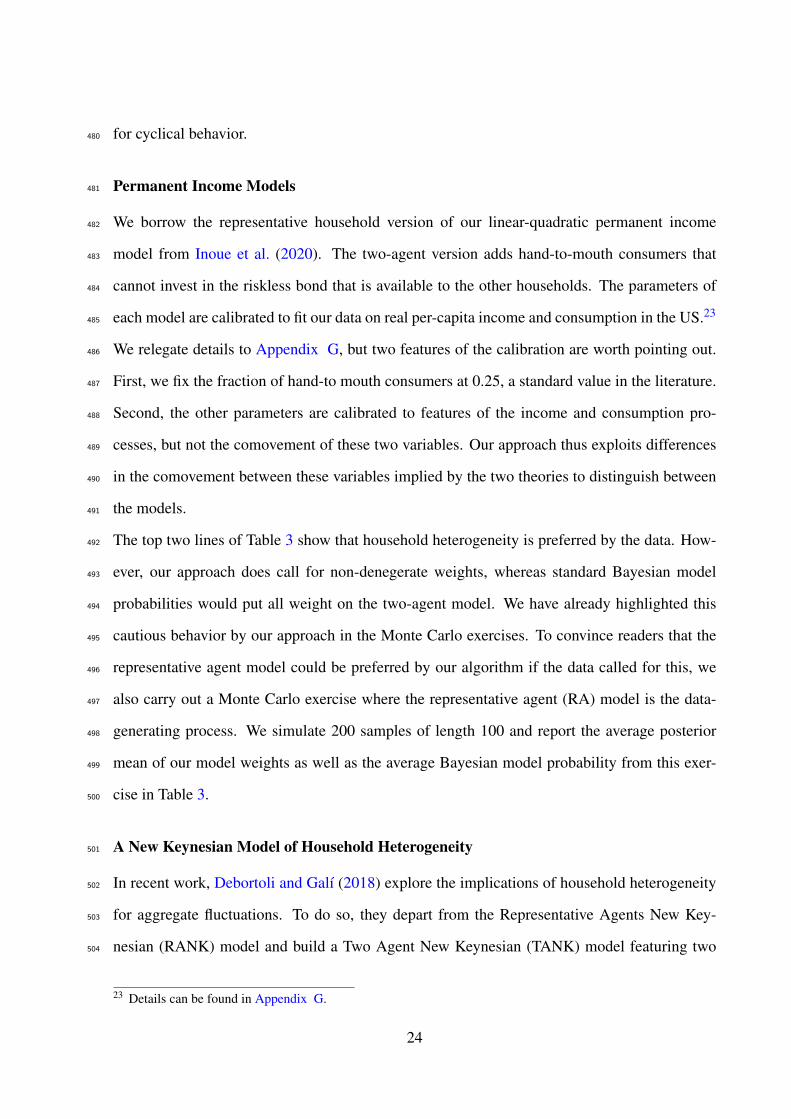
Permanent Income Models481

We borrow the representative household version of our linear-quadratic permanent income482

model from Inoue et al. (2020). The two-agent version adds hand-to-mouth consumers that483

cannot invest in the riskless bond that is available to the other households. The parameters of484

each model are calibrated to fit our data on real per-capita income and consumption in the US.23485

We relegate details to Appendix G, but two features of the calibration are worth pointing out.486

First, we fix the fraction of hand-to mouth consumers at 0.25, a standard value in the literature.487

Second, the other parameters are calibrated to features of the income and consumption pro-488

cesses, but not the comovement of these two variables. Our approach thus exploits differences489

in the comovement between these variables implied by the two theories to distinguish between490

the models.491

The top two lines of Table 3 show that household heterogeneity is preferred by the data. How-492

ever, our approach does call for non-denegerate weights, whereas standard Bayesian model493

probabilities would put all weight on the two-agent model. We have already highlighted this494

cautious behavior by our approach in the Monte Carlo exercises. To convince readers that the495

representative agent model could be preferred by our algorithm if the data called for this, we496

also carry out a Monte Carlo exercise where the representative agent (RA) model is the data-497

generating process. We simulate 200 samples of length 100 and report the average posterior498

mean of our model weights as well as the average Bayesian model probability from this exer-499

cise in Table 3.500

A New Keynesian Model of Household Heterogeneity501

In recent work, Debortoli and Galı (2018) explore the implications of household heterogeneity502

for aggregate fluctuations. To do so, they depart from the Representative Agents New Key-503

nesian (RANK) model and build a Two Agent New Keynesian (TANK) model featuring two504

23 Details can be found in Appendix G.

24

Table 3: Results, Permanent Income Models.

Model and Data Used Our Approach Bayesian Model Probabilities

One household, US data 0.35 0.00Two households, US data 0.65 1.00One household, RA model is DGP 0.75 0.69Two households, RA model is DGP 0.25 0.31

types of households, namely “unconstrained” and “constrained” households, where the type is505

respectively determined by whether a household’s consumption satisfies the consumption Eu-506

ler equation. A constant share of households is assumed to be constrained and to behave in a507

“hand-to-mouth” fashion in that they consume their current income at all times.508

Their framework shares a key feature with Heterogeneous Agents New Keynesian models509

(HANK): At any given point in time there is a fraction of households that faces a binding510

borrowing constraint and thus cannot adjust their consumption in response to changes in inter-511

est rates or any variable other than their current income. Relative to HANK models, the TANK512

framework offers greater tractability and transparency , but it comes at the cost of assuming a513

more stylized form of household heterogeneity. Nonetheless, Debortoli and Galı (2018) also514

show that TANK models approximate the aggregate output dynamics of a canonical HANK515

model in response to monetary and non-monetary shocks reasonably well.516

We use versions of these models to simulate data on log output, hours worked, real interest517

rate and productivity.24 The model equations as well as the priors over the deep parameters of518

the DSGE model can be found in Appendix H.1 and Appendix H.2. All DSGE priors (the519

fi(θi) distributions) are common across the two models except the prior for λ , the fraction of520

constrained households in the two-agent model. While this fraction is set to 0 in the RANK521

model, we use a truncated normal distribution which is truncated to be between 0.1 and 0.3 (the522

underlying non-truncated distribution has mean 0.2 and standard deviation 0.1). The priors for523

24 The only differences relative to Debortoli and Galı (2018) are that we use introduce a cost-push shock insteadof their preference shifter (to be comparable to most other small scale New Keynesian models), and that weuse a backward-looking monetary policy rule, which we found made the OLS-based VAR estimates based onsimulated data more stable.

25

those parameters that are not informed by the DSGE model are described in detail in Appendix524

H.3. The prior model weights are 0.5 each. As observables, we use quarterly log of per capita525

real GDP and GDI as measures of output, annualized quarterly CPI and PCE inflation, and the526

Federal Funds rate and the three months T-bill rate for the nominal interest rate. Our sample527

starts in 1970 and ends in 2019. More details on the data can be found in Appendix H.4.528

Both of these theories are very much stylized: They disregard trends in nominal and real vari-529

ables, the one theory that allows for heterogeneity does so in a stylized fashion, and the models530

will be approximated using log-linearization, thus disregarding any non-linearities. Nonethe-531

less, we will see below that the TANK model provides a better fit to the data series we study.532

We introduce random walk components for all three variables (output, inflation, and nominal533

interest rates). The different measurements for the same variables are restricted to share the534

same low-frequency random-walk components and the same cyclical components, but they can535

have different means and different high-frequency components. We use a larger prior mean for536

the innovation to the random walk in output compared to inflation and nominal interest rates537

to account for the clear trend. We allow for independent random walk components in inflation538

and the nominal interest rate to be flexible, but one could restrict those variables to share the539

same trend (as would be implied by equilibrium models with trend inflation described by, for540

example, Cogley and Sbordone, 2008). In Table 4, we show the resulting model probabilities.

Table 4: Posterior Mean of Model Weights, RANK vs. TANK. Benchmark Specificationand Various Robustness Checks.

RANK TANK

Chan’s prior 0.06 0.94Chan’s prior with Wu/Xia shadow rate 0.12 0.88N-IW prior 0.00 1.00T f inal equal to half the actual sample size 0.01 0.99VAR(4) 0.13 0.87Autocorrelated Measurement Error 0.08 0.92

541

They show that in the current specification, the TANK model has a clear advantage over its542

representative agent counterpart in fitting standard aggregate data often used to estimate New543

26

Keynesian models. To assess robustness, we carry out two robustness checks: (i) we replace the544

two measures of the nominal interest rate with the Wu and Xia (2016) shadow interest rate (we545

do this to reduce model misspecification since the model lacks the nonlinear features to deal546

with the zero lower bound period), and (ii) we use a common Normal-inverse Wishart Prior547

instead of the Chan (2021) prior. As highlighted in Table 4, our main finding of TANK supe-548

riority is robust. In fact, we find that with a Normal-inverse Wishart prior TANK is even more549

preferred. We think this is most likely an artifact of the strong restrictions implied by that prior,550

leading us to prefer Chan’s prior instead.551

To assess robustness of our results with respect to some of the specification choices we have552

made, we now vary the lag length in the VAR for the cyclical component Xt , modify T f inal ,553

the length of the simulated data series that are used to inform our prior, and allow for autocor-554

related measurement error. For the first robustness check, we set this sample size to half the555

actual sample size. Not surprisingly, the results are even stronger than in our benchmark case.556

We also check robustness with respect to the number of lags included in the VAR for Xt . If we557

use a VAR(4) instead of our VAR(2) benchmark, we still see that the TANK model is strongly558

preferred by the data. Finally, if we allow for autocorrelated measurement error, the TANK559

model is still substantially preferred by the data.560

6. Conclusion561

We propose an unobserved components model that uses economic theories to inform the562

prior of the cyclical components. If theories are also informative about trends or even seasonal563

fluctuations, our approach can be extended in a straightforward fashion. Researchers can use564

this framework to update beliefs about the validity of theories, while at the same time acknowl-565

edging that these theories are misspecified. Our approach inherits benefits from standard VAR566

and unobserved components frameworks, while at the same time enriching these standard ap-567

proaches by allowing researchers to use various economic theories to inform the priors and to568

learn about the fit of each of these theories.569

27

References570

Amisano, G. and J. Geweke (2017). Prediction Using Several Macroeconomic Models. The571

Review of Economics and Statistics 99(5), 912–925.572

Aruoba, S. B., F. X. Diebold, J. Nalewaik, F. Schorfheide, and D. Song (2016). Improving GDP573

Measurement: A Measurement-Error Perspective. Journal of Econometrics 191(2), 384–397.574

Aruoba, S. B., M. Mlikota, F. Schorfheide, and S. Villalvazo (2021). SVARs with Occasionally-575

Binding Constraints. Working Paper 28571, National Bureau of Economic Research.576

Baumeister, C. and J. D. Hamilton (2019). Structural Interpretation of Vector Autoregressions577

with Incomplete Identification: Revisiting the Role of Oil Supply and Demand Shocks. Amer-578

ican Economic Review 109(5), 1873–1910.579

Bianchi, F. and L. Melosi (2017). Escaping the Great Recession. American Economic Re-580

view 107(4), 1030–1058.581

Bilbiie, F. O. (2018). Monetary Policy and Heterogeneity: An Analytical Framework. CEPR582

Discussion Papers 12601.583

Bloom, N. (2009). The Impact of Uncertainty Shocks. Econometrica 77(3), 623–685.584

Box, G. and N. Draper (1987). Empirical Model-Building and Response Surfaces. Wiley Series585

in Probability and Statistics. New York: Wiley.586

Canova, F. (1994). Statistical Inference in Calibrated Models. Journal of Applied Economet-587

rics 9(S1), S123–S144.588

Canova, F. (2014). Bridging DSGE Models and the Raw Data. Journal of Monetary Eco-589

nomics 67, 1–15.590

Canova, F., F. Ferroni, and C. Matthes (2020). Detecting and Analyzing the Effects of Time-591

Varying Parameters in DSGE Models. International Economic Review 61(1), 105–125.592

Canova, F. and C. Matthes (2021). A Composite Likelihood Approach for Dynamic Structural593

Models. The Economic Journal 131(638), 2447–2477.594

Chan, J. C. C. (2021). Asymmetric Conjugate Priors for Large Bayesian VARs. Quantitative595

Economics. forthcoming.596

Chari, V. V., P. J. Kehoe, and E. R. McGrattan (2007). Business Cycle Accounting. Economet-597

rica 75(3), 781–836.598

Chib, S. and B. Ergashev (2009). Analysis of Multifactor Affine Yield Curve Models. Journal599

of the American Statistical Association 104(488), 1324–1337.600

Chib, S. and R. C. Tiwari (1991). Robust Bayes Analysis in Normal Linear Regression with an601

Improper Mixture Prior. Communications in Statistics - Theory and Methods 20(3), 807–829.602

Cogley, T. and A. M. Sbordone (2008). Trend Inflation, Indexation, and Inflation Persistence in603

the New Keynesian Phillips Curve. American Economic Review 98(5), 2101–2126.604

28

Cogley, T. and R. Startz (2019). Robust Estimation of ARMA Models with Near Root Can-605

cellation. In Topics in Identification, Limited Dependent Variables, Partial Observability,606

Experimentation, and Flexible Modeling: Part A, Volume 40A of Advances in Econometrics,607

pp. 133–155. Bingley: Emerald Publishing Ltd.608

Debortoli, D. and J. Galı (2018). Monetary Policy with Heterogeneous Agents: Insights from609

TANK Models. mimeo.610

DeJong, D. N., B. F. Ingram, and C. H. Whiteman (1996). A Bayesian Approach to Calibration.611

Journal of Business & Economic Statistics 14(1), 1–9.612

Del Negro, M., R. B. Hasegawa, and F. Schorfheide (2016). Dynamic Prediction Pools: An613

Investigation of Financial Frictions and Forecasting Performance. Journal of Economet-614

rics 192(2), 391–405.615

Del Negro, M. and F. Schorfheide (2004). Priors from General Equilibrium Models for VARs.616

International Economic Review 45(2), 643–673.617

Del Negro, M. and F. Schorfheide (2008). Forming Priors for DSGE Models (and how it Affects618

the Assessment of Nominal Rigidities). Journal of Monetary Economics 55(7), 1191–1208.619

Den Haan, W. J. and T. Drechsel (2021). Agnostic Structural Disturbances (ASDs): Detecting620

and Reducing Misspecification in Empirical Macroeconomic Models. Journal of Monetary621

Economics 117, 258–277.622

Durbin, J. and S. J. Koopman (2012). Time Series Analysis by State Space Methods. Oxford:623

Oxford University Press.624

Fedoroff, A. (2016). A Geometric Approach to Eigenanalysis-with Applications to Structural625

Stability. Doctoral thesis, School of Engineering Aalto University.626

Fessler, P. and M. Kasy (2019). How to Use Economic Theory to Improve Estimators: Shrinking627

Toward Theoretical Restrictions. The Review of Economics and Statistics 101(4), 681–698.628

Filippeli, T., R. Harrison, and K. Theodoridis (2020). DSGE-Based Priors for BVARs and629

Quasi-Bayesian DSGE Estimation. Econometrics and Statistics 16, 1–27.630

Gelman, A., J. B. Carlin, H. S. Stern, D. B. Dunson, A. Vehtari, and D. B. Rubin (2013).631

Bayesian Data Analysis. Boca Raton: CRC Press.632

Geweke, J. (2010). Complete and Incomplete Econometric Models. Princeton: Princeton Uni-633

versity Press.634

Geweke, J. and G. Amisano (2011). Optimal Prediction Pools. Journal of Econometrics 164(1),635

130–141.636

Giannone, D., M. Lenza, and G. E. Primiceri (2015). Prior Selection for Vector Autoregressions.637

The Review of Economics and Statistics 97(2), 436–451.638

Giannone, D., M. Lenza, and G. E. Primiceri (2019). Priors for the Long Run. Journal of the639

American Statistical Association 114(526), 565–580.640

29

Granger, C. (1999). Empirical Modeling in Economics: Specification and Evaluation. Cam-641

bridge: Cambridge University Press.642

Gregory, A. W. and G. W. Smith (1991). Calibration as Testing: Inference in Simulated Macroe-643

conomic Models. Journal of Business & Economic Statistics 9(3), 297–303.644

Ingram, B. F. and C. H. Whiteman (1994). Supplanting the ‘Minnesota’ Prior: Forecasting645

Macroeconomic Time Series Using Real Business Cycle Model Priors. Journal of Monetary646

Economics 34(3), 497–510.647

Inoue, A., C.-H. Kuo, and B. Rossi (2020). Identifying the Sources of Model Misspecification.648

Journal of Monetary Economics 110, 1–18.649

Ireland, P. N. (2004). A Method for Taking Models to the Data. Journal of Economic Dynamics650

and Control 28(6), 1205–1226.651

Kaplan, G., B. Moll, and G. L. Violante (2018). Monetary Policy According to HANK. Amer-652

ican Economic Review 108(3), 697–743.653

Koop, G. and D. Korobilis (2010). Bayesian Multivariate Time Series Methods for Empirical654

Macroeconomics. Foundations and Trends R©in Econometrics 3(4), 267–358.655

Krusell, P. and A. A. Smith (1998). Income and Wealth Heterogeneity in the Macroeconomy.656

Journal of Political Economy 106(5), 867–896.657

Lee, P. M. (2012). Bayesian Statistics - An Introduction. Chichester, Hoboken: John Wiley &658

Sons Ltd.659

Schmitt-Grohe, S. and M. Uribe (2012). What’s News in Business Cycles. Econometrica 80(6),660

2733–2764.661

Schorfheide, F. (2000). Loss Function-Based Evaluation of DSGE models. Journal of Applied662

Econometrics 15(6), 645–670.663

Sims, C. A. (1980). Macroeconomics and Reality. Econometrica 48(1), 1–48.664

Smets, F. and R. Wouters (2007). Shocks and Frictions in US Business Cycles: A Bayesian665

DSGE Approach. American Economic Review 97(3), 586–606.666

Smith, A A, J. (1993). Estimating Nonlinear Time-Series Models Using Simulated Vector667

Autoregressions. Journal of Applied Econometrics 8(S1), S63–S84.668

Villani, M. (2009). Steady-State Priors for Vector Autoregressions. Journal of Applied Econo-669

metrics 24(4), 630–650.670

Waggoner, D. F. and T. Zha (2012). Confronting Model Misspecification in Macroeconomics.671

Journal of Econometrics 171(2), 167–184.672

Watson, M. W. (1993). Measures of Fit for Calibrated Models. Journal of Political Econ-673

omy 101(6), 1011–1041.674

Wu, J. C. and F. D. Xia (2016). Measuring the Macroeconomic Impact of Monetary Policy at675

the Zero Lower Bound. Journal of Money, Credit and Banking 48(2-3), 253–291.676

30

Appendix A. A Bird’s Eye View of Our Approach1

Economic Theories K Economic Models

Priors for Deep Parameters fi(θi), ∀i = 1, . . . ,K

Simulated Data from Model fi(Xi,t |θi)

Model-Based Priors for VAR Generate Priors for VAR parameters γ

Implied by Simulated Data Xi,t : fi(γ)

Macroeconomic Reality Mixture Prior for VAR Parameters p(γ) = ∑Ki=1 wi fi(γ)

VAR Posterior = Weighted Average of K Model Posteriorsp(γ|y) = ∑

Ki=1 w′i fi(γ|y), where w′i =

wiMLi∑

Kj=1 w jML j

Embedded in a Gibbs Sampler (Appendix B)

Figure A-1: From Economic Theories to Macroeconomic Reality via Model-Based Priors.

2

3

Appendix B. The Gibbs Sampler4

The Gibbs sampler draws from the following conditional posterior distributions. First, de-5

fine Xt = (X ′t ,z′t)′ and rewrite the model as6

Yt = µ + AXt +ut

Xt = µX +CXt−1 + εt .

where A = (A,B), C =

C 0

0 Im

, µX = (0,µ ′z)′, εt = (ε ′t ,w

′t)′.25

7

25 We assume here w.l.o.g. that Xt follows a VAR(1) such that C is the only coefficient matrix. Otherwise, C issimply the coefficient matrix in companion form. Xt and εt have to be redefined accordingly.

1

1. Draw Xt conditioned on µ,µX ,A,B,C,Σu,Σε ,Σw using the Carter and Kohn (1994) algo-8

rithm.9

2. Σw is diagonal. Draw each diagonal element σ2w,i conditioned on zT

i from the inverse10

Gamma distribution IG(αwi ,β

wi ) for i = 1, ...,M with αw

i = αw,0i + T

2 and β wi = β

w,0i +11

∑(zi,t−µz,i−zi,t−1)2

2 , where αw,0i and β

w,0i are prior hyperparameters of IG

(α

w,0i ,β w,0

i

).12

3. Draw µz,i from the Normal distribution N(

µ∗z,i,V∗z,i

)with V ∗z,i =

11

V 0z,i+ T

σ2z,i

and13

µ∗z,i =V ∗z,i

(µ0

z,i

V 0z,i+

∑(zi,t−zi,t−1)σ2

z,i

), where µ0

z,i and V 0z,i are prior hyperparameters of N

(µ0

z,i,V0z,i

).14

4. Define Y T =Y T − AXt . Σu is diagonal. Draw each diagonal element σ2u, j from the inverse15

Gamma IG(

αuj ,β

uj

)for j = 1, ..,N with αu

j = αu,0j + T

2 and β uj = β

u,0j +

∑(y j,t−µ j)2

2 ,16

where αu,0j and β

u,0j are prior hyperparameters of IG

(α

u,0j ,β u,0

j

).17

5. Draw µ j from the Normal distribution N(

µ∗j ,V∗j

)with V ∗j =

11

V 0j+ T

σ2u, j

and µ∗j =V ∗j

(µ0

j

V 0j+ ∑ y j,t

σ2u, j

),18

where µ0j and V 0

j are prior hyperparameters of N(

µ0j ,V

0j

).19

6. Compute posterior weights w′k given draws of XT for k = 1, ..,K based on the analytical20

marginal likelihood (see either Giannone et al., 2015 or Chan, 2021). Draw a model21

indicator δ based on w′k.22

7. For δ = k, draw C and Σε from the conjugate posterior associated with prior k.23

8. Repeat 1-7 L times.24

25

26

2

Appendix C. Mapping Simulated Data into Priors27

For each model k, we simulate R data sets of length T f inal . The OLS estimates of the VAR28

based on the simulated data form the basis of the prior for our empirical model. Two different29

options of priors are discussed below.30

1. One prior option is the standard Normal- inverse Wishart natural conjugate prior. Let us31

recall the notation of the VAR conjugate prior32

Σ ∼ IW (S,d f )

β |Σ ∼ N(β ,Σ⊗V )

where Σ is M×M matrix of residual covariance, β is a(M+M2 p

)× 1 vector of VAR33

coefficients. Notice that the dimension of V is (1+Mp)× (1+Mp) which essentially34

defines the prior covariance of one equation of the VAR. The overall prior covariance is35

scaled by Σ.36

We set β equal to the average over OLS coefficient estimates of simulated data and d f

equal to the sample size of simulated data T f inal . Let Vn denote the covariance over OLS

coefficient estimates of simulated data. Furthermore, let Σn be the the average over OLS

residual covariance estimates of simulated data. We set the prior location S = Σn(d f −

n− 1). The main problem is that given Σ, Vn has more entries than unknowns in Σ⊗V ,

hence the system is over-determined. We thus use a least square procedure to calibrate V .

Following Fedoroff (2016), we can reformulate the problem as a linear system

vec(Σn⊗V ) = Avec(V ) = vec(Vn),

where Σ is replaced by Σn. We then solve for

vec(V ) =(A′A)−1 A′vec(Vn).

3

A is a function of Σ taken from Lemma B.4 of Fedoroff (2016) (p.181).37

2. Our benchmark approach uses the asymmetric conjugate prior by Chan (2021). The es-

sential assumption is that VAR coefficients are independent across equations. Using the

notation from Chan (2021), the Normal-inverse-Gamma prior for each equation i can be

written as

θi|σ2i ∼ N(mi,σ

2i Vi), σ

2i ∼ IG(νi,Si),

where θi = (α ′i ,β′i )′ is the collection of reduced form parameters βi and elements of the38

impact matrix αi. Prior means of βi are set equal to the average over OLS coefficient39

estimates of simulated data. Prior means for αi are set equal to zero. νi and Si are40

calibrated to the mean and variance over OLS residual covariance estimates of simulated41

data of the associated equation. Let σ2i denotes the average of OLS residual variance42

estimates of equation i. Vi is assumed to be diagonal, where the variances of βi are set to43

variance over OLS coefficient estimates of simulated data (scaled by σ2i ). Covariances of44

αi are diagonal and set to 1/σ2i .45

Appendix D. Data-Driven Averaging Over Identification Restrictions46

Next we consider a scenario where for each model i we have an impulse response function47

Mi(γ), where γ is the vector of VAR coefficients. This theory-specific function (it is indexed48

by i) returns a matrix of impulse responses R for all variables Xt in the VAR and for horizons49

h = 0,1, ...,H−1, where 0 is the impact horizon. We will need to put some structure on the Mi50

functions, namely that the associated identification restrictions either lead to set-identification51

or exact identification.26 In other words, any identification restrictions imposed here do not in-52

fluence the fit of the VAR models. Other than that there is still substantial freedom to choose the53

exact form of the Mi function for each model (for example, the choice of what sign restrictions54

26 We assume that if impulse responses for a given model are only set identified, Mi(γ) randomly selects one validimpulse response vector.

4

are imposed and for what horizons).55

Remember the structure of our Gibbs sampler: We draw a model indicator i according to the56

implied model probabilities based on the marginal likelihoods of the VARs, and then condi-57

tional on that indicator i we draw VAR parameters. We can then add an additional step right58

after that generates a draw from Mi(γ) (we could also do this ex-post after the reduced-form59

estimation). We collect the resulting draws of the IRFs to approximate the posterior of the im-60

pulse responses. What does this procedure give us? It gives us a data-driven approach to select61

among /average over identification schemes coming from different models. The posteriors of62

the IRFs take into account uncertainty about identification schemes. If one theory gets almost63

all the probability weight, we will basically only use identification restrictions from that theory.64

We can also generalize the approach and allow ni = 1, ...,Ni identification schemes per theory,65

each associated with a prior probability f nii . After drawing a model indicator, we could then66

draw an identification scheme indicator according to those probabilities. While our approach67

would not allow use to update the probabilities for a given model, the resulting posteriors would68

take into account the uncertainty across these identification schemes for each model.2769

70

Appendix E. Schmitt-Grohe and Uribe (2012) Monte Carlo Exercise: Calibration71

The DGP is a modified version of Schmitt-Grohe and Uribe (2012) model with the time72

varying discount factor. All model features containing news shocks are removed. All parame-73

ters except parameters governing the time varying discount factor are fixed to MLE estimates74

of Schmitt-Grohe and Uribe (2012).75

27 Since the models in our empirical application provide similar impulse responses to the shocks in the models wedo not compute impulse responses there. Nonetheless, we include this section because we think it is useful forreaders to be aware of this additional application of our approach.

5

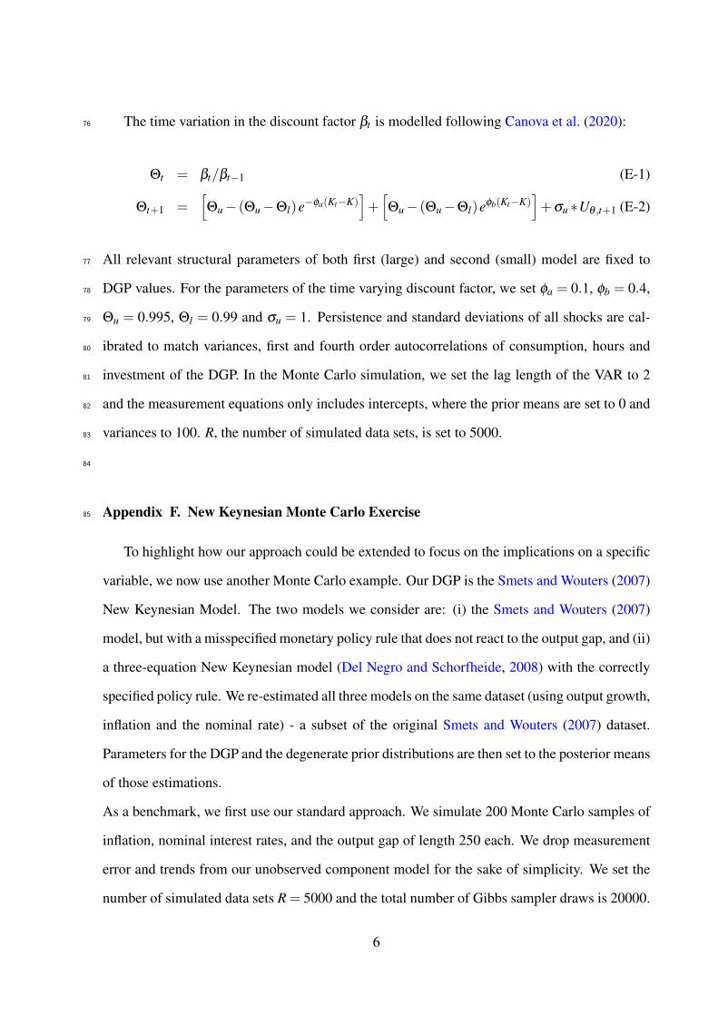
The time variation in the discount factor βt is modelled following Canova et al. (2020):76

Θt = βt/βt−1 (E-1)

Θt+1 =[Θu− (Θu−Θl)e−φa(Kt−K)

]+[Θu− (Θu−Θl)eφb(Kt−K)

]+σu ∗Uθ ,t+1 (E-2)

All relevant structural parameters of both first (large) and second (small) model are fixed to77

DGP values. For the parameters of the time varying discount factor, we set φa = 0.1, φb = 0.4,78

Θu = 0.995, Θl = 0.99 and σu = 1. Persistence and standard deviations of all shocks are cal-79

ibrated to match variances, first and fourth order autocorrelations of consumption, hours and80

investment of the DGP. In the Monte Carlo simulation, we set the lag length of the VAR to 281

and the measurement equations only includes intercepts, where the prior means are set to 0 and82

variances to 100. R, the number of simulated data sets, is set to 5000.83

84

Appendix F. New Keynesian Monte Carlo Exercise85

To highlight how our approach could be extended to focus on the implications on a specific

variable, we now use another Monte Carlo example. Our DGP is the Smets and Wouters (2007)

New Keynesian Model. The two models we consider are: (i) the Smets and Wouters (2007)

model, but with a misspecified monetary policy rule that does not react to the output gap, and (ii)

a three-equation New Keynesian model (Del Negro and Schorfheide, 2008) with the correctly

specified policy rule. We re-estimated all three models on the same dataset (using output growth,

inflation and the nominal rate) - a subset of the original Smets and Wouters (2007) dataset.

Parameters for the DGP and the degenerate prior distributions are then set to the posterior means

of those estimations.

As a benchmark, we first use our standard approach. We simulate 200 Monte Carlo samples of

inflation, nominal interest rates, and the output gap of length 250 each. We drop measurement

error and trends from our unobserved component model for the sake of simplicity. We set the

number of simulated data sets R = 5000 and the total number of Gibbs sampler draws is 20000.

6

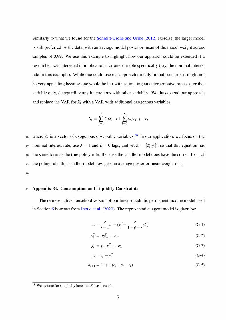
Similarly to what we found for the Schmitt-Grohe and Uribe (2012) exercise, the larger model

is still preferred by the data, with an average model posterior mean of the model weight across

samples of 0.99. We use this example to highlight how our approach could be extended if a

researcher was interested in implications for one variable specifically (say, the nominal interest

rate in this example). While one could use our approach directly in that scenario, it might not

be very appealing because one would be left with estimating an autoregressive process for that

variable only, disregarding any interactions with other variables. We thus extend our approach

and replace the VAR for Xt with a VAR with additional exogenous variables:

Xt =J

∑j=1

C jXt− j +L

∑l=0

MlZt−l + εt

where Zt is a vector of exogenous observable variables.28 In our application, we focus on the86

nominal interest rate, use J = 1 and L = 0 lags, and set Zt = [πt yt ]′, so that this equation has87

the same form as the true policy rule. Because the smaller model does have the correct form of88

the policy rule, this smaller model now gets an average posterior mean weight of 1.89

90

Appendix G. Consumption and Liquidity Constraints91

The representative household version of our linear-quadratic permanent income model used

in Section 5 borrows from Inoue et al. (2020). The representative agent model is given by:

ct =r

r+1at +(yP

t +r

1−ρ + ryT

t ) (G-1)

yTt = ρyT

t−1 + e1t (G-2)

yPt = γ + yP

t−1 + e2t (G-3)

yt = yTt + yP

t (G-4)

at+1 = (1+ r)(at + yt − ct) (G-5)

28 We assume for simplicity here that Zt has mean 0.

7

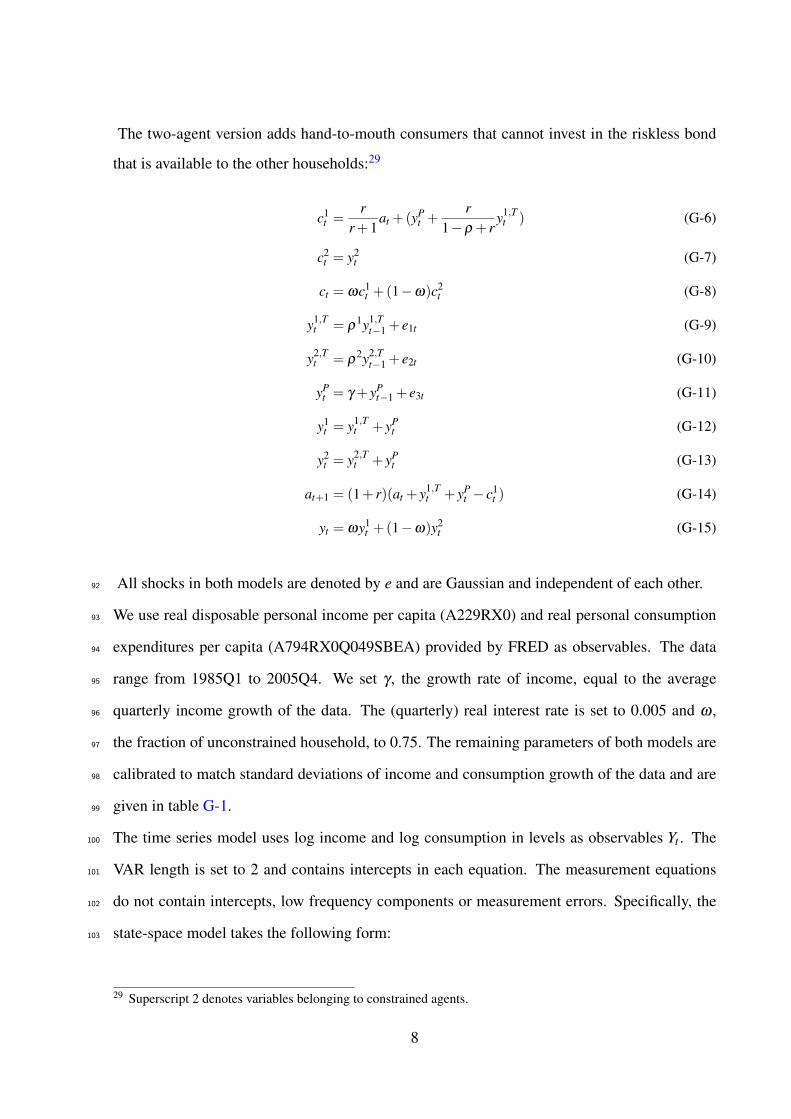
The two-agent version adds hand-to-mouth consumers that cannot invest in the riskless bond

that is available to the other households:29

c1t =

rr+1

at +(yPt +

r1−ρ + r

y1,Tt ) (G-6)

c2t = y2

t (G-7)

ct = ωc1t +(1−ω)c2

t (G-8)

y1,Tt = ρ

1y1,Tt−1 + e1t (G-9)

y2,Tt = ρ

2y2,Tt−1 + e2t (G-10)

yPt = γ + yP

t−1 + e3t (G-11)

y1t = y1,T

t + yPt (G-12)

y2t = y2,T

t + yPt (G-13)

at+1 = (1+ r)(at + y1,Tt + yP

t − c1t ) (G-14)

yt = ωy1t +(1−ω)y2

t (G-15)

All shocks in both models are denoted by e and are Gaussian and independent of each other.92

We use real disposable personal income per capita (A229RX0) and real personal consumption93

expenditures per capita (A794RX0Q049SBEA) provided by FRED as observables. The data94

range from 1985Q1 to 2005Q4. We set γ , the growth rate of income, equal to the average95

quarterly income growth of the data. The (quarterly) real interest rate is set to 0.005 and ω ,96

the fraction of unconstrained household, to 0.75. The remaining parameters of both models are97

calibrated to match standard deviations of income and consumption growth of the data and are98

given in table G-1.99

The time series model uses log income and log consumption in levels as observables Yt . The100

VAR length is set to 2 and contains intercepts in each equation. The measurement equations101

do not contain intercepts, low frequency components or measurement errors. Specifically, the102

state-space model takes the following form:103

29 Superscript 2 denotes variables belonging to constrained agents.

8

Yt = Xt

Xt = µ +C1Xt−1 +C2Xt−2 + εt , εtiid∼ N(0,Σε)

Mixture-priors are employed on µ,C1,C2,and Σε , whose prior hyperparameters are informed104

by VAR(2) estimates of simulated data.105

106

Table G-1: Calibration, Permanent Income Example

Parameter Value Target

r 0.0050 quarterly real interest rateγ 0.0051 average quarterly real income growth

Representative Agent Modelρ 0.2409 standard deviations of income and consumption growth

100×σe1 0.2995 standard deviations of income and consumption growth100×σe2 0.4636 standard deviations of income and consumption growth

Heterogeneous Agent Modelω 0.75 standard value in the literatureρ1 0.4998 standard deviations of income and consumption growthρ2 0.4999 standard deviations of income and consumption growth

100×σe1 0.4905 standard deviations of income and consumption growth100×σe2 0.0161 standard deviations of income and consumption growth100×σe3 0.4805 standard deviations of income and consumption growth

9

Appendix H. Debortoli and Galı (2018): RANK vs. TANK107

The Debortoli and Galı (2018) model used in Section 5 is described by the following set108

of equations, where we provide the description of the endogenous and exogenous variables in109

tables H-2 and H-3 and of the deep parameters in Table H-4. The calibration is presented in110

Table H-5, the priors for those parameters that are not set using information from the DSGE111

models can be found in Table H-6, whereas data used in estimation are listed in H-7.112

Appendix H.1. Parameter and Variable Definitions113

Table H-2: Endogenous Variables.

Variable Description

π inflation

y output gap

yn natural output

y output

rn natural interest rate

rr real interest rate

i nominal interest rate

n hours worked

h heterogeneity index

γ consumption gap

ν AR(1) monetary policy shock

a AR(1) technology shock

z AR(1) preference shock

rr,ann annualized real interest rate

iann annualized nominal interest rate

rn,ann annualized natural interest rate

πann annualized inflation rate

10

114

Table H-3: Innovations to Exogenous Shocks.

Variable Description

εν monetary policy shock

εa technology shock

εz cost-push shock

115

Table H-4: Deep Parameters.

Variable Description

β discount factor

λ fraction of constrained households

τ profit transfers

δ fraction illiquid to total assets

σ log utility

ϕ unitary Frisch elasticity

Ξ price adjustment cost

εp demand elasticity

φπ inflation feedback Taylor Rule

φy output feedback Taylor Rule

ρa autocorrelation exogenous monetary policy component

ρa autocorrelation exogenous technology process

ρa autocorrelation exogenous cost-push process

σν standard deviation, innovation to exogenous monetary policy component

σa standard deviation, innovation to exogenous technology process

σz standard deviation, innovation to exogenous cost-push process

11

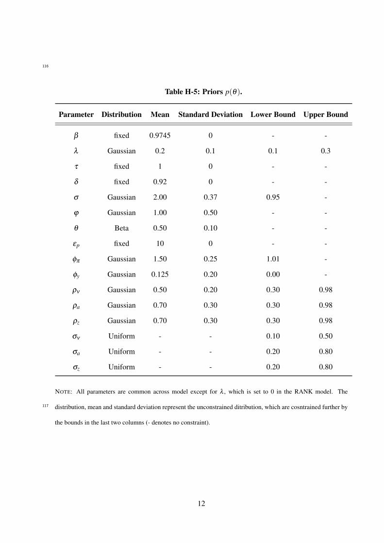
116

Table H-5: Priors p(θ).

Parameter Distribution Mean Standard Deviation Lower Bound Upper Bound

β fixed 0.9745 0 - -

λ Gaussian 0.2 0.1 0.1 0.3

τ fixed 1 0 - -

δ fixed 0.92 0 - -

σ Gaussian 2.00 0.37 0.95 -

ϕ Gaussian 1.00 0.50 - -

θ Beta 0.50 0.10 - -

εp fixed 10 0 - -

φπ Gaussian 1.50 0.25 1.01 -

φy Gaussian 0.125 0.20 0.00 -

ρν Gaussian 0.50 0.20 0.30 0.98

ρa Gaussian 0.70 0.30 0.30 0.98

ρz Gaussian 0.70 0.30 0.30 0.98

σν Uniform - - 0.10 0.50

σa Uniform - - 0.20 0.80

σz Uniform - - 0.20 0.80

NOTE: All parameters are common across model except for λ , which is set to 0 in the RANK model. The

distribution, mean and standard deviation represent the unconstrained ditribution, which are cosntrained further by

the bounds in the last two columns (- denotes no constraint).

117

12

Appendix H.2. Model Equations118

πt = β Etπt+1+κ yt + zt

where κ = ω (σ +ϕ) , ω =εp

ΞM pt

and M p =εp

εp−1

yt = yt+1−1

σ (1−Φ)

(it−πt+1− rn

t)

where Φ = λ(σ +ϕ) Ψ

1−λ γand Ψ =

(1−λ ) (1−δ (1− τ))(1−λ +

(M p

t −1)(1−λ δ (1− τ))

)2

it = πt−1 φπ + yt−1 φy +νt

rnt =−σ (1−ρa) ψ

nya at

rrt = it−πt+1

ynt = ψ

nya at , where ψ

nya =

1+ϕ

σ +ϕ

yt = yt− ynt

γt =−(σ +ϕ) Ψ yt

ht = Φ yt

νt = ρa νt−1− ενt

at = ρa at−1 + εat

zt = ρa zt−1 + εzt

yt = at +nt

iannt = 4it , rr,ann

t = 4rrt , rn,ann

t = 4rnt , π

annt = 4πt

13

Appendix H.3. Priors for RANK/TANK Application119

Table H-6 lists the priors used in our empirical application for those parameters that are not120

set using information from the DSGE models. The mean of an inverse gamma distribution is121

determined by a scale parameter scale and a shape parameter shape such that its mean (if it122

exists) is equal to scaleshape−1 and the variance (if it exists) is given by scale2

(shape−1)2(shape−2) .

Table H-6: Additional Priors.

Parameter Distribution Mean Information on Standard Deviation

µ Gaussian 0 1 for free elements, 0 elseΣu,i Inverse Gamma ∀i 0.22 ∞ (scale parameter of 2)Σw,i Inverse Gamma ∀i 0.52 for GDP, 0.22 else shape parameter is set to T/2X0 Gaussian 0 10µz Gaussian 0.25 for GDP, 0 else 0.50 for GDP, 0 else

123

124

125

Appendix H.4. Data for RANK/TANK Application126

In Table H-7 we report the data used in the RANK/TANK application.127

Table H-7: Data Information for RANK/TANK Application.

Variable Sample Transformation

GDP 1970:Q1-2019:Q4 seasonally adjusted, per-capita, then logGDI 1970:Q1-2019:Q4 seasonally adjusted, per-capita, then logCPI 1970:Q1-2019:Q4 seasonally adjusted, logPCE price index 1970:Q1-2019:Q4 seasonally adjusted, logThree month treasury bill rate 1970:Q1-2019:Q4 average over the quarterFederal Funds rate 1970:Q1-2019:Q4 average over the quarterWu-Xia shadow rate 1990:Q1-2019:Q4 average over the quarter

NOTE: The data is from the St. Louis Fed’s FRED database, except for the Wu-Xia shadow rate, which is down-

loaded from https://www.atlantafed.org/cqer/research/wu-xia-shadow-federal-funds-rate.128

129

130

14

Appendix H.5. Further Results for the RANK/TANK Application131

To highlight how our approach can be used to estimate a cyclical component informed by132

economic theories, Figure H-2 plots the median and 5th as well as 95th percentiles for the cycli-133

cal component of real GDP (i.e. the posterior estimates of one element of Xt) in the left panel134

(NBER recessions are depicted using gray bars). We can see that the estimated cyclical compo-135

nent tends to decline during recessions, as predicted by our theories.136

137

1960 1970 1980 1990 2000 2010 2020-15

-10

-5

0

5

10

15

Figure H-2: Estimated Cyclical Component for (Log) Per-Capita Real GDP.

To understand what helps us discriminate between these two models, it is useful to dig138

deeper into the structure of the models. It turns out that in the setup of Debortoli and Galı139

(2018), heterogeneity only appears in the IS equation (i.e. the consumption Euler equation).140

Both the RANK and the TANK model share the same IS equation:141

yt = Etyt+1−1

σ (1−Φ(λ ))(it−Etπt+1− rn

t ) , (H-1)

where yt is the output gap, πt is inflation, it is the nominal interest rate, and rnt is the natural142

real rate in the model (all measured in deviations from steady state). The key object is Φ(λ ),143

which is a composite parameter that depends, among other things, on the fraction of restricted144

households λ .145

15

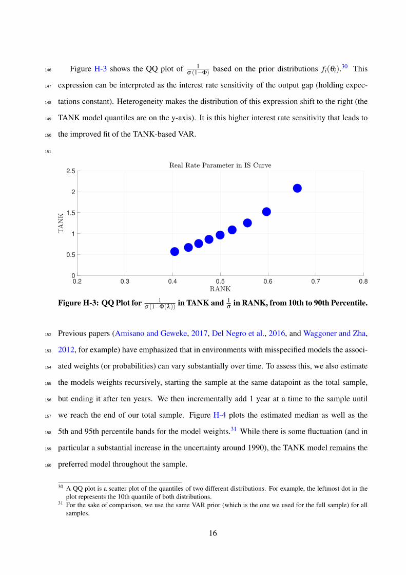
Figure H-3 shows the QQ plot of 1σ (1−Φ) based on the prior distributions fi(θi).30 This146

expression can be interpreted as the interest rate sensitivity of the output gap (holding expec-147

tations constant). Heterogeneity makes the distribution of this expression shift to the right (the148

TANK model quantiles are on the y-axis). It is this higher interest rate sensitivity that leads to149

the improved fit of the TANK-based VAR.150

151

0.2 0.3 0.4 0.5 0.6 0.7 0.80

0.5

1

1.5

2

2.5

Figure H-3: QQ Plot for 1σ (1−Φ(λ )) in TANK and 1

σin RANK, from 10th to 90th Percentile.

Previous papers (Amisano and Geweke, 2017, Del Negro et al., 2016, and Waggoner and Zha,152

2012, for example) have emphasized that in environments with misspecified models the associ-153

ated weights (or probabilities) can vary substantially over time. To assess this, we also estimate154

the models weights recursively, starting the sample at the same datapoint as the total sample,155

but ending it after ten years. We then incrementally add 1 year at a time to the sample until156

we reach the end of our total sample. Figure H-4 plots the estimated median as well as the157

5th and 95th percentile bands for the model weights.31 While there is some fluctuation (and in158

particular a substantial increase in the uncertainty around 1990), the TANK model remains the159

preferred model throughout the sample.160

30 A QQ plot is a scatter plot of the quantiles of two different distributions. For example, the leftmost dot in theplot represents the 10th quantile of both distributions.

31 For the sake of comparison, we use the same VAR prior (which is the one we used for the full sample) for allsamples.

16

1970 1975 1980 1985 1990 1995 2000 2005 2010 2015 20200.5

0.6

0.7

0.8

0.9

1

Figure H-4: Recursive Model Weights (5th, 50th, and 95th Percentiles).

Our approach is different from aforementioned pooling approaches such as Amisano and Geweke161

(2017) or Del Negro et al. (2016) when those approaches directly pool dynamic equilibrium162

models. In such pooling approaches, the one-step ahead forecast density has to be a weighted163

average of the forecast densities from the individual equilibrium models. Our approach instead164

delivers a forecast density that generally is not a weighted average of the densities coming di-165

rectly from the equilibrium models, and thus has an advantage if the individual equilibrium166

models are severely misspecified.167

Appendix H.6. Forecasting Performance in the RANK/TANK Application168

We next study the forecasting performance of our approach. To get a sense of how well169

our model performs, we study the relative root mean squared error (RMSE) for our six observ-170

ables relative to a benchmark forecasting model. We recursively add data to both models and171

re-estimate every year (the recursive estimation of our model also delivered Figure H-4). As172

this benchmark forecasting model we choose an ARIMA(p,d,q) model where p denotes the173

AR lag length, q denotes the MA lag length, and d denotes the order of integration. We select174

the model specification using the Akaike information criterion (AIC) to maximize forecasting175

performance. For each recursive sample, we first conduct ADF tests to determine the order of176

integration. The test specification includes a constant and the lag length is set based on the AIC.177

Then, we determine p and q also based on the AIC where the maximum p and q are set to 8.178

Table H-8 shows the relative RMSE, where a number larger than 1 implies a better performance179

17

of the ARIMA model. Two findings stand out: (i) similar to Del Negro and Schorfheide (2004),180

our approach does better at medium horizons compared to very short horizons, and (ii) our ap-181

proach performs better for the nominal variables in our sample. In order to improve forecasting182

performance for GDP and GDI, we could modify the law of motion for zt to allow for richer183

trend dynamics (see for example Canova, 2014).184

Table H-8: Relative RMSE (of VAR/ARIMA) by Forecast Horizon h (in Quarters).

h=1 h=2 h=3 h=4 h=5 h=6 h=7 h=8

GDP 1.4 1.2 1.2 1.1 1.1 1.1 1.2 1.2GDI 1.2 1.1 1.1 1.1 1.1 1.1 1.2 1.2CPI Inflation 1.0 0.9 0.8 0.9 0.9 0.9 0.8 1.0PCE Inflation 1.0 1.0 1.0 1.0 1.0 0.9 0.9 1.03-Month Treasury Bill 1.2 0.8 0.8 0.9 1.0 1.1 1.1 1.0Federal Funds Rate 1.2 1.1 0.8 0.8 0.9 0.9 0.9 0.9

Appendix I. More on the Relationship Between Our Approach and Standard Bayesian185

Model Probabilities186

It is well known that standard Bayesian model probabilities include an overfitting penalty, as187

is evident, for example, from the form of the well-known Bayesian Information Criterion, which188

approximates the Bayes factor in one particular situation. In standard marginal likelihood com-189

parisons, overfitting gets penalized because having more parameters can lead to substantially190

worse fit for some parameter values, which a marginal likelihood comparison will acknowledge191

since it is the integral of the product of prior and likelihood over the entire parameter space.192

In our approach something similar can happen, although the effects are likely muted: Our ap-193

proach builds on marginal likelihoods for VARs with different priors, but the same number of194

parameters. Priors for the VARs associated with theories (or DSGE models) with more param-195

eters might put more prior mass on regions of the parameter space that do not fit the data as196

well because these VAR priors are informed by the priors for the DSGE models. So parameter197

combinations that do not fit the data as well do still enter the marginal likelihood comparison198

for the VAR structure via the VAR priors.199

18