Embed Size (px)
Citation preview

Economic Growth and
The Public Sector
A selection of papers and abstracts presented at the
5th Global Conference
Forum for Economists International
Amsterdam, May 29-June 1, 2015
Edited by
M. Peter van der Hoek
Erasmus University (Em.), Rotterdam, Netherlands
Academy of Economic Studies, Doctoral School of Finance & Banking,
Bucharest, Romania
and
Ternopil National Economic University, Ternopil, Ukraine
Forum for Economists International
Papendrecht, Netherlands
EI

ii
© Forum for Economists International 2015
All rights reserved. No part of this publication may be reproduced, stored in a
retrieval system or transmitted in any form or by any means, electronic, me-
chanical or photocopying, recording, or otherwise without the prior permission
of the publisher.
Published by
Forum for Economists International
PO Box 137
Papendrecht
Netherlands
Email: [email protected]
ISBN 978-90-817873-7-6

iii
Contents
List of contributors iv
PAPERS
1. Dynamic performance of state tax revenues: growth and 1
reliability of major state taxes
John Mikesell
2. Ethical considerations in public procurement: the case of 22
the South African public service: evidence from panel data
David Fourie
3. Infrastructure and economic growth in Sub-Saharan Africa 46
Odongo Kodongo and Kalu Ojah
4. Public debt dynamics in Kenya 58
Conrado Garcia, Armando Morales and Lydia Ndirangu
5. Household income inequality in Poland from 2005 to 2013 – a 73
decomposition of the Gini coefficient by income source
Patrycja Graca-Gelert
6. Analysis of the relationship between profitability and dividend 94
policy of banks on the Ghana stock exchange
John Kwaku Mensah Mawutor and Embele Kemebradikemor
ABSTRACTS
7. Corruption, Regime Type, and Economic Efficiency: A 110
Cross-Country Study
Ilan Alon, Shaomin Li and Jun Wu
8. The Analysis of Split Graphs in Social Networks Based on the 112
k-cardinality Assignment Problem
Ivan Belik

iv
9. Optimal tax policy in a small open economy with credit constraints. 113
The theoretical model plus calibration and conclusions for Poland
Michał Konopczyński
10. Relationship between Environmental Degradation and Economic 118
Development: A Panel Data Analysis
Selin Özokcu and Özlem Özdemir Yilmaz
11. Explaining Immigrant Health Service Utilization: A Modified 119
Theoretical Framework
Philip Q. Yang and Shann Hwa Hwang

v
Contributors
Ilan Alon, University of Agder, School of Business and Law, Kristiansand,
Norway
Ivan Belik, Norwegian School of Economics, Bergen, Norway
David Fourie, School of Public Management and Administration, University
of Pretoria
Conrado Garcia, USAID/Kenya, Nairobi, Kenya
Patrycja Graca-Gelert, Warsaw School of Economics, Warsaw, Poland
Shann Hwa Hwang, Texas Woman's University, Denton, TX, USA
Embele Kemebradikemor, Wisconsin International University College, Ac-
cra, Ghana
Odongo Kodongo, Wits Business School, University of the Witwatersrand,
Johannesburg, South Africa
Michał Konopczyński, Poznań University of Economics, Poznań, Poland
Shaomin Li, Old Dominion University, Norfolk, VA, USA
John Kwaku Mensah Mawutor, University of Professional Studies, Accra,
Ghana
John L. Mikesell, Indiana University, Bloomington, IN, USA

vi
Armando Morales, International Monetary Fund, Nairobi, Kenya
Lydia Ndirangu, Central Bank of Kenya and Kenya School of Monetary
Studies, Nairobi, Kenya
Kalu Ojah, Wits Business School, University of the Witwatersrand, Johan-
nesburg, South Africa
Özlem Özdemir Yilmaz, Middle East Technical University, Ankara, Turkey
Selin Özokcu, Middle East Technical University, Ankara, Turkey
Jun Wu, Savannah State University, Savannah, GA, USA
Philip Q. Yang, Texas Woman's University, Denton, TX, USA
1
1 DYNAMIC PERFORMANCE OF STATE
TAX REVENUES: GROWTH AND RELIABILITY
OF MAJOR STATE TAXES
John L. Mikesell
Chancellor’s Professor
School of Public and Environmental Affairs
Indiana University
Bloomington, Indiana
Abstract
State tax reliability is critical for provision of many services important to society. Be-
cause states are significantly constrained in their capacity to run operating deficits, service
maintenance depends critically on state tax performance. Both revenue growth and revenue
reliability matter. Slow revenue growth can limit the capacity of the state to respond to grow-ing demand for services. Unreliable revenue can force states to make radical changes in ser-
vice delivery, sometimes even after legislatures have adopted spending programs for the year.
This paper examines growth and reliability of major American state taxes over the period
from 1970 to 2013. It examines the extent to which the growth and reliability attributes may
be inconsistent, a particular concern in this period that includes the Great Recession. Evi-
dence shows that, although the total tax growth rate is generally robust, around 6% for most
states, individual taxes show considerable variation in rates across both taxes and states.
However, there is more variation in volatility than in growth rates of the taxes. Growth and
stability do not appear to be incompatible objectives and diversification appears not to matter
for either growth or reliability.
1.1. Dynamic Performance of State Tax Revenues: Growth and Stability
of Major State Taxes
The American fiscal system traditionally presumes that states will finance
the services that they provide from their own tax systems. States cannot expect
the national government to provide general state support to or to mitigate fis-
cal problems a state might encounter. Federal transfers (30% of total state
general revenue in fiscal 2013) are conditional, intended for support of ser-
vices of particular national interest, e.g., Medicaid or interstate highways, and
are not freely available for purposes deemed most important by state lawmak-
ers. (Governments Division, U. S. Bureau of Census) State revenue systems
are legally independent of those of the national government, their administra-
tion is a decentralized state responsibility, and there is no general transfer
structure for distributing nationally collected tax revenue to states. (Duncan
and McLure, 1997) Because states have limited capacity to finance operating
deficits and have primary responsibility for provision of services vital for a
civilized society, including education, public safety, transportation, elections,
etc., the ability of state tax systems to raise adequate revenue is crucial. State

Mikesell
2
tax system failures would spell catastrophe for the operation of the entire fiscal
system so their performance as revenue producer merits substantial attention
and concern.
This article examines the dynamic portfolio changes in state tax systems,
tax system growth and reliability in recent years, the extent to which the reve-
nue portfolio structure may influence dynamic performance, and their respon-
siveness in national economic recession.
2. The Shape of State Tax Structures
States enjoy almost complete flexibility in terms of what taxes they may
levy, at least in terms of federal Constitutional constraints. As Wildasin (2007,
651) observes, “Indistinct though its boundaries may be, the residual taxing
authority of the states granted by the Constitution evidently accommodates
non-trivial diversity in state and local revenue structures.” States choose their
own tax systems and most of the more productive, broad-based state taxes
were adopted either in the 1930s or the 1960s, the first decade being an era of
great economic challenge and the second being one of expanding state respon-
sibilities. (Mikesell, 2015, 44) By 1970 the current state tax systems were
largely in place. Only five states do not already levy a general sales tax and
only seven states levy no individual income tax (two more apply only a very
narrow income tax), so there is little room for major realignments for addi-
tional revenue –the productive taxes are already in place. States not levying
one of the major tax bases are so adverse to the omitted tax that new adoptions
are unlikely.
Adoptions since the 1970s have generally been in regard to taxes with
limited revenue potential, like excises on casino gaming and low-productivity
gross receipts taxes.1 Although states use the freedom given by the federal sys-
tem to structure their tax systems as they choose and although they do levy a
wide variety of selective sales, license, documentary, severance, and other tax-
es, in virtually all instances, the most productive taxes for states are the indi-
vidual income tax and the general sales tax. Exceptions are Alaska (corporate
net income tax), North Dakota (severance tax), and Wyoming (severance tax).
In general, productive alternatives are not likely to be added to the current
state tax mix.
Nevertheless, within the tax portfolio, the mix has changed. The structural
pattern of state tax systems can be seen by analysis using two standard
measures of diversification and concentration, a Herfindahl-Hirschman index-
based diversification ratio (DIV) and the tax concentration ratio (C). While the
1. Ohio, Pennsylvania, and Rhode Island adopted broad individual income taxes in 1971 and
New Jersey adopted that tax in 1976.

Dynamic performance of state tax revenues 3
measures were initially developed for investigation of the concentration of
firms in an industry, they also serve as a basis for considering the concentra-
tion of reliance on a limited number of taxes in a state tax structure.
Diversification
The diversification ratio is calculated from the HHI :
where S equals the share of total tax revenue from each of the n taxes levied
by the government. The raw HHI measures concentration rather than diversity
and the range of HHI ranges from a minimum that depends on the number of
taxes for which the measure is calculated to a maximum of 1.0 (all revenue
from a single tax).2 The HHI is converted to a normalized indicator of diversi-
fication (DIV) according to the formula:
DIV = (HHI – 1) / minimum HHI
For any given state tax portfolio, the calculated diversification ratio de-
pends on how fine the categorization of taxes is, but for any given categoriza-
tion, the higher the ratio, the greater the diversification (to a maximum of
1.0).3 Ratios do differ according to how fine the categorization used for calcu-
lation is but the ratios are closely correlated.
Concentration
C equals the share of total tax revenue that is produced by the largest tax
sources, for instance, the share of total tax revenue raised from the individual
income and general sales taxes combined, the two most productive state taxes
since the middle of the last century. If a state levied only individual income
and general sales taxes, then C would equal 1.0; if it levied neither, C would
equal 0.0. Unlike DIV, the top two concentration ratio used here is independ-
ent of the breakdown of taxes in the portfolio, so coefficients on this variable
in regression analysis can be meaningfully interpreted.
2. The tax portfolio may be divided at various degrees of disaggregation, i.e., including a total
selective excise category versus dividing excises into motor fuel, alcoholic beverage, parimu-
tuels, etc., and the degree of disaggregation will determine the minimum for the HHI. The
calculated HHIs across states will vary according to the disaggregation.
3. The seventeen categories used in this calculation are the following: property tax, general
sales tax, alcoholic beverage tax, amusement tax, insurance premium tax, motor fuels tax,
parimutuels tax, public utility tax, tobacco tax, other selective excises, total license taxes, in-
dividual income tax, corporate net income tax, death and gift tax, documentary and stock transfer tax, severance tax, and taxes not elsewhere classified.

Mikesell
4
Changing Structural Pattern
Figure 1 traces DIV and C over the period from 1970 through 2013, forty
years with a virtually constant set of major taxes in each state tax structure.4
The profile is clear: state tax revenues have become less diversified, as the
DIV went from 0.841 in 1970 to 0.7567 in 2013, a 10% decline in diversity.
However, DIV does not give the full picture. The two-tax (income and general
sales) concentration ratio went from 0.464 in 1970 to 0.6153 in 2013, a 33%
increase in concentration. State tax structures are less diversified and much
more reliant on two major taxes than they were in 1970 – they are moving to-
ward generating two-thirds of their tax revenue from only the two taxes.
There are some reasons behind this reduced diversification/increased two-
tax concentration. Excises and license revenues have not kept up because
many are levied on unit bases that do not pick up inflation and state lawmakers
have been reluctant to increase statutory tax rates. Corporate income tax reve-
nues have not kept up because of state policies that seek to accommodate
business activity by reducing burden on in-state corporate activity, e.g., reduc-
ing property and payroll components of profit apportionment formulas. In ad-
dition, there has been a great movement away from organizing the business as
a traditional corporation toward organizing the business as a pass-through enti-
ty not subject to business-level taxation. Real property taxes have become po-
litical anathema and states have moved away from use of the source. Not all
states have severance tax prospects and some of those that do have limited po-
litical will to make heavy use of the source. The sum of these influences cre-
ates the concentration of tax structures on the individual income and general
sales taxes, taxes that do respond to inflation and economic growth, even as
4. The annual data come from U. S. Bureau of Census, Governments Division.

Dynamic performance of state tax revenues 5
lawmakers are reluctant to raise statutory rates. Barring some dramatic exter-
nal change, the two-tax concentration is not likely to decline and tax diversifi-
cation is not likely to increase.5
3. State Taxes and the National Economy
Collections from four taxes – individual income, general sales, corporate
net income, and motor fuels – constitute somewhat more than three-quarters of
total state tax revenue. All are susceptible to revenue fluctuations with changes
in the national economy. While reductions in tax collections when the national
economy is heading to recession may help stabilize the economy, those reduc-
tions can create difficult fiscal problems for state governments. It is useful to
understand how state tax collections are impacted by national economic
change, particularly taking into account behavior through the recent Great Re-
cession. Given that the national economy has experienced two rather severe
recessions in the first two decades of the twenty-first century, it is particularly
interesting to see what the state tax impact has been.
Tax Collections and GDP Change
This section will examine how real change in revenue from these taxes is
related to real change in national gross domestic product. Although state
budgets are not prepared in real terms, the analysis here works with price-
adjusted GDP and tax revenues because movements in real GDP are often as-
sociated with the national economic cycle and this adjustment provides focus
on that influence. Each tax appears to be related to economic change, but the
extent of the relationship is not the same for all taxes.
Figures 2-5 trace out the path of percentage change in real GDP and the
four major state taxes from 1970 through 2013. Over that period, there were
six full national recessions: IV:1973–I:1975, I:1980–III: 1980, III:1981–
IV:1982, III:1990–I:1991, I:2001–IV:2001, and IV:2007–II:2009. Considera-
ble reductions in real GDP are apparent in the figures for each of these reces-
sions, with percentage change being negative in 1974, 1982, and 2008-2010.
The path of annual change in real GDP is never smooth in the period, with
considerable differences in change rates from one year to the next. The signi-
fication exception occurs during the long expansion from 1991 to 2000 when
real growth never fell below 2.5% and was usually somewhat higher.
The figures show annual change in real state revenue from the four taxes
to usually follow the profile of annual change in real GDP, although the im-
pact on revenue change often lags change in real GDP.
5. Even with this considerable concentration in state tax systems, state structures are more
diversified than those of local (heavily property tax reliant) and federal (heavily reliant on the income base) governments.

Mikesell
6
(i) General Sales Tax
Percentage change in real general sales tax revenue is zero or negative with
the recessions of 1975 (somewhat lagging the change in GDP), 1981, 1991,
2001 (again lagging the change in GDP), and 2009, as shown in Figure 2. The
impact is greatest in the last recession, with percentage change in 2009 equal-
ing -6.3%. That impact is far greater than in any of the earlier recessions
(change was negative in 1981 and 2003). The average percentage change in
general sales tax revenue was 4.93% or 5.33% for average absolute percentage
change. The correlation between percentage change in real GDP and real gen-
eral sales tax revenue is 0.6678.

Dynamic performance of state tax revenues 7
(ii) Individual Income Tax
Percentage change in individual income tax collections is approximately zero
or negative in 1991, 2002 – 2003, and 2009 – 2010, as shown in Figure 3. The
negative change was 12% in both 2002 and 2009, although real GDP growth
was negative only in the latter year. That many of these zero or negative years
coincide with similar results for general sales taxes, the two most significant
state taxes, indicates a considerable problem for state finances. The average
percentage change in individual income tax revenue was 6.79% or 7.95% in
average absolute percentage change. The correlation between percentage
change in real GDP and real individual income tax revenue is 0.5041.
(iii) Corporate Net Income Tax
State corporate net income tax collections were subject to dramatic swings in
the 1970 – 2013 period, with two years showing percentage increases in ex-
cess of 20% (and many with increases above 10%) and two years with de-
creases greater than 20%, as shown in Figure 4. Collection changes were more
extreme than changes in GDP and collection declines were particularly great
in the last two national recession periods. Average percentage change for real
corporate net income tax revenue was 4.18, 8.53% in average absolute change.
There are particularly large percentage changes in recession periods and large
increases in the early 1970s and in the mid-2000s. The correlation between
percentage change in real GDP and real corporate net income tax revenue was
0.4892.
(iv) MotorFuels Tax
Motor fuel tax collections do not exhibit swings in annual change that are as
dramatic as some other taxes. In many years, their change is considerably less
than seen for real GDP. Annual change in collections is negative in a few

Mikesell
8
years, usually around a recession period, but negative change is never as great
as 5%, as shown in Figure 5. The average percentage change over the period is
only 2.12% or 2.93% for average absolute change, averages that are consider-
ably less than for the other three taxes. The correlation between percentage
change in real GDP and real motor fuel tax was low and negative, -0.172. Be-
havior of the motor fuel tax is considerably different from that of the other ma-
jor taxes.
(v) Total Taxes
Figure 6 presents the relationship between percentage change in real GDP and
real total tax collections for the states. There are substantial fluctuations in real
collections, with the percentage change being larger than a negative 5%
around the last two recessions. The percentage change was near-zero in earlier
recessions of the 1970s, 1980s, and 1990s, but never as dramatic as the 2002
and 2009 experience. The average percentage change was 4.32% or 4.90% in
average absolute terms. The correlation between percentage change in real
GDP and real total tax collections over the 1970 – 2013 period was 0.643, a
higher correlation than for any of the big four taxes except for the general
sales tax.

Dynamic performance of state tax revenues 9
4. Cyclical Sensitivity of the Major Taxes: Cyclical Swing Evidence
Changes in state tax collections that follow the national business cycle
may make macroeconomic stabilization more difficult for the economy as a
whole and will challenge the ability of state governments to maintain im-
portant services to the public. The cyclical sensitivity of tax revenue can be
examined with the cyclical swing index, a direct measure of the ability of tax
sources to be insulated from the impact of the national economic cycle.
Friedenberg and Bretzfelder (1980, 27) define the cyclical swing measure to
equal the “difference between (1) the percentage-point difference between the
mean quarterly percentage change in the expansion(s) and the mean quarterly
percent change in the whole cycle)s) and (2) the percentage-point difference
between the mean quarterly percent change in the recession(s) and the mean
quarterly percent change in the whole cycle(s).” Because economic cycles are
frequently short and do not match up with either complete fiscal or calendar
years, it is important to examine this cyclical sensitivity with quarterly data, as
the cyclical swing does.
The cyclical swing (CS) equals the following:
CS = [PCHe – PCHc] – [PCHr – PCHc]
where PCH = mean quarterly change and subscripts e, r, and c designate
change in expansion, recession, and the full period examined. The measure
adjusts for trend by working with differences in comparable growth rates and
eliminates seasonal variation by use of seasonally adjusted collections data.
The index shows whether growth in revenue from a particular tax drops sub-
stantially during a recession or whether the growth pattern remains generally
constant through expansion and recession. A high positive CS means substan-

Mikesell
10
tially greater growth during expansion than during contraction. By using quar-
terly data and by linking the analysis directly to business cycle dates, the
measure directly captures a major concern for state governments. The cycle is
based on National Bureau of Economic Research dating.
Data for this analysis come from quarterly collections data available from
the Governments Division, Bureau of the Census. (U. S. Bureau of Census,
Governments Division) The raw data for the first quarter 2001 through the
second quarter of 2009 (two full recessions and one full expansion) are sea-
sonally adjusted and the index was calculated for both current and constant
dollar changes.
The cyclical swing results appear in Table 1. The evidence is that corpo-
rate net income tax collections are most dramatically cyclically unstable. The
index is 9.015 for current prices and 8.573 for constant prices, a great differ-
ence in behavior between expansion and recession. That index is more than
double that of any other tax examined here, evidence of great sensitivity of
corporate profits to the economic cycle. The next most cyclically sensitive tax
is that on individual income, with a cyclical swing of 4.210 in current prices
and 3.680 in constant prices, followed by general sales taxes, with a cyclical
swing of 2.783 in current prices and 2.508 in constant prices. This shows a
considerable difference in behavior between expansion and recession phases.
The index for motor fuel tax collections is substantially lower than for the oth-
er taxes, only 0.9135 for current prices and 0.269 for constant prices. There is
little difference in annual revenue change between recession and expansion for
this tax, meaning that this tax is relatively stable through the economic cycle.
The tax may have growth issues created by its rate being usually applied to the
number of units purchased, not the value of the purchase, but it does not ap-
pear to have the cyclical sensitivity of the other major tax sources.
Table 1. Major State Taxes -- Cyclical Swing Indicators,
2001:I to 2009:II
Cyclical Swing
(Current $)
Cyclical Swing
(Constant $)
Total Taxes 3.260 2.892
General Sales Taxes 2.7838 2.508
Motor Fuels Taxes .9135 0.269
Individual Income Taxes 4.210 3.680
Corporate Net Income Taxes 9.015 8.573
5. Tax Revenue Growth and Reliability for States
State tax reliability is critical for provision of many services important to
society. Because states are significantly constrained in their capacity to run

Dynamic performance of state tax revenues 11
operating deficits, service maintenance depends critically on state tax perfor-
mance. Dynamic problems with tax revenue will translate directly into service
delivery issues and intended expenditure programs will have to be curtailed,
sometimes even during budget execution when collections fall short of
amounts forecast when the budget was adopted. Both revenue growth – the
pattern of collections over several years -- and revenue variability matter to
provision of state government services. Slow revenue growth can limit the ca-
pacity of the state to respond to growing demand for services and revenue in-
stability can force states to make radical changes in service delivery. Dye and
McGuire (1991, 55) sum up the problem: “[The growth rate and its variability]
are of great importance to policymakers who must devise revenue systems that
can both support expenditure programs over the long run and provide stable
steams of revenue even as the underlying economy varies with the business
cycle.”
This section examines growth and stability of four major state taxes over
the period from 1970 to 2013. The taxes together constituted 76% of total state
tax revenue in 2013: individual income, 36.6%; general sales and gross re-
ceipts, 30.1%; corporate net income, 5.3%; and motor fuel, 4.7%. These are
the only taxes yielding as much as 3% of the total, although some taxes do
yield more in the revenue portfolio of a particular state.
The dynamic behavior of individual state tax systems will be examined
through three indicators.
(i) Growth rate
The long-term growth rate indicates the ceiling for state service provision un-
der a balanced budget constraint, either imposed legally or from economic re-
ality. In this analysis, the rate is estimated from the equation
Ln R = a + b t
where R = tax revenue, either from all state taxes or from a particular state tax;
b = the long-term growth rate; and t = the fiscal year of observation less 1969.
(2) Volatility
Revenue variability indicates the extent to which tax collections diverge from
the long-term growth rate. Even if the tax base is growing substantially over
the long term, large fluctuations around that growth path can significantly dis-
rupt state finances. Such fluctuations can require troublesome adjustments in
state fiscal programs to maintain a sustainable financial profile. The Williams-
Anderson-Froehle-Lamb z (Williams et al., 1973) coefficient measures volatil-
ity in terms of divergence from the growth rate of the tax base. Operationally
it equals the inverse of the standard error of the equation used to calculate the
growth rate:

Mikesell
12
where SlnR = the standard error of the growth rate equation and
A higher z value means that yield growth is more volatile.
(3) Stability
The coefficient of variation (CV) of the tax base measures the dispersion (or
spread) of tax revenue over several years relative to average tax revenue. The
higher the CV, the greater the variation in the annual value of tax revenue and,
hence, the more unstable is the tax.
Experience of state tax structures are examined here for the 1970 – 2013
period. Data are taken from the Governments Division, U. S. Bureau of Cen-
sus and the Bureau of Economic Analysis of the U. S. Department of Com-
merce.
5.1 Growth
The growth rates for all state taxes and from the four largest revenue con-
tributors appear in Table 2. The average across all states for total taxes is a
growth rate of 6.6% in current dollars (3.3% in real terms). The average cur-
rent dollar growth rate for the ten states with the slowest growth is 5.7%, com-
pared with an average rate of 7.6% for the ten states with the fastest growth.
The growth rate in Nevada, 9.3% (or 5.9% in real terms), is an extreme outlier,
being 1.5 percentage points higher than the rate for the next state. The states
with fastest growth include two states with no individual income tax and one
state with no general sales tax; the states with slowest growth all levy both
those taxes. There is no clearly discernable geographic pattern to slow versus
rapid growth of total tax revenue.
There are differences in growth for the major taxes.
(i) Individual income tax revenue growth averaged 8.1% (4.7% in real
terms). There is a considerable difference in state growth rates. The aver-
age current dollar rate for the ten slowest growing taxes was 6.4%, while
the average for the ten fastest growing was 10.3%. There is no apparent
regional pattern to the differences in growth rates.
(ii) General sales tax revenue growth averaged 6.6% (3.2% in real terms),
considerably slower than the rate for individual income taxes. The aver-
age rate in the ten states with slowest sales tax growth was 5.4%, com-
pared with 8.1% for the states with fastest growth. The three states with

Dynamic performance of state tax revenues 13
highest general sales tax growth (Nevada, Texas, and Florida) levy no in-
dividual income tax. All the ten slowest growth general sales tax states al-
so levy an individual income tax.
(iii) Corporate net income tax revenue growth averaged 5.7% (2.5% in real
terms), a rate lower than for both general sales and individual income tax-
es. There was, however, considerable variation across states in this rate,
from below 4% in eight states (Ohio Connecticut, South Carolina, Rhode
Island, Pennsylvania, Michigan, Louisiana, and Hawaii) to over 8% in
five states (New Hampshire, Alaska, West Virginia, Indiana, and South
Dakota). Many states have manipulated their corporate income tax struc-
tures in an effort to encourage economic development, making the rela-
tively low growth rate unsurprising.
(iv) Motor fuel tax revenue grew by only 4.5% (1.3% in real terms), the low-
est rate for the four major taxes. Only four states (Utah, Texas, Arizona,
and Nevada) showed growth of 6% or more and Alaska, New York, and
New Jersey had growth rates below 3%. The taxes are levied on a unit ba-
sis, very few states have rates with adjustment mechanisms that pick up
the impact of inflation, and there are political difficulties associated with
attempting to increase the tax rate by legislative action. That combines
with the secular increase in motor vehicle fuel economy to produce the
relatively slow revenue growth, creating a difficult problem for mainte-
nance and construction of highway infrastructure.
Table 2. Growth Rates for Individual Income, General Sales, Corporate Income,
and Motor Fuels Taxes, 1970 - 2013
State Total
Tax,
Nomi-
nal
Total
Tax,
Real
Indi-
vidual
In-
come,
Nomi-
nal
Indi-
vidual
In-
come,
Real
Gen-
eral
Sales,
Nomi-
nal
Gen-
eral
Sales,
Real
Cor-
porate
Net
In-
come,
Nomi-
nal
Cor-
porate
Net
In-
come,
Real
Motor
Fuels,
Nomi-
nal
Motor
Fuels,
Real
AK 6.9% 3.5% No tax No tax No tax No tax 9.1% 5.7% 2.2% 1.2%
AL 6.0% 2.6% 8.0% 4.6% 5.4% 2.0% 5.7% 2.3% 3.9% 0.6%
AR 7.3% 3.9% 8.7% 5.3% 7.6% 4.2% 5.7% 2.3% 4.6% 1.2%
AZ 7.8% 4.4% 9.0% 5.6% 8.1% 4.8% 7.9% 4.5% 6.4% 3.0%
CA 7.2% 3.8% 8.8% 5.4% 6.8% 3.4% 5.9% 2.5% 5.1% 1.7%
CO 7.1% 3.8% 8.7% 5.3% 6.2% 2.8% 6.0% 2.6% 5.8% 2.4%
CT 7.2% 3.8% 15.9% 12.5% 5.9% 2.5% 3.3% 0.1% 4.0% 0.6%
DE 6.5% 3.2% 6.0% 2.7% No tax No tax 7.4% 4.0% 4.6% 1.2%
FL 7.5% 4.2% No tax No tax 8.3% 4.9% 6.7% 4.1% 5.8% 2.4%
GA 7.1% 3.7% 9.1% 5.7% 6.8% 3.5% 5.1% 1.7% 4.1% 0.7%
HI 6.5% 3.1% 6.4% 3.0% 6.4% 3.0% 3.8% 0.4% 4.0% 0.6%
IA 5.6% 2.2% 6.5% 3.1% 5.8% 2.4% 4.0% 0.7% 3.7% 0.3%
ID 7.3% 3.9% 8.0% 4.6% 8.2% 4.8% 5.9% 2.5% 5.6% 2.2%
IL 5.7% 2.3% 6.7% 3.3% 4.9% 1.5% 6.4% 3.0% 4.2% 0.8%

Mikesell
14
IN 6.4% 3.0% 7.6% 4.2% 5.9% 2.6% 9.6% 6.3% 3.7% 0.3%
KS 6.5% 3.1% 8.3% 4.9% 6.7% 3.4% 4.6% 1.2% 4.5% 1.1%
KY 6.2% 2.8% 7.8% 4.4% 6.0% 2.6% 5.2% 1.8% 4.2% 0.8%
LA 5.4% 2.0% 9.3% 5.9% 6.0% 2.6% 3.8% 0.4% 4.2% 0.8%
MA 6.4% 3.0% 7.1% 3.7% 7.7% 4.3% 5.0% 1.6% 4.1% 0.7%
MD 6.4% 3.0% 6.8% 3.4% 6.4% 3.1% 6.0% 2.6% 4.8% 1.4%
ME 6.7% 3.3% 9.9% 6.5% 6.0% 2.6% 6.5% 3.1% 4.8% 1.4%
MI 5.6% 2.2% 5.7% 2.3% 6.1% 2.7% 3.4% 0.0% 3.1% 0.3%
MN 6.7% 3.3% 6.9% 3.5% 7.5% 4.1% 5.0% 1.6% 4.5% 1.1%
MO 6.2% 2.8% 8.1% 4.7% 5.5% 2.1% 4.7% 1.3% 4.7% 1.3%
MS 6.2% 2.9% 8.3% 4.9% 6.1% 2.7% 6.8% 3.4% 4.2% 0.8%
MT 6.6% 3.2% 6.8% 3.4% No tax No tax 5.5% 2.1% 5.2% 1.8%
NC 7.2% 3.8% 8.8% 5.2% 7.5% 4.1% 5.8% 2.4% 5.4% 2.0%
ND 6.7% 3.3% 6.8% 3.4% 5.9% 2.5% 6.3% 2.9% 5.2% 1.8%
NE 6.6% 3.2% 8.4% 5.1% 7.0% 3.6% 6.5% 3.1% 4.0% 0.6%
NH 7.6% 4.2% 7.4% 4.0% No tax No tax 8.6% 5.3% 4.0% 0.6%
NJ 7.2% 3.8% 13.6% 10.2% 7.0% 3.6% 6.4% 3.1% 2.3% 1.1%
NM 6.7% 3.3% 10.3% 6.9% 6.5% 3.1% 7.3% 3.9% 4.3% 0.9%
NV 9.3% 5.9% No tax No tax 10.2% 6.8% No tax No tax 7.2% 3.8%
NY 5.7% 2.3% 6.5% 3.1% 5.3% 1.9% 4.2% 0.8% 2.3% 1.1%
OH 6.3% 3.0% 8.7% 5.5% 6.2% 2.8% 1.1% 1.8% 4.6% 1.3%
OK 6.3% 2.9% 8.5% 5.1% 7.4% 4.0% 5.4% 2.0% 4.1% 0.7%
OR 6.9% 3.5% 7.6% 4.2% No tax No tax 5.1% 1.7% 5.3% 1.9%
PA 5.5% 2.2% 7.0% 3.7% 5.6% 2.3% 3.4% 0.0% 4.7% 0.9%
RI 6.0% 2.6% 7.7% 4.4% 6.0% 2.6% 3.4% 0.0% 4.0% 0.7%
SC 6.2% 2.9% 7.7% 4.4% 6.5% 3.1% 3.3% 0.1% 4.0% 0.6%
SD 6.0% 2.6% No tax No tax 6.5% 3.1% 10.2% 6.9% 4.1% 0.7%
TN 6.7% 3.3% 7.0% 3.6% 7.6% 4.2% 6.3% 2.9% 4.8% 1.4%
TX 7.1% 3.7% No tax No tax 8.4% 5.0% No tax No tax 6.4% 3.0%
UT 7.6% 4.2% 8.9% 5.5% 7.1% 3.7% 7.6% 4.2% 6.0% 2.6%
VA 7.0% 3.6% 8.4% 5.0% 6.8% 3.4% 5.2% 1.8% 4.3% 0.9%
VT 7.5% 4.1% 6.7% 3.3% 7.3% 3.9% 5.8% 2.4% 4.4% 1.0%
WA 6.9% 3.5% No tax No tax 7.2% 3.8% No tax No tax 5.4% 2.1%
WI 5.7% 2.3% 6.0% 2.6% 6.2% 2.9% 4.5% 1.1% 5.5% 2.1%
WV 5.5% 2.2% 7.5% 4.1% 3.5% 0.1% 9.3% 5.9% 4.7% 1.3%
WY 7.0% 3.6% No tax No tax 6.7% 3.3% No tax No tax 3.1% 0.3%
mean 6.6% 3.3% 8.1% 4.7% 6.6% 3.2% 5.7% 2.5% 4.5% 1.3%
stdev 0.007 0.007 0.018 0.018 0.011 0.011 0.019 0.017 0.010 0.8%
CV 0.110 0.223 0.228 0.392 0.166 0.339 0.322 0.698 0.222
0.613
medi-
an 6.6% 3.2% 7.8% 4.4% 6.5% 3.1% 5.7% 2.3% 4.4% 1.1%
Note: Florida, New Hampshire, and Ohio adopted corporate net income taxes after 1970. Growth rates are
for years after adoption of the tax.

Dynamic performance of state tax revenues 15
5.2 Volatility
Volatility is measured in this analysis by the divergence of tax collections
from the long-term growth rate, as calculated above. The measure employed,
the Williams-Anderson-Froehle-Lamb z coefficient, is higher when the tax is
more stable, i.e., collections follow the growth rate more closely. Divergence
from the growth rate complicates budget planning in a fiscal year and may re-
quire drastic adjustments to adopted spending programs within the year when
collections fluctuate from expectations. Table 3 reports the state z coefficients
for individual income, general sales, corporate income, motor fuels, and total
taxes.
The evidence indicates the greatest volatility in general sales tax collec-
tions, followed by individual and corporate income taxes. The least volatile
tax is the motor fuel tax. While the motor fuel tax does not grow rapidly, its
collections do not appear to fluctuate from that growth rate as much as do col-
lections from the other three taxes.
The z coefficient for total taxes is higher than for the individual income,
general sales, or corporate income taxes, three taxes that constitute 70% of to-
tal state tax revenue. Although all the volatility coefficient for each tax indi-
vidually is considerably below that of the total, the fluctuations of the individ-
ual taxes do appear to counteract each other, thus creating greater stability for
total taxes.
Table 3. Volatility: State Tax z values, 1970 -2013
State Total
Taxes,
Nominal
Total
Taxes,
Real
Indi-
vidual
In-
come,
Nomi-
nal
Indi-
vidual
In-
come,
Real
General
Sales,
Nomi-
nal
General
Sales,
Real
Corpo-
rate
Net
In-
come,
Nomi-
nal
Corpo-
rate
Net
In-
come,
Real
Motor
Fuels,
Nomi-
nal
Motor
Fuels,
Real
AK 1.4085 0.0595 No tax No tax No tax No tax 0.9928 0.0286 2.9229 0.3414
AL 5.6151 5.0251 3.4200 0.7758 6.2713 5.2910 3.5307 0.5688 7.2767 1.7182
AR 7.2993 6.3291 3.2435 0.6378 5.3794 2.5381 4.9011 0.8969 7.5987 1.2500
AZ 4.5043 1.6447 3.1128 0.5280 4.0632 1.1669 2.8023 0.3119 5.5154 1.0684
CA 4.8439 2.3981 3.5582 0.7541 4.1514 1.5528 3.2679 0.5741 6.2217 0.5147
CO 24.7436 2.8653 4.2667 1.0142 4.7891 1.4888 4.1040 0.3851 4.8748 0.7582
CT 5.0110 1.5924 1.6939 0.0862 3.3826 0.6557 2.2667 0.1874 4.7036 0.6281
DE 6.8488 4.8309 4.7210 2.2727 No tax No tax 2.8536 0.2797 5.0943 0.7553
FL 4.2110 1.0627 No tax No tax 3.4421 0.6394 5.4494 0.3266 7.7771 0.9597
GA 4.6455 1.4815 3.0226 0.5005 4.2424 0.9940 3.2683 0.5097 10.9812 1.6474
HI 4.9625 2.2936 4.1595 1.0893 5.1604 3.2154 2.4778 0.2021 6.1671 1.6420
IA 6.1836 6.6667 3.7062 0.8368 5.6748 2.5189 2.5424 0.2283 6.5352 2.0877
ID 5.5260 2.2321 4.0636 0.9804 4.9457 1.7825 3.4439 0.3568 5.6113 1.2804
IL 9.0002 5.4054 6.1946 2.4691 6.8038 4.4053 3.4887 0.4753 5.0512 0.5609
IN 6.1873 4.6948 3.2592 0.5120 4.8679 1.5456 1.4155 0.0639 8.0470 1.1481

Mikesell
16
KS 5.9489 4.2918 3.8898 1.1442 6.1983 2.5063 2.4301 0.2021 8.0378 0.8264
KY 5.2303 2.8653 3.6389 0.8326 7.4868 2.9940 3.2991 0.4036 8.6695 0.9766
LA 5.9759 2.6455 3.7937 0.5647 4.2409 1.1521 2.1704 0.1674 5.3069 1.0341
MA 5.0792 2.7248 4.1518 1.3004 2.9527 0.4824 4.0771 0.7886 5.8838 0.8757
MD 6.9003 8.2645 5.4462 3.8168 5.7075 5.1020 5.8650 0.8518 5.3307 0.9461
ME 5.0326 2.1277 2.2488 0.2260 4.8345 1.8519 2.9490 0.3286 6.5213 0.8258
MI 5.0668 1.3441 3.0869 0.4845 5.8535 0.9381 1.6350 0.0919 6.8450 1.5175
MN 5.8994 3.9216 4.5671 1.6863 3.8113 0.9747 3.9599 0.5787 7.2039 3.8760
MO 5.0886 1.7422 3.8333 0.8518 4.0783 1.1186 2.5408 0.2592 5.2538 0.4815
MS 7.5301 4.9261 4.5923 1.2210 6.2917 2.9940 4.7796 1.6667 4.6610 0.4250
MT 5.8657 3.7736 6.8038 1.7544 No tax No tax 3.0329 0.3446 5.3879 0.9911
NC 5.9815 3.1250 3.8980 1.0977 5.9183 2.1692 3.7425 0.6456 8.0483 0.8961
ND 4.8488 0.6317 4.0522 0.3460 5.7491 0.7524 2.4567 0.1963 9.0228 1.4144
NE 6.1341 3.7175 3.9705 0.9980 5.3315 1.9841 3.0651 0.3899 6.5395 1.6584
NH 5.8884 1.1173 3.8239 0.5900 No tax No tax 3.7670 0.5612 7.1420 4.0486
NJ 4.3473 1.7422 1.0971 0.0375 4.5701 1.4306 2.9428 0.3942 11.9159 1.5038
NM 4.4782 1.7668 1.7343 0.0680 3.6484 0.9259 2.5978 0.2236 4.8170 1.0764
NV 4.8689 1.7182 No tax No tax 3.2822 0.5546 No tax No tax 4.1352 0.5565
NY 8.0483 5.8480 5.7653 3.5714 6.0206 3.8023 5.0936 0.7905 3.1358 0.1524
OH 4.9181 2.3310 No tax 0.2070 5.0529 1.9802 1.8018 0.0969 6.7777 1.0194
OK 4.1660 1.6026 2.5972 0.3323 4.0189 1.3755 3.0612 0.2695 5.0414 0.7716
OR 5.3790 2.5907 4.2678 1.3624 No tax No tax 3.1768 0.3315 4.4297 0.4158
PA 7.8372 6.2112 No tax 0.3564 6.2740 3.3113 6.2743 1.3004 5.1724 0.3211
RI 6.5203 4.2553 2.9443 0.4283 5.7546 2.0790 3.4774 0.2968 4.2152 0.4411
SC 4.5872 1.9493 3.0814 0.5634 4.4097 1.3889 3.3864 0.4941 7.2344 3.6630
SD 9.7845 8.0645 No tax No tax 7.8257 6.4103 1.1042 0.0509 7.6218 2.2523
TN 6.1668 3.3557 3.6967 0.7037 4.1819 1.2610 6.1221 1.4124 4.5321 0.8711
TX 5.3900 4.9261 No tax No tax 3.9418 1.2005 No tax No tax 3.8666 0.4188
UT 5.4804 2.7248 4.0438 1.1891 4.2751 1.3699 3.6473 0.3981 6.4837 0.9794
VA 5.6796 3.2258 4.2372 1.4684 5.6000 3.0120 4.4800 0.6720 5.6033 1.1377
VT 10.2585 1.2837 5.5138 1.7857 4.3964 1.1173 3.7309 0.5531 9.0927 1.1136
WA 4.5427 1.8484 No tax No tax 4.2428 1.4306 No tax No tax 7.9454 1.9881
WI 6.1836 4.5872 4.0635 2.0921 4.6086 1.7544 4.1830 0.9381 5.1413 1.0504
WV 6.0069 6.2500 3.8560 1.0299 4.2016 1.0428 1.7431 0.1041 8.2107 2.2624
WY 2.8952 0.3198 No tax No tax 3.5326 0.3654 No tax No tax 6.3764 0.8271
Mean 6.1000 3.2480 3.8321 1.0364 4.9215 1.9695 3.3347 0.4608 6.3196 1.1995
SD 3.0943 1.9673 1.1295 0.8322 1.1245 1.3505 1.2366 0.3538 1.8336 0.8445
CV 0.5073 0.6057 0.2947 0.8029 0.2285 0.6857 0.3708 0.7677 0.2901 0.7041
Me-
dian 5.5705 2.7248 3.8560 0.8368 4.7891 1.4888 3.2681 0.3709 6.1944 0.9853
Note: Florida, New Hampshire, and Ohio adopted corporate net income taxes after 1970. Values are for period after adop-
tion.

Dynamic performance of state tax revenues 17
5.3 Stability
Stability as measured by the coefficient of variation considers the gross
variation in the tax around its mean, without regard to the growth pattern of
the tax. The higher the coefficient, the greater the stability of the tax. Table 4
reports these measures for the states from 1970 to 2013.
Across the four taxes, the individual income tax is most stable, followed
by general sales, corporate income, and motor fuels. Only for the motor fuels
tax is the standard deviation below 60% of the mean for the tax, evidence of
considerable gross stability of the individual taxes. In contrast with the evi-
dence for volatility, mean stability for total taxes is somewhat greater than for
any of the taxes individually. As far as stability is concerned, the fluctuations
in individual taxes does not work in such a way that fluctuations in the total
are dampened.
Table 4. Stability: Coefficients of Variation for State Taxes, 1970 - 2013
Total
Taxes,
Nomi-
nal
Total
Taxes,
Real
Indi-
vidual
In-
come,
Nomi-
nal
Indi-
vidual
In-
come,
Real
Gen-
eral
Sales,
Nomi-
nal
Gen-
eral
Sales,
Real
Corpo-
rate Net
Income,
Nominal
Corpo-
rate
Net
In-
come,
Real
Motor
Fuels,
Nomi-
nal
Motor
Fuels,
Real
AK 0.9360 0.0531 No tax No tax No tax No tax 0.8254 0.0918 0.3334 0.0281
AL 0.6191 0.0220 0.7337 0.0435 0.5738 0.0188 0.6521 0.0285 0.4540 0.0103
AR 0.7656 0.0333 0.7877 0.0512 0.7660 0.0390 0.6627 0.0273 0.5220 0.0162
AZ 0.7628 0.0368 0.8032 0.0530 0.7869 0.0422 0.7974 0.0498 0.6577 0.0312
CA 0.7207 0.0280 0.8393 0.0423 0.6564 0.0270 0.6089 0.0245 0.6387 0.0207
CO 0.7352 0.0317 0.8179 0.0478 0.6404 0.0270 0.7556 0.0331 0.6042 0.0273
CT 0.7133 0.0316 1.0753 0.1216 0.5617 0.0250 0.4830 0.0264 0.4751 0.0160
DE 0.6836 0.0285 0.6213 0.0265 No tax No tax 0.7231 0.0495 0.5043 0.0200
FL 0.7349 0.0330 No tax No tax 0.7588 0.0411 0.6928 0.0412 0.6430 0.0240
GA 0.6922 0.0302 0.7884 0.0504 0.6678 0.0311 0.5452 0.0226 0.5070 0.0108
HI 0.6557 0.0272 0.6354 0.0302 0.6629 0.0281 0.5377 0.0303 0.4503 0.0127
IA 0.0587 0.0187 0.6429 0.0298 0.6069 0.0226 0.5398 0.0266 0.4245 0.0088
ID 0.7354 0.0355 0.7745 0.0461 0.7983 0.0471 0.6930 0.0357 0.5906 0.0256
IL 0.6370 0.0183 0.7470 0.0279 0.5284 0.0131 0.7413 0.0314 0.4819 0.0161
IN 0.6657 0.0245 0.6854 0.0389 0.6452 0.0231 0.7481 0.0773 0.4395 0.0110
KS 0.6723 0.0269 0.7834 0.0459 0.6978 0.0311 0.5711 0.0298 0.5275 0.0172
KY 0.6285 0.0239 0.7183 0.0413 0.6383 0.0238 0.6892 0.0258 0.5240 0.0143
LA 6.0064 0.0176 0.8764 0.0565 0.6302 0.0252 0.5653 0.0293 0.4605 0.0135
MA 0.6450 0.0243 0.6883 0.0317 0.6846 0.0403 0.5593 0.0187 0.4730 0.0138
MD 0.6790 0.0245 0.6890 0.0293 0.6679 0.0272 0.7293 0.0284 0.5182 0.0176
ME 0.6730 0.0298 0.7838 0.0667 0.6023 0.0262 0.6993 0.0416 0.5361 0.0200
MI 0.5834 0.0187 0.5531 0.0238 0.6558 0.0244 0.5168 0.0349 0.3743 0.0092
MN 0.6888 0.0265 0.6875 0.0301 0.6958 0.0373 0.5767 0.0213 0.4983 0.0121

Mikesell
18
MO 0.6238 0.0238 0.7536 0.0426 0.5445 0.0207 0.5181 0.0272 0.5467 0.0207
MS 0.6676 0.0245 0.8041 0.0481 0.6467 0.0248 0.6991 0.0370 0.4933 0.0198
MT 0.6982 0.0297 0.7456 0.0347 No tax No tax 0.6540 0.0330 0.5562 0.0230
NC 0.7258 0.0303 0.7912 0.0442 0.7567 0.0363 0.6117 0.0264 0.6190 0.0219
ND 0.9760 0.0335 0.8483 0.0417 0.8503 0.0283 0.7915 0.0447 0.6130 0.0231
NE 0.6805 0.0283 0.7999 0.0491 0.7197 0.0349 0.6845 0.3997 0.4507 0.0112
NH 0.7994 0.0405 0.7491 0.0506 No tax No tax 0.8619 0.0564 0.4446 0.0093
NJ 0.7049 0.0300 0.8729 0.1021 0.6903 0.0309 0.6704 0.0325 0.2831 0.0142
NM 0.6674 0.0298 0.8647 0.0819 0.6230 0.0308 0.8882 0.0507 0.4770 0.0152
NV 0.8779 0.0520 No tax No tax 0.8896 0.0649 No tax No tax 0.7115 0.0439
NY 0.6324 0.0172 0.6864 0.0243 0.5604 0.0160 0.5311 0.1322 0.6211 0.0303
OH 0.6367 0.0236 0.7361 0.0489 0.6310 0.0246 0.4706 0.0402 0.5247 0.0156
OK 0.6252 0.0252 0.7277 0.0499 0.7079 0.0382 0.7845 0.0319 0.4618 0.0152
OR 0.7015 0.0300 0.7389 0.0376 No tax No tax 0.5858 0.0272 0.5927 0.0268
PA 0.6036 0.0168 0.7095 0.0343 0.5905 0.0192 0.4224 0.0093 0.6316 0.0208
RI 0.6260 0.0234 0.6990 0.0456 0.6285 0.0258 0.5228 0.0242 0.5027 0.0209
SC 0.6207 0.0247 0.6936 0.0415 0.6412 0.0291 0.4247 0.0174 0.4595 0.0085
SD 0.0066 0.0250 No tax No tax 0.7024 0.0309 0.7805 0.1107 0.4669 0.0117
TN 0.6890 0.0257 0.7202 0.0429 0.7276 0.0368 0.7172 0.0297 0.5109 0.0182
TX 0.7310 0.0287 No tax No tax 0.7863 0.0407 No tax No tax 0.6380 0.0307
UT 0.7644 0.0370 0.8365 0.0521 0.6851 0.0352 0.8564 0.0501 0.6595 0.0298
VA 0.7105 0.0291 0.7984 0.0429 0.6857 0.0308 0.6469 0.0230 0.4743 0.0134
VT 0.8557 0.0392 0.6935 0.0349 0.7112 0.0427 0.6697 0.0338 0.5266 0.0173
WA 0.6711 0.0287 No tax No tax 0.6899 0.0324 No tax No tax 0.6090 0.0210
WI 0.5975 0.0190 0.6128 0.0227 0.6188 0.0259 0.4993 0.0158 0.5756 0.0226
WV 0.5975 0.0193 0.7370 0.0403 0.3899 0.0108 0.8519 0.0743 0.5403 0.0155
WY 0.7869 0.0383 No tax No tax 0.8240 0.0389 No tax No tax 0.4022 0.0154
Mea
n 0.7794 0.0284 0.7523 0.0453 0.6717 0.0304 0.6534 0.0468 0.5206 0.0186
Stde
v 0.7701 0.0077 0.0886 0.0189 0.0907 0.0097 0.1221 0.0583 0.0877 0.0072
CV 0.9881 0.2720 0.1178 0.4174 0.1350 0.3177 0.1868 1.2456 0.1685 0.3862
Me-
dian 0.6820 0.0282 0.7456 0.0429 0.6678 0.0291 0.6662 0.0316 0.5145 0.0172
5.4 Relating Growth, Reliability, and Diversification/Concentration
State budgetary policy is simplified if tax revenues grow over the long-
term but are also reliable in the short-term. It is thus useful to know the extent
to which these long-term and short-term concerns might conflict in actual state
tax portfolios. Table 5 reports correlations between the 1970 to 2013 measures
of dynamic performance across all states for each state. The findings do not
suggest conflict between growth and reliability for total tax revenue or for
some of the important taxes.
Dynamic performance of state tax revenues 19
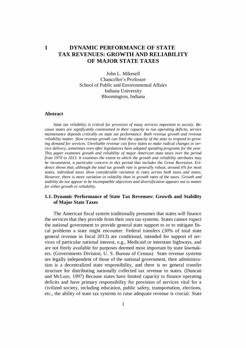
Table 5. Correlations Between Growth and Reliability Measures for To-
tal and Major State Taxes, 1970 – 2013 (Cross-Section of State
Measures, current dollar)
Total Individual
Income
General
Sales
Corporate
Net Income
Motor
Fuel
g and z -0.055 -0.664 -0.293 -0.187 -0.135
g and CV -0.1236 0.852 0.170 0.855 0.835
z and CV -0.033 -0.385 -0.198 -0.129 -0.208
There are higher correlations for the individual taxes than for total taxes.
The relationship between individual income tax growth rates and short-term
performance is generally greater than for the other taxes. Growth is negatively
related to z (r = -0.664), suggesting less volatility with higher growth or, in
other words, that annual values tend to be close to the growth path. However,
a higher growth rate is associated with a higher CV (r = 0.852), indicating
greater variation from the average as growth is higher. The direction of rela-
tionship between growth and z is also negative for general sales, corporate in-
come, and motor fuels, but the size of the correlation is not high. Similarly, the
direction of the relationship between growth and CV is positive for those taxes
as well, but the correlation is high for corporate income and motor fuel taxes,
both with r > 0.80. Higher growth is associated with more volatility for those
taxes.
The pattern for total tax revenue does not match that of the individual tax-
es. Whereas there was evidence of a relationship between growth and stability/
volatility for certain taxes, there is no such pattern for total taxes. The correla-
tion coefficient is small for both growth to stability and growth to volatility.
In terms of the tax structure as a whole, long-term and short-term patterns
do not appear to be related. The patterns identified in some of the individual
taxes do appear to be dampened when they contribute to the overall tax struc-
ture. However, Table 6 shows little correlation between diversification and
growth (r = -.220), concentration and growth (r = -.182), diversification and
volatility (r= .176), concentration and volatility (r = .119), diversification and
stability (0.127), or concentration and stability (r = -.074). Therefore, while
some of the performance for individual taxes would suggest some useful im-
pact on total tax revenues, formal measures of overall structural patterns pro-
vides no support for an influence.
6. Conclusion
This analysis of state tax revenue patterns over the 1970 to 2013 period
leads to several conclusions of significance to development of tax policy and
to the understanding of revenue behavior. The major findings may be summa-
rized:

Mikesell
20
(i) State tax portfolios have become less diversified over the past forty
years. A growing share of total collections comes from the two most
significant revenue producers, the individual income and retail sales tax-
es.
(ii) The two recessions of the twenty-first century had a particularly large
impact on the individual income and corporate net income taxes. Their
impact on total tax collections was much greater in those recessions than
in others during the past forty years.
(iii) The cyclical swing measure of relative response to national recessions is
greatest for corporate net income, individual income, and retail sales
taxes.
(iv) The average growth rate across all states for total state tax revenue was
6.6% in nominal terms and 3.3% in real terms. Among the major taxes,
the average growth rate across states was highest for individual income
and retail sales taxes and lowest for motor fuel taxes.
(v) Revenue volatility was highest for the corporate net income and individ-
ual income taxes. It was least for motor fuel taxes.
(vi) Revenue stability was greatest for the motor fuel taxes. The individual
income tax was least stable.
(vii) There is no evidence that higher growth and lower volatility are incom-
patible.
(viii) There is no evidence that diversification improves growth rates, reduces
revenue volatility, or increases revenue stability.
REFERENCES
Duncan, Harley T. and Charles E. McLure (1997) “Tax administration in the
United States of America: a decentralized system,” Bulletin for International
Fiscal Documentation, 51(2):74-85.
Dye, Richard F., and Therese J. McGuire (1991) “Growth and Variability of
State Individual Income and General Sales Taxes,” National Tax Journal,
44:55-66.
Friedenberg, Howard, and Robert Bretzfelder (1980) “Sensitivity of Regional
and State Nonfarm Wages and Salaries to National Business Cycles 1948-79,”
Survey of Current Business 60:26-28.
Mikesell, John L. (2015) “Changing State Revenue Strategies,” in Marilyn
Marks Rubin and Katherine G. Willoughby, eds., Sustaining the States, Boca
Raton, Florida: CRC Press, 44.

Dynamic performance of state tax revenues 21
U. S. Bureau of Census, Governments Division, Annual Survey of State Gov-
ernment Tax Collections.
[http://www.census.gov/govs/statetax/historical_data.html]
U. S. Bureau of Census, Governments Division, 2013 Annual Survey of State
Government, STC003 State Government Tax [www.census.gov]
Wildasin, David (2007) “Preemption: Federal Statutory Intervention in State
Taxation,” National Tax Journal, LX:649-662.
Williams, William V., Robert M. Anderson, David O. Froehle, and Kaye L.
Lamb (1973) “The Stability, Growth, and Stabilizing Influence of State Tax-
es,” National Tax Journal, XXVI:267–274.

22
2 ETHICAL CONSIDERATIONS IN
PUBLIC PROCUREMENT: THE CASE OF
THE SOUTH AFRICAN PUBLIC SERVICE
David Fourie
School of Public Management and Administration
University of Pretoria
ABSTRACT
A country’s public procurement practices to ensure the delivery of goods and services
should display the necessary integrity to achieve best value for the country’s citizens. Howev-
er, procurement fraud is frequently committed – such abuses have been widely reported and
researched. This kind of fraud is believed to be one of the most common and costly of all white
collar crimes globally. Such fraud has become increasingly elaborate and the public and pri-
vate sectors are left to face the cost repercussions and accountability concerns. Despite the
legislation developed and implemented to counteract corruption and the public sector agen-
cies created to combat it, corruption seems to be increasing. Corruption in public procure-ment can often only be detected once it is reported. Perhaps it is time to investigate the con-
struct of ethical conduct in public procurement to direct human effectiveness towards the
principles of sound ethical behavior.
Key words: public procurement, corruption, ethical considerations, procedural ethics, detect
procurement corruption
JEL Classification: H:57
1. INTRODUCTION
Government at all levels, and the private sector all over the world, has al-
ways had to face the challenges of corruption. In South Africa, the elements of
an effective anti-corruption framework are in place, but the framework does
not function optimally and is not adhered to sufficiently to make it effective.
Hence, South Africa’s levels of corruption and perceptions of corruption con-
tinue to rank amongst the highest in the world: according to Transparency In-
ternational’s Corruption Perception Index for 2014, South Africa is rated
number 67 out of 174 countries (Transparency International, 2015, n.p.). There are inefficiencies within and between institutions with anti-corruption
mandates. The system is also weakened by a lack of effective follow-up on
complaints of corruption and inefficient application of disciplinary systems,
underdeveloped management capacity in some areas, and societal attitudes
which undermine anti-corruption efforts. Corrupt acts by public servants in
particular contribute directly to the increase in the levels of corruption in
South Africa.

Ethical considerations in public procurement 23
Ethical conduct is important in any democracy to ensure that society trusts
and has confidence in the actions and decisions taken by government. There-
fore, this paper focuses on ethical considerations in public procurement from a
South African perspective. The Constitution of the Republic of South Africa
(RSA, 1996) is the country’s supreme law, and for this reason the constitu-
tional procurement principles form the basis of the study. Public procurement
terminology is clarified, as there are numerous differences in definitions. Var-
ious methods of procurement and types of and manifestations of corruption in
public procurement are analyzed. Finally, attention is paid to procurement and
ethical considerations relating to administrative measures, regulatory measures
and social measures.
The method of investigation used is a qualitative analysis investigating
relevant legislation and policy documents developed by the South African Na-
tional Treasury and the South African Public Service Commission.
2. CONCEPTUAL FRAMEWORK OF PUBLIC PROCUREMENT
Public procurement is a key economic activity of every government. It
represents a large portion of a country’s Gross Domestic Product (OECD,
2009:9). For this reason, public procurement must be recognized as a function
that generates comprehensive financial activity in most countries.
Different authors attach different meanings to the term “procurement”. It is
referred to, amongst other things, as a business function with an economic ac-
tivity, a business process in a political system, and a strategic profession.
Sherman (1991:9) defines procurement as “a business function charged with
and qualifying external sources, forming agreements, and administering them
so that material and services that enhance the work of the organization are re-
liably delivered”. As an economic activity, procurement refers to the economic
relationship between a vendor and a purchaser and, to the extent that transac-
tions occur in the context of a market order, that relationship is determined by
the laws of the market (Trepte, 2004, p. 5). According to Beste (2008, p. 12),
procurement is also a management function carried out proactively as a value-
adding process by a specialized purchasing department or unit.
De la Harpe (2009, p. 25) prefers the definition of procurement provided
by the African Development Bank, which sees procurement “as a process of
acquiring goods, works and services resulting in the award of contracts under
which payments are made in the implementation of projects, in accordance
with the governing rules and procedures and guidelines of the financing agen-
cy or agencies”.
The term “acquisition” is often used to describe the process, whereas the
term “procurement” is used for a specific acquisition activity, according to the

24 Fourie
Public Administration Leadership and Management Academy, 2011 (RSA,
2011, p. 20-21). Lyson and Gillingham (2003, p. 5) also consider the differ-
ence between “purchasing and procurement”, and claim that purchasing is the
acquisition of goods or services in return for a monetary or equivalent pay-
ment. From their differentiation it can be concluded that purchasing is the “ac-
tion”, and procurement is the “process or method” followed.
Linarelli (2011:773) argues that governments must protect their citizens in
a global economic crisis by implementing fiscal policy to counteract economic
downturns. The manner in which a government reacts to a crisis is often re-
flected in its procurement decisions. For example, in 2005, the American gov-
ernment’s response to Hurricane Katrina was to raise the “micro purchase
threshold” to $250,000 for the procurement of goods and services (Schwartz,
2011, p. 807). According to Schwartz (2011, p. 807), the measures that the
American government implemented “were an exercise in political iconography
– induced by the desire to appear to be taking decisive action promptly to ad-
dress genuine suffering.”
The American Recovery and Reinvestment Act of 2009 (cited in Linarelli,
2011, p. 773) is a good example of the interaction between public procurement
and the economy. The Act states that no funds appropriated by the United
States of America Congress may be used on the “construction, alteration, or
repair of public buildings or public works unless all of the iron, steel, and
manufactured goods used in the project are produced in the United States.”
Although the Act has a negative economic effect on countries such as Brazil,
which exports steel to the USA, the Act provides economic justice to Ameri-
can citizens (Linarelli, 2011, p. 773). Some countries also use procurement in
a proactive way – according to Dagbanja (2011, p. 34), procurement can be
used as a tool for industrial policy, to preserve jobs and profits in national in-
dustry and to promote development in particular sectors.
South Africa has also designated sectors for specific attention in order to
achieve social and economic goals. In sectors such as tourism, construction
and textiles, stipulated minimum thresholds for local production and content
apply. Tenders that fail to adhere to a stipulated minimum threshold are liable
to be ruled “not to specification” and such tender are then rejected (RSA: Na-
tional Treasury, 2011, p. 5). The sheer volume of government spending on
public goods and services molds and influences the economies of both local
and internal entities. The South African government has also identified public
procurement as a key mechanism to achieve secondary economic objectives,
such as bridging the gap between the first and second economy created by the
apartheid system (Van Vuuren, 2006, p. 2).

Ethical considerations in public procurement 25
Electronic procurement is “an electronic process which allows contracting
authorities to utilize techniques available to the private sector in order to pro-
cure supplies or services of a repetitive nature” (Bovis, 2007, p. 99). Although
using technology tends to be expensive, its advantages, such as accuracy, bet-
ter record-keeping and readily available information, contribute towards more
cost effective and transparent resources management (Van der Walt, 2012, p.
26). Bovis (2007, p. 99) also argues that electronic procurement allows effi-
ciencies to be achieved in time and in financial terms. Electronic procurement
can assist suppliers to become global competitors. In that case, according to
Wittig, government can act as an “incubator” to help build demand for “state-
of-the-art” technology (Wittig, 2003, p. 7).
When procurement is used as a social tool, procurement preference allows
tax money to be returned to domestic residents, create more jobs, and reduce
imports (Miyagiwa, 2006, p. 346). Arrowsmith (1996, p. 11) suggests that the
protection of some industries is largely a political consideration, rather than a
genuine way to address economic concerns. South Africa has a history of dis-
criminatory and unfair practices, where certain groups were marginalized and
prevented from accessing government contracts (Bolton, 2006, p. 19, 4). In an
effort to address these imbalances, the Preferential Procurement Policy
Framework Act, 5 of 2000 (RSA, 2000c), was approved. Procurement prefer-
ence is used as a tool in developing countries, and it is also a reality in devel-
oped countries. However, Arrowsmith (1996, p. 11) criticizes the protection of
industries, because it perpetuates “infant” industries where “the infant never
outgrowths its infancy, and preference and subsidies tend to be extended
through adolescence, adulthood and premature senility”.
3. METHODS OF PROCUREMENT
Public procurement should preserve integrity, and best value must ulti-
mately be achieved. Dagbanja (2011, p. 133) defines best value as “the provi-
sion of economic, efficient and effective services, of a quality that is fit for
purpose, which are valued by their customers, and are delivered at a price ac-
ceptable to the taxpayers who fund them”.
For transparency reasons, most countries use “open and selective” tender-
ing, where tenders must be advertised, and competition is encouraged. Compe-
tition for public contracts is expected to force suppliers to offer competitive
prices and services on attractive terms (Hjelmborg, Jakobsen and Poulsen,
2006, p. 23). Limited tendering is not encouraged, since only a few tenderers
are contacted (and in some instances only one tenderer is contacted) (Ar-
rowsmith, 2011, p. 292). The Organisation for Economic Co-operation and
Development (OECD) describes “open tendering” as a procurement method
where all interested suppliers may submit a tender, whereas “limited tender-

26 Fourie
ing” refers to a procurement method where the entity contacts supplier(s) indi-
vidually (OECD, 2009, p. 137-138).
A number of practices may be beneficial in order to ensure sound pro-
curement integrity. These include the prequalification of tenderers in order for
the purchasing entity to ascertain which tenderers have the required abilities
and capabilities to execute the contract (Arrowsmith, 2011, p. 308; Dagbanja,
2011, p. 111; RSA: National Treasury, 2004, p. 41). In the two-stage tendering
method, tenderers put their tender price in one envelope, and their suggested
methodology or functionality in a second envelope. Functionality is evaluated
first, before the price envelopes of the tenderers that are most likely to satisfy
the needs of the procuring entity are opened. The aim of two-stage bidding is
to prevent price from influencing the decision, with due consideration of cost
effectiveness (Dagbanja, 2011:135; RSA: National Treasury, 2004:33).
In South Africa, urgent and emergency procurement are also recognized,
where an emergency necessitates immediate action in order to avoid a danger-
ous or risky situation or misery (RSA: National Treasury, 2004:31). Extreme
urgency may be brought about by events unforeseen by the authorities award-
ing the contracts, and by the time-limit laid down in other procedures, and
then the normal approved procedures cannot be kept (De Koninck and Ronse,
2008, p. 270). However, the circumstances giving rise to the urgency should
not be foreseeable and should also not be the result of dilatory conduct by the
procuring entity (Arrowsmith et al., 2000, p. 549).
With procurement in terms of functionality, if the purchasing authority
wishes to award a contract based on factors other than price, the criterion of
“the most economically advantageous tender” must be used. Functionality re-
quires the purchasing authority to take into account elements such as quality,
reliability, viability, properties, environmental considerations and the durabil-
ity of a service, and the bidder’s technical capacity and ability to execute a
contract (Bolton, 2007, p. 107; Hjelmborg et al., 2006, pp. 230-231; RSA: Na-
tional Treasury, 2011, p. 4).
Negotiation as a method is described by Lyson and Gillingham (2003, p.
626) as “the process whereby two or more parties decide what each will give
and take in an exchange between them”. Their understanding is in line with
that of Hugo, Badenhorst-Weiss and Van Biljon (2006, p. 236-239), who con-
sider constructive negotiations to be win-win negotiations, and argue that cost-
effectiveness, changes in specifications and post-tender negotiations form the
basis of such negotiations. Allowing negotiation should not allow bidders a
second or unfair opportunity, to the detriment of any other bidder, and it
should not lead to higher prices (Bolton, 2007, p. 460).

Ethical considerations in public procurement 27
4. KEY LEGISLATION REGULATING PUBLIC PROCUREMENT IN
SOUTH AFRICA
As the supreme law, the Constitution of the Republic of South Africa, 108
of 1996 (RSA, 1996) also lays the foundation for public procurement. Section
2 stipulates that any “law or conduct inconsistent with it [the Constitution] is
invalid”, thereby placing a responsibility on the public sector to ensure that the
laws approved and the execution of public sector activities adhere to the prin-
ciples and requirements of the Constitution. The system whereby public pro-
curement must take place is captured in section 217(1) of the Constitution,
which states that procurement must take place “in accordance with a system
which is fair, equitable, transparent, competitive and cost effective.” Cost ef-
fectiveness is strategically placed as the last principle against which all other
principles must be measured. Section 217(2) of the Constitution also allows
for categories of preference in the allocation of contracts and the protection or
advancement of persons (or categories of persons) disadvantaged by unfair
discrimination.
As stipulated in section 217(3), the National Treasury has enacted the
Preferential Procurement Policy Framework Act, 5 of 2000 (RSA, 2000c) in
this regard. Chapter 10, section 195 of the Constitution (RSA, 1996) refers to
the “Basic values and principles governing public administration”. Sections 32
and 33 of the Constitution (RSA, 1996) deal with access to information and
just administrative action. These two rights were enacted in the Promotion of
Access to Information Act, 2 of 2000 (PAIA) (RSA, 2000a) and the Promotion
of Just Administrative Action Act, 3 of 2000 (PAJA). The application of the
PAIA and PAJA was highlighted in public procurement in the matter between
Millennium Waste Management (Pty) Limited and The Chairperson of the
Tender Board: Limpopo, where the judge found that because “the decision to
award a tender constitutes administrative action, it follows that the provisions
of the Promotion of Administrative Justice Act [3 of 2000 (RSA, 2000b)] ap-
plies. Of importance is that conditions used when making decisions should not
be mechanically applied with no regard to a tenderer’s constitutional rights”
(Millennium Waste Management v Chairperson Tender Board [2007] SCA
165 (RSA).
The constitutional principles of public procurement are also reflected in
the Public Finance Management Act, 1 of 1999 (PFMA) (RSA, 1999). In
terms of section 38(1)(a), which states that an accounting officer “must ensure
that the institution has and maintains” systems for the various activities listed
as part of the general responsibilities of accounting officers. Section
38(1)(a)(iii) prescribes “an appropriate procurement and provisioning system
which is fair, equitable, transparent, competitive and cost-effective”.

28 Fourie
In 2004, the Prevention and Combatting Corrupt Activities Act, 12 of 2004
(RSA, 2004) was introduced. This Act emanated from the realization that cor-
ruption and related corrupt activities undermine the rights of citizens, endan-
ger the stability and security of societies, undermine the institutions and values
of democracy, and ethical values and morality, jeopardize sustainable devel-
opment, the rule of law and the credibility of governments, and provide a
breeding ground for organized crime. In an effort to detect and prevent collu-
sive practices, the Competition Act, 89 of 1998 (RSA 1998) was introduced to
create an efficient, competitive economic environment, thereby balancing the
interests of workers, owners and consumers, and focusing on development to
benefit all South Africans.
5. PUBLIC PROCUREMENT AND CORRUPTION
The word “corruption” comes from the Latin verb corruptus (to break); it
means “broken object”. It refers to a form of behavior that departs from ethics,
morality, tradition, law, and civic virtue (Dye, 2007, p. 303). According to the
OECD (2014, p. 2-3), corruption excludes poor people from public services
and perpetuates poverty. Corruption in procurement leads to increases in the
cost of doing business, a waste of public money and resources, and inferior
quality of products and services; it can also discourage more qualified suppli-
ers from doing business with the state (OECD, 2014, p. 2-3).
On 19 December 2014, World Bank Group President Jim Yong Kim de-
scribed the pernicious effects corruption can have in developing countries as
follows:
Every dollar that a corrupt official or a corrupt business person puts in
their pocket is a dollar stolen from a pregnant woman who needs health care; or from a girl or a boy who deserves an education; or from communities that
need water, roads, and schools. Every dollar is critical if we are to reach our
goals to end extreme poverty by 2030 and to boost shared prosperity (World Bank, 2013, n.p.).
The prevalence and style of corruption in public procurement vary consid-
erably between countries, and they also impact on society on various levels.
Corruption jeopardizes the ability of governments to achieve their agenda, af-
fects spending on priority sectors such as education and health, and can have a
damaging impact on growth (Dorotinsky and Pradhan, 2007:267; Paterson and
Chaudhuri, 2007:159). Public procurement is particularly susceptible to cor-
ruption, due to the large amount of public funds involved in procurement, and
the discretion that public officials, politicians, and parliamentarians have over
public procurement (Ware et al., 2007, p. 296).
A distinction can be made between benefits that are paid willingly (brib-
ery) and payments that are extracted from unwilling clients (extortion)

Ethical considerations in public procurement 29
(Tanfa, 2006, p. 12). According to Prier and McCue (2006, p. 15-18), there are
two kinds of corruption: grand corruption and petty corruption. O’Donnell
(2008, p. 225) sees administrative corruption as petty corruption and identifies
bribery as an example. Bribery can occur to support fraud, to avoid criminal
liability and in support of unfair competition for benefits or resources. Grand
corruption, such as illicit influence/influence peddling over legislation or
policy, tends to erode the system, while petty or administrative corruption is
usually practiced by bureaucrats in a manner that threatens the efficiency of
governing institutions (O’Donnell, 2008, p. 228). Practical examples of brib-
ery include “where officials are paid by firms to be ‘short listed’ or prequali-
fied, to win contracts, to approve contract amendments and extensions, to in-
fluence auditors, to induce site inspectors to compromise their judgment re-
garding quality and completion of civil works, and to avoid cancellation of
contracts due to poor performance.” Kickbacks are taken when a successful
bidder makes a payment to a third party that acts as an intermediary for the
corrupt parties (Paterson and Chaudhuri, 2011, p. 163; OECD, 2009, p. 95).
Tanfa (2006, p. 11) discusses Advance Fee Fraud. This includes misre-
presentation, corruption and bribery. It is defined as “an upfront payment, by a
victim to a fraudster, to allow him to take part in a much larger financial trans-
action … which he believes will either bring him profit or will result in credit
being extended to him”. Another form of corruption is coercive practices.
This method of corruption “means harming or threatening to harm, directly or
indirectly, persons or their property to influence their participation in a pro-
curement process, or affect the execution of a contract” (United Nations office
on Drugs and Crime, 2008, p. 3). Various names (concepts) given to the vari-
ous methods of corruption make it difficult to develop methods and systems to
detect and prevent corruption in public procurement.
In the South African context, for example, the Minister of Finance report-
ed on 14 October 2014 that the public sector wage bill for 2014-2015 was
R439-billion and that approximately 1,3 million people were employed by the
national and provincial governments. In that year, at least R30-billion was lost
due to corruption in the procurement of goods and service and in the construc-
tion industry. This amounts to a staggering R23,076.92 (1,846.08 US$) aver-
age per public servant during the 2014-2015 financial year. According to Sta-
tistics South Africa (2013, p. 2), the South African population was estimated
at 52 million in 2013. The cost of corruption per South African citizen was
R566,25 over the same period (Maswanganyi, 2014:8). See Figure 1 reflecting
the corruption index.
According to the 2014 Corruption index (http://mg.co.za/article/2014-12-
02-fsdf), South Africa scored 44 out of 100 and is ranked 67 of the 174 sur-
veyed countries and territories. Countries are scored on a scale from 0 – 100,
with 0 representing most corrupt and 100 very clean. Since 2012, South Africa

30 Fourie
has consistently scored below 50. In 2012 and 2013, the country scored 43 and
42 respectively, with rankings of 69 out of 174, and 72 out of 177. The index
is the most widely used indicator of corruption worldwide. According to Cor-
ruption Watch (http://mg.co.za/article/2014-12-02-fsdf) these figures therefore
highlight the gradual erosion of trust in South Africa’s public sector.
Figure 1. Corruption Index
Source: (http://mg.co.za/article/2014-12-02-fsdf - Accessed on 1 April 2015).
Transparency International reported that, according to its 2013 “Global
Corruption Barometer”, on average, 27% of people reported that they had paid
a bribe for the period from 2012 to 2013. However, the percentage for South
Africa over the same period averaged 40% to 49%. Other countries listed in
the same category are Algeria, the Democratic Republic of the Congo and Ni-
geria (Hardoon and Finn 2013, p. 9).
Corrupt activities can only be prosecuted after the deed has taken place,
but the key to good service delivery is actually prevention (UNODC, 2013:2).
In an effort to limit collusion amongst parties, the South African National
Treasury introduced SBD 9 (the Standard Bidding Document) to be completed
by all prospective bidders (RSA, National Treasury, 2010). Bidders are re-
quired to sign a “Certificate of independent bid determination” and submit it
together with their bid documents (RSA: National Treasury, 2010, p. 2).
Effective functioning of public procurement is often hamstrung by a lack
of integrity in the procurement process, a lack of effective competition be-
tween suppliers and collusion among suppliers. Integrity is defined by the
OECD (2009, p. 19) as “the use of funds, resources, assets and authority, ac-

Ethical considerations in public procurement 31
cording to the intended official purposes, to be used in line with public inter-
est”. Amundsen (2009, p. 23) adds that it involves “having a sense of honesty
and truthfulness in regard to the motivations for one’s actions”, and that cor-
ruption is the antonym of integrity.
6. PROCUREMENT AND ETHICAL CONSIDERATIONS
Despite the various forms of legislation introduced and public sector agen-
cies created to combat corruption in South Africa, corruption continues to rise.
The detection and reporting of corruption normally relies on sources such as
the Auditor-general’s reports, Internal Audit reports on where controls are by-
passed or where governance problems occur, hotline reports, records of disci-
plinary hearings and grievance procedures, media reports and whistleblowing.
The question then arises what could be done to prevent corrupt activities.
It can be assumed that ethical standards and integrity are not in line with the
standards required by the Constitution, Chapter 10, which stipulates that a
“high standard of professional ethics must be promoted and maintained”
(RSA, 1996). This particular value and principle provide a firm foundation to
execute public duty in a professional and ethical manner. Ethics goes beyond
the prevention of fraud, corruption and misconduct. Ethical conduct should
aim to promote an ethical culture in discharging public duty. Williams and
Quinot (2007, p. 339) believe that resistance to corruption as a concept is
steeped in morality and ethics, and is a sensitive subject to address because of
elements of moral misappropriation, shame and wrongdoing. Bureaucratic cor-
ruption that involves government officials is a moral dilemma that is not nec-
essarily based on need, but also on greed. Dye (2007, p. 304) argues that cor-
ruption does not make economic distinctions – it infects all forms of govern-
ment; he believes that countries cannot “sustain the social, political, or, eco-
nomic costs that corruption entails”.
Ferreira (2008, p. 1) distinguishes between ethics and ethical behavior.
Ethics concerns itself with what is good or right in human interaction and re-
volves around three central concepts: “self”, “good” and “other”. Ethical be-
havior results when one does not merely consider what is good for oneself, but
also considers what is good for others. Modern societies expects public serv-
ants to serve the public interest, and to serve in a rational and efficient way
(Amundsen, 2009, p. 11). Ferreira (2008, p. 2) adopts a definition referred to
by Flowers (2002), who describes ethics as “the ability to think clearly and
critically through a challenging problem, and to understand the difference be-
tween what one has a right to do, and the right thing to do”.
In psychology, two schools of thought express strong views on ethics.
Psychoanalysts claim that each individual’s good and evil behavior is a result
of actions taken and desires repressed in order for an individual to function in

32 Fourie
society. Behaviorists believe in the power to change human nature by arrang-
ing conditions to be favorable to the desired changes (Fox, 2010, p. 37). The
question then arises whether codes of conduct for public servants influence
human nature and compel public servants to apply constitutional principles in
the execution of their functions. Codes of conduct are often government’s re-
sponse to citizens’ expectations around trust, responsibility, and accountabil-
ity. In the South African context, a Code of Conduct for the Public Service
was introduced in 1997. This Code sets standards for ethical conduct. The
Code is supported by the Financial Disclosure Framework, which requires
senior officials to declare their financial interests on an annual basis.
Fox (2010, p. 4) indicates that he agrees with Convey (1992) that there are
fundamental principles that direct human effectiveness, principles such as
fairness, integrity, honesty, human dignity, service, quality, excellence, poten-
tial and growth. Ferreira (2008, p. 2) also supports Sullivan’s (1995) argument
that integrity is never a given, but is always a quest that must be renewed and
reshaped over time. It demands considerable individual self-awareness and
self-command.
Fairness as a fundamental principle relates to getting what a person de-
serves: due process and just allocation (Pauw and Wolvaardt, 2009:71-73).
Granville and Dine (2013, pp. 5-7) suggest that there is an emotional dimen-
sion to fairness and that it is pointless to get caught up in platitudes such as
“from each according to his ability, to each according to his needs”. Fairness
in public procurement is an obligation of the public sector where administra-
tive reasonableness can be tested against procedural fairness. The judgment in
Laingville Fisheries (Pty) Ltd v The Minister of Environmental Affairs and
Tourism (C) states:
Factors relevant to determining whether a decision is reasonable or not will
include the nature of the decision, the identity and expertise of the decision-maker, the range of factor relevant to the decision, the reasons given for the
decision, the nature of the competing interests involved and the impact of the
decision on the lives and well-being of those affected.
Administrators and bureaucrats cannot avoid making decisions, and their
discretionary powers require them to consider the ethical dimension of their
decision-making (Amundsen, 2009, p. 5).
Denton (1991, p. 2) asks whether ethical politics are possible, or whether
ethical politics is an oxymoron. Elected officials are expected to act for the
common good of the entire nation, although their jobs might require them to
lie about information or actions. Denton’s reflection is concerning, since elect-
ed officials can become selective in terms of transparency, which is a prereq-
uisite for accountable government. Discussions on good governance seldom
include the professional and personal ethics of politicians and of elected office

Ethical considerations in public procurement 33
holders (Amundsen, 2009, p. 5). Politicians have a great deal of power and
influence, and they control the raising and spending of public money, adminis-
ter and enforce laws, and possess the ability to choose when to go to war (Pot-
ter, 2006, p. 74).
External demands on public procurement are great and varied. They in-
clude transparency, integrity, accountability and exemplary behavior, where
government is expected to set an example of ethical standards, efficiency and
effectiveness in its operations, as expected by the broader society (Telgen,
Harland and Knight, 2007, p. 245). With limited financial resources, ethical
dilemmas often arise in deciding about who the beneficiaries of public goods,
works or services are to be.
A distinction between ethical dilemmas and moral temptations must be
made. Ethical dilemmas consist of conflicts between right and right, while
moral temptation consists of a conflict between right and wrong. A moral
temptation arises when stimulation of economic activities may bolster an indi-
vidual’s chances of reelection. Ware et al., (2007, p. 296) refer to these pro-
jects of parliamentarians as “pork-barrel” projects.
Currie and De Waal (2005, p. 680) argue that although transparency in-
creases consistency, it also reduces flexibility. Flexibility is often necessary
when the development of specific economic sectors depends on where gov-
ernment procures goods and services (Doyle, 2001, p. 217). Pauw and
Wolvaardt (2009, p. 68) suggest that a trade-off between principles such as
transparency, accountability, effectiveness, participation, efficiency, propor-
tionality, consistency and coherence can be in conflict with consistency and
coherence, as identified by Roos and De la Harpe (2008, p. 5). According to
them too much transparency may hamstring competition, and considering too
many tenders can reduce cost-effectiveness. Similarly, Amundsen (2009, p.
21) argues that the financial cost of and time consumed in providing access to
information can be higher than the practical use of the information, and adds
that little transparency in a corrupt setting can assist in revealing who is “up
for sale”. The OECD (2007, p. 11) states that although transparency and ac-
countability have been recognized as key conditions for promoting integrity
and preventing corruption, they must be balanced with administrative efficien-
cy.
Competition is considered a core objective for procurement systems which
is essential to good performance (Anderson and Arrowsmith, 2011, p. 682).
Although the Constitution in South Africa prescribes a competitive system,
Bolton (2007, p. 46) is of the opinion that not using competitive procedures
does not necessarily mean that value for money cannot be attained. For in-
stance, if there are only four suppliers in the market, is it cost-effective to use
an expensive open bid method? Inviting only the four bidders to submit a ten-

34 Fourie
der is still transparent and open, as long as adequate written reasons can be
given. Administrators should determine adequacy on a case-by-case basis
(Currie and De Waal, 2005, p. 679).
7. ATTAINMENT OF ETHICAL CONDUCT
William and Quinot (2007, p. 343) identify accounting and audit require-
ments as administrative processes or measures that can address corruption.
Dye (2007, p. 304) argues that audit staff tend to demand strict compliance
with procedures, while missing the objective of compliance. In South Africa,
the heads of public institutions are given the power to restrict suppliers from
doing business with the public sector if such suppliers obtain preference
fraudulently (RSA, National Treasury, 2006, p. 1).
Functionaries can play an active role in the attainment of ethical standards
in public procurement. They should promote and maintain the highest stand-
ards of probity and integrity in all their dealings. For this reason, special atten-
tion should be given to the screening of prospective employees in the ap-
pointment process and the creation of codes of conduct (UNODC, 2013, p. 11)
and the enforcement of the Code of Conduct for the Public Service as intro-
duced in 1997. Screening assists in identifying possible conflict of interest,
and whether an applicant has the essential skills to perform the required func-
tion effectively and has the insight to detect corrupt activities. Performance
results need to improve across government, hence there is a need for a variety
of training forms to address performance issues at the individual level and at
an institutional level. In response to the South African government’s commit-
ment to improving performance results, 199 281 officials were trained from
2009 to 2014 on various matters relating to the public sector. Despite this
achievement, the training has not yet yielded the anticipated positive results in
preventing public procurement corruption and thus ethical conduct, as is evi-
dent from the latest Corruption Index (RSA, School of Government, 2014).
Disoloane (2012, p. 92) argues that a code of conduct fulfils a primary
function in the fight against corruption and unethical behavior on the part of
public officials and political office-bearers. The goal of codes is to establish an
ethical culture and high standards of integrity within departments and ulti-
mately the public service. But codes should not just be something produced on
paper – they should involve submission to moral codes of integrity and should
be a condition of employment (RSA, Department of Public Service and Ad-
ministration, 2013, p. 4).
Public and private sector employees are usually the first to identify wrong-
doing in the workplace and are considered the most useful and reliable re-
sources in exposing corrupt practices. In environments where reporting of
wrongdoing is not protected, the risk of corruption is significantly higher

Ethical considerations in public procurement 35
(OECD, 2012, p. 3). Hardoon and Finn (2013, p. 23) conducted a survey in
107 countries on the reasons people give for not reporting incidents of corrup-
tion. When asked why they did not report corruption, 15% of respondents in-
dicated that they did not know where to report it, 35% were afraid of reprisals,
45% believed it would not make any difference, and 5% gave other reasons.
Governments around the world need to find methods to make ordinary people
believe that they can make a difference in preventing and detecting corruption
in the public sector. However, when they were asked to indicate which catego-
ries they perceived to be affected by corruption on a scale from 1 to 5, the citi-
zens of 107 countries rated political parties highest at 3.8, the police and pub-
lic officials at 3.7, and the judiciary at 3.6 (Hardoon and Finn, 2013, pp. 23,
16). These findings are cause for concern in any democracy. The effectiveness
of encouraging whistleblowers depends on the manner in which an organiza-
tion reacts to information, and it is imperative that organizations to respond or
take action once the whistle has been blown, even if there is a dispute as to the
legitimacy of the accusation (Disoloane, 2012, p. 103).
The Constitution of the Republic of South Africa (RSA, 1996) is the su-
preme law in creating good governance in the public service. State institutions
supporting a constitutional democracy are identified in section 181(1) of the
Constitution. In the public procurement environment, the Public Protector and
Auditor-general play an important role. The Public Protector is appointed by
the President, but is subject only to the Constitution, thereby allowing the Pub-
lic Protector to function without fear, favor or prejudice. The number of com-
plaints received by the office of the Public Protector (33 533 in 2012/13) is an
indication of society’s trust in the Office as an institution to strengthen consti-
tutional democracy in South Africa (Van der Walt, 2014:309). Whereas the
Public Protector investigates complaints from the public, the Auditor-General
is responsible for producing annual reports on the accounts and financial
statements of all organs of state in the national, provincial or local spheres of
government and other public entities. These audits include the assessment of
procurement processes, contract management and verification of the controls
in place to ensure fair, equitable, transparent, competitive, and cost-effective
Supply Chain Management systems.
Whistleblowing as a source of the detection and elimination of corrupt re-
lationships fulfills an important role too. It is a mechanism whereby a person,
either internal or external to an organization, draws attention to wrongdoing
within an organization. Such reporting is mostly facilitated by hotlines. Whis-
tleblowing is also defined as not being about informing in the negative, anon-
ymous sense, but rather about raising a concern about malpractice within an
organization. Whistleblowing is not necessarily applicable only in public insti-
tutions, but also in the private sector, reporting information of corrupt relation-
ships between public and private sector employees. To be effective, the in-
formants must be protected against intimidation, harassment, dismissal or, in

36 Fourie
some instances, violence. In South Africa, protection takes place through the
Protected Disclosure Act, 6 of 2000 (RSA, 2000d).
In South Africa, the Code of conduct for supply chain management practi-
tioners reflects the required conduct expected from functionaries in respect of
conflict of interest, accountability, openness and confidentiality. Not only does
this Code provide the responsibilities of Bid evaluation and Bid adjudication
teams, but it also places an obligation on institutions to ensure the clearance of
members on the level of “confidential” (RSA, National Treasury, 2003, pp. 2-
3). Verification of an official’s financial standing, interest and past practices
assist accounting officers in selecting committee members who are above re-
proach
Legislation allows for precautionary suspension of employees that serves
as a safety measure used by affected departments to allow for unhindered in-
vestigation pending the institution of disciplinary procedures. In terms of
South Africa’s Disciplinary Code and Procedures (Resolution 1 of 2003),
public institutions have 60 days within which a hearing should be held. Ac-
cording to the Department of Public Service and Administration for the period
2009/2010, the combined amount remuneration paid to employees placed on
precautionary suspension was more than R45 million (South Africa. Public
Service Commission, 2011, p. 12).
Officials’ resigning whilst on suspension often results in corrupt officials’
being appointed in other government institutions before investigations are fi-
nalized. Delays in finalizing instituting disciplinary actions have a negative
financial effect on the state, and on government’s ability and commitment to
take decisive steps to combat corruption
Social measures refers to the disapproval that society expresses of corrup-
tion, which may include shaming, ridiculing and disgracing a person when
corruption is exposed (Williams and Quinot, 2007, p. 345). According to
South Africa’s National Development Plan, (2014, p. 1) the vision for the
country in 2030 is a society with zero tolerance for corruption in which citi-
zens do not offer bribes and have the confidence and knowledge to hold public
and private officials to account, and in which leaders have integrity and high
ethical standards (RSA, Department of Communication, 2014, p. 1). In a paper
entitled “Closing banks for the corrupt”, De Simone and Fagan (2014, pp. 1-2)
identify banks as a loophole that prevent the detection of corruption. Ill-gotten
gains easily find their way back into society via banks that legitimize income.
Grand corruption can be stopped when the corrupt do not have a safe haven
for money gained through corrupt activities. Politically-Exposed Persons
(PEPs) are defined as including “high ranking officials from government,
heads of state, senior politicians, the military and state owned companies”
(Ahlers, 2013, p. xvii). Banks can identify PEPs, scrutinize their funds, closely

Ethical considerations in public procurement 37
monitor their transactions and report suspected irregularities (De Simone and
Fagan, 2014, pp. 1-2). The monitoring of PEPs is a daunting task if money is
paid into the accounts of relatives, friends, the family trusts of the corrupt, or
when actual money does not change hands but movable or non-movable assets
are obtained for both the corrupt and those who can benefit from their posi-
tion. Professional registered companies such as financial brokers, tax consult-
ants, registered auditors should be compelled to work towards their clients’
best financial interests, but also to recognize that those hurt most by corruption
are also the most vulnerable, the people who depend, ironically, on PEPs for a
better life. Ahlers’s (2013, p. iii) research suggests that PEPs are not adequate-
ly monitored in South Africa, and the risk that the presence of corrupt political
exposed persons poses for society is not addressed adequately.
Where corruption becomes the norm, society expects that kind of behavior
from those who are in power and on whom they are forced to rely. To combat
corruption, the non-profit organization Corruption Watch was launched in
2012. It is an organization that provides a platform for reporting corruption. It
investigates reports, identifies and monitors corruption hot spots and mobilizes
ordinary people to take a stance against corruption. When necessary, the or-
ganization also acts as a friend to the court (Corruption Watch, 2014,:n.p.).
Lead SA (2015,:n.p.) is a Primedia Broadcasting initiative which aims to mo-
bilize and inspire active citizenry and leadership to make South Africa a better
country for all who live in it. Social measures also include those contributors
that not only report corruption but also assist towards curbing corruption. The
Ethics Institute of South Africa (n.d.) (EthicsSA) is a non-profit, public benefit
organization that commenced operations in August 2000 with the aim of
building an ethically responsible society by forming partnerships with the pub-
lic and private sectors, and the professions. Government institutions have their
own mediums to combat this problem, such as the National Prosecution Hot-
line (0800 21 25 80), which is operated by an independent organization. Anon-
ymous information can also be given (National Prosecuting Agency, n.d.).
As is the case with most modern governments, a variety of mediums are
available for participation by society in detecting and preventing corruption.
Society should be informed on various levels, starting at school level, of the
benefits of participation, but government should also earn trust by actively in-
vestigating and prosecuting transgressors.
8. CONCLUDING REMARKS
Corruption remains a strong challenge to good governance as it has eco-
nomic, political and social consequences for a nation. Corruption has an im-
pact on stability, and limited resources are often spent on commissions inves-
tigating corruption. Despite efforts such as training and strategic partnerships,
corruption and its cost to society continue to increase. Is corruption increasing

38 Fourie
because more officials are being appointed to serve the public, or is corruption
a symptom of the malaise of South African society? The exposure of corrup-
tion sometimes has unintended consequences, resulting in a “catch 22” situa-
tion. If a government reveals corruption, the revelation itself can be politically
destabilizing, and have negative consequences at the polls and on investment
confidence. In a corrupt relationship there are always two parties, the corrupt
and the corruptor, who share a mutually beneficial relationship (usually a fi-
nancial benefit). Society as the intended receiver of goods and services is the
victim of this relationship, when tax payers’ money is used to fund corrupt re-
lationships, and then to prevent and detect corruption. A partnership between
government and society would be the most cost-effective and sustainable tool
to eradicate corruption.
Education and training should to be used to sensitize and create a sense of
ethical conduct in the work place. Political appointees need to be vetted by
committees of the legislature, and the Declaration of Assets should be applica-
ble to all levels of managers and not only to senior officials. There should also
be a rotation system where committee members are announced only on the day
of tender decisions, as it might assist in closing opportunities for unethical
conduct in the process.
This paper offers an understanding of the issues in the public procurement
process and of underlying factors relating to procurement and ethical consid-
erations. The successful application and practice of ethical conduct in a public
organization requires strong leadership, as ethics should not be managed mere-
ly as a compliance exercise. It requires the will and ability of public leaders
and managers to set a vision which is based on generally accepted values. Eth-
ical conduct in public procurement could be subjected to detailed scientific
investigation in order to gain a clear understanding of the value of ethical con-
duct in combating corrupt activities.
REFERENCES
Ahlers, C. (2013) The South African anti-money laundering regulatory
framework relevant to politically exposed persons, Unpublished MPhil thesis,
University of Pretoria, Pretoria, South Africa.
Amundsen, I. (2009) Introduction to Public Sector Ethics, Bergen: Christian
Michelsen Institute.
Anderson, R.D. and Arrowsmith, S. (2011) “The WTO on government pro-
curement”, in: S. Arrowsmith and R.D. Anderson (eds) The WTO Regime on
Government Procurement: Challenge and Reform, pp. 3-58, USA: Cambridge
University Press.

Ethical considerations in public procurement 39
Arrowsmith, S. (1996) The Law of Public and Utilities Procurement, London:
Sweet & Maxwell.
Arrowsmith, S., Linarelli, J. and Wallace, D. 2000. Regulating public pro-
curement: national and international perspectives. Bedfordshire: Kluwer Law
International.
Arrowsmith, S. (2011) “The revised agreement on procurement: Changes to
the procedural rules and other transparency provisions” in: S. Arrowsmith and
R.D. Anderson (eds) The WTO Regime on Government Procurement: Chal-
lenge and Reform, pp. 285-336, USA: Cambridge University Press.
Beste, T. (2008) Greening the Supply Chain in Public Procurement. A Case
Study of a UK Local Authority, Saarbrücken: VDB Verlag Dr. Müller.
Bolton, P. (2006) “Government procurement as a policy tool in South Africa”,
Journal of Public Procurement, 6(3): 193-217.
Bolton, P. (2007) The Law of Government Procurement in South Africa, Dur-
ban: Lexisnexis Butterworths.
Bovis, C.H. (2007) EU Public Procurement Law, Cheltenham: Edward Elgar.
Currie, I. and De Waal, J. (2005) The Bill of Rights Handbook, 5th ed, Cape
Town: Juta.
Corruption Watch (2014a) Who we are and what we do. [Online] Available at:
http://www.corruptionwatch.org.za/content/who-we-are-and-what-we-do
(Accessed on April 19, 2015).
Corruption Watch (2014b) Economic impact of corruption. [Online] Available
at: http://www.corruptionwatch.org.za/content/economic-implications (acces-
sed on April 1, 2015).
Dagbanja, D.N. (2011) The Law of Public Procurement in Ghana, Saarbrück-
en: Lap Lambert Academic.
De Koninck, C. and Ronse, T. (2008) European Public Procurement Law: The
European Procurement Directives and 25 Years of Jurisprudence by the
Courts of Justice of the European Communities: Text and Analysis, Bedford-
shire: Kluwer Law International.
De la Harpe, S.P.L. (2009) Public Procurement Law: A Comparative Analysis,
Unpublished LLD thesis, University of South Africa, Pretoria, South Africa.

40 Fourie
Denton, R.D. Jr. (1991) Ethical Dimensions of Political Communication, New
York, NY: Praeger.
De Simone, M. and Fagan, C. (2014) Closing Banks to the Corrupt: The Role
of Due Diligence and PEPS, Berlin: Transparency International.
Disoloane, V.P.P. (2012) Reception of a Code of Conduct at the Capricorn
District Municipality in the Limpopo Province, Unpublished Ph.D. thesis,
University of South Africa, Pretoria, South Africa.
Dorotinsky, W. and Prodhans, S. (2007) “Exploring corruption in public fi-
nancial management”, in: J.E. Campos and S. Pradhan (eds) The Many Faces
of Corruption. Tracking Vulnerabilities at the Sector Level, pp.267-294,
Washington, DC: World Bank.
Doyle, M. (2001) “Public procurement and inventory management”, in: G. van
der Waldt, D. van Niekerk, M. Doyle, A. Knipe, and D. du Toit (eds) Service
Excellence in Governance, pp. 199-226, Johannesburg: Heinemann.
Dye, K.M. (2007) “Corruption and fraud detection by supreme audit institu-
tions”, in: A. Shah (ed.) Performance Accountability and Combating Corrup-
tion, pp. 303-321, Washington, DC: World Bank.
Ethics Institute of South Africa (2015) n.d.(a) Home page.
http://www.ethicsa.org/ (Accessed on February 16.
Ethics Institute of South Africa (2015) n.d.(b) https://www.saica.co.za/About/
AlliancePartnersandApprovedProvid-
ers/AlliancePartners/EthicsInstituteofSouthAfrica/tabid/2576/language/en-
ZA/Default.aspx (Accessed on February 16.
Ferreira, N.M. (2008) Ethical Considerations for Collection Developers: A
South African Perspective, Pretoria: University of South Africa Press.
Fox, W. (2010) A Guide to Public Ethics, Cape Town: Juta.
Granville, B. and Dine, J. (2012) The Processes and Practices of Fair Trade
Trust, Ethics and Governance. Abingdon: Routledge.
Hardoon, D. and Heinrich, F. (2013) Global Corruption Barometer. Transpar-
ency International. 8th ed. UK: Palgrave Macmillan.
Hjelmborg, S.E., Jakobsen, P.S., and Poulsen, S.T. (2006) Public Procurement
Law – the EU Directive on Public Contracts. Copenhagen: DJOF.

Ethical considerations in public procurement 41
Hugo, W.M,J., Badenhorst-Weiss, J.A. and Van Biljon, E.H.B. (2006) Pur-
chasing and Supply Management, 5th edition, Pretoria: Van Schaik.
Laingville Fisheries (Pty) Ltd and Others v Minister of Environmental Affairs
and Tourism (2008) JDR 0614(C).
Lead SA. (2015) Home page. [Online] Available at: http://leadsa.co.za/ (Ac-
cessed on February 16, 2015).
Linarelli, J. (2011) “Global procurement law in times of crises: New Buy
American policies and options in the WTO legal system”, in: S. Arrowsmith
and R.D. Anderson (eds) The WTO Regime on Government Procurement:
Challenge and Reform, Cambridge University Press.
Lyson, K. and Gillingham, M. (2003) Purchasing and Supply Chain Manage-
ment, 6th edition, London: Pearson Education.
Mail and Guardian [Online] Available at: http://mg.co.za/article/2014-12-02-
fsdf (Accessed on April 1, 2015).
Maswanganyi, N. (2014) “Nene urges wage moderation. Finance Minister tells
IMF increases will compromise headcount in SA”, Daily Dispatch, 14 Octo-
ber: 8.
Millennium Waste Management v Chairperson Tender Board (2007) SCA 165
(RSA).
Miyagiwa, K. (2006) “Oligopoly and discriminatorily government procure-
ment policy”, in: S. Evenette and B. Hoekman (eds) The WTO and Govern-
ment Procurement, Cheltenham: Edward Elgar.
National Prosecution Agency. n.d. [Online] Available at:
http://www.npa.gov.za/ReadContent470.aspx (Accessed on February 16,
2015).
O’Donnell, M. (2008) “Corruption: A rule of law agenda”, in: A. Hurwitz and
R. Huang (eds) Civil War and the Rule of Law: Security, Development, Hu-
man Rights, pp.225-260, Boulder, CO: Lynne Rienner.
Organisation for Economic Co-operation and Development (2007) Integrity in
Public Procurement. Good Practice from A-Z. Paris: OECD.
Organisation for Economic Co-operation and Development (2009) Principles
for Integrity in Public Procurement. Paris: OECD.

42 Fourie
Organisation for Economic Co-operation and Development (2012) Whistle
Blower Protection: Encouraging Reporting. Paris : OECD.
Organisation for Economic Co-operation and Development (2014) The Ra-
tionale for Fighting Corruption. Paris: OECD.
Paterson, W.D.O. and Chaudhuri, P. (2007) “Making inroads on corruption in
the transport sector through control and prevention”, in: J.E. Campos and S.
Pradhan, S (eds) The Many Faces of Corruption. Tracking Vulnerabilities at
the Sector Level, pp. 159-190, Washington, DC: World Bank.
Pauw, J.C. and Wolvaardt, J.S. (2009) “Multi-criteria decision analysis in pub-
lic procurement – a plan from the South”, Politeia, 26(1):66-88.
Potter, A. (2006) “Political ethics and responsible government”, in: D. Saint-
Martin and F. Thompson (eds) Public Ethics and Governance: Standards and
Practices in Comparative Perspective, Research in Public Policy Analysis and
Management, Volume 14, pp. 71-91, Amsterdam: Oxford.
Prier, E. and McCue, C.P. (2006) The 12th International Anti-Corruption Con-
ference: Public Procurement Analysis of Best Value in Anti-corruption Efforts,
Guatemala City, November 15–18, Paris: Transparency International.
Republic of South Africa (1996) Constitution of the Republic of South Africa,
Pretoria: Government Printer.
Republic of South Africa (1998) Competition Act, 89 of 1998, Pretoria: Gov-
ernment Printer.
Republic of South Africa (1999) Public Finance Management Act, 1 of 1999,
Pretoria: Government Printer.
Republic of South Africa (2000a) Promotion of Access to Information Act, 2
of 2000, Pretoria: Government Printer.
Republic of South Africa (2000b) Promotion of Administrative Justice Act, 3
of 2000, Pretoria: Government Printer.
Republic of South Africa (2000c) Preferential Procurement Policy Frame-
work Act, 5 of 2000, Pretoria: Government Printer.
Republic of South Africa (2000d) Protected Disclosure Act, 6 of 2000. Preto-
ria: Government Printer.

Ethical considerations in public procurement 43
Republic of South Africa Supply Chain Management Office Practice Note
Number SCM 4 of 2003. Code of conduct for supply chain management prac-
titioners, Pretoria: National Treasury.
Republic of South Africa (2004) Prevention and Combating of Corrupt Activi-
ties Act, 12 of 2004, Pretoria: Government Printer.
Republic of South Africa (2011). Supply Chain Management for Public Ser-
vice. Public Administration Leadership and Management Academy, 2011, Pre-
toria: National School of Government.
Republic of South Africa Department of Public Service and Administration
(2013) Guidelines on managing ethics in the public service, Pretoria: Depart-
ment of Public Service and Administration.
Republic of South Africa Department of Communication (2014) Media re-
lease. Government pours cold water on sensational media reports on corrup-
tion, Pretoria: Department of Communication.
Republic of South Africa Public Service Commission South Africa (2003)
Disciplinary Code and Procedures (Resolution 1 of 2003), Pretoria: Public
Service Commission South Africa.
Republic of South Africa National Treasury (2004) Guide to Accounting Of-
ficers/Authorities: Public Finance Management Act, Pretoria: National Treas-
ury.
Republic of South Africa National Treasury (2006) Practice note, 5 of 2006.
Pretoria: The National Treasury.
Republic of South Africa (RSA): National Treasury. (2010) Prohibition of re-
strictive practices: Certificate of independent bid determination: Standard
Bidding Document (SBD 9). Pretoria: National Treasury.
Republic of South Africa National Treasury (2011) Preferential Procurement
Policy Framework Act, 05 of 2000 and Regulations of 2011. Pretoria: Nation-
al Treasury.
Republic of South Africa Public Service Commission (2011) Report on man-
agement of precautionary suspension in the public service. Pretoria: Public
Service Commission.
Republic of South Africa School of Government (2014) Annual Report
2013/2014, Pretoria: National School of Government.

44 Fourie
Roos, R. and De la Harpe, S. (2008) Good governance in public procurement:
a South African case study.” ISSN 1727-3781. PER 2. [Online] Available at:
http://www.ajol.info/index.php/pelj/article/viewFile/42231/9350 (Accessed on
April 19, 2015).
Schwartz, J.I. (2011) “Procurement in times of crisis: Lessons from US Gov-
ernment procurement”, in: S. Arrowsmith and R.D. Anderson (eds) The WTO
Regime on Government Procurement: Challenge and Reform, pp. 803-829,
Cambridge, Cambridge University Press.
Sherman, S.N. (1991) Government Procurement Management, Germantown,
MD: Wordcrafters.
Statistics South Africa. (2013) Statistical release P0302. Mid-year population
estimates 2013. [Online] Available at: http://www.statssa.gov.za/publications/
P0302/P03022013.pdf (Accessed on April 1, 2015).
Tanfa, D.Y. (2006) Advance Fee Fraud, D.Litt. et Phil. thesis, University of
South Africa, Pretoria, South Africa.
Telgen, J., Harland, C., and Knight, L. (2007) “Public procurement in perspec-
tive”, in: L. Knight, C. Harland, J. Telgen, V. Khi, G. Callender, and K.
McKen (eds) Public Procurement: International Cases and Commentary,
pp.245, Oxford: Routledge.
Transparency International. (2015) Corruption Perceptions Index 2014: Re-
sults. [Online] Available at: https://www.transparency.org/cpi2014/ re-
sults#myAnchor1 (Accessed on February 16, 2015).
Trepte, P. (2004) Regulating Procurement: Understanding the Ends and
Means of Public Procurement Regulation, Oxford: Oxford University Press.
United Nations Office on Drugs and Crime (UNODC). 2008. Second Confer-
ence of the State Parties to the United Nations Convention Against Corrup-
tion: United Nations Convention Against Corruption: Implementing Procure-
ment Related Aspects, Indonesia, 28 January–1 February, 2008, Nusa Dua:
UNODC.
United Nations Office on Drugs and Crime (2013) Guide Book on Anti-
Corruption in Public Procurement and the Management of Public Finances.
Good Practices in Ensuring Compliance with Article 9 of the United Nations
Convention Against Corruption, Vienna: United Nations.

Ethical considerations in public procurement 45
Van der Walt, E.M. (2012) Innovations in South African Public Service Pro-
curement Policy: 1999-2005, MBA thesis, University of South Africa, Preto-
ria, South Africa.
Van der Walt, E.M. (2014) “Public Procurement: a bastion against corrup-
tion”, in: C. Thornhill and G. van Dijk (eds) Public Administration & Man-
agement in South Africa. A Developmental Perspective, Cape Town: Oxford
University Press.
Van Vuuren, K. (2006) Achieving Economic and Social Value Through Pro-
curement Professionalism, SAPICS 28th Annual Conference and Exhibition,
June 1–8, Sun City, South Africa.
Ware, G.T., Moss, S., Campos, J.E., and Noone, G.P. (2007) “Corruption in
public procurement a perennial challenge”, in: J.E. Campos and S. Pradhan
(eds), The Many Faces of Corruption. Tracking Vulnerabilities at the Sector
Level, p.296, Washington, DC: International Bank for Reconstruction and De-
velopment/World Bank.
Williams, S. and Quinot, G. (2007) “Public procurement and corruption: The
South African response”, South African Law Journal, 124: 339-363.
Paterson, W. D.O. and Chaudhuri, P. (2011) “Making inroads on corruption in
the transport sector through control and prevention”, in: J.E. Campos and S.
Pradhan (eds), The Many Faces of Corruption. Tracking Vulnerabilities at the
Sector Level, pp.159-190, Washington, DC: International Bank for Recon-
struction and Development/World Bank.
Wittig, W.A. (2003) “Public procurement and the development agenda”, Unit-
ed Nations Conference on Trade and Development. Geneva: Switzerland.
World Bank. (2013) “Corruption is ‘Public Enemy Number One’ in Develop-
ing Countries, says World Bank Group President Kim”, Dec. 19. [Online]
Available at: http://www.worldbank.org/en/news/press-release/2013/
12/19/corruption-developing-countries-world-bank-group-president-kim (Ac-
cessed on February 16, 2015).

46
3 INFRASTRUCTURE AND ECONOMIC GROWTH
IN SUB-SAHARAN AFRICA
ODONGO KODONGO
Senior Lecturer, Wits Business School, University of the Witwatersrand.
P. O. Box 98 Wits, Johannesburg 2030, South Africa
Email: [email protected]
KALU OJAH
Professor, Wits Business School, University of the Witwatersrand
P. O. Box 98 Wits, Johannesburg 2030, South Africa
Email: [email protected]
ABSTRACT
We examine the nexus between economic growth and infrastructure in a panel of forty
countries in Sub-Saharan Africa over the period, 2000 – 2011. We use monthly data obtained
from World Development Indicators and UNDP. We construct synthetic indexes of infra-
structure stocks and infrastructure quality which we use with several control variables to es-
timate a System GMM. Our results show that infrastructure quality significantly explains
economic growth while infrastructure stocks have no explanatory power. The results are ro-
bust to alternative panel compositions. African countries should therefore focus not on providing infrastructure bulk but improving the quality of their existing and envisaged infra-
structure stocks.
JEL Classification: H54, O11, O40, O55
1. INTRODUCTION
Broadly speaking, infrastructure1 provides services that form a part of res-
idents’ consumption bundles and augments capital and labor as an input in the
production process (Ayogu, 2007); it drives societal progress by promoting
human development and betters quality of life through improved productivity
and sustainable economic growth (Sanchez-Robles, 1998; Egert, Kozluk, and
Sutherland, 2009; Ajakaiye and Ncube, 2010). More specifically, infrastruc-
ture enhances trade and commerce, encourages cultural exchanges that can
promote national integration and reduce conflict, and eases labor mobility
(Mbaku, 2013). Research and policy analysis also point to the important role
infrastructure provision might play in the alleviation of poverty and inequality
(Ndulu, 2006; World Bank, 2006).
1. Infrastructure refers to highways and roads, mass-transit and airport facilities, telecommu-
nication facilities, gas and water supply facilities and distribution systems, electricity, educa-
tion buildings, waste treatment facilities, police, fire service, judiciary and correctional institu-
tions (Ayogu, 2007).

Infrastructure and economic growth in Sub-Saharan Africa
47
Yet, infrastructure development cannot be said to be at the optimal levels in
Africa. Indeed, governments and their various development partners are cog-
nizant of the region’s colossal infrastructure gap and its resultant adverse im-
pact on development efforts in various economic sectors. The huge infrastruc-
ture gap speaks to unexploited productive potential, which could be utilized by
upping infrastructure investments. Studies have identified substantial infra-
structure needs in the African region. In the mid-2000s, estimated annual in-
frastructure expenditure needs, over a ten-year period, ranged between of 9%
and 13% of GDP (Sachs et al., 2004; Economic Commission for Africa,
2005). At the end of the last decade, the annual infrastructure investment
needs for Africa as a whole was estimated at USD 93 billion, about one third
of which were for operations and maintenance (Foster and Briceño-
Garmendia, 2009). Since the current infrastructure spending is only about
USD 45 billion a year, the financing gap is clearly sizable (AfDB, 2013b).
The infrastructure deficit is worse in the sub-Saharan Africa region. The
relatively poor state of infrastructure in the region has also been documented
by AfDB (2011) according to which sub-Saharan Africa’s infrastructure is the
most deficient and costly in the developing world. Ascribing the high infra-
structure cost to diseconomies of scale and lack of competition, the AfDB re-
port estimates that about USD 93 billion (15% of GDP) per year will be re-
quired to fix the infrastructure gap. About half of this amount would be needed
in the power sector, where electricity access is only 25% compared with 50%
in South Asia and 80% in Latin America. The report notes that mobilizing in-
vestments in the power sector is made difficult by the financially weak institu-
tions that have an aggregate annual revenue shortfall of approximately USD 8
billion. The situation is not any better in other sectors. According to AfDB
(2011) the provision of water is falling with approximately 40% of rural
dwellers in the region lacking access to clean drinking water. Annual funding
gap in the sector is estimated at USD 11 billion, or about 50% of the total
funding needs. The sector is characterized by massive waste, losing about
USD 1 billion each year to operational inefficiencies of water utilities, another
pointer to capacity issues in the region.
Further to these dismal statistics, empirical investigations within the sub-
Saharan Africa region point to lost growth opportunities as a result of poor
infrastructure development. The landlocked nature of many sub-Saharan Afri-
can countries puts them at a geographical disadvantage in attracting foreign
trade and investments (Behar and Manners, 2008) and retards economic
growth. Such geographical setbacks may be redressed through adequate de-
velopment of telecommunications and transport infrastructure. Country-
specific studies, for instance in Uganda (Reinikka and Svensson, 1999) and
Ghana (Estache and Vagliasindi, 2007), also provide evidence suggesting that
poor infrastructure development may have played a key role in thwarting eco-
nomic growth in the sub-Saharan Africa region.

Kodongo & Ojah
48
Given these observations, it is vital to examine the challenges that have
resulted in deficiencies in infrastructure development and financing and to
identify appropriate and effective strategies for infrastructure development and
financing in sub-Saharan Africa. AfDB (2013a) attributes the below-par infra-
structure performance in Africa to institutional factors and suggests that re-
forming existing institutions with a view to expanding their capacity and effi-
ciency must be the first step in any attempt to address the infrastructure gap.
Thus, there is need to identify specific capacity constraints that have hindered
the efficient utilization of existing infrastructure to maximize welfare benefits
for residents and to develop a clear and logical framework for institutional as
well as human resource capacity enhancement. Beyond this, there is need to
assess, given the associated externalities, the strategic options available in re-
gard to the interplay among productive infrastructure underpinning the nation-
al economy, urban infrastructure and rural infrastructure (see e.g., Foster and
Briceño-Garmendia, 2009).
This study begins by examining the nexus between infrastructure invest-
ment and economic growth in the Sub-Saharan Africa region.
2. METHODOLOGY
We empirically explore the relationship between infrastructure and eco-
nomic growth in the sub-Saharan Africa region using a methodology proposed
by Calderon and Servèn (2004). Thus, to begin, we use principal components
analysis to construct a representative infrastructure stock index from three var-
iables, commonly used in the literature, that represent what is considered core
infrastructure for developing countries (see, e.g., Calderon and Servèn, 2010):
telecommunication (number of main telephone lines per 1,000 people), power
(the electricity generating capacity of the economy, in MW per 1,000 people),
and transportation (the length of the road network, in km. per sq. km. of land
area).
Although some of these variables (such as length of road network) are not
available in long or consistent time series, their availability for cross-sections
is sufficient to provide adequate information for the index. We use the entire
pooled sample of 40 countries in sub-Saharan Africa to run the principal com-
ponents analysis, with the power variable expressed in logarithmic form. The
second principal component provides the best2 weights for our index construc-
tion. The resulting index, a linear combination the three underlying metrics, is
derived as follows:
(1)
2. The best principal component is defined as the one that provides the set of weights that
yields an index with the highest correlation with each of the components of the index.

Infrastructure and economic growth in Sub-Saharan Africa
49
where , and are respectively, metrics for telecommunica-
tions, power and transport stocks, as described above and is the index of
infrastructure stocks.
The infrastructure quality index ( ) is similarly constructed from three
variables: telecommunications (secure internet per 100 people3), power (per-
centage of transmission and distribution losses in the production of electrici-
ty), and transport (the share of paved roads in total roads).4 Using the first
principal component, the following linear transformation is used to construct
the infrastructure quality index:
(2)
where , and are respectively, metrics for telecommunica-
tions, power and transport quality. The indexes compare very well with the
underlying infrastructure metrics. These observations are drawn from pairwise
correlations, reported in Table 1.
We obtain the bulk of the data for this study from World Bank’s World
Development Indicators (WDI). GDP growth, the independent variable, is
constructed as the log of the ratio of GDP per capita in period to GDP per
capita in period . The explanatory variables are lagged values of the log
of GDP per capita (GPC); government spending as a proportion of GDP, cod-
ed GVS; trade openness (OPN) defined as the ratio of total trade to GDP; gov-
ernance (REG), proxied by the index of perception of regulatory quality; infla-
tion (INF) measured as the rate of change in CPI; and the two infrastructure
indexes described above.
Also included, as a control variable, is human capital, surrogated by the
United Nations Development Program (UNDP) human development index
(HDI), whose components are life expectancy, national income, and average,
and expected years of schooling. The index was changed in 2010, prior to
which the standard of living (log GDP per capita at purchasing power parity)
and school enrolment rates were used in place of national income and the two
“years of schooling” variables respectively. The HDI are not available for sev-
eral years. To fill the observation gaps, we first estimate the 2009 index as the
arithmetic mean of 2008 and 2010 indices; then run an OLS regression of HDI
indices for 2008–2013 against time and intercept. The regressions yield a
(highly) significant time coefficient in 38 of 40 countries. Assuming linearity
between HDI and time, we then extrapolate HDI data for 2001–2004. Descrip-
tive statistics for the data set are in Table 2.
3. Waiting time for telephone main lines has been used in previous studies. However, this var-
iable is not available (in the WDI database) for African countries.
4. In each case, there may be variations in the actual variables used depending on data availa-
bility.

Kodongo & Ojah
50
Table 1. Correlations between infrastructure indices and
infrastructure variables
Infrastructure
stock index
(INFS)
Infrastructure
quality index
(INFQ)
Telecommunications (number of
main telephone lines per 1,000
people)
0.1081
Power (electricity generating capac-
ity of the economy, in MW per
1,000 people)
0.5415
Transportation (length of the road
network, in km, per square km of
land area)
0.9521
Telecommunications (secure inter-
net per 100 people) 0.9193
Power (percentage of transmission
and distribution losses in the
production of electricity)
0.6375
Transport (share of paved roads in
total roads) 0.6825
Correlations are run on pooled annual data of 40 sub-Saharan African countries over 2000-
2011. Data are obtained from World Bank’s World Development Indicators. The infrastruc-
ture stock index is constructed as and the infrastructure quality index as ; the lower case “s” and “q” in the formulae represent
stock and quality respectively; TEL, POW, and TRA represent telecommunication, power and
transport metrics as defined in the table. The variable, “electricity generating capacity of the
economy, in MW per 1,000 people,” is in logarithmic form. Index weights are derived from
the second and first principal components respectively for the stock and quality indexes.
The maximum values of the two infrastructure indexes are fairly high – an
examination shows that these values relate to South Africa, whose infrastruc-
ture is relatively more advanced than that of the rest of the region. This makes
South Africa an outlier in the panel. Therefore, we run our empirical tests ini-
tially with all forty countries in the panel including South Africa, and then ex-
clude her in the subsequent (robustness) test. Terms of trade statistics show
that, for the median country in the region, all the revenues from exports are
used to finance imports. However, since most of these countries export unpro-
cessed commodities, the bulk of imports are likely to be consumables rather
than raw materials to be used in production. Based on this logic, it appears at
this preliminary stage, that terms of trade are unfavorable to growth. A final
observation is in respect of missing variables. Data is scarce on several of our
variables for the sub-Saharan region. However, this does not affect the validity
of our empirical results as missing data have been dealt with scientifically as

Infrastructure and economic growth in Sub-Saharan Africa
51
described in section 4. Secondly, in the robustness test, we exclude two coun-
tries with more than three missing observations – Rwanda and Zimbabwe.
Table 2. Descriptive statistics
GPC GVS OPN FDV TOT REG INF HDI INFS INFQ
Mean 6.509 0.332 4.229 3.291 1.096 -0.648 3.252 0.455 19.836 21.835
Median 6.175 0.257 4.203 3.248 1.000 -0.589 1.492 0.443 21.155 13.967
Std. Deviation 1.108 0.259 0.470 0.632 0.359 0.620 12.553 0.113 26.346 38.340
Minimum 4.910 0.016 3.043 0.481 0.212 -2.260 -9.824 0.262 0.000 0.000
Maximum 9.548 1.515 5.381 5.021 2.552 0.898 263.0 0.783 186.36 462.99
Missing obs. 0 14 0 14 0 39 0 4 0 0
Pairwise Correlations
GPC 1.000
GVS 0.318 1.000
OPN 0.575 0.192 1.000
FDV 0.374 0.893 0.266 1.000
TOT 0.108 -0.196 0.068 -0.188 1.000
REG 0.410 0.090 0.053 0.259 -0.020 1.000
INF -0.013 -0.060 -0.051 -0.194 -0.015 -0.087 1.000
HDI 0.845 0.567 0.510 0.616 0.012 0.381 -0.066 1.000
INFS 0.183 0.132 0.089 0.172 0.101 0.123 0.006 0.135 1.000
INFQ 0.421 0.152 0.324 0.183 -0.085 0.108 -0.047 0.404 0.206 1.000
The statistics are obtained from pooled data of 40 sub-Saharan African countries over 2000-
2011, obtained from United Nations Development Program (for HDI) and World Develop-
ment Indicators for the rest of the data. GPC is GDP per capita in logs; GVS is ratio of gov-ernment spending to GDP; OPN is trade openness constructed as the share of GDP of total
value of external trade; FDV is the log of credit to the private sector to GDP; TOT is terms of
trade, constructed as value of exports to value of imports; REG is the perception of regulatory
quality (a proxy for governance); INF is the rate of inflation constructed from CPI; HDI is the
human development index (some missing value extrapolated as a linear function of time);
INFS and INFQ are infrastructure indices as described in Table 1. Missing variables are
skipped in our computations.
3. EMPIRICAL ANALYSIS
To understand the effect of infrastructure provision on economic growth,
we test, on a panel of 40 sub-Saharan African countries, using annual data for
the period 2000 through 2012,5 the following augmented growth model:
(3)
5. Serious attempts at incorporating the private sector in infrastructure financing started with
market reforms in the mid-1990s. This investigation seeks to capture the relationships of in-
terest post reforms.

Kodongo & Ojah
52
where is the growth in GDP per capita; is the vector of standard growth
or inequality determinants including output per capita, financial depth, gov-
ernment spending, trade openness, human capital, governance, inflation, and
terms of trade; is a vector of infrastructure-related measures including indi-
ces and variables of stock of infrastructure and quality of infrastructure; and
are unobserved time and country specific effects, respectively; is the con-
vergence coefficient; and is noise. Because of potential endogeneity in the
data, estimation will be done through the generalized method of moments
(GMM) using procedures proposed by Arellano and Bond (1991) and Arellano
and Bover (1995) for dynamic panel data models. The procedure controls for
endogeneity through instrumental variables: we use suitable lags of the ex-
planatory variables in the spirit of Arellano and Bond (1991) as instruments.6
The system GMM, that we use, treats unobserved country-specific factors
through differencing. Our estimation procedure includes period-specific dum-
mies to control for homogeneous factors that may impact economic growth of
the countries investigated.
Missing observations
Consider the difference estimator with one lag, ,
where i is the cross-sectional units index; t is the time index and are unob-
served (heterogeneous) factors in cross-sectional units. Suppose, for unit i, that
an observation, say , is missing. At first, the data for unit i appear unfeasible
because differencing the series results in several periods for which both
and are missing. The econometric software, Gretl, has an ingenious way
of dealing with this problem. A k-difference operator is used to obtain
, where and the past levels of are
valid instruments. In the current case, one chooses and uses observation
as an instrument so that is not lost through differencing.7
4. ESTIMATION RESULTS
Parameters of the system GMM estimates of the growth equation aug-
mented by infrastructure quality and stock are reported in Table 3. The table
carries parameter estimates of infrastructure metrics as well as parameter esti-
mates for control variables generally agreed in the literature as standard
growth explainers. The regression includes an intercept and time dummies to
control for factors common to all the countries.
6. Although infrastructure quality and stock might be weakly exogenous, Calderon and Serven
(2010) show that internal instruments work as well as a combination of internal and external
instruments.
7. For a detailed discussion, see Gretl User’s Guide (2014), p. 161.

Infrastructure and economic growth in Sub-Saharan Africa
53
The results show that trade openness, terms of trade, governance (proxied
by regulatory quality), inflation (percentage change in the consumer price in-
dex) and human capital significantly and positively affect economic growth.
The coefficients of inflation unconventionally carry a positive sign: an incre-
ment in the price of consumer goods and services, if pushed by demand, could
elicit an increment in economic output, which contributes positively to eco-
nomic growth. Both infrastructure indicators yield positive coefficients as ex-
pected. The infrastructure quality significantly informs growth in the sub-
Saharan African region. The stock of infrastructure index yields insignificant
coefficients in our estimates.
Table 3. Empirical Results
Baseline regression (Forty countries)
Excluding Rwanda, South Afri-ca, and Zimbabwe
Eq. 1 Eq. 2 Eq.3 Eq. 4 Eq. 5 Eq. 6
Constant 0.377*** (0.09)
0.303*** (0.11)
0.351*** (0.12)
0.257** (0.11)
0.285** (0.12)
0.331*** (0.12)
Lagged GDP per
capita
0.885***
(0.04)
0.904***
(0.11)
0.887***
(0.05)
0.878***
(0.05)
0.877***
(0.05)
0.864***
(0.05)
Government spending
0.031 (0.04)
0.030 (0.05)
0.027 (0.05)
−0.064 (0.04)
−0.075 (0.05)
0.054 (0.05)
Trade openness 0.039**
(0.02)
0.035*
(0.02)
0.040*
(0.02)
0.042**
(0.02)
0.051**
(0.03)
0.054**
(0.03) Financial depth −0.058***
(0.01)
−0.045**
(0.02)
−0.053***
(0.02)
−0.030*
(0.02)
−0.028
(0.02)
−0.035*
(0.02)
Terms of trade 0.024** (0.01)
0.029** (0.01)
0.027** (0.01)
0.020* (0.01)
0.033** (0.01)
0.028** (0.01)
Governance
(regulatory
quality)
0.043***
(0.01)
0.037***
(0.01)
0.041***
(0.01)
0.018
(0.01)
0.023
(0.02)
0.023
(0.02)
Inflation 0.001**
(0.00)
0.001
(0.00)
0.001*
(0.00)
−0.001
(0.00)
0.000
(0.00)
−0.000
(0.00)
Human devel-opment index
0.911*** (0.35)
0.711** (0.36)
0.850** (0.40)
0.796** (0.40)
0.913** (0.43)
1.015** (0.44)
Infrastructure
Stock
0.002
(0.00)
0.001
(0.00)
0.002
(0.00)
0.002
(0.00) Infrastructure
Quality
0.002**
(0.00)
0.002**
(0.00)
0.002***
(0.00)
0.003***
(0.00)
Observations 387 387 387 368 368 368
Specification tests (p-values)
AR(2) 0.16 0.17 0.15 0.16 0.17 0.17
Sargan 0.87 0.98 0.88 0.99 0.99 0.99
We estimate a system GMM using annual data of 40 countries (equations 1 – 3) and 37 coun-
tries (equations 4 – 6) for the period 2000 to 2011. The dependent variable is growth in GDP
(log of the ratio of GDP per capita in year to GDP per capita in year ). The regression includes an intercept and time dummies; robust standard errors are in parentheses. *, **, ***
indicate statistical significance at 10%, 5% and 1% respectively.

Kodongo & Ojah
54
This result contradicts the public capital hypothesis which postulates that
the stock of public capital has a significant positive effect on private-sector
output, productivity and capital formation (Ayogu, 2007); it also opposes
some studies that find that infrastructure investments significantly affect eco-
nomic growth positively. For instance, Akinbobola and Saibu (2004) find that
spending on infrastructure development lead to more job opportunities, higher
level of income per capita and a reduction in poverty in Nigeria; similarly,
Fedderke et al. (2005) find for South Africa that investment in infrastructure
leads growth by raising marginal productivity of capital. More recently, Calde-
ron and Servèn (2010) find that infrastructure stocks (proxied using a synthetic
index roughly similar to ours) highly significantly and positively influence
economic growth.
Given these findings, and the well-known underinvestment in infrastructure in
the region, one would expect that a marginal change in the stock of infrastruc-
ture should elicit economic growth. However, our finding that a change in the
stock of infrastructure does not stimulate economic growth in the region finds
support from several studies. To begin, the results of Fedderke et al. (2005) are
not robust to alternative measures, principally physical infrastructure. Similar-
ly, the recent study of Easterly and Levine (2007) although finding a strong,
positive, link between growth and some infrastructure indicators (mostly
quality indicators, such as telephones per worker, percent of roads that are
paved, and the percent of transmission losses in the electricity system), fail to
support the argument that the infrastructure quantity (e.g., kilometers of roads
per worker, and electricity generating capacity per worker) drive the conti-
nent’s economic growth.
Infrastructure is believed to provide an important role in augmenting
productivity and output and hence raising the rate of return on private capital.
This augmentation leads to higher private investment and hence output. Infra-
structure quality coefficients are all positive and significant in our estimates.
These results, therefore, suggest that that emphasis should be placed not on
providing the infrastructure “bulk,” but on ensuring that public infrastructure
is of the standards that can increase the rate of return on private capital and
hence augment productivity. For instance, the provision of electric power is
important in encouraging private investment. However, if the power supply is
unreliable, say due to a high frequency of outages, private entrepreneurs will
be forced to have alternative and expensive stand-by arrangements (e.g., ther-
mal generators) which reduce the return on their invested capital.
Similarly, the existence of a long road network might not be useful in at-
tracting private capital if a substantial part of the network is effectively unusa-
ble because of their bad state of repair. Our thesis, therefore, is that it is the
quality of infrastructure that matters for economic growth even in countries
that are relatively less endowed with infrastructure stocks, such as those in

Infrastructure and economic growth in Sub-Saharan Africa
55
sub-Saharan Africa region. To test the veracity of this thesis, we run additional
tests that exclude South Africa (due to her relatively better infrastructure
stocks endowment) and Rwanda and Zimbabwe (which have the greatest
number of missing observations). Results of the additional tests, reported in
Table 5 (equations 4–6) show that our findings on the infrastructure-economic
growth nexus are robust to alternative panel compositions and missing obser-
vations.
REFERENCES
AfDB (2011) Africa's infrastructure outlook, 2040, Study on Programme for
Infrastructure Development in Africa (PIDA), African Development Bank:
Tunis.
AfDB (2013a) An Integrated approach to infrastructure provision in Africa,
African Development Bank: Tunis.
AfDB (2013b) The Africa infrastructure development index (AIDI), African
Development Bank: Tunis.
Ajakaiye, O. and Ncube, M. (2010) “Infrastructure and economic development
in Africa: An Overview,” Journal of African Economies 19(AERC Supple-
ment 1):i3 – i12.
Akinbobola, T.O. and Saibu M.O.O. (2004) “Income Inequality, Unemploy-
ment, and Poverty in Nigeria: A Vector Autoregressive Approach,” Journal of
Policy Reform 7(3):175–183.
Arellano, M. and Bond, S. (1991) “Some tests of specification for panel data:
Monte Carlo evidence and an application to employment equations,” Review
of Economic Studies, 58, 277 – 97.
Arellano, M. and Bover O. (1995) “Another look at the instrumental variable
estimation of error-component models,” Journal of Econometrics 68(1):29–
51.
Ayogu, M. (2007) “Infrastructure and economic development in Africa: a re-
view,” Journal of African Economies 16(AERC Supplement 1), 75 – 126.
Behar, A. and Manners P. (2008) Logistics and exports, CSAE Working Paper
2008–13, Oxford University: Oxford.
Calderón, C. and Servén, L. (2004) The effects of infrastructure development
on growth and income distribution, Policy Research Working Paper
WPS3400, The World Bank: Washington, DC.

Kodongo & Ojah
56
Calderón and Luis Servén, L. (2010) “Infrastructure and economic develop-
ment in sub-Saharan Africa,” Journal of African Economies 19AERC Sup-
plement 1):i13–i87.
Easterly, W. and Levine, R. (1997) “Africa’s growth tragedy: policies and
ethnic divisions,” The Quarterly Journal of Economics 112(4):1203–1250.
Economic Commission for Africa (2005) Assessing regional integration in
Africa, ECA Policy Research Paper, Addis Ababa.
Egert, B., Kozluk, T. and Sutherland, D. (2009) Infrastructure and growth:
empirical evidence, William Davidson Institute, Working Paper Number 957,
University of Michigan.
Estache, A. and Vagliasindi M. (2007) Infrastructure for accelerated growth
for Ghana: needs and challenges, Unpublished Manuscript.
Fedderke, J., P. Perkins and J. Luiz (2006) “Infrastructural investment in
Long-run Economic Growth: South Africa, 1875–2001”, World Development
34(6):1037–1059.
Foster, V. and Briceño-Garmendia, C. (eds.), (2009) Africa’s infrastructure: a
time for transformation, The World Bank: Washington, DC.
Mbaku, J. M. (2013) Building opportunities: addressing Africa’s lack of infra-
structure, Brookings Institute / Africa Growth Initiative
http://www.brookings.edu/~/media/research/files/reports/2013/01/foresight-
africa/foresight_mbaku_2013.pdf.
Ndulu, B. J. (2006) Infrastructure, regional integration and growth in sub-
Saharan Africa: dealing with the disadvantages of geography and sovereign
fragmentation. Journal of African Economies 15(AERC Supplement 2):212–
244.
Reinikka, R. and Svensson, J., 1999. How inadequate provision of public in-
frastructure and services affects private investment, Policy Research Working
Paper Series 2262, The World Bank, Washington, DC.
Sachs, J., McArthur, J., Schmidt-Traub, G., Kruk. M., Bahadur, C., Faye, M.,
and McCord. G. (2004) “Ending Africa’s poverty trap,” Brookings Papers on
Economic Activity, 1:117–240.
Sanchez-Robles, B. (1998) “Infrastructure investment and growth: some em-
pirical evidence,” Contemporary Economic Policy 16(1):98–108.

Infrastructure and economic growth in Sub-Saharan Africa
57
World Bank (2006) World development report: equity and development,
World Bank: Washington, DC.

58
4 PUBLIC DEBT DYNAMICS IN KENYA
Conrado Garcia, USAID/Kenya
Lydia Ndirangu1, Central Bank of Kenya
Isaya Maana, Central Bank of Kenya
ABSTRACT
The worsening fiscal position globally brought the issues of debt and fiscal sustainability
to the fore of public policy debate. Public debt dynamics are a key determinant of a country’s
macroeconomic environment and investment climate. Prolonged primary deficits and increas-
es in public debt ratios in the last 6 years, after significant declines in external debt in Kenya
necessitate careful monitoring. In this paper, we fill the gap in terms of the analysis of public
debt dynamics in Kenya. This paper assesses, through an accounting framework, the main
determinants of debt-to-GDP ratio since 2000. The framework underscores the importance of
the debt composition, management and structure, the exchange rate and the fiscal stance for
debt dynamics of public debt, which can impact fiscal vulnerability, as it has been the experi-
ence in emerging and developed countries. The studies attempts to link changes in debt-to-
GDP ratios to episodes of marked policy change.
The results show that: (i) primary fiscal surpluses, real GDP growth and reevaluation ef-
fects contributed to drastic decline in total public debt during the 2003-2007; (ii) there was a
shift in the contribution of the primary deficit and the real exchange rate towards raising the
aggregate debt ratio during period 2008-2011 (iii) other factors have followed a similar pat-
tern: largely contributing to debt reduction up to 2009 and to debt accumulation thereafter.
Monetization of the deficits has remained fairly constant at about 3 % of GDP over the study
period.
A rising primary deficit position as well as the debt-to-GDP ratio if coupled with a pro-
cyclical fiscal policy may inhibit growth during downturns and increase public debt further,
as it may seem to be the case in the recent years.
Key words: Public Debt, Debt Management, Primary Deficit, Fiscal Solvency.
Disclaimer: The views and opinions expressed in this paper are those of the authors and do not
reflect the position of Kenya School of Monetary Studies/Central Bank of Kenya and the
United States Agency for International Development.
1. INTRODUCTION
In recent years, multilateral financial institutions have praised Kenya’s
macroeconomic management, even after facing domestic as well as exogenous
shocks. However, in the last couple of years, increased demand for financing
infrastructure development coupled unpredictable external financing have ex-
1. Corresponding author. Email: [email protected]

Public debt dynamics in Kenya
59
erted pressure on Kenya’s fiscal position. Although Kenya’s revenues reached
about 19% of GDP (based on the rebased national accounts data released in
September 2014) in the fiscal year 2013/14, expenditures reached about 26%
of GDP in that fiscal year. Consequently, the primary balance widened from a
deficit of 3.4% of GDP to 4.1% of GDP during the period. During the fiscal
year 2013/14, total revenues increased following improvements in income tax
and value added tax revenues. Total tax revenues accounted for 85.1% of total
revenues; however, total government expenditure and net lending increased,
resulting in an estimated financing requirement equivalent to 6.2% of GDP.
Total public debt rose from 41.6% of GDP in June 2013 to 46.8% in June
2014 largely reflecting the issuance of the Sovereign Bond. The rising primary
deficits and increased public debt should be carefully monitored to ensure that
public debt remains sustainable.
Empirical evidence by Reinhart et al (2003) on financial crises, which in-
cluded default episodes, highlights that for a “debt intolerant” country, even a
foreign debt of 15% of GDP may indicate risk of insolvency. Other authors,
Daniel et.al (2004), have found that in the three previous decades 55% of
emerging countries insolvency episodes occurred when public debt was below
60% of GDP. In the case of the crises from the 1980’s and 1990’s in emerging
markets, weak fiscal positions, underdeveloped domestic markets, large cur-
rency and maturity mismatches made the economies more vulnerable to
shocks (Mohanty (2012). The recent experience in developed countries, where
issues of capacity to rollover debts and weak fiscal positions led to common
sovereign downgrades, financial instability and real output loses. The increas-
ing financing needs and contraction of debt in Kenya especially over the last
decade indicate the need to analyze the debt dynamics. This is the objective of
this paper. The rest of the paper is organized as follows: section 2 provides a
background on debt management; section 3 describes the methodology. Re-
sults are reported in section 4 and section 5 concludes.
2. PUBLIC DEBT MANAGEMENT IN KENYA
Kenya’s total public debt to GDP ratio declined from a high of over 66%
in 2000 to a low of about 43% in 2008 largely due to a decline in external debt
and increase in reliance on domestic markets (see Figure 1). During this period
external debt declined from about 40% to 21.6% of GDP while domestic debt
declined from about 24% of GDP to about 22%. In 2008, an upward trend is
observed, and by 2014, total gross public debt had again reached risen to more
than 55% of GDP by end of 2014. External and domestic debt had reached
26.9 and 31.9% of GDP respectively. As indicated earlier, recent rebasing of
the national accounts led to revisions of nominal and real GDP levels. Per the
new rebased GDP, the estimated 2014 total public debt is 49% of GDP (Figure
2).

Garcia, Ndirangu & Maana
60
Figure 1. Kenya: External and Domestic Debt (in % of New GDP)
Source: Central Bank of Kenya.
A rise in both the budget deficit and expenditures in the last 7 years (Fig-
ure 2) may signal difficulties in maintaining fiscal discipline and may increase
fiscal vulnerability. Primary deficits and interest payments have increased
since 2006, with total interest payments being above 3.5% of new rebased
GDP in 2013 and 2014 (Figure 3). The largest increase has been domestic debt
real interest payments (Figure 4). Figure 5 shows the interest payments as a
percent of the “old” GDP levels.
In light of the increasing public debt ratio and the increase in the cost of
borrowing, debt management policy can play an important role in terms of
helping achieve an optimal debt mix and debt maturity. After fiscal deficits
and public debt levels in Emerging Markets (EMs) declined with more reli-
ance on domestic financing and falling foreign currency debt, the Bank for
International Settlements conference in 2012 (BIS, 2012) addressed issues re-
lated to fiscal dominance, average public debt maturity, development of do-
mestic bond markets, and the role of central bank in debt management and its
implications for monetary policy for emerging markets. Their findings high-
lighted that the improved fiscal positions helped many EMs to stabilize their
economies during the recent global financial crisis. In the case of fiscal domi-
nance, Montoro, et al., (2012) argued that in the case of EMs, the decline in
fiscal deficits and public debt reduced the problem of fiscal dominance. An
examination of these issues in Kenya revealed that fiscal dominance was not a
problem by 2008 (see Nyamongo, et al., 2010 and Baldini and Ribeiro (2008).
However, there is need for a re-look at the issues given the increase in public
debt and deficits in recent years — a matter that Nyamongo, et al., (2014) ad-
dress. In this paper, we analyze the debt dynamics which are a key determi-
nant of fiscal vulnerability.

Public debt dynamics in Kenya
61
Figure 2. Kenya: Total Government Revenues and Expenditures
(% of New Rebased GDP)
Source: World Economic Outlook, International Monetary Fund.
Figure 3. Kenya: Total Interests on Public Debt and Primary
Deficits (% of New GDP)
Source: Authors’ estimates.
Public debt management strategy and recent evidence in Kenya
The Kenya Medium-Term Debt Management Strategy (MTDS) was for-
mulated to ensure that public debt is sustainable. Following the implementa-
tion of the MTDS, the rising trend in the debt-to-GDP ratio was reversed by
June 2003 when it stood at 64% of GDP (based on the old series). The compo-

Garcia, Ndirangu & Maana
62
sition of public debt was largely in domestic debt from 2007; the proportion of
external debt in total public debt stood at 45.8% in June 2014 from 54.7% in
2006 (Table 1). This shift towards domestic sources can be partly attributed to
unpredictable external financing (Ryan and Maana, 2014). Domestic debt ac-
counted for 56% of total public debt in June 2013 compared with 45% in June
2006. The share of domestic debt held by banks stood at 46% in June 2013
compared with 41% in 2006, reflecting continued dominance by institutional
investors.
Figure 4. Kenya: Total Interests on Public Debt and Primary
Deficits (% of GDP)
Source: Computations based on Budget Outturns
Figure 5. Real Interest payment: 2001-2013
Source: Computations based on Budget Outturns

Public debt dynamics in Kenya
63
However, a diversified investor base for domestic debt has ensured that in-
stitutional investors continue to play a significant role in the investor base ac-
quiring domestic debt instruments. Average interest rates on public debt have
generally increased since 2011 (Table 1). As noted above, the average cost of
external debt remains lower than that of domestic debt. This is because a large
proportion of the external debt is mainly held by multilateral lenders and
therefore concessional. As at June 2014, 54% of external debt was held by
multilateral creditors while 24% was held by bilateral lenders. The remaining
22% was held by commercial lenders and through export.
Table 1. Trends in Implied Yields and Composition of Public Debt (%)
Year Weighted
implicit rate
on debt
Implicit rate on
domestic debt
Implicit rate
on foreign
debt
Foreign debt/
Total debt
1999 7.10 16.25 2.43 70.16
2000 4.95 12.28 1.83 65.75
2001 4.06 9.98 0.97 65.04
2002 4.93 10.81 1.76 61.55
2003 5.81 10.94 2.61 58.45
2004 3.98 7.58 1.43 59.14
2005 3.57 7.25 1.03 57.93
2006 4.19 8.55 1.03 54.65
2007 4.94 9.57 1.10 49.53
2008 6.22 10.59 1.76 49.63
2009 5.91 10.23 1.53 49.94
2010 5.39 9.57 1.20 45.38
2011 5.68 9.15 1.51 47.73
2012 6.51 11.14 1.44 46.59
2013 5.78 9.56 1.44 43.95
2014 7.15 11.34 1.81 45.79
Source: Computations based on Data from the Annual Economic Survey and Budget
Outturns
The implementation of the MTDS also resulted in a decline in an increase
in the tenor of securitized domestic debt. The proportion of securitized debt
with a tenor of below 4 years declined from 75% to 45% between 2005 and
2013. The maturity profile rose from 2.5 years to around 6.25 years. The cur-
rency structure of the external debt was also diverse as 33.0% was in Euros,
32.3% in US Dollars, 15.1% in Japanese Yen, 5.7% in Chinese Yuan, 5.5% in
Sterling Pounds, and 8.4% in other currencies (Republic of Kenya, 2013). The
diverse currency structure mitigates against exchange rate risk. The default
risk on external debt was also low as 75% of the debt stock had a maturity of
over 10 years, a grant element of 68.6%, grace period of 8 years, average ma-
turity of 33.7 years, and average interest rate of 1.2% per annum.
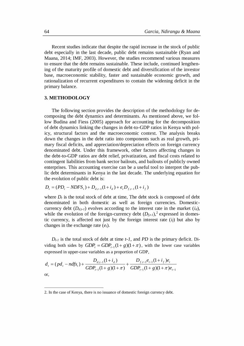
Garcia, Ndirangu & Maana
64
Recent studies indicate that despite the rapid increase in the stock of public
debt especially in the last decade, public debt remains sustainable (Ryan and
Maana, 2014; IMF, 2003). However, the studies recommend various measures
to ensure that the debt remains sustainable. These include, continued lengthen-
ing of the maturity profile of domestic debt and diversification of the investor
base, macroeconomic stability, faster and sustainable economic growth, and
rationalization of recurrent expenditures to contain the widening deficit in the
primary balance.
3. METHODOLOGY
The following section provides the description of the methodology for de-
composing the debt dynamics and determinants. As mentioned above, we fol-
low Budina and Fiess (2005) approach for accounting for the decomposition
of debt dynamics linking the changes in debt-to-GDP ratios in Kenya with pol-
icy, structural factors and the macroeconomic context. The analysis breaks
down the changes in the debt ratio into components such as real growth, pri-
mary fiscal deficits, and appreciation/depreciation effects on foreign currency
denominated debt. Under this framework, other factors affecting changes in
the debt-to-GDP ratios are debt relief, privatization, and fiscal costs related to
contingent liabilities from bank sector bailouts, and bailouts of publicly owned
enterprises. This accounting exercise can be a useful tool to interpret the pub-
lic debt determinants in Kenya in the last decade. The underlying equation for
the evolution of public debt is:
)1()1()( 1,1, ftftdtdttt iDeiDNDFSPDD
where Dt is the total stock of debt at time, The debt stock is composed of debt
denominated in both domestic as well as foreign currencies. Domestic-
currency debt (Dd,t-1) evolves according to the interest rate in the market (id),
while the evolution of the foreign-currency debt (Df,t-1),2 expressed in domes-
tic currency, is affected not just by the foreign interest rate (if) but also by
changes in the exchange rate (et).
Dt-1 is the total stock of debt at time t-1, and PD is the primary deficit. Di-
viding both sides by )1)(1(1 gGDPGDP tt , with the lower case variables
expressed in upper-case variables as a proportion of GDP,
11
11,
1
1,
)1)(1(
)1(
)1)(1(
)1()(
tt
tfttf
t
dtd
tttegGDP
eieD
gGDP
iDndfspdd
or,
2. In the case of Kenya, there is no issuance of domestic foreign currency debt.

Public debt dynamics in Kenya
65
)1)(1(
)1)(1(
)1)(1(
)1()( 1,1,
g
sid
g
idndfspdd
tf
tf
d
tdttt (1)
)1)(1(
)1)(1(
)1)(1(
)1()1()( 11
g
sid
g
idndfspdd
tf
t
d
tttt
)]1)(1()1)(1[()1)(1(
)( 1
tfd
t
ttt siig
dndfspdd
(2)
Define )1()1(ˆtfd siii as the average nominal interest rate on public
debt, and equation (2) can be rewritten as
]1ˆ[)1)(1(
)( 1
t
t
ttt sig
dndfspdd
, (3)
The average nominal interest rate, i , is calculated as ratio of interest payments
on debt divided by the previous period stock of public debt.
Subtracting 1td from both sides of equation (3) yields
111)1)(1(1)1)(1(
ˆ)(
t
t
ttttt dg
sd
g
gd
g
indfspdd
(4)
Based on the conversion of nominal change in exchange rate into real terms,
1
*)1)(1(
1
1 ts
RXR, after some algebra, it is possible to show that the nu-
merator of the last term in equation (4) is:
)1(*)1)(1(
1)1(
*1
1
RXRRXRst
(5)
Substituting (5) into (4) gives the basic accounting framework for public debt de-
composition:
g
d
RXR
RXR
i
g
dd
g
gndfspdd
t
t
tttt
1)1*)(1(
]*)1)(1(
)*(
1
1
ˆ[
1)1()(
1
1
1
(6)
where,
tD - total public debt, td = tD / tGDP
dtD - domestic public debt, dtd = dtD / tGDP
ftD - foreign public debt, ftd = te ftD / tGDP
tPD - primary deficit, tpd = tPD / tGDP
tNDFS - non-debt financing sources, ttt GDPNDFSndfs /

Garcia, Ndirangu & Maana
66
te – nominal exchange rate (domestic currency per U.S. dollar)
ts - changes in the nominal exchange rate: 1+ts =
te /1te , with
ts > 0 indicat-
ing nominal depreciation of the local currency
g – real GDP growth rate
π – domestic inflation (change in the domestic GDP deflator)
π* - U.S. inflation (change in U.S. GDP deflator)
di - nominal interest rate on domestic debt
fi - nominal interest rate on foreign debt
RXR – change in bilateral real exchange rate, with RXR > 0 indicating real
exchange rate appreciation defined as:
1
*)1)(1(
1
1 ts
RXR
α - the share of foreign currency denominated debt in total public debt
(1
1,
t
tf
d
d )
4. RESULTS
We provide results for both the ‘old’ and ‘rebased’ GDP series (Figures 6
and 7). The estimation based on the new rebased GDP series is limited as data
is available from 2006 only. The results do not vary much. From Figure 6, a
decline in debt-to-GDP ratio is observed during the period 2003-2007. This is
largely driven by the growth and revaluation effects. The high residuals in
2003 could be associated with a debt relief about this time. In 2000 and 2004,
Kenya rescheduled, under the Paris Club, debt arrears and flows effectively
receiving 50% debt relief in present value terms (GOK, 2007). There is also an
indication of tightening of fiscal policy during this period. The combined ef-
fects of primary surpluses, strong growth and revaluation effects with smaller
interest rate payments on debt and lower expenditure levels led to a reduction
of total Debt-to-GDP ratio during the period 2003-2007. After 2008-2011
smaller growth effects and revaluation effects (depreciation) along with an in-
creased since 2007 and have reached to over 3.5 % of the new rebased GDP.
Debt monetization has averaged about 3% during the study period.
During the period 2008-2014 period (Figure 7), smaller growth effects and
increases in the interest rates can be observed. While a looser fiscal policy
may have been in effect, a tightening of monetary policy to contain inflation-
ary pressures was taking place during the same period. The tightening of mon-
etary policy led to an increase in the cost of borrowing, and this brings up the
issue of policy coordination.

Public debt dynamics in Kenya
67
Figure 6. Kenya: Debt Dynamics, 2004-2014
Source: Authors’ calculations
Note: The interpretation of this chart is as follows. The colored segments of each column rep-
resent the contribution of each factor in our debt decomposition to the year on year change in the debt/GDP ratio. Items above the zero line contributed to an increase in the debt/GDP ratio,
while items below the zero line contribute to a reduction in the debt/GDP ratio. As an exam-
ple, a negative sign for Contribution from real GDP growth in a given year indicates that posi-
tive real GDP growth during that year contributed to a reduction in the debt/GDP ratio. On the
same token, a positive sign for the Contribution from real exchange rate changes indicates that
a real depreciation increased the debt/GDP ratio during that year.
Figure 7. Kenya: Debt Dynamics, 2007-2014
Source: Author’s Calculations
Garcia, Ndirangu & Maana
68
These findings are in line with those of Budina and Fiess (2005) who find
that in large reductions in debt to GDP, fiscal consolidation was a key compo-
nent of credible debt reduction. They also find that declines in debt ratios were
also determined by growth and appreciation effects. In this study, we find that
these factors were also key in lowering the debt ratio during the 2003-2007,
when the debt ratio declined from 64 to 42% of GDP. However, the exchange
rate appreciation need to be assessed further to ensure that the appreciation is
not the result of overvaluation3, or that may bring short term gains but have
long term impacts in terms of competitiveness. On the other hand, if the ap-
preciation is the result of productivity gains, the implications in terms of po-
tential output can contribute to further public debt reduction and reinforce the
growth effect. Although the currently available National accounts data do not
provide evidence of productivity growth above that of Kenya’s trading part-
ners, there could be under reporting and the on-going revisions will review the
true status.
Table 2 further summarizes the cumulative public debt decomposition and
tries to link changes in debt-to-GDP ratios to episodes of marked policy
change. During the period 2003-2005, Kenya public sector debt-to-GDP ratio
declined by about 4.5%. The main factors behind this decline were a combina-
tion of primary fiscal surpluses, economic growth and a substantial contribu-
tion from real exchange rate change. The only factors driving the debt ratio up
were interest payments and unaccounted factors. This period marked general
election in December 2002 and a change in government in January 2003.
With economic recovery during the period 2005-2007, Kenya managed to
reduce the public debt-to-GDP dropped by almost 19% during the period
2005-2008 A strong growth effect and appreciation of the shilling contributed
to this decline.
The public debt-to-GDP ratio took a turn in 2008-2011 driven mainly by
growth in primary deficits and interest payments. The ratio increased by 7.6
percentage points driven primary deficits and interest payments. Unlike other
periods, changes in real exchange rate contributed positively to the debt ratio.
This negative development can be linked to the post-election crisis in early
2008 and the global economic and financial crisis and the associated economic
3. In Ndirangu et.al (2014), the real exchange rate appreciation is found to be the main driver
of macroeconomic vulnerability in Kenya. A caveat is made that given a break in the real ex-
change rate may mean a new equilibrium level and not necessarily a misalignment. Mweiga
(2014) and Kiptui et al. (2014) observe that the shilling’s overvaluation is marginal at about
4%. However, this view is at variant with World Bank’s (2013) opinion that an overvalued
exchange rate is hurting the countries competitiveness. IMF (2014) reports similar findings.
While the IMF 2011 Article IV found Kenya’s real exchange rate to be broadly in line with
fundamentals, subsequent real appreciation has occurred at the same time as a sharp decline in
the terms of trade, which declined by some 18% from end-2010 to end-June 2014.

Public debt dynamics in Kenya
69
stimuli. The exchange rate crisis of 2011 in Kenya may be responsible for the
positive reevaluation effect. The period after the crisis (2011-2012), growth in
the debt-to-GDP ratio decelerated to about 1.5%. The appreciation of the shil-
ling once again contributed towards debt reduction. The debt-to-GDP ratio has
taken a turn in the most recent past. The ratio increased by 4.6% during the
period 2012-2014, with the contribution of the primary deficit recording the
highest rise. Primary deficit grew by 13 percentage points during this period.
Table 2. Cumulative public debt decomposition
2003-
2005
2005-
2008
2008-
2011
2011-
2012
2012-
2014
Percent of GDP
Change in public
sector debt -4.5 -19.2 7.6 1.5 4.6
Interest payments 7.1 9.0 8.9 5.0 8.6
Primary Deficit (- a
surplus) -3.0 2.8 10.9 6.2 13.0
Growth effect -8.3 -10.8 -6.3 -4.4 -6.9
Revaluation effect -5.1 -11.3 1.2 -3.4 -6.8
Seigniorage -2.2 -3.3 -3.5 -2.0 -2.5
Residual (other fac-
tors) 7.0 -5.6 -3.7 0.1 -0.8
Source: Authors computations
Although the primary fiscal balance is an imperfect measure of the fiscal
stance because it does not account for the quality or the durability of the fiscal
effort and its impact on growth, the rise in the debt ratio since 2007 may be of
concern. Although a recent analysis shows Kenya’s debt remains sustainable
and resilient to standard shocks, rising contingent liabilities are a fiscal risk
(IMF, 2014). The new subnational government level demands that fiscal disci-
pline will have to be observed by both the national and the county government
level to ensure long term fiscal sustainability. It is also of concern that the ex-
penditure increases have been due to increases in recurrent expenditures, even
though attempts to increase development expenditures have been made. Budi-
na and Fiess also note the strong link between quality of fiscal management
and strong efficient institutional arrangements that can aid to implement effec-
tive fiscal policy, manage liabilities and control and limit fiscal risk. And in
cases where institutional arrangements are not strong, countries have opted for
rule-based fiscal policies to establish fiscal credibility. Kenya adopted a budg-
et base and a revenue rule since 1997. Bova et.al (2014), however, shows that
these rules have not been very effective in reducing pro-cyclicality of fiscal
policy in Kenya. A pro-cyclical fiscal policy may inhibit growth during down-
turns and lead to increase public debt.
Garcia, Ndirangu & Maana
70
5. CONCLUSIONS
The increase in fiscal deficits and public debt highlights challenges in
maintaining fiscal discipline. The loose fiscal policy now may require the gov-
ernment to follow a fiscal tightening in the future in order to achieve a fiscal
deficit that is in line with the macro fiscal and debt sustainability framework.
The results of our debt dynamics analysis show that the expansionary fis-
cal policy that started since 2007 with increasing primary deficits along with
increased interest payments on public debt, mainly domestic debt, has led to
an erosion of the gains achieved in the reduction of the public debt ratio from
2003-2007, when a combination of primary fiscal surpluses and growth and
revaluation effects contributed to a drastic decline in total public debt.
Our results show that: (i) primary fiscal surpluses, real GDP growth and
reevaluation effects contributed to drastic decline debt-to-GDP during the
2003-2007; (ii) there was a shift in the contribution of the primary deficit and
the real exchange rate towards raising the aggregate debt ratio thereafter.
However, the reevaluation effect has pulled down debt since 2012; (iii) other
factors have followed a similar pattern: largely contributing to debt reduction
up to 2009 and to debt accumulation thereafter. There is need for further ex-
amination of the exchange rate appreciation to ensure that the appreciation is
the result of productivity gains and not due to undue overvaluation. Apprecia-
tion that comes from productivity gains can contribute to further debt reduc-
tion and reinforce the growth effect.
A rising debt-to-GDP ratio coupled with a pro-cyclical fiscal policy may
inhibit growth during downturns and increase public debt further, as it may
seem to be the case in the recent years. A commitment for responsible fiscal
and debt management will be critical to keep public debt in check, and ad-
justment policies that lead to productivity gains, along with better institutions
can lead to higher growth, higher savings and help lower the cost of borrow-
ing, reinforcing debt reducing public debt dynamics in Kenya.
REFERENCES
Bova, E., Carcenac, N., Guerguil, M. (2014) Fiscal Rules and the Procyclical-
ity of Fiscal Policy in the Developing World, IMF Working Paper, WP/14/22,
Washington, DC: IMF
Budina, N., Fiess, N., (2005) Public Debt and Its Determinants in Market Ac-
cess Countries, Washington, DC: The World Bank.

Public debt dynamics in Kenya
71
Daniel, J.A., Callen T., Terrones M., Debrun X., Allard C., (2003) Public Debt
in Emerging Markets: Is it too High? World Economic Outlook, Washington,
DC: IMF.
Das U.S., Papapioannou M., Pedras G., Ahmed F., Surti J. (2010) Managing
Public Debt and Its Financial Stability Implications, IMF Working Paper,
WP/10/280, Washington, DC: IMF.
GOK (2007) Public Debt Annual Report 2005/06, Nairobi: Debt Management
Department, Ministry of Finance Kenya.
IMF (2014) Kenya 2014 Article IV Consultation, IMF Country Report No.
14/302, October 2014, Washington, DC: IMF.
IMF (2003) Kenya: debt sustainability analysis, IMF Country Report No.
03/400, Washington, DC: IMF.
IMF/World Bank (2001) Handbook on development of government bonds
market, Washington, DC: IMF/World Bank.
Kiptui, M.C; Wambua, J. and Maturu, B. (2013) Determination of the Equilib-
rium Real Exchange Rate and its Misalignment in Kenya, KSMS Working Pa-
per, No. 2013/05, Nairobi: Kenya School of Monetary Studies.
Kumar, M., Baldacci,E., Schaechter, A., Caceres, A., Kim, D., Debrun, X.,
Escolano, J., Jonas, J., Karam, P., Yakadina, I., and Zymek, R. (2009) Fiscal
Rules – Anchoring Expectations for Sustainable Public Finances, Washington,
DC: IMF [https://www.imf.org/external/np/pp/eng/2009/121609.pdf].
Kumar, M. and Woo, J., (2010) Public Debt and Growth, IMF Working Paper,
WP/10/174, Washington, DC: IMF.
Merotra, A., Miyajima, K. and Villar, A. (2012) ”Development of domestic
government bond markets in EMEs and their implications,” in: Fiscal policy,
public debt and monetary policy in emerging market economies, BIS Papers,
No 67:31-50, Basel: Bank for International Settlements.
Mohanty, M., (2012) “Fiscal policy, public debt and monetary policy in
EMEs: an overview” in: Fiscal policy, public debt and monetary policy in
emerging market economies, BIS No. 67:1-9, Basel: Bank for International
Settlements.
Monthly Economic Review, Several Issues, Central Bank of Kenya.

Garcia, Ndirangu & Maana
72
Montoro, C., Takats, E., Yetman, J., et.al (2012). “Is Monetary Policy Con-
strained by Fiscal Policy?” in: Fiscal policy, public debt and monetary policy
in emerging market economies, BIS No. 67:11-30, Basel: Bank for Interna-
tional Settlements.
Mwega, F. (2014) Real Exchange Rate misalignment and implications for the
nominal Exchange Rate level in Kenya in 2012, Nairobi: Central Bank of
Kenya.
Ndirangu, L., Ndung’u, N., Garcia, C., Nyamongo, E., Gitau, C., (2014) “Ear-
ly Warning Index for Macroeconomic Vulnerability in Kenya,” Journal of
Economic and Financial Modelling, 2(1)24-36.
Nyamongo, E., Sichei, M and Mutai, N. (2010) The Monetary and Fiscal Pol-
icy Interactions in Kenya, Nairobi: Central Bank of Kenya.
Reinhart C. M, Rogoff, K., Savastano, M.A (2003) Debt Intolerance, NBER
Working Paper No. 9908.
Reinhart C. M., and Rogoff, K. (2010) Growth in a Time of Debt, NBER
Working Paper, No. 15639.
Republic of Kenya (2013) Annual Public Debt Management Report, Nairobi:
National Treasury.
Terry R., and Maana I. (2014) An Assessment of Kenya’s Public Debt Dynam-
ics and Sustainability, Working Paper, Nairobi: Central Bank of Kenya.
Tomasz J., and Kozinski, W. (2012). “A Framework for Fiscal Vulnerability
Assessment and Its Application to Poland,” in: Fiscal policy, public debt and
monetary policy in emerging market economies, BIS No. 67:285-294, Basel:
Bank for International Settlements..
World Bank (2013). Kenya Economic Update, June, Edition No. 8.
.

73
5 HOUSEHOLD INCOME INEQUALITY IN POLAND
FROM 2005 TO 2013 – A DECOMPOSITION OF
THE GINI COEFFICIENT BY INCOME SOURCES
Patrycja Graca-Gelert
Warsaw School of Economics
ABSTRACT
The aim of this paper is the empirical analysis of the Gini coefficient decomposition by
income sources in Poland from 2005 to 2013. The decomposition was used to assess the con-
tribution of individual income components to overall income inequality in Poland.
The empirical analysis was based on non-identifiable, individual household budget sur-
veys data collected by Poland’s Central Statistical Office. The method of decomposition by
income components applied in this study was the approach of Lerman and Yitzhaki (1985).
The study revealed that income from hired work contributed to the greatest extent to
overall income inequality in Poland during the analyzed period. At the same time this in-
come source showed an almost continuous growth in explaining income inequality, reaching
almost 68% at its peak in 2011. Apart from income from hired work, among all analyzed
income sources only social insurance benefits’ contribution to income disparities was
changing significantly in relative terms, dropping from about 20% to 12% between 2005 and
2013. Income from self-employment was explaining about 15% of income inequality in Po-
land during the analyzed period. The contribution of the rest of income sources to income
inequality was also relatively stable, though less significant. The only income category that
contributed negatively to income inequality was the component “other social benefits”.
The impact of a marginal change in income components on overall income inequality
was the largest in the case of income from hired work (positive effect) and social insurance
benefits (negative effect). A negative impact of a marginal change in specific income sources
upon inequality during the analyzed period was observed in the case of social insurance
benefits, other social benefits and other income (including gifts and alimonies).
1. INTRODUCTION
The decomposition of income inequality measures by income sources is
an important part of the analysis of income disparities, since it is helpful in
assessing the contribution of individual factor components to total income
inequality. The decomposition of income disparities may also be used as a
preliminary analysis of income inequality determinants.
Several years before Poland’s EU entry the debates on the economic and
social consequences of this decision gained momentum. Some people argued
that one of the effects of Poland’s accession into the EU would be a consid-

Graca-Gelert
74
erable increase in income inequality. More than a decade after the EU entry
this unfounded fear has not been supported by the official data, regardless of
their source. Another interesting issue is the structure of income inequality
and the question whether and to what extent it has changed after 2004.
The aim of this paper is the empirical analysis of the Gini coefficient de-
composition by factor components in Poland from 2005 to 2013 based on
non-identifiable, individual data from household budget surveys (Poland’s
Central Statistical Office). The following structure of the study was subordi-
nated to this aim. The first part presents the decomposition method used in
the empirical analysis and a short review of the empirical literature on the
Gini decomposition by factor components. The second part contains a de-
scription of the data used in this study. The results of the Gini decomposition
by income sources in Poland from 2005 to 2013 were presented in part three.
The analysis was preceded by an overview of income inequality trends in Po-
land during the analyzed period. The fourth part concludes.
2. ANALYTICAL FRAMEWORK
The research on the decomposition of inequality measures by income
sources gained momentum in the late 1970s and 1980s. Since then inequality
decomposition has been researched in depth, both in theoretical as well in
empirical terms1. The decomposition of the Gini coefficient – as one of the
most used inequality measures in analyses of income disparities – has also
been the subject of many studies to date.
The method of the Gini decomposition by income sources applied in this
empirical analysis was taken from the study of Lerman and Yitzhaki (1985).
This approach has been widely used in the literature on income inequality
decomposition (Table 1) and may be presented as follows (Lerman, Yitzhaki,
1985; Stark, Taylor, Yitzhaki, 1986). The point of departure is one of the
Gini coefficient formulas
(1) ,
where G0 represents the Gini coefficient of overall income and y0, μ0, F(y0)
denote income, mean income and the cumulative distribution of total income,
respectively. It is assumed that income may be divided into K income com-
ponents:
K
k kyy10 , where y1, …, yk are the income components. Thus,
we can write and transform equation (1) as follows:
1. A good review of the decomposition by income sources may be found for example in
Lerman (1999).

Household income inequality in Poland
75
(2)
(3)
(4) ,
where Sk denotes the share of component k in total income, Gk is the Gini co-
efficient corresponding to income component k and Rk is the Gini correlation
of component k with total income:
(5) .
The Gini correlation takes on values between -1 and 1, i.e. 1) if Rk is
equal to -1, then yk is a decreasing function of total income, 2) if Rk is equal
to 0, then yk and y0 are independent and 3) if Rk is equal to 1, then yk is an in-
creasing function of overall income.
Having determined the structure of inequality by income sources, the ef-
fect of a marginal change in individual income sources upon overall income
inequality may be calculated2. If we consider an exogenous change in each
person’s income from component k equal to ekyk, where ek is close to 1, then
(6)
(7)
The decomposition approach of Lerman and Yitzhaki (1985) is similar to
the method of Fei, Ranis and Kuo (1978), however, both methods differ in
their derivation and, somewhat, in their interpretation (Lerman, 1999). Yet
adding a part of the decomposition of Fei, Ranis and Kuo may facilitate and
be helpful in the interpretation of the contribution of individual income
sources to overall income. The components of their Gini decomposition are
the following (cf. Fei, Ranis, Kuo, 1978, pp. 47-48)
(8) ,
where is the so-called pseudo-Gini, which is simply the product of the
Gini correlation of income source k and the Gini coefficient corresponding to
income component k. The term “pseudo-Gini” is sometimes substituted by
“puppet Gini coefficient”, “centralizing rate of the income source k” or “con-
centration ratio of income source k” in the literature on income inequality
(Giorgi, 2011; Chen, Zhou, 2005). The difference between the pseudo-Gini
of income source k and the Gini coefficient corresponding to income compo-
nent k consists in the ordering of the income source k. Gk is calculated by the
order of source k itself, whereas is calculated for source k, when the rank-
2. A detailed derivation may be found in Stark, Taylor and Yitzhaki (1986).

Graca-Gelert
76
ing is based on total income. Thus both inequality measures are identical on-
ly if the ranking of income component k corresponds with the ranking of
overall income.
Comparing the values of the pseudo-Gini for each income source k and
the Gini coefficient for overall income allows us easily to assess directly the
impact of each income component on overall income inequality:
(1) if , then income source k is necessarily reducing overall income
inequality,
(2) if , then income source k enhances total income inequality,
(3) if , then the contribution of income source k to overall in-
come inequality is positive, although the source reduces income inequality to
some extent.
As has been mentioned, the literature yields numerous empirical studies
on the Gini coefficient decomposition by income components. Table 1 pre-
sents a review of selected empirical analyses. Most of them apply the de-
composition method of Lerman and Yitzhaki (1985).
Table 1. Selection of empirical studies on the Gini coefficient decomposi-
tion by factor components
Author/-s Year
of
public
Period of
analysis
Country
/countries
Decomposition
components
Method of analysis
Achdut L. 1996 1979-
1993
Israel Family head’s
earnings,
spouse’s earn-
ings, other’s
earnings, trans-
fer payments, other family
income, occupa-
tional pensions,
direct taxes
Gini coefficient de-
composition by in-
come sources (Ler-
man, Yitzhaki, 1985)
and subgroups, time-
series regression on macroeconomic vari-
ables
Araar A. 2006 2001 Cameroon Food expendi-
tures, non-food
expenditures
Gini coefficient de-
composition by ex-
penditure compo-
nents (Araar, 2006)
and subgroups; a de-
tailed theoretical
analysis of inequality
decomposition
Azam M., Shariff A.
2009 1993, 2005
Rural India Farm income, salaries, agricul-
tural wages,
non-agricultural
wages, income
Gini coefficient de-composition by in-
come sources (Ler-
man, Yitzhaki, 1985)
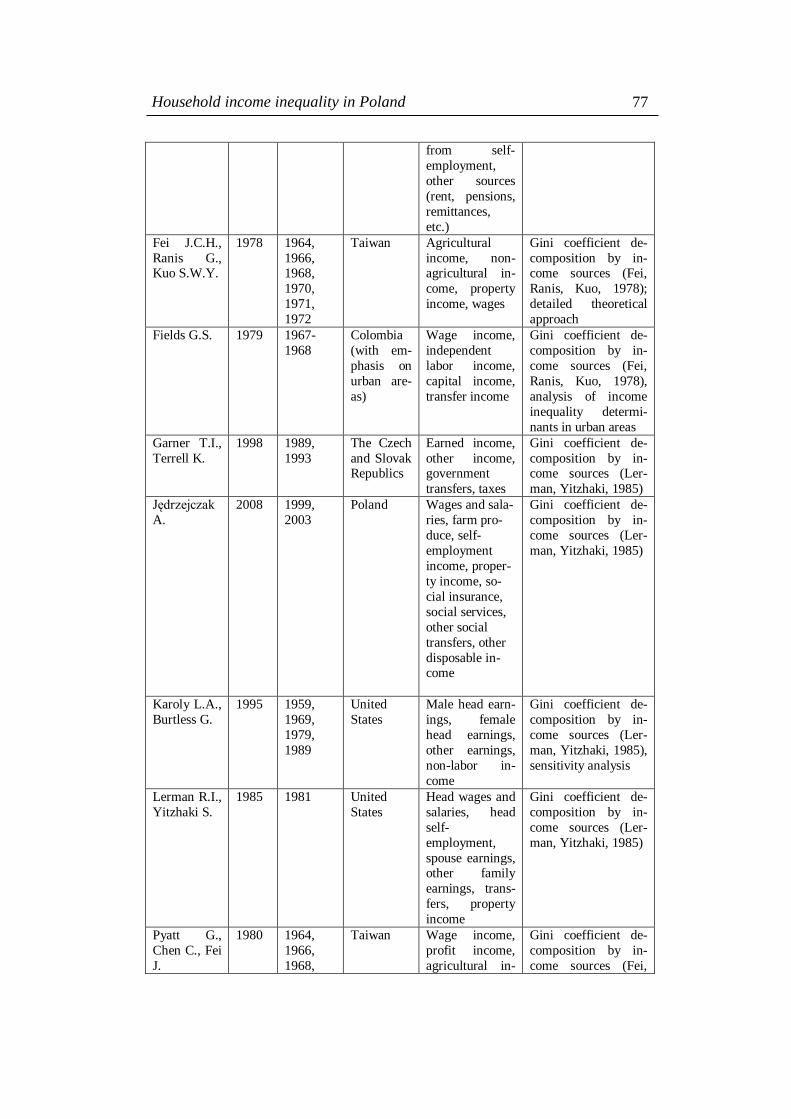
Household income inequality in Poland
77
from self-
employment,
other sources
(rent, pensions,
remittances,
etc.)
Fei J.C.H.,
Ranis G., Kuo S.W.Y.
1978 1964,
1966, 1968,
1970,
1971,
1972
Taiwan Agricultural
income, non-agricultural in-
come, property
income, wages
Gini coefficient de-
composition by in-come sources (Fei,
Ranis, Kuo, 1978);
detailed theoretical
approach
Fields G.S. 1979 1967-
1968
Colombia
(with em-
phasis on
urban are-
as)
Wage income,
independent
labor income,
capital income,
transfer income
Gini coefficient de-
composition by in-
come sources (Fei,
Ranis, Kuo, 1978),
analysis of income
inequality determi-
nants in urban areas
Garner T.I.,
Terrell K.
1998 1989,
1993
The Czech
and Slovak Republics
Earned income,
other income, government
transfers, taxes
Gini coefficient de-
composition by in-come sources (Ler-
man, Yitzhaki, 1985)
Jędrzejczak
A.
2008 1999,
2003
Poland Wages and sala-
ries, farm pro-
duce, self-
employment
income, proper-
ty income, so-
cial insurance,
social services,
other social
transfers, other
disposable in-come
Gini coefficient de-
composition by in-
come sources (Ler-
man, Yitzhaki, 1985)
Karoly L.A.,
Burtless G.
1995 1959,
1969,
1979,
1989
United
States
Male head earn-
ings, female
head earnings,
other earnings,
non-labor in-
come
Gini coefficient de-
composition by in-
come sources (Ler-
man, Yitzhaki, 1985),
sensitivity analysis
Lerman R.I.,
Yitzhaki S.
1985 1981 United
States
Head wages and
salaries, head
self-
employment,
spouse earnings, other family
earnings, trans-
fers, property
income
Gini coefficient de-
composition by in-
come sources (Ler-
man, Yitzhaki, 1985)
Pyatt G.,
Chen C., Fei
J.
1980 1964,
1966,
1968,
Taiwan Wage income,
profit income,
agricultural in-
Gini coefficient de-
composition by in-
come sources (Fei,

Graca-Gelert
78
1970,
1972,
1974,
1976
come, other
income
Ranis, Kuo, 1978);
detailed theoretical
analysis
Stark O.,
Taylor E.,
Yitzhaki S.
1986 1982 Two Mex-
ican vil-
lages in the
Pátzcuaro region of
the state of
Michoacán
Non-remittance
income, domes-
tic remittances,
United States-to-Mexico re-
mittances
Gini coefficient de-
composition by in-
come sources (Ler-
man, Yitzhaki, 1985); detailed theoretical
analysis
Wan G.H. 2001 1984-
1996
Rural
China
Wages, Farming
income, residual
income
Gini coefficient de-
composition by in-
come sources (meth-
od similar to the ap-
proach of Araar, 2006
and referring to Fei,
Ranis, Kuo, 1978)
Yao S. 1999 1990 Sichuan
province in
China
Farm income,
non-farm in-
come, time wages, non-time
wages, non-
wage income,
tax and transfer
Gini coefficient de-
composition by sub-
groups and income sources (method
based on the ap-
proach of Fei, Ranis,
Kuo, 1978)
Source: Own elaboration based on the cited studies.
3. DATA
The decomposition of the Gini coefficient by income sources in Poland
from 2005 to 2013 was based on non-identifiable, individual data from
household budget surveys (HBS) collected by Poland’s Central Statistical
Office (GUS)3. GUS conducts the HBS every year and the data are one of the
main sources of information on Poles’ expenditures, living conditions and
incomes. The surveys are based on a method of monthly rotation and on the
representative method. From 2005 to 2013 the HBS covered about 37.5 thou-
sand households, which is equivalent to slightly fewer than 110 thousand
persons (with the exception of 2005, when quite 35 thousand households
were surveyed).
Since 2005 no significant changes have occurred in the methodological
issues of HBS (cf. GUS, 2011, pp. 20-22; GUS, 2012, pp. 12-25; GUS, 2013,
pp. 13-26; GUS, 2014, pp. 14-28) with the exception of one change. A part
of the households selected by GUS refuse to participate in the survey, thus
3. The results of the empirical analysis presented in this study are the author’s own calcula-
tions based on data made available by GUS. GUS is not responsible for the conclusions con-
tained in this paper.

Household income inequality in Poland
79
the structure of the surveyed sample and the selected one differ in regard of
socio-economic traits. Therefore, the survey results have to be weighted with
the National Census data broken by the number of persons living in urban
and rural areas (GUS, 2014, p. 31) to allow for the generalization of the re-
sults to the whole population of households. In the case of the years 2005-
2012 the 2002 National Census was applied and for 2013 – the 2011 National
Census. However, apart from this exception, minor methodological changes
that occurred during the analyzed period did not have any noticeable impact
on the results of this empirical study. Thus, the HBS data and the obtained
results for individual years from 2005 to 2012 are comparable, with certain
attention on 2013.
For the purpose of this study income was defined as follows. Overall in-
come is the sum of income components that constitute available income ac-
cording to the definition of GUS. The following income sources were taken
into consideration:
1) income from hired work,
2) income from a private farm in agriculture,
3) income from self-employment (free profession),
4) income from property,
5) income from rental of a property or land,
6) social insurance benefits,
7) other social benefits,
8) other income (including gifts and alimonies).
Those income components that either revealed a substantial contribution
to overall income inequality or which contribution showed a considerable
change during the analyzed period were subject to a more in-depth analysis
in 2005, 2008, 2010 and 2013. These income sources were: I) income from
hired work and II) social insurance benefits. The first category of income
consists of: income from permanent hired work (domestic), income from
permanent hired work (foreign), compensation paid to retired or dismissed
persons, income from casual hired work (domestic), income from casual
hired work (foreign). The second category includes: old age pensions (do-
mestic), structural pensions, disability pensions (domestic), family pensions
(domestic), maternity benefits, other social insurance benefits, foreign social
insurance benefits (old age pensions, disability pensions). Some categories of
remittances were analyzed only from 2008 to 2013, because GUS did not
collect detailed data on foreign income sources before 2008.
In this study the household was chosen as unit of analysis. Household in-
come was adjusted using the modified equivalence scale, which assigns a
weight of 1 to the household head, 0.5 to each person aged 14 and above and
0.3 to each child.

Graca-Gelert
80
The income from a private farm in agriculture requires a comment. In
every year between 2005 and 2013 about 20-25% of households that record-
ed income from this source reported negative incomes in this category. Since
the calculation of the Gini coefficient requires income to be non-negative,
negative incomes from a private farm in agriculture were substituted by 0.
Thus, this adjustment might have had some impact on the real contribution of
incomes from this category on overall income.
The calculations were performed using Excel, Statistica 10 and DAD 4.6
– a software for distributive analysis (Jean-Yves Duclos, Abdelkrim Araar
and Carl Fortin, "DAD: A Software for Distributive Analysis/Analyse Dis-
tributive," MIMAP programme, International Development Research Centre,
Government of Canada, and CIRPÉE, Université Laval).
4. EMPIRICAL RESULTS
Before we analyze the components of the Gini coefficient decomposition
it is important to take a look at the trend of income inequality in Poland from
2005 to 2013. Figure 1 presents four time series of income inequality meas-
ured by the Gini coefficient. The differences between the data are clearly vis-
ible, especially if we compare, for example, the trends in inequality based on
Eurostat4 (EU-SILC) and GUS (HBS) data. We must bear in mind that the
differences in income inequality shown by individual data result from differ-
ent income distributions taken into account. In particular, the differences re-
sult from the choice of unit of analysis (EU-SILC – a person, HBS – a
household), the definition of income (EU-SILC – disposable income, HBS –
available income) and the applied equivalence scale (EU-SILC – the modi-
fied OECD equivalence scale, HBS – per capita income). In addition, a very
important problem are methodological issues related to the collection of data
(EU-SILC and HBS are two different databases), e.g. the EU-SILC are annu-
al data and the HBS are collected on a monthly basis.
Figure 1 shows that the changes in income inequality based on HBS data
and calculated according to the assumptions adopted in this empirical study
(PGG GINI) were not significant during the analyzed period. Income dispari-
ties were relatively stable from 2005 to 2013. Nonetheless, an interesting re-
search problem is the structure of income disparities and whether it changed
during the analyzed period and to what extent. The Gini coefficient decom-
position carried out below is aimed at answering this question.
4. To be precise, EU-SILC data are also collected by GUS.
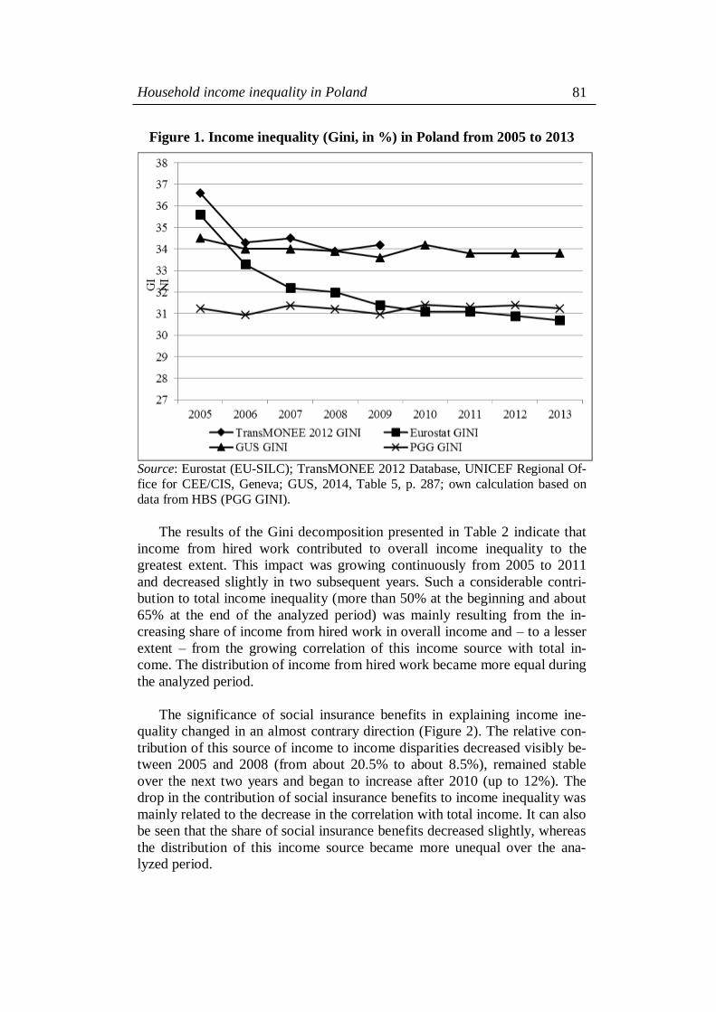
Household income inequality in Poland
81
Figure 1. Income inequality (Gini, in %) in Poland from 2005 to 2013
Source: Eurostat (EU-SILC); TransMONEE 2012 Database, UNICEF Regional Of-
fice for CEE/CIS, Geneva; GUS, 2014, Table 5, p. 287; own calculation based on
data from HBS (PGG GINI).
The results of the Gini decomposition presented in Table 2 indicate that
income from hired work contributed to overall income inequality to the
greatest extent. This impact was growing continuously from 2005 to 2011
and decreased slightly in two subsequent years. Such a considerable contri-
bution to total income inequality (more than 50% at the beginning and about
65% at the end of the analyzed period) was mainly resulting from the in-
creasing share of income from hired work in overall income and – to a lesser
extent – from the growing correlation of this income source with total in-
come. The distribution of income from hired work became more equal during
the analyzed period.
The significance of social insurance benefits in explaining income ine-
quality changed in an almost contrary direction (Figure 2). The relative con-
tribution of this source of income to income disparities decreased visibly be-
tween 2005 and 2008 (from about 20.5% to about 8.5%), remained stable
over the next two years and began to increase after 2010 (up to 12%). The
drop in the contribution of social insurance benefits to income inequality was
mainly related to the decrease in the correlation with total income. It can also
be seen that the share of social insurance benefits decreased slightly, whereas
the distribution of this income source became more unequal over the ana-
lyzed period.

Graca-Gelert
82
Since 2007 the second most important income source explaining income
inequality in Poland was income from self-employment. Its contribution to
overall income inequality was relatively stable throughout the analyzed peri-
od at about 15%. As can be seen in Table 2, the distribution of income from
self-employment was very unequal and highly correlated with overall in-
come. These two factors influencing income inequality were compensated by
a relatively low share of this income source in total income, although it was
rising slightly over almost the entire analyzed period.
Income from property and income from rental of a property or land were
contributing negatively to overall income inequality from 2005 to 2013. Both
categories of income are characterized by a very unequal distribution and a
high correlation with total income. Nevertheless these income sources were
explaining a marginal part of total income inequality as a consequence of
their very small share in overall income.
The contribution of other income (including gifts and alimonies) to in-
come inequality was decreasing from year to year during the analyzed period.
This income source was unequally distributed, however its correlation with
overall income was low, which explains why this income component was
reducing income inequality from 2005 to 2013. Nevertheless the share of
other income in overall income was decreasing, what resulted in a diminish-
ing contribution of this income source to total income inequality.
The income source that was necessarily (absolutely) reducing overall in-
come disparities during the period 2005-2013 were other social benefits,
which is shown by the negative value of the Gini correlation and thus the
pseudo-Gini. However, the share of other social benefits in total income
dropped by almost a half, which despite the accompanying rising inequality
of this income source limited its negative contribution to overall income ine-
quality, which was relatively stable during the analyzed period.
In the case of income from a private farm in agriculture, the contribution
to overall income inequality was somewhat changing during the period of
2005-2013, fluctuating between 5% and slightly above 7%. The share of
farm income in total income was relatively stable and inequality of this in-
come source was slightly rising. The Gini correlation was the most variable
term of the Gini decomposition of farm income.
As has been already mentioned, income from a private farm in agriculture
gives rise to some problems in interpreting its contribution to overall income
inequality, because this source of income was subject to the adjustment of
negative incomes. The issue of negative incomes in this category of income
source results probably from the fact that the HBS data are collected on a
monthly basis. Since income from a private farm in agriculture “is measured

Household income inequality in Poland
83
as a difference between the farm’s output (including natural consumption),
supplement connected with use of private farm in agriculture and current in-
vestment in the farming production and farm-related tax” (GUS, 2014, p. 33),
in some months income in this category may be negative. However, the cal-
culation of income inequality and the contribution of farm income to income
inequality would be probably more precise if income from this source was
calculated on an annual basis to avoid the bias related to negative income.
Table 2. Compositiona of income inequality in Poland – 2005-2013
Income
source Year Sk Gk Rk GkRk SkGkRk (SkGkRk)/G0 [(SkGkRk)/G0] – Sk
Income from
hired work
2005 0.4221 0.6780 0.6105 0.4139 0.1747 0.5592 0.1371
2006 0.4367 0.6599 0.6055 0.3996 0.1745 0.5640 0.1273
2007 0.4649 0.6386 0.6300 0.4023 0.1870 0.5959 0.1310
2008 0.4949 0.6233 0.6596 0.4112 0.2035 0.6518 0.1569
2009 0.4924 0.6284 0.6605 0.4150 0.2044 0.6596 0.1672
2010 0.4983 0.6270 0.6713 0.4209 0.2097 0.6677 0.1694
2011 0.5050 0.6251 0.6721 0.4201 0.2122 0.6776 0.1726
2012 0.5039 0.6263 0.6664 0.4173 0.2103 0.6698 0.1660
2013 0.4947 0.6274 0.6498 0.4077 0.2017 0.6453 0.1506
Income from
self-
employment
(free profes-
sion)
2005 0.0739 0.9519 0.6231 0.5931 0.0438 0.1402 0.0664
2006 0.0792 0.9526 0.6461 0.6155 0.0487 0.1575 0.0783
2007 0.0830 0.9494 0.6630 0.6295 0.0522 0.1664 0.0834
2008 0.0825 0.9465 0.6381 0.6040 0.0498 0.1596 0.0771
2009 0.0843 0.9434 0.6212 0.5860 0.0494 0.1595 0.0752
2010 0.0855 0.9407 0.6171 0.5805 0.0496 0.1579 0.0725
2011 0.0827 0.9415 0.6032 0.5679 0.0470 0.1500 0.0673
2012 0.0812 0.9426 0.5890 0.5552 0.0451 0.1436 0.0624
2013 0.0809 0.9427 0.6006 0.5662 0.0458 0.1465 0.0657
Income from
property
2005 0.0004 0.9995 0.8158 0.8154 0.0003 0.0010 0.0006
2006 0.0006 0.9995 0.8102 0.8099 0.0005 0.0016 0.0010
2007 0.0015 0.9995 0.9367 0.9362 0.0014 0.0045 0.0030
2008 0.0005 0.9996 0.8243 0.8239 0.0005 0.0014 0.0009
2009 0.0006 0.9994 0.8712 0.8707 0.0006 0.0018 0.0012
2010 0.0004 0.9997 0.8769 0.8767 0.0004 0.0012 0.0008
2011 0.0007 0.9996 0.8419 0.8416 0.0006 0.0019 0.0012
2012 0.0009 0.9998 0.8993 0.8992 0.0009 0.0027 0.0018
2013 0.0011 0.9996 0.8562 0.8559 0.0009 0.0029 0.0018
Income from
rental of a
property or
land
2005 0.0031 0.9956 0.5878 0.5852 0.0018 0.0059 0.0027
2006 0.0026 0.9965 0.6402 0.6379 0.0016 0.0053 0.0027
2007 0.0030 0.9962 0.6784 0.6758 0.0021 0.0065 0.0035

Graca-Gelert
84
2008 0.0033 0.9965 0.7252 0.7227 0.0024 0.0077 0.0044
2009 0.0029 0.9956 0.6328 0.6300 0.0018 0.0059 0.0030
2010 0.0036 0.9955 0.6901 0.6870 0.0025 0.0080 0.0043
2011 0.0038 0.9950 0.6658 0.6625 0.0025 0.0080 0.0042
2012 0.0040 0.9955 0.7416 0.7382 0.0029 0.0094 0.0054
2013 0.0040 0.9947 0.7261 0.7223 0.0029 0.0092 0.0052
Social insur-
ance benefits
2005 0.3396 0.6456 0.2934 0.1894 0.0643 0.2058 -0.1337
2006 0.3321 0.6468 0.2684 0.1736 0.0577 0.1863 -0.1457
2007 0.3062 0.6502 0.1863 0.1211 0.0371 0.1182 -0.1880
2008 0.2964 0.6507 0.1363 0.0887 0.0263 0.0842 -0.2122
2009 0.3042 0.6520 0.1530 0.0998 0.0304 0.0980 -0.2062
2010 0.2950 0.6582 0.1383 0.0910 0.0268 0.0855 -0.2095
2011 0.2969 0.6611 0.1508 0.0997 0.0296 0.0945 -0.2024
2012 0.2935 0.6685 0.1584 0.1059 0.0311 0.0990 -0.1945
2013 0.3004 0.6712 0.1866 0.1252 0.0376 0.1204 -0.1800
Other social
benefits
2005 0.0515 0.8217 -0.2276 -0.1870 -0.0096 -0.0308 -0.0823
2006 0.0451 0.8289 -0.2391 -0.1982 -0.0089 -0.0289 -0.0739
2007 0.0394 0.8373 -0.2555 -0.2139 -0.0084 -0.0269 -0.0663
2008 0.0299 0.8555 -0.2977 -0.2546 -0.0076 -0.0244 -0.0544
2009 0.0277 0.8598 -0.3172 -0.2727 -0.0076 -0.0244 -0.0522
2010 0.0283 0.8639 -0.3394 -0.2932 -0.0083 -0.0264 -0.0547
2011 0.0273 0.8683 -0.3570 -0.3100 -0.0085 -0.0270 -0.0543
2012 0.0283 0.8671 -0.3653 -0.3168 -0.0090 -0.0285 -0.0568
2013 0.0290 0.8742 -0.3676 -0.3214 -0.0093 -0.0298 -0.0588
Other in-
come (in-
cluding gifts
and alimo-
nies)
2005 0.0679 0.8590 0.3645 0.3131 0.0213 0.0681 0.0001
2006 0.0619 0.8668 0.3384 0.2933 0.0182 0.0587 -0.0032
2007 0.0570 0.8857 0.3895 0.3450 0.0196 0.0626 0.0057
2008 0.0510 0.8920 0.3720 0.3318 0.0169 0.0542 0.0032
2009 0.0503 0.8906 0.3311 0.2949 0.0148 0.0479 -0.0024
2010 0.0506 0.8963 0.3459 0.3100 0.0157 0.0499 -0.0007
2011 0.0483 0.8928 0.3140 0.2803 0.0135 0.0433 -0.0051
2012 0.0502 0.8856 0.3037 0.2690 0.0135 0.0430 -0.0072
2013 0.0479 0.8888 0.2324 0.2066 0.0099 0.0317 -0.0162
Income from
a private
farm in
agriculture
2005 0.0415 0.9556 0.3985 0.3808 0.0158 0.0506 0.0091
2006 0.0419 0.9577 0.4281 0.4100 0.0172 0.0555 0.0136
2007 0.0451 0.9654 0.5245 0.5064 0.0228 0.0727 0.0276
2008 0.0414 0.9684 0.5098 0.4937 0.0204 0.0654 0.0240
2009 0.0374 0.9662 0.4432 0.4282 0.0160 0.0517 0.0143
2010 0.0383 0.9697 0.4765 0.4621 0.0177 0.0563 0.0180
2011 0.0354 0.9719 0.4715 0.4583 0.0162 0.0517 0.0164

Household income inequality in Poland
85
2012 0.0380 0.9725 0.5177 0.5035 0.0191 0.0610 0.0230
2013 0.0422 0.9752 0.5608 0.5469 0.0231 0.0739 0.0317
Overall
income
2005 1 0.3125 1 0.3125 0.3125 1 0
2006 1 0.3094 1 0.3094 0.3094 1 0
2007 1 0.3138 1 0.3138 0.3138 1 0
2008 1 0.3122 1 0.3122 0.3122 1 0
2009 1 0.3098 1 0.3098 0.3098 1 0
2010 1 0.3141 1 0.3141 0.3141 1 0
2011 1 0.3131 1 0.3131 0.3131 1 0
2012 1 0.3139 1 0.3139 0.3139 1 0
2013 1 0.3125 1 0.3125 0.3125 1 0
Note: a Sk – the share of component k in total income, Gk – the Gini coefficient cor-
responding to income component k, Rk – the Gini correlation of component k with
total income, GkRk – the pseudo-Gini, SkGkRk – the absolute contribution of income
source k to overall income inequality, (SkGkRk)/G0 – the relative contribution of in-come source k to overall income inequality, {[(SkGkRk)/G0] – Sk} – the effect of a
marginal percentage change in income source k upon overall income inequality.
Source: Own calculation based on HBS data.
The last column of Table 2 presents the effect of a small percentage
change in individual income sources upon overall income inequality. As can
be seen, a marginal change in three categories of income – social insurance
benefits, other social benefits and other income – had the effect of reducing
total income inequality during the analyzed period. The largest response to a
marginal percentage change in income source k upon overall income inequal-
ity was recorded in the case of income from hired work (a positive impact of
about 0.13-0.17%) and social insurance benefits (a negative impact of about
0.13-0.21%). The effect of a marginal percentage change of income from
property and income from rental of a property or land upon total income ine-
quality was very small, although it was increasing for each income source.
An unexpectedly small marginal effect upon overall income inequality was
observed in the case of income from a private farm in agriculture, however,
as it has already been pointed out this income component has to be treated
with caution.
Figure 2 shows that income from hired work explained overall income to
the greatest extent and that the contribution of both income from hired work
and social insurance benefits to inequality changed most significantly during
the analyzed period. Therefore these income sources were subject to a more
detailed analysis, i.e. these income sources were analyzed on a more dis-
aggregated level. The main results of the Gini decomposition (relative con-
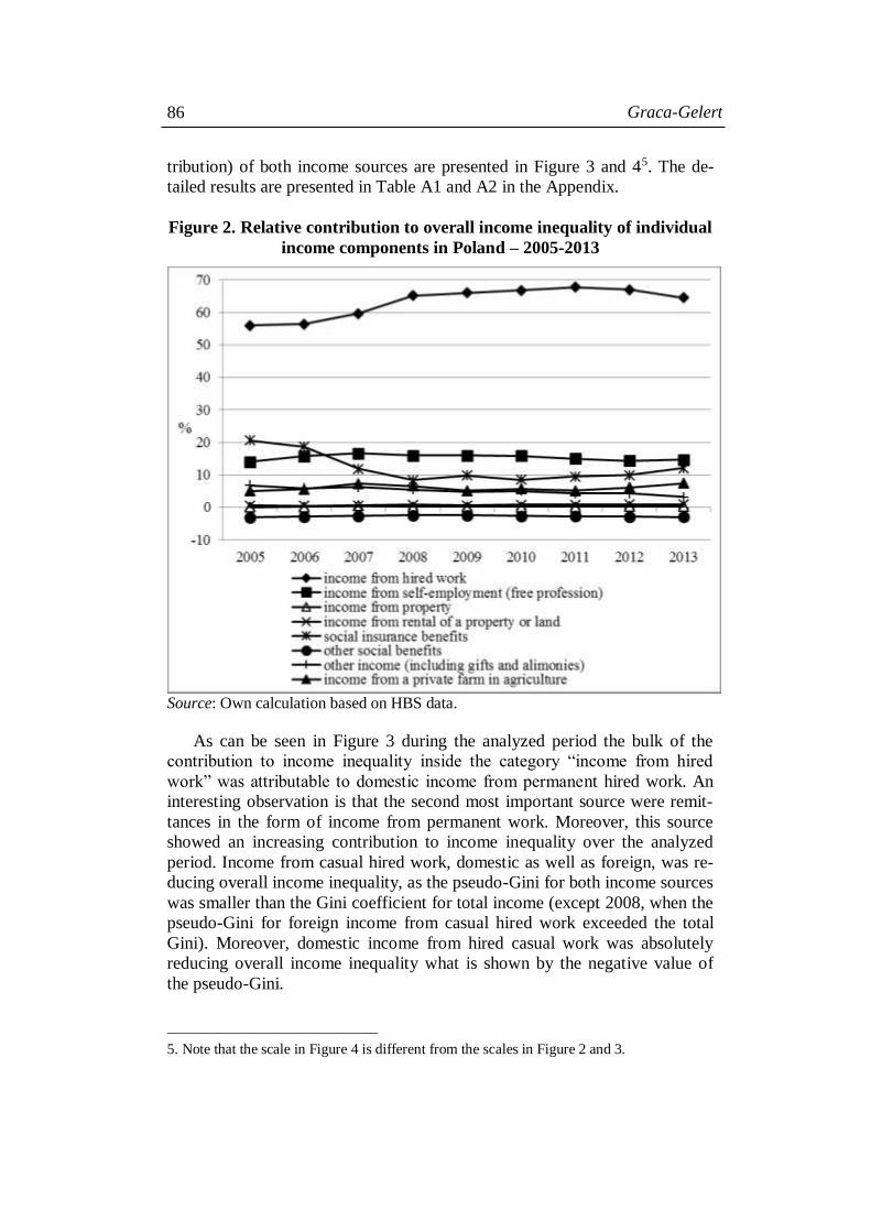
Graca-Gelert
86
tribution) of both income sources are presented in Figure 3 and 45. The de-
tailed results are presented in Table A1 and A2 in the Appendix.
Figure 2. Relative contribution to overall income inequality of individual
income components in Poland – 2005-2013
Source: Own calculation based on HBS data.
As can be seen in Figure 3 during the analyzed period the bulk of the
contribution to income inequality inside the category “income from hired
work” was attributable to domestic income from permanent hired work. An
interesting observation is that the second most important source were remit-
tances in the form of income from permanent work. Moreover, this source
showed an increasing contribution to income inequality over the analyzed
period. Income from casual hired work, domestic as well as foreign, was re-
ducing overall income inequality, as the pseudo-Gini for both income sources
was smaller than the Gini coefficient for total income (except 2008, when the
pseudo-Gini for foreign income from casual hired work exceeded the total
Gini). Moreover, domestic income from hired casual work was absolutely
reducing overall income inequality what is shown by the negative value of
the pseudo-Gini.
5. Note that the scale in Figure 4 is different from the scales in Figure 2 and 3.

Household income inequality in Poland
87
Figure 3. Relative contribution to overall income inequality of the com-
ponents of income from hired work
Source: Own calculation based on HBS data.
As regards social insurance benefits, there is also one dominant income
category contributing to overall income inequality – similarly to income from
hired work. As can be seen in Figure 4 domestic old age pensions explained
the bulk of overall income among all components of social insurance benefits
during the analyzed period. The second most important income source in this
regard were domestic disability pensions, that were necessarily reducing total
income inequality in 2005, 2008, 2010 and 2013. Other income sources
played a significantly smaller role in explaining overall income inequality.
An interesting observation is that other social insurance benefits and foreign
social insurance benefits were enhancing total income inequality, although
this impact was marginal because of their very small share in overall income.

Graca-Gelert
88
Figure 4. Relative contribution to overall income inequality of the com-
ponents of social insurance benefits
Source: Own calculation based on HBS data.
5. CONCLUSIONS
The Gini coefficient decomposition by income components carried out in
this study revealed that income from hired work was explaining overall in-
come inequality in Poland to the greatest extent among all income sources
during the period 2005-2013. The contribution of income from hired work to
total income inequality increased by 9 percentage points between 2005 and
2013, reaching almost 68% at its peak in 2011. On the other hand, the contri-
bution of social insurance benefits to overall income inequality was decreas-
ing during almost the entire analyzed period, starting to increase slightly in
the last three years. The rest of income sources did not show such great vari-
ability in explaining total income inequality. The income components that
were distributed most unequally and were highly correlated with total income
– income from property and income from rental of a property or land – had a
marginal contribution to overall income inequality because of their very
small share in total income. Other social benefits revealed an absolutely re-
ducing impact on total income inequality. However, their share in overall in-
come dropped by almost a half, which resulted in a decrease of the contribu-

Household income inequality in Poland
89
tion of this income source to overall income inequality. The importance of
other income decreased between 2005 and 2013.
Overall, the Gini decomposition results obtained in this empirical study are
not very surprising regarding the structure of income ineq
uality. For example, in developed countries income from hired work usually
explains the bulk of overall income disparities, whereas social benefits as e.g.
unemployment benefits or housing subsidies contribute to a reduction in in-
come inequality.
As L. Achdut emphasizes in the comment on the chapter of R.I. Lerman
(1999), the decomposition of income inequality by income sources is only
one way to explain trends in income inequality. A useful extension of this
analysis would be the decomposition of income inequality by subgroups or a
time series model explaining the relationship between income inequality
(components) and its potential determinants. Such a comprehensive analysis
would enable to identify the main factors influencing inequality and their
change over time. In addition, this empirical study could be extended by sev-
eral years. However, there appears a problem of data comparability, since
significant methodological changes occurred in HBS in the years previous to
2005.
It has to be emphasized that the assumptions adopted in this empirical
study determine the obtained results and its interpretation. These assumptions
concern mainly the unit of analysis, the definition of income and the equiva-
lence scale. Thus a very important remark is that the obtained results have to
be interpreted carefully, especially because any modification in the assump-
tions may change the results. As in most of the literature of income inequali-
ty, the trends and relative relations are what can be determined with greater
certainty and should rather be assessed in contrast to absolute values.
REFERENCES
Journal articles
Achdut, L. (1996) “Income inequality, income composition and macroeco-
nomic trends: Israel, 1979-1993”, Economica, 63(250):S1-S27.
Fei, J.C.H., Ranis, G., Kuo, S.W.Y. (1978) “Growth and the family distribu-
tion of income by factor components”, The Quarterly Journal of Economics,
92(1):17-53.
Fields, G.S. (1979) “Income inequality in urban Colombia: A decomposition
analysis”, Review of Income and Wealth, 25(3):327-341.

Graca-Gelert
90
Garner, T.I., Terrell, K. (1998) “A Gini decomposition analysis of inequality
in the Czech and Slovak Republics during the transition”, Economics of
Transition, 6(1):23-46.
Jędrzejczak, A. (2008) “Decomposition of the Gini index by sources of in-
come”, International Advances in Economic Research, 14(4):441-447.
Karoly, L.A., Burtless, G. (1995) “Demographic change, rising earnings ine-
quality, and the distribution of personal well-being, 1959-1989”, Demogra-
phy, 32(3):379-405.
Lerman, R.I., Yitzhaki, S. (1985) “Income inequality effects by income
source: a new approach and applications to the United States”, The Review of
Economics and Statistics, 67(1):151-156.
Pyatt, G., Chen, C., Fei, J. (1980) “The distribution of income by factor com-
ponents”, The Quarterly Journal of Economics, 95(3):451-473.
Rao, V.M. (1969) “Two decompositions of concentration ratio”, Journal of
the Royal Statistical Society, 132(3):418-425.
Stark, O., Taylor, E., Yitzhaki, S. (1986) “Remittances and inequality”, The
Economic Journal, 96(383):722-740.
Wan, G.H. (2001) “Changes in regional inequality in rural China: decompos-
ing the Gini index by income sources”, Australian Journal of Agricultural
and Resource Economics, 45(3):361-381.
Yao, S. (1999) “On the decomposition of Gini coefficients by population
class and income source: a spreadsheet approach and application”, Applied
Economics, 31(10):1249-1264.
Non-journal articles
Araar, A. (2006) “On the decomposition of the Gini coefficient: An exact
approach, with an illustration using Cameroonian data”, Cahier de recherché,
Working Paper, nr 06-02.
Azam, M., Shariff, A. (2009) “Changes in income inequality in rural India:
decomposing the Gini by income sources”, IZA and International Food Poli-
cy Research Institute.

Household income inequality in Poland
91
Books
Chen, Z., Zhou, Y. (2005) “Income distribution during system reform and
economic development in China: The status and trend of income inequality
of Chinese residents”, Nova Publishers.
GUS (2011) Metodologia badania budżetów gospodarstw domowych,
Warszawa: GUS, Departament Warunków Życia.
GUS (2012) Budżety Gospodarstw Domowych w 2011 r., Warszawa: GUS.
GUS (2013) Budżety Gospodarstw Domowych w 2012 r., Warszawa: GUS.
GUS (2014) Budżety Gospodarstw Domowych w 2013 r., Warszawa: GUS.
Milanovic, B. (1998) Income, inequality, and poverty during the transition
from planned to market economy, Washington, DC: World Bank, Regional
and Sectoral Studies.
Book chapter
Giorgi, G.M. (2011) “The Gini inequality index decomposition: An evolu-
tionary study”, in: J. Deutsch, J. Silber (eds) The measurement of individual
well-being and group inequalities: Essays in memory of Z.M. Berrebi, pp.
185-218, London: Routledge.
Lerman, R.I. (1999) “How do income sources affect income inequality?”
(with a comment by L. Achdut), in: J. Silber (ed) Handbook of income ine-
quality measurement, pp. 341-362, Kluwer Academic Publishers.

Graca-Gelert
92
APPENDIX
Table A1. Compositiona of income inequality – income from hired workb
Income source Year Sk Gk Rk GkRk SkGkRk (SkGkRk)/G0 [(SkGkRk)/G0] – Sk
Overall income
– income from
hired work
2005 0.5779 0.4847 0.4917 0.2383 0.1377 0.4408 -0.1371
2008 0.5051 0.5341 0.4030 0.2152 0.1087 0.3482 -0.1569
2010 0.5017 0.5288 0.3935 0.2081 0.1044 0.3323 -0.1694
2013 0.5053 0.5410 0.4054 0.2194 0.1109 0.3547 -0.1506
Income from
permanent
hired work,
domestic
2005 0.4074 0.6901 0.6158 0.4250 0.1731 0.5541 0.1467
2008 0.4716 0.6375 0.6507 0.4148 0.1956 0.6267 0.1550
2010 0.4792 0.6396 0.6659 0.4259 0.2041 0.6496 0.1704
2013 0.4732 0.6413 0.6431 0.4124 0.1951 0.6244 0.1512
Income from
permanent
hired work,
foreign
2005 . . . . . . .
2008 0.0106 0.9912 0.4493 0.4453 0.0047 0.0151 0.0045
2010 0.0109 0.9911 0.4381 0.4342 0.0047 0.0150 0.0042
2013 0.0147 0.9889 0.4494 0.4445 0.0065 0.0209 0.0062
Compensation
paid to retired
or dismissed
persons
2005 0.0014 0.9999 0.9712 0.9711 0.0014 0.0044 0.0030
2008 0.0012 0.9998 0.9606 0.9604 0.0012 0.0037 0.0025
2010 0.0002 0.9999 0.7587 0.7586 0.0002 0.0005 0.0003
2013 0.0002 0.9999 0.7601 0.7600 0.0002 0.0006 0.0003
Income from
casual hired
work, domestic
2005 0.0133 0.9703 0.0176 0.0171 0.0002 0.0007 -0.0126
2008 0.0097 0.9799 0.1214 0.1190 0.0012 0.0037 -0.0060
2010 0.0074 0.9835 0.0906 0.0891 0.0007 0.0021 -0.0053
2013 0.0059 0.9848 -0.0423 -0.0417 -0.0002 -0.0008 -0.0066
Income from
casual hired
work, foreign
2005 . . . . . . .
2008 0.0017 0.9986 0.4789 0.4783 0.0008 0.0026 0.0009
2010 0.0006 0.9991 0.2271 0.2269 0.0001 0.0005 -0.0002
2013 0.0006 0.9991 0.0836 0.0835 0.0001 0.0002 -0.0005
Note: a Sk – the share of component k in total income, Gk – the Gini coefficient cor-
responding to income component k, Rk – the Gini correlation of component k with
total income, GkRk – the pseudo-Gini, SkGkRk – the absolute contribution of income source k to overall income inequality, (SkGkRk)/G0 – the relative contribution of in-
come source k to overall income inequality, {[(SkGkRk)/G0] – Sk} – the effect of a
marginal change in income source k upon overall income inequality. b Missing data are marked with a dot.
Source: Own calculation based on HBS data.

Household income inequality in Poland
93
Table A2. Compositiona of income inequality – social insurance benefitsb
Income source Year Sk Gk Rk GkRk SkGkRk (SkGkRk)/G0 [(SkGkRk)/G0] – Sk
Overall income
– social insur-
ance benefits
2005 0.6597 0.5428 0.6918 0.3755 0.2477 0.7920 0.1323
2008 0.7036 0.5299 0.7669 0.4064 0.2859 0.9158 0.2122
2010 0.7057 0.5325 0.7650 0.4074 0.2875 0.9144 0.2087
2013 0.6996 0.5305 0.7406 0.3929 0.2749 0.8796 0.1800
Old age
pensions,
domestic
2005 0.2432 0.7603 0.3457 0.2628 0.0639 0.2044 -0.0388
2008 0.2304 0.7393 0.1800 0.1331 0.0307 0.0982 -0.1322
2010 0.2328 0.7402 0.1824 0.1350 0.0314 0.1000 -0.1328
2013 0.2374 0.7505 0.2291 0.1720 0.0408 0.1306 -0.1068
Structural
pensions
2005 . . . . . . .
2008 0.0017 0.9971 0.0156 0.0155 0.0000 0.0001 -0.0016
2010 0.0020 0.9965 0.0047 0.0047 0.0000 0.0000 -0.0020
2013 0.0019 0.9965 -0.0027 -0.0027 0.0000 0.0000 -0.0019
Disability
pensions,
domestic
2005 0.0528 0.8921 -0.1013 -0.0904 -0.0048 -0.0152 -0.0680
2008 0.0312 0.9219 -0.1673 -0.1542 -0.0048 -0.0154 -0.0466
2010 0.0262 0.9317 -0.1956 -0.1823 -0.0048 -0.0152 -0.0414
2013 0.0250 0.9384 -0.1824 -0.1711 -0.0043 -0.0137 -0.0387
Family
pensions,
domestic
2005 0.0408 0.9489 0.0892 0.0847 0.0035 0.0110 -0.0297
2008 0.0304 0.9556 -0.0324 -0.0310 -0.0009 -0.0030 -0.0334
2010 0.0315 0.9560 -0.0223 -0.0214 -0.0007 -0.0021 -0.0336
2013 0.0320 0.9562 -0.0401 -0.0383 -0.0012 -0.0039 -0.0359
Maternity
benefits
2005 0.0008 0.9986 0.6760 0.6750 0.0005 0.0017 0.0009
2008 0.0008 0.9982 0.3782 0.3775 0.0003 0.0010 0.0002
2010 0.0000 1.0000 -0.5713 -0.5713 0.0000 0.0000 0.0000
2013 0.0018 0.9971 0.4597 0.4584 0.0008 0.0026 0.0008
Other social
insurance
benefits
2005 0.0025 0.9977 0.6673 0.6657 0.0017 0.0053 0.0028
2008 0.0012 0.9990 0.6099 0.6093 0.0007 0.0024 0.0012
2010 0.0009 0.9989 0.4361 0.4357 0.0004 0.0013 0.0004
2013 0.0012 0.9990 0.5556 0.5550 0.0007 0.0021 0.0009
Social insur-
ance benefits
(old age pen-
sions, disability
pensions),
foreign
2005 0.0003 0.9995 0.7937 0.7933 0.0003 0.0009 0.0005
2008 0.0007 0.9994 0.4302 0.4299 0.0003 0.0010 0.0003
2010 0.0008 0.9994 0.6434 0.6430 0.0005 0.0016 0.0008
2013 0.0011 0.9995 0.7490 0.7486 0.0009 0.0027 0.0016
Note: a and b (see Table A1).
Source: Own calculation based on HBS data.

94
6 ANALYSIS OF THE RELATIONSHIP
BETWEEN PROFITABILITY AND DIVIDEND POLICY
OF BANKS ON THE GHANA STOCK EXCHANGE
John Kwaku Mensah Mawutor
Coordinator School of Graduate Studies (SOGS)
University of Professional Studies, Accra. Ghana
P.O. Box LG 149, Legon: Tel: 233243287242/
Email: [email protected] / [email protected]
Embele Kemebradikemor
Wisconsin International University College, Ghana
Box LG 751, Legon-Accra / Email: [email protected]
ABSTRACT
The relationship between dividends and earnings has long been a controversy to analyst
and investors. In view of this phenomenon, dividend policy still remains an unresolved issue in
contemporary corporate governance. This quantitative study, investigates the relationship
between profitability and dividend policy of banks listed on the Ghana Stock Exchange (GSE). Using a correlation analysis to test the relationship between profitability and dividend policy,
the (expected) result is that profitability and dividend policy are significantly related. Thus,
when the banks make profits they tend to pay out dividends. However, the study also shows
through a regression model that banks listed on the Ghana stock exchange employ a dividend
policy that is not solely influenced by profitability. There are also other factors, which ac-
count for the dividend policy that banks adopt. These other factors include liquidity, growth,
other investments, control, legal requirements, shareholders desires, size of the firm and other
management decisions.
Key words: Dividend, Investors, Policy, Listed Banks, Growth, Stock Exchange, Shareholders
JEL Code: A12
1. INTRODUCTION
The relationship between dividends and earnings has long been a contro-
versy to analyst and investors (Farsio, Amanda, & Justin, 2004). In view of the
numerous studies, dividend policy still remains an unsolved issue in contem-
porary corporate governance. According to Ajanthan (2013), the determinant
of dividend paid-out is a firm’s profitability. However, the percentage of divi-
dend paid out of the profit declared by most firms fall below stakeholders’ ex-
pectations. Enyan (2009), stated that some firms pay low or no dividend be-
cause management is optimistic about the firm’s future and wishes to increase
retain earnings for future expansion. Other firms might finance capital ex-

Dividend policy of banks on the Ghana stock exchange
95
penditure by borrowing largely from other sources which will release cash for
dividend payout. In view of these, managements are in a dilemma as to the
amount of profit to distribute as dividend.
Until recently, most banks have been reported to make huge profits, de-
clared dividends, thus making them attractive to stakeholders. Also, there are
some banks that declare little or no dividend despite profit or loss made
(Yekwe, 2011). This has brought about an objectionable question on the divi-
dend policy adopted by firms.
Since dividends are part of profit paid to shareholders as a return on their
investment, the questions therefore asked are; is there any significant relation-
ship between profitability and dividend policy? Is it that directors’ pay divi-
dend to impress shareholders thus making them the attraction of most inves-
tors? Or do managers pay low or no dividend just for retention of profit for
future expansion. From the aforementioned questions regarding dividend poli-
cy, there has arisen the need to investigate dividend policy in relation to prof-
itability hence this study seeks to analyze the relationship between profitabil-
ity and dividend policy of banks on the Ghana stock exchange. In this regard,
the main objective of this study is to investigate the nature and form of rela-
tionship between profitability and dividend policy of banks listed on the Gha-
na stock exchange. Specifically the study established the relationship between
profitability and dividend policy of banks listed on the Ghana stock exchange,
analyzed the extent of the relationship between profitability and dividend poli-
cy of banks listed on the Ghana stock exchange and identified the major fac-
tors influencing the dividend policy of banks listed on the Ghana stock ex-
change.
2. LITERATURE REVIEW
A number of studies have been conducted in the area of dividend pay-out
and profitability however; there are few studies in the establishment of rela-
tionship between profitability and dividend policies in the Ghana Stock ex-
change. The significance of this study is to reveal the relationship between
dividend policies and identify the factors that underline the payment of divi-
dends. In this regard, the study reviewed the conceptual framework underlin-
ing profitability and dividend policies. Dividend theories such as Litner
(1956), Gordon (1959), dividend relevance; Modigliani and Miller’s (1961),
dividend irrelevance theory and their tax preference theories were reviewed.
The dividend relevant theory advanced by Litner (1956) and Gordon
(1959), argued that investors prefer dividends to capital gains due to their cer-
tainty. They described the theory as “bird-in-hand” argument and means that
investors will prefer to receive a certain dividend payment now rather than
leaving the equivalent amount in an investment whose future is uncertain.

96 Mawutor & Kemebradikemor
Current dividends on this analysis represent a more reliable return than
future capital gains. They argued that dividend policy plays a vital role in de-
termining a share value of a firm since dividends are preferred to capital gains
by investors. Firms that pay low dividend may experience a fall in investment
and shareholders may shift to firms that offer dividend payment in a more lib-
eral manner.
In contrast, Litner’s (1956) and Gordon’s (1959) theory of dividend rele-
vance was criticized giving rise to the dividend irrelevance theory originated
with a paper published by Modigliani & Miller in 1961. They argued that
share valuation is a function of the level of corporate earnings, which reflects
a firm’s investment policy rather than a function of the proportion of a firm’s
earnings that are paid out as dividend. They further argued that the investment
decisions responsible for a firm’s future profitability are the only determinant
of its market value. For Modigliani & Miller 1961, share valuation is inde-
pendent of the level of dividend policy paid by a firm. Modigliani & Miller
(1961), observed that the investors who are rational are indifferent as to re-
ceiving dividend or capital gains on their shares as they make choices that
maximize their utility. What matters as from the perspective of shareholders
utility is that a firm maximizes its market value by adopting an optimal in-
vestment policy. This policy would enable the firm invest in projects that will
yield a net positive value and hence maximize the net present value of the firm
as a whole. By so doing, the firm may generate some internal fund as a result
of investing in projects that yield a positive net present value. These internal
funds will be retained and when surplus comes, they can be paid out as divi-
dend. This means that for Modigliani & Miller (1961), dividends are residual
payment if no dividends are paid because all earning have been consumed by
the firm’s optimum investment schedule. The market value of the firm will
increase to reflect the expected future dividend payment or increasing share
price resulting from investment returns.
However, the Modigliani and Miller (1961) dividend irrelevance theory
has been criticized since the assumptions do not apply to an imperfect market.
Enyan (2009), in his study stated that imperfect capital market such as Ghana
stock exchange companies incur floatation cost in raising additional cost and
shareholders incur cost when selling or buying shares. In Ghana, firms pay
brokerage fees or underwriting cost when issuing new shares. Again, investors
pay income tax in the dividend income they receive and dividend in Ghana is
subject to 8% (Ghana Tax Guide 2012) withholding tax while capital gains are
exempted from taxes. Furthermore, the insiders have more access to infor-
mation than the outsides, thus the market does not fully reflect all available
information. Clearly, these shows that dividend policy has a tremendous effect
on share price valuation in an imperfect market like the Ghana stock ex-
change.

Dividend policy of banks on the Ghana stock exchange
97
3. RELATED STUDIES
Many researchers have tried to uncover issues regarding the dividend
puzzle and determinants of dividend policy but we still don’t have an accepta-
ble explanation for the observed dividend behavior of firms (Brealey & Myers
2005). Dividend policy has been analyzed for many decades but no universal-
ly accepted explanation for firms observed dividend behavior has been estab-
lished (Samuel & Edward 2011). It has been a long mystery in corporate fi-
nance.
Enyan (2009) in his study examined the determinants of dividend payout
ratio of firms listed on the Ghana stock exchange for a six year period. He
found out that there is a positive relationship between dividend payout and
earnings per share, current ratio, and market capitalization. The result showed
that profitable firms tend to pay high dividend. His study further showed a
negative association between dividend payout and retained earnings, price to
book and debt to equity ratio, hence dividend relevance in firms.
Amindu (2007), carried out a study to examine corporate dividend poli-
cies of publicly traded companies in Ghana stock exchange for an eight year
period to determine whether dividend policy influences firms’ performance.
He found that dividend policy affects firms’ performance especially the profit-
ability, measured by returned on asset. The result of his study showed a posi-
tive relationship between return on asset, dividend policy and growth in sales.
This proves that when a firm has a policy to pay dividend, its profitability is
influenced. The result also showed statistically significant relationship be-
tween profitability and dividend payout ratio and also the study supports the
relevant theory that dividend policy is relevant to the performance of firms.
4. PROFITABILITY OF FIRMS
Profitability is one of the major goals of all business firms. Without prof-
itability it is difficult to anticipate the survival of a business in the long run as
profit ensures a business survival (Ross, 2004). Profitability can simply be re-
ferred to as the ability to make profit from all the business activities of an or-
ganization, company, firm, or an enterprise (Rustagi, 2012). It shows how ef-
ficiently the management can make profit by using all the resources available
in them. Thus, "profitability is ‘the ability of a given investment to earn a re-
turn from its use."
In businesses, Firms performance can be measured by earnings generated
by the firm in terms of profitability (Rustagi, 2012; Mensah 2014). Measuring
profitability in current, past and future is very important as it abet to the suc-
cess of a business. Businesses that are highly profitable have the ability to re-
ward its owners with a large return on their investment (dividend, capital

98 Mawutor & Kemebradikemor
gains, etc). Rustagi, (2012), argued that there are two groups of persons who
may be specifically interested in the analysis of the profitability and opera-
tional efficiency of a firm. These are: the management which is interested in
the overall profitability and operational efficiency of the firm and the share-
holders who are interested in the ultimate returns available. Both of these two
parties and any other party can measure profitability (P) of a firm in terms of
profitability ratios. Different P ratios have been suggested to assess the profit-
ability of a firm from different angles. The performance of a firm can be eval-
uated in terms of its earnings with reference to among others;
i. A given level of assets, that is Return on Assets (ROA): this measures the
profitability of a firm in terms of assets employed in the firm. The ROA is
calculated by establishing the relationship between profits and the assets
employed to earn the profit. Usually the profit of the firm is measured in
terms of profit after tax and asset are measured in terms of total assets or
total tangible assets or total fixed assets. Conceptually ROA may be meas-
ured as follows:
ROA = net profit after tax/ average total asset x 100 or
ROA = net profit after tax/ average tangible asset x 100 or
ROA = net profit after tax/ average fixed asset x 100 or
ii. Returns on Equity (ROE): this ROE examines the profitability from the
perspective of the equity investors by relating the shareholders with the
book value of the equity investment. It can be calculated to show the return
on total shareholders fund (both equity and preference shares). Given as,
ROE = net profit after tax / total shareholders fund x 100.
This study looks at Earning per Share (EPS) as a measure of profitability.
It is the net profit of a business for a given time period divided by the number
of outstanding shares of common stock at the end of the period. Given as EPS
= profit or loss attributable to ordinary shareholders/ the number of ordinary
shares. For (Pandey, 2004), a firm's dividend policy has the effect of dividing
its net earnings into two parts: retained earnings and dividends. The retained
earnings provide funds to finance the firm's long-term growth. It is most sig-
nificant source of financing a firm's investment in practice. He said that, divi-
dend policy of the firm, thus, has its effect on both the long-term financing
and the wealth of shareholders.
5. METHODOLOGY
The study employed a descriptive research specifically a correlational re-
search design. The correlational research design is used to describe the rela-
tionship and the extent to which two variables are related (Taylor, 2013).it al-
so describes a linear relationship between two variables not necessarily or do
not imply a cause and effect relationship and do not imply that variables share
something in common (Taylor, 2013). It defines this relationship in quantita-

Dividend policy of banks on the Ghana stock exchange
99
tive terms. Herewith, this research sought describe the relationship and the ex-
tent to which profitability and dividend policy of banks listed on the Ghana
stock exchange are related and whether one variable can predict the other.
This research employed a non probabilistic sampling procedure specifi-
cally purposive sampling technique. A purposive sampling technique also
known as judgmental sampling technique is a type of non-probabilistic sam-
pling technique in which the units to be observed are selected based on ones
judgment about which one will be the most useful or representative (Babble,
2005).
Purposive sampling technique was applied because only banks listed on
the Ghana stock exchange from year 2006 to 2012 were studied. Out of a total
of seven (7) banks listed on the Ghana stock exchange only six (6) were listed
on Ghana stock exchange for the period covered under this research. There-
fore, the sample size was six (6). UT bank was exempted from this research
because it was listed in the Ghana stock exchange in year 2008.
The data collection method used was the secondary data technique since
secondary data was gathered. Secondary data are already existing data of vari-
ous source extracted for further research purpose (Babble, 2005). The method
used in data collection was review of official document. The data used was
sourced from the published annual report and financial statement of the listed
banks and the Ghana stock exchange fact sheet.
5.1 Variables of the Study
This research considered two variables. The variables of the study are
profitability and dividend policy. Profitability is the ability of a firm to make
profit on a consistent basis (Ross, 2004). Dividend policy is the regulation and
guidelines that a firm uses to decide to make dividend payments to sharehold-
ers (Nissim & Ziv, 2001). These variables were expressed quantitatively using
the Earnings per share and Dividend per share of the banks. Profitability was
measured by the Earnings per share of the banks and served as the independ-
ent variable. Dividend policy was measured by the Dividend per share of the
banks and served as the dependent variable.
5.2 Method of Data Analysis
The total EPS and DPS of the sampled banks from year 2006 to 2012
were average, deriving a single EPS and DPS for each year. The data was ana-
lyzed by employing a correlation and regression model using the Statistical
Package for Social Sciences (SPSS) 20. 00 versions. It is one of the most pop-
ular statistical packages which can perform highly complex data manipulation
and analysis with simple instruction (Preko, 2012).

100 Mawutor & Kemebradikemor
Data analysis
Table 1. Correlation Coefficient
CORRELATIONS
DIVIDEND PER SHARE
EARNINGS PER SHARE
Pearson Correlation
DIVIDEND PER
SHARE 1.000 .692
EARNINGS PER
SHARE .692 1.000
Sig. (1-tailed)
DIVIDEND PER
SHARE . .042
EARNINGS PER SHARE
.042 .
N
DIVIDEND PER
SHARE 7 7
EARNINGS PER
SHARE
7 7
Source: Researchers' Analysis
This research sought to establish the relationship between Profitability
and Dividend policy which were represented quantitatively by Earnings per
share and Dividend per share respectively. The result of the analysis from ta-
ble 1 shows a Pearson correlation coefficient (R) of 0.692. This indicates that
there is a moderate positive relationship between profitability (EPS) and Divi-
dend policy (DPS). The result also showed a p-value of 0.42 being lesser than
alpha (α) 0.05 indicating that the relationship is statistically significant.
Table 2. Regression Coefficient
COEFFICIENTSa
Model
Unstandardized
Coefficients
Stand-
ardized
Coeffi-
cients
t Sig. 95.0% Confi-
dence Interval for
B
B Std.
Error
Beta Lower
Bound
Upper
Bound
1
(Constant) .030 .144 .207 .844 -.340 .400
EARNINGS
PER SHARE .584 .272 .692
2.14
3 .085 -.116 1.284
a. Dependent Variable: DIVIDEND PER SHARE
Source: Researchers' Analysis
To establish the nature of the relationship between Profitability (EPS) and
Dividend policy (DPS), the regression analysis was tested at 95% confidence

Dividend policy of banks on the Ghana stock exchange
101
interval. This implies that alpha (α) is 0.05. From table 2 a regression model
(y = a + bx) can thus be presented as:
Model; y = 0.030 + 0.0584x
That is, DPS = 0.030 + 0.0584(EPS)
The model above shows that the relationship between profitability (EPS)
and dividend policy (DPS) is linear. The constant (a) of GHc0.030 is the value
of Dividend per share that is not influenced by Earnings per share. The slope
of the regression model of 0.0584 reveals that GHc1 change in Earnings per
share, changes Dividend per share by GHc0.0584.
Table 2 further reveals that at 95% confidence interval, the constant (a)
0.030 lies between -0.340 and 0.400 with a p-value of 0.844 being greater than
alpha (α) 0.05. This indicates that the constant is not statistically different
from zero (0). Similarly, the coefficient of EPS (0.0584) which lies between -
0.116 and 1.284 with a p-value of 0.085 as shown in table 2 is greater than al-
pha (α) 0.05 indicating that it is also not statistically different from zero (0).
This implies that the model is not statistically significant.
Table 3 shows an R Square (R2) of 0.479 called the coefficient of deter-
mination. It indicates that for any variation in Dividend per share, 47.9% is
accounted for or attributed to Earnings per share.
Table 3. Model Summary
Model Summary
Mo-
del
R R
Square
Adjusted
R
Square
Std. Error
of the Es-
timate
Change Statistics
R Square
Change
F
Change
df1 df2 Sig. F
Change
1 .692a .479 .375 .11010 .479 4.593 1 5 .085
a. Predictors: (Constant), EARNINGS PER SHARE
Source: Researchers' Analysis
Table 2 shows that the model established a linear relationship between
Profitability (EPS) and Dividend policy (DPS). However, the model was not
statistically significant. Table 3 further shows that only 47.9% of the changes
in Dividend per share can be explained by the model. This implies that the
52.1% accounts to factors other than the earnings per share.
The test result of the ANOVA shows a p-value (sig) of 0.085 which is
greater than alpha (α) 0.05. This confirms that the model is not statistically

102 Mawutor & Kemebradikemor
significant and Earnings per share cannot solely be used to predict dividend
per share.
Table 4. ANOVA Analysis
ANOVAa
Model Sum of df Mean Square F Sig.
Squares
Regression .056 1 .056 4.593 .085b
1 Residual .061 5 0.12
Total .116 6
a. Dependent Variable: Dividend per share
b. Predictors: (Constant), Earnings per share
Source: Researchers' Analysis
Analysis of Hypothesis
Ho: There is no significant relationship between profitability and dividend
policy of banks listed on the Ghana stock exchange.
H1: There is a significant relationship between profitability and dividend
policy of banks listed on the Ghana stock exchange.
The result of the analysis from table 1 shows a Pearson correlation coeffi-
cient(R) of 0.692. This indicates that there is a moderate positive relationship
between profitability (EPS) and Dividend policy (DPS). Table 1 further re-
veals a p-value of 0.043 tested at 95% confidence interval with an alpha (α) of
0.05.
Decision : Reject Ho if p-value is greater (>) than alpha (α) 0.05.
Conclusion: Since the p-value (0.043) is less (<) than alpha (α) 0.05, this con-
firms that the correlation test result was significant. Therefore, we reject Ho
which states that there is no significant relationship between Profitability and
Dividend policy.
6. DISCUSSION OF FINDINGS
6.1 Descriptive Analysis
Table 1, 2 and 3 gives a descriptive analysis of the variables. Table 1 de-
scribes the profitability of the variables whilst Table 2 and 3 described the div-
idend paid out and the dividend policy adopted by the banks listed on the
Ghana stock exchange.
From table.1 showed that all the banks recorded positive earnings per
share from year 2006 to 2012. This indicates that profit was generated for the

Dividend policy of banks on the Ghana stock exchange
103
period covered. The banks' ability to generate profit consistently shows their
profitability. From table 1 we found out that for the period covered the banks
were profitable as a result of the positive earnings recorded over the period.
However, the profit generated did not increase constantly. Only Eco bank had
a constant increase in its earnings generated. Whereas, the profits made by the
other banks were parabolic, the profit increased and decreased over the years.
In addition, table 2 which showed the dividend per share distributed to
ordinary shareholders revealed that the entire banks distributed dividend for
the period covered. This indicates that the banks were liquid and had the abil-
ity to distribute cash as dividend. According to Ebenezer (2013), liquidity is a
major determinant for the dividend policy adopted by firms and that financial
institutions with more cash and cash equivalent are more likely to distribute
dividend. The periods reviewed indicated that decline in dividend payout
mostly corresponds to the period of decrease in the earnings generated. How-
ever, Ecobank and HFC bank did not record decrease in the dividend per share
over the years although, the increase was minute. In 2010 (GHc1.27), Stand-
ard chartered bank recorded 48.58% decrease in its dividend per share com-
pared to 2009 (GHc3.64). This decrease did not coincide with decrease in its
earnings. Again, in 2011 Ghana commercial bank paid out all of its earnings
as dividend with extra 16.67%. This implies that other factors were considered
before dividends were actually distributed.
Furthermore, the dividend payout ratio (table 3), showed the percentage
of earnings distributed as dividend. The table revealed that none of the banks
applied a zero dividend payout policy. Notwithstanding, it is quite difficult to
ascertain the dividend policy adopted by the banks. Each of the banks em-
ployed different dividend policies over the years as the trend of payout ratio
recorded did not satisfy the characteristics of a particular dividend policy.
However, CAL bank maintained a low but steady dividend policy over the
years. The other banks which recorded moderate payout stroked a balance be-
tween fixed stable dividend policy and constant payout dividend policy. This
inconsistency in the dividend payout ratio also indicates that the banks do not
solely consider profitability in dividend payment but also considers other fac-
tors. The inability for the banks to maintain a consistent dividend policy sug-
gests that the banks may be negatively affected in times of low earnings. Irre-
spective of the irregularity in the dividend policy adopted, banks listed on the
Ghana stock exchange, most importantly maintained a consistent dividend
payout.
7. CORRELATION ANALYSIS
In order to establish whether a relationship exist between profitability and
dividend policy of banks listed on the Ghana stock exchange, a correlation
analysis was performed. Probability and dividend policy were measured quan-

104 Mawutor & Kemebradikemor
titatively by earnings per share and dividend per share respectively. This anal-
ysis was performed using the total averages of the earnings per share and the
dividend per share (table 4) for the period studied.
The result showed a moderate positive relationship between earnings per
share and dividend per share. The correlation test result also revealed a p-
value of 0.043 which proved the relationship between earnings per share and
dividend per share to be statistically significant with an alpha α 0.05
Based on the result of the correlation at 95% confidence interval, the null
hypothesis was rejected and the alternative accepted which stated that there is
a significant relationship between profitability and dividend policy. This indi-
cates that when banks generate earnings dividend will eventually be paid.
8. REGRESSION ANALYSIS
Regression analysis was used to test the nature of relationship that exists
between profitability and dividend policy of banks listed on the Ghana stock
exchange. The model formulated from table 2 revealed that the relationship
between profitability and dividend policy of banks listed on the Ghana stock
exchange is linear. The model also revealed from table 3 its ability to predict
the dividend policy (R2=0.479). The coefficient of determination (R2=0.479)
denotes that 47.9% of the observed variation in dividend per share (Dividend
policy) can be explained by the earnings per share (profitability). The remain-
ing 53.1% was not explained because the variation was caused by factors not
depicted in the model.
The overall regression model was insignificant because a single factor
such as profitability cannot be reliably used as a predictor for the dividend pol-
icy adopted by banks. Although profitability was positively related to dividend
policy, the insignificant result obtained in the regression model may suggest
that the banks may pay dividend not necessarily considering the level of profit
but will only pay when directors thinks it is appropriate to do so and considers
dividend payment very important.
9. CONCLUSION AND RECOMMENDATIONS
In view of the main objective to investigate the relationship between prof-
itability and dividend policy of banks listed on the Ghana stock exchange, the
study observed through the correlation analysis performed that profitability
and dividend policy are positively and significantly related. The study also
observed from the regression model established that banks listed on the Ghana
stock exchange employ a dividend policy that is not solely influenced by prof-
itability. Nevertheless, there are other factors which accounts for the dividend
policy that the banks adopts. These other factors may include liquidity,

Dividend policy of banks on the Ghana stock exchange
105
growth, other investment, control, legal requirement, shareholders desires, size
of the firm and other management decisions etc.
Based on the findings of the research the following recommendations are
made:
When adopting a dividend policy banks should consider all factors that in-
fluence a dividend policy when formulating one. This will ensure an opti-
mal policy that would satisfy management, shareholder and other prospec-
tive shareholders.
Management must ensure that the factors considered before formulating
adopting a dividend policy must be inherent and pertinent to their banks
and not just based on what is reviewed on literatures;
Banks should endeavor to formulate and follow consistent dividend policy
so that both shareholders and prospective shareholders will know whether
or not the dividend policy adopted by banks meets their expectations;
Considering changes in profitability of firms, it will be unrealistic to formu-
late a dividend policy that follows a constant payout ratio. This may tend to
negatively affect the banks in periods of low profitability. However, a poli-
cy with low, moderate and reasonable payout should be adopted so as to al-
low for other profitable opportunities for the banks;
Management should also ensure that they maintain an efficient liquidity
base to sustain dividend payment;
It is hereby recommend that since it has been shown that profitability is not
an adequate variable to predict dividend policy, other researchers interested
in the same subject area should consider other variables.
REFERENCES
Ajanthan, A. (2013) “The relationship between firm's dividend payout and
profitability,” International Journal of Scientific and Research Publication,
3(6):1-5. Retrieved 10th November 2013 from www.eurojournals.com.
Amidu, M. & Abor, J. (2006) “Determinants of dividend payout ratios in
Ghana,” The Journal of Risk Finance, 7(4):136-145. Retrieved 13th Novem-
ber 2013 from www.ccsenet.org.
Annual reports Ghana. (2013) Complete list of companies currently listed on
the Ghana stock exchange. Retrieved 20th October 2013 from
www.annualreportsghana.com.
Anthony, C.W. (2003) Writing the Research Paper (6th ed.). Boston: Michael
Rosenberg.

106 Mawutor & Kemebradikemor
Arnott, D.R., & Asness, S.C. (2003) “Surprise higher dividends are higher
earnings growth,” Financial Analyst Journal, 3(6):70–87. Retrieved 13th No-
vember 2013 from www.papers.ssrn.com.
Babble, E.R. (2005) The basics of social research (3rd ed.), Thomos
Wadsworth: Chapman University.
Baker, H.K., Powell, G.E., & Veit, E.T. (2002) “Revisiting Managerial Per-
spectives on Dividend Policy”, Journal of Economics and Finance, 26(4),
267-283. Retrieved 10th November 2013 from www.ijsrp.org.
Bank of Ghana. (2008) Report: Financial stability, 8, No. 2. Retrieved 13th
November 2013 from www.bog.gov.gh.
Brealy, R.A. & Myers, S.C. (2006) Principles of corporate finance (6th ed.),
New-York: McGraw-Hill.
Daminola, D.A. (2007) Corporate finance: issues, investigations, innovations
and applications (2nd ed.), Port Harcourt: High Rise Publications.
Denzil, W & Anthony, H. (2007) Corporate finance principle & practice (4th
ed.), Harlow: Pearson Education Limited.
Ebenezer, A. B. (2013) “Determinants of dividend policy of listed financial
institutions in Ghana,” Research Journal of Finance and Accounting, 4(7),
185-189. Retrieved 15th November, 2013 from www.iiste.org.
Ebenezer, A. Desmond, T.A. & Osei-Yaw, F. (2013) “Determinants of divi-
dend payout of some selected manufacturing firms listed on the Ghana stock
exchange,” Research Journal of Finance and Accounting, 4(5):49-55. Re-
trieved 15th November 2013 from www.iiste.org.
Enyan K.E. (2009) Determinants of dividend payout ratio of firms listed on
the Ghana stock exchange (Unpublished Thesis), University of Cape Coast.
Ezirim, C.B. & Nwakanma, P.C. (2004). Dimension of financial management
and policy: A problem-solution approach. Port Harcourt: Markowitz center
for Research & Development, UNIPORT.
Farsio, F., Geary, A., & Moser, J. (2004) “The relationship between dividends
and earnings,” Journal for Economic Educators, 4(4):1–5. Retrieved 3rd No-
vember 2013 from www.captone.mtsu.edu.
Ghana Banking Act (2004) Act 673.

Dividend policy of banks on the Ghana stock exchange
107
Ghana Companies Code (1963) Act 179.
Ghana Stock Exchange. (2013) Listed Companies. Retrieved 20th November
2013 from www.gse.com.gh.
Glen, A. (2005) Corporate financial management (3rd ed.). Edinburgh Gate:
Pearson Education Limited.
Gordon, M. J. (1959) Dividend, earnings and stock price. Review of Economic
and Statistics, 41(2):99-105. Retrieved 10th November 2013 from
www.jstor.org.
Green, P. Pogue, M. & Watson, I. (1993) “Dividend policy and its relationship
to investment and financing policies: Empirical evidence using Irish data”,
Journal of Financial Economics 14(2):33-51. Retrieved 5th November 2013
from www.journalissues.org.
Jensen, M & Meckling, W. (1976) “Theory of the Firm: Managerial behav-
iour, agency costs and ownership structure,” Journal of Financial Economics,
1(4):305-360. Retrieved 25th October 2013 from www.sfu.ca.
Kalay, A. & Roni M. (2000) “Dividends and taxes: A re-examination,” Finan-
cial Management 29:55-75. Retrieved 13th November 2013 from
www.papers.ssrn.com.
Kondu, J.G. (2004) Corporate financial management (1st ed.), Bori: Trumpet
Press and Publishers.
Linter, J. (1956) “Distributions of incomes of corporations among dividends,
retained earnings and taxes,” American Economic Review, 46 (1):97-113. Re-
trieved 15th November 2013 from www.journalissues.org .
Mathias, A.N. & Akpomi, M. (2008) “The effect of taxes .on dividend policy
of banks in Nigeria,” International Research Journal on Finance and Eco-
nomics 19(4):56-69. Retrieved 3rd November 2013 from
www.eurojournals.com.
Michael, A. (2006) Financial Banks meet Bank of Ghana’s Ultimatum, Busi-
ness & Financial Times, Edition Issue No. 769.
Miller, M. & Modigliani, F. (1961) “Dividend policy, growth and valuation of
shares,” Journal of Business, 34(4):411-435. Retrieved 3rd November 2013
from www.eurojournals.com.
Mohammed, A. (2007) “How does dividend policy affect performance of the
firm on Ghana stock exchange?,” Investment Management and Financial In-

108 Mawutor & Kemebradikemor
novations, 4(2):104–112. Retrieved 13th November 2013 from
www.ccsenet.org
Nebeker, C. (2013) Research meth: Office of research integrity. Retrieved
13th November, 2013 from www.ori.hhs.gov.
Neville, C. (2007) Introduction to research and research methods, Bradford:
Effective learning service.
Nissim, D. & Ziv, D. (2001) “Dividend changes and future profitability,”
Journal of Finance, 56(6):2111–2133. Retrieved 25th October 2013 from
www.ijsrp.org.
Olatundun, A. (2007) “Effects of taxes on business financing decisions and
firm value in Nigeria,” International Research Journal of Finance and Eco-
nomics 5(3):25–35. Retrieved 3rd November 2013 from
http://www.eurojournals.com/irjf_12_13.pdf.
Opoku, J.Y. (2005) A short guide to research writing in the social science and
education, Accra: Ghana University Press.
Osuala E.C. (2001) Introduction to research methods in administrative scienc-
es, Africana: First Publishers PLC.
Pandey, I.M. (2004) Essentials of financial management (3rd ed.), New Delhi:
Vikas Publishing House PVT LTD.
Preko, A. (2012) Research methods & step by step spss data analysis, Accra:
Auxano Impressions.
Philip, P. & William B. (2010) “The Influx of Foreign Banks and their Impact
on the Ghanaian Baking Industry,” International Research Journal of Finance
and Economics 8(3):10–25. Retrieved 3rd November 2013 from
http://www.eurojournals.com/irjf_15_20.pdf.
Rustagi R.P (n.d) Principles of financial management (4th ed.), New Delhi:
Texmann Publication.
Ricardo, J.M. (2008) How profitability and debt influence dividends: Payout
policy in the UK, France and Portugal. Retrieved 15th November 2013 from
http://repositorio-iul.iscte.
Ross, W. (2001) Essentials of corporate finance (3rd ed), New York: McGraw
– Hill Companies Inc.

Dividend policy of banks on the Ghana stock exchange
109
Ross, W. (2003) Corporate finance (6th ed.), New York: McGraw–Hill Com-
panies Inc.
Scott, B., & Kig, E. (2000) Essential of managerial finance (12th ed.), South-
Western: Mike Roche.
Samuel, K., & Edward A. (2011) “Dividend policy and bank performance in
Ghana,” International Journal of Economics and Finance, 3(4):202-205. Re-
trieved 15th November 2013 from www.ccsenet.org/ijef .
Syed, Z. A. S, Hui, Y. & Nousheen, Z. (2010) “Earnings management & divi-
dend policy: An empirical comparison between Pakistani listed companies &
Chinese listed companies,” International Research Journal of Finance
& Economics 2(1):34–49. Retrieved 25th October 2013 from
www.eurojournals.com
Taylor, F. (2013) Research methods, New York: McGraw–Hill Companies
Inc.
Yekwe, H. (2011) Empirical analysis of profitability and dividend policy of
Nigerian banks, Port Harcourt: University of Port Harcourt.
Zhou, P. & Ruland, W. (2006) “Dividend payout and future earnings growth,”
Financial Analysts Journal, 62(3):58–69. Retrieved 5th November 2013 from
www.emeraldinsight.com.

110
7 CORRUPTION, REGIME TYPE, AND
ECONOMIC EFFICIENCY:
A CROSS-COUNTRY STUDY*
Ilan Alon
University of Agder
School of Business and Law
Post Box 422
4604 Kristiansand
Norway
Email: [email protected]
Tel: +47-38-141483
Shaomin Li
Old Dominion University
Norfolk, VA 23529
National Taiwan Normal University
Email: [email protected]
Tel: 757-683-4883
Fax: 757-625-1765
Jun Wu
College of Business Administration
Savannah State University
3219 College Street, Savannah, GA, 31401
Email: [email protected]
Tel: 912-358-3383
Fax: 912-358-3884
*Authors’ names are listed in alphabetical order.
ABSTRACT
SUMMARY
Existing theories suggest that countries that are less corrupt and more
democratic perform better economically. However, the relationships between
corruption and regime type and between corruption and economic growth do
not follow existing theories and are, at best, inconsistent.

Corruption, Regime Type, and Economic Efficiency
111
METHODS/DATA
We build a theory that links regime type and corruption to economic
growth and test it on 160 countries. We proposed that corruption rises from
autocracy to anocracy, peaks at anocracy, and declines from anocracy to the
lowest level in democracy. By contrast, in terms of economic efficiency, ma-
ture democracies regime types, which are the most developed of the three
types, have the lowest economic growth rate as compared to the growth rates
in autocracies and anocracies regime types, while autocracies regime types are
more efficient than anocracies regime types. In other words, corruption will
enhance economic growth in autocracies regime types whereas it will hurt
economic growth in autocracies regime types.
RESULTS
We show that democracies have the lowest level of corruption, while au-
tocracies outperform anocracies economically because they embed corruption
more efficiently. Policies should minimize disruptions and efficiency losses
caused by corruption during the transition from autocracy to democracy.
Key words — political regime; democracy; anocracy; autocracy; corruption;
economic efficiency
JEL Category: O11, O17, P31

112
8 SPLIT GRAPHS ANALYSIS BASED ON
THE SEMI-LAGRANGEAN RELAXATION
Ivan Belik
Norwegian School of Economics, Helleveien 30, 5045 Bergen, Norway
[email protected], [email protected]
Phone: (+47) 559-597-87, (+47) 559-596-29
Fax: (+47) 559-596-50
ABSTRACT
In terms of social networks, split graphs correspond to the variety of inter-
personal and intergroup relations. In this paper we analyse the interaction be-
tween the cliques (socially strong and trusty groups) and the independent sets
(fragmented and non-connected groups of people) as the basic components of
any split graph. Based on the Semi-Lagrangean relaxation for the k-cardinality
assignment problem, we show the way of minimizing the socially risky inter-
actions between the cliques and the independent sets within the social net-
work.
Keywords: social networks, split graphs, k-cardinality assignment
JEL Category: C6, C60

113
9 OPTIMAL TAX POLICY IN A SMALL OPEN
ECONOMY WITH CREDIT CONSTRAINTS.
THE THEORETICAL MODEL PLUS CALIBRATION
AND CONCLUSIONS FOR POLAND.
Michał Konopczyński
Poznań University of Economics
ABSTRACT
This paper presents an extension of the model by Turnovsky (2009). We allow for public
deficit and 6 types of taxes including the inflation tax. By assumption interest rates on public and private debt are linear functions of the debt-to-GDP ratios. Two extreme situations are
analyzed: the model of “decentralized economy” where economic agents do not take into ac-
count any externalities, and the model of “benevolent social planner”. We derive the rules of
optimal fiscal policy, i.e. we show how the government can induce economic agents to inter-
nalize all externalities (this is known as the problem of replication of the first-best solution).
Theoretical results are illustrated with an empirical analysis for Poland. We calculate the
optimal values of several fiscal policy instruments and we show that these values depend on
the rate of inflation.
JEL: E62, F43, H62.
EXTENDED ABSTRACT
Stephen Turnovsky in his book: Capital Accumulation and Economic
Growth in a Small Open Economy (2009) presents several models of optimal
fiscal policy using the methodology of the endogenous growth theory.
Turnovsky assumes permanently balanced government budget, so that there is
no public debt (neither domestic, nor foreign). In a striking contrast, the pri-
vate sector can borrow from abroad. Turnovsky analyzes 3 types of taxes: on
consumption, on production, and on foreign debt of the private sector. In his
models capital does not depreciate, and there is no public consumption in the
social welfare (utility) function.
In this paper Turnovsky’s model is modified and generalized. We assume
that the government can run deficit (or surplus) financed by public debt com-
posed of domestic and foreign debt. We analyze 6 types of taxes: on wages,
capital income, consumption, interest paid by the private sector to foreign
lenders, interest on government bonds held by domestic investors, and infla-
tion tax. In our model capital depreciates at an exogenous rate. Last but not
least we introduce public consumption, which is a substitute to private con-

Konopczyński
114
sumption in the intertemporal utility function. Similarly to Turnovsky (2009,
p. 67), we assume, that the real interest rate on foreign debt (both private and
public) is a linear function of the debt-to-GDP ratio. However, contrary to
Turnovsky, we distinguish between real and nominal interest rates, which al-
lows us to analyze the inflation tax.
There are 4 types of externalities in our model (all except for the last one
are explicitly or implicitly present in the model of Turnovsky):
a) Individual producers do not realize positive externalities of investment in
capital, related to learning-by-doing and spillover-effects.
b) They treat all prices (of output and factors of production) as exogenous
values, on which their individual decisions have no noticeable effect.
Meanwhile, their aggregated decisions do impact prices.
c) They neglect negative externalities associated with the aggregate level of
private foreign debt, i.e. they assume that their individual decisions regard-
ing borrowing from abroad have negligible impact on the interest rate.
However, in reality their aggregated decisions do influence the risk premi-
um, which translates into the cost of borrowing.
d) Similarly, they do not take into account negative externalities associated
with an increasing ratio of public debt to GDP, i.e. they treat the interest
rate on government bonds as an exogenous value, on which their individual
decisions have no impact. Meanwhile, their aggregated consumption and
investment decisions impact on the revenues and expenditures of the public
sector, and therefore public debt, which translates into the interest rate on
government bonds.
Identically to Turnovsky, we analyze two distinct situations: the model of
atomized representative agents (or “decentralized economy”) who do not
take into account any externalities, and the model of benevolent social plan-
ner (or “centrally planned economy”). Technically both models are relative-
ly complex optimal control problems. Neither of them can be fully solved ana-
lytically, however many precise qualitative conclusions can be formulated.
1. We show that over time both types of economies are converging to their
(separate) balanced growth paths with different rates of growth. In the de-
centralized economy the balanced growth rate (the BGR) is given by a sim-
ple mathematical formula. To the contrary, in the model of the benevolent
social planner an analytical formula for the BGR does not exist – it can on-
ly be calculated numerically by finding a positive real root of the 5th order
polynomial.

Optimal tax policy in a small open economy
115
2. All income and consumption taxes are neutral for the benevolent social
planner (they do not influence the solution of the model), but not for the
decentralized economy.
3. The inflation tax is not neutral for the economy in the long run. Specifical-
ly, in the decentralized economy it does not influence the BGR – in that
sense it is neutral for the “real” economy. However, it impacts the level of
welfare measured by the value of the intertemporal utility function. On the
other hand, for the benevolent social planner inflation is not neutral – it im-
pacts all real variables including the BGR. The difficulty is that without
numerical calculations it’s impossible to say anything not only about the
magnitude of these relationships, but also about the sign.
4. All other parameters of fiscal policy also influence both solutions, so that
trajectories of many variables and welfare depend on the share of public
consumption in the GDP, the size of public deficit and the structure of pub-
lic debt (the share of foreign creditors). However, since an analytical solu-
tion to the model of the benevolent social planner does not exist, an analy-
sis of the relations between these parameters and the BGR and welfare re-
quires numerical methods.
5. The social planner may induce individual economic agents to internalize all
externalities by proper adjustment of fiscal policy. This is known in litera-
ture as the problem of replication (of the “centrally planned economy”, or
of the first-best solution). We prove that in our model replication requires 3
instruments of fiscal policy: the share of public consumption in the GDP,
the tax rate on interest paid by the private sector to foreign lenders, and the
tax rate on capital income. The optimal value of the first of these parame-
ters is constant over time, the optimal value of the second changes over
time (we derive an analytical formula of the appropriate trajectory). The
optimal value of the third changes over time and additional difficulty is the
fact that there is no analytical formula for the optimal value of this parame-
ter – not only for the whole trajectory, but even for the single value of this
parameter in a selected moment of time. Therefore, from a practical point
of view the replication is a pretty difficult task.
6. Though full replication of the trajectories generated by the social planner is
a complex numerical problem, it’s possible to solve analytically a simpli-
fied problem of partial replication, i.e. the replication of the steady state
only, so that over time the decentralized economy converges to the same
BGR path as the social planner. We show that the necessary and sufficient
condition for this to happen is that the three above-mentioned parameters of
fiscal policy be at certain optimal levels (constant over time). We derive
analytical formulas for the first two of them and we show that the optimal

Konopczyński
116
value of the third (the tax rate on capital income) is a unique, feasible solu-
tion of the 5th order polynomial equation.
The second part of our paper is an empirical analysis for Poland. First, we
calibrate the model for Poland based on statistical data for the period 2001–
2013. Second, we present the base scenario which assumes that all parameters
will preserve their current values long into the future. There are, of course,
two base scenarios: one for the decentralized economy, and one for the benev-
olent social planner. Next we present the solution of the problem of replication
for Polish economy. It requires strongly negative tax rate on capital income (in
practice, subsidizing investment in productive capital), and in parallel high
positive tax rate on interest paid by domestic borrowers to foreign lenders (to
discourage foreign financing). These conclusions are similar to Turnovsky’s.
In the final section we investigate the relationships between selected pa-
rameters of fiscal policy and consumer welfare under the assumption that the
economy is governed by the benevolent social planner. We arrive at 3 main
conclusions.
Firstly, the lower the inflation rate, the higher is welfare (as measured by
the value of the intertemporal utility function), and so the inflation target of
the National Bank of Poland (NBP) should be as low as possible.
Secondly, optimal (welfare maximizing) values of parameters of fiscal
policy are dependent on inflation. We considered several cases corresponding
to several levels of inflation. In the case when the inflation is 3% (per year,
which corresponds to the actual average inflation in Poland in the past decade)
welfare reaches a maximum, when the budget deficit is 3.4% of GDP, while
foreign investors hold about 54% of the public debt (we treat this share as an
instrument of fiscal policy, assuming that the government can somehow con-
trol it). The lower the inflation is, the lower is the optimal level of the budget
deficit, and at the same time, the larger the optimal share of foreign lenders in
public debt. At the lowest considered level of inflation equal to 1.5% the op-
timal deficit amounts to 2.3% of GDP and the optimum share of foreign lend-
ers in public debt is 100%.
Thirdly, if the NBP successfully targets 1.5% inflation, then the optimal
tax rate on capital is –63,4%, whereas the optimal tax rate on interest on the
external debt of the private sector is almost 55%. These values allow partial
replication of the long-run balanced growth path (as defined above). However,
this is valid under the assumption that economic agents do not internalize any
externalities (by themselves). This assumption, however, may strongly deviate
from reality, because comparing the actual GDP growth rate in the last decade
in Poland with the values obtained in the base scenario for the decentralized
economy leads to the conclusion that economic agents probably internalize a

Optimal tax policy in a small open economy
117
significant part of externalities – the results of the calculations suggest that,
perhaps as much as 2/3. In this case, the optimum values of these two tax rates
are much "less extreme".
REFERENCES
Turnovsky, S.J. (2009) Capital Accumulation and Economic Growth in a
Small Open Economy, Cambridge: Cambridge University Press.

118
10 RELATIONSHIP BETWEEN ENVIRONMENTAL
DEGRADATION AND ECONOMIC
DEVELOPMENT:
A PANEL DATA ANALYSIS
Selin Özokcu* and Özlem Özdemir Yilmaz**
* Research Assistant at Department of Business Administration, Middle East Tech-
nical University, e-mail: [email protected]
** Corresponding Author, Professor, Department of Business Administration, Dean of Faculty of Economics and Administrative Sciences, Middle East Technical Univer-
sity, 06800 Ankara, Turkey; e-mail: [email protected] , Phone: +90- 312 210
3002, Fax: +90-312-210 7957
ABSTRACT
The current study empirically examines the Environmental Kuznets Curve
(hereafter EKC) that posits the existence of an inverted U-shape relationship
between environmental degradation and economic development. Hence, it in-
vestigates the relationships among income, energy use, and CO2 emissions in
the context of EKC for different groups of countries. Different from the previ-
ous studies, besides taking different country groups and data period, EKS is
tested including the energy usage effect. For this purpose, two econometric
models are developed. For both models, the relationships among per capita
income, per capita energy use, and per capita CO2 emissions are analyzed for
the period of 1980 – 2010, using the panel data estimation techniques and
Driscoll-Kraay Standard Errors method. Yet, for the first model, data is ana-
lyzed for 27 high-income OECD countries and for the second model; it is ex-
tended to 87 countries, considering the data availability. The results of the
analyses show that there exists an inverted N-shape relationship between in-
come and CO2 emissions for the high income OECD countries and the energy
use is not found to have a statistically significant effect on income. The N-
shape relationship between income and CO2 emissions is also observed for 87
countries, however, the energy use is found be a significant variable in the
model. To conclude, the EKC is not found to be valid for both country groups.
The inverted N-shape implies that any deterioration in environmental quality
will be eventually pursued by escalating environmental degradation.
Keywords: Environmental Kuznets Curve, EKC, CO2 emissions, energy use
JEL Category: Q560, C23
119
11 EXPLAINING IMMIGRANT HEALTH
SERVICE UTILIZATION: A MODIFIED
THEORETICAL FRAMEWORK
Philip Q. Yang, Ph.D.
Professor of Sociology
Director of Sociology Graduate Program
Department of Sociology and Social Work
Texas Woman's University
P.O. Box 425887
Denton, TX 76204
Tel: (940) 898-2054
Fax: (940) 898-2067
Email: [email protected]
Shann Hwa (Abraham) Hwang Ph.D., CFLE
Associate Professor of Family Studies
Department of Family Sciences
Texas Woman's University
P.O. Box 425769
Denton, TX 76204-5769
Tel: 940-898-3155
Fax: 940-898-2676
Email: [email protected]
ABSTRACT
Although there is no paucity of theoretical frameworks for explaining
people’s health service utilization (HSU), theoretical frameworks designed to
account for variations in immigrants’ HSU remain underdeveloped. Building
on influential theories or models for explaining HSU and especially Ander-
sen’s widely used Health Behavior Model, this paper proposes a modified the-
oretical framework for explaining disparities in immigrant HSU. The proposed
framework predicts disparities in immigrant HSU by general determinants
comprising (1) need for care, (2) resources, (3) predisposing factors, and (4)
macro social structural conditions and immigrant-specific determinants includ-
ing (1) immigration status, (2) assimilation, (3) ethnic culture, and (4) contex-
tual variables, as well as interactions among some of these factors. It is be-
lieved that this new framework can offer a fuller understanding of the deter-
mination process of immigrant HSU.
Keywords: Health service utilization, Immigrant, Theoretical framework,
Modified model, Disparities