Economic geography and regional production structure: An ...blogs.cuit.columbia.edu/dew35/files/2016/08/Economic_Geography... · economic geography featuring ‘home market eﬀects’

European Economic Review 43 (1999) 379—407

Economic geography and regionalproduction structure:

An empirical investigation

Donald R. Davis!!", David E. Weinstein#!"!*! Harvard University, Federal Reserve Bank of New York, New York, USA

# School of Business Administration, University of Michigan, Ann Arbor, MI 48109, USA"NBER, Cambridge, MA 02138, USA

Accepted 1 June 1998

Abstract

There are two principal theories of why countries or regions trade: comparativeadvantage and increasing returns to scale. Yet there is virtually no empirical work thatassesses the relative importance of these two theories in accounting for productionstructure and trade. We use a framework that nests an increasing returns model ofeconomic geography featuring ‘home market e!ects’ with that of Heckscher—Ohlin. Weemploy these trade models to account for the structure of regional production in Japan.We find support for the existence of economic geography e!ects in eight of nineteenmanufacturing sectors, including such important ones as transportation equipment, ironand steel, electrical machinery, and chemicals. Moreover, we find that these e!ects areeconomically very significant. The latter contrasts with the results of Davis and Wein-stein (1996, Does economic geography matter for interactional specialiazation?, NEBR!5706), which found scant economic significance of economic geography for the structureof OECD production. We conclude that while economic geography may explain littleabout the international structure of production, it is very important for understandingthe regional structure of production. ! 1999 Elsevier Science B.V. All rights reserved.

JEL classification: F1; D5; E1

Keywords: Economic geography; Home market; Comparative advantage

*Corresponding author. Tel.: #1 313 936-2866; e-mail: [email protected].

0014-2921/99/$ — see front matter ! 1999 Elsevier Science B.V. All rights reserved.PII: S 0 0 2 1 - 2 9 2 1 ( 9 8 ) 0 0 0 6 3 - 4

1. Introduction

Why is there trade? This is a fundamental question for international econom-ists. And it is equally so for those who consider trade across regions. Theory hasprovided two principal answers: comparative advantage and increasing returns.Comparative advantage holds that trade across geographical units arises to takeadvantage of inherent di!erences. Increasing returns says that trade arises totake advantage of scale and variety gains from specialization.

While theorists have devoted great energy to developing myriad models ofcomparative advantage and increasing returns, empirical research has had nextto nothing to say about the relative importance of these two forces in drivingworld trade.! At one time, researchers might have pointed to the large volumeof intra-industry trade or of North—North trade as confirming the importance ofincreasing returns. Yet closer examination has proven that these phenomenado not distinguish the increasing returns theory from that of comparativeadvantage."

Renewed hope for distinguishing the theories arises if we restrict ourselvesto the class of increasing returns models that Krugman (1991) has labeled‘economic geography’.# The defining characteristic of these theories is theinteraction of increasing returns and costs of trade. As Krugman (1980) showed,this does allow one to identify a critical test distinguishing a world of compara-tive advantage from one with increasing returns. In a world of comparativeadvantage, unusually strong demand for a good, ceteris paribus, will make thatgood an import. In a world with increasing returns, typically each good willhave only one site of production. When there are trade costs, a country withunusually strong demand for a good makes that an excellent site to locateproduction, hence makes that country the exporter of that good. These ‘homemarket e!ects’ of demand on trade patterns thus provide a key feature todistinguish a world of comparative advantage from one of increasing returns.

In Davis and Weinstein (1996), we made this search for home market e!ectsthe centerpiece of our e!ort to distinguish the two theories. We noted that thehome market e!ect has an equivalent characterization as a ‘magnification e!ect’from idiosyncratic components of demand to output. We then applied this to

! In reviewing the empirics of the new trade theory, Krugman (1994, p. 23) asks: ‘How much ofworld trade is explained by increasing returns as opposed to comparative advantage? That may notbe a question with a precise answer. What is quite clear is that if a precise answer is possible, we donot know it’.

"See Chipman (1992), Davis (1995, 1997), and Deardor! (1998).#The reader should note that the usage of the term ‘economic geography’ in this paper refers

specifically to the class of models deriving from Krugman (1980, 1991) that interact trade costs andincreasing returns in a monopolistic competition framework. As Krugman acknowledges in thelatter work, there is a long tradition of work in the more general field referred to by the same name.

380 D.R. Davis, D.E. Weinstein / European Economic Review 43 (1999) 379—407

explain the structure of OECD production. Our null hypothesis was that theconventional Heckscher—Ohlin model explains production structure at thefour-digit ISIC level. The alternative hypothesis was that Heckscher—Ohlinexplains only the broad industrial structure of production in these countries atthe three-digit ISIC level, and that this must be augmented with a model ofeconomic geography to account for the finer four-digit production structure.Within this overarching structure, we identify three possibilities: a frictionlessworld (comparative advantage or IRS); comparative advantage with positivetrade costs; and economic geography.

Our results did not support the proposition that economic geography playsan important role in determining the structure of OECD production. The datastrongly rejected a frictionless model, since in such a model demand would haveno influence on the location of production. Yet the results also rejected theeconomic geography framework in favor of a model of comparative advantagewith trade costs. Some specifications did indicate significant economic geogra-phy e!ects in a number of important industries. However, all specificationswhich allowed for inclusion of factor endowments as predictors of fine produc-tion structure show that the economic geography e!ects were not robust.

The same question that we ask of countries can be asked of sub-units ofcountries: Why do regions trade? This is an important and fascinating problemin its own right. Moreover it promises to yield insights of broader applicability.From a theoretical standpoint, we should expect that the same basic forces areat work in the regional and international cases. However, from an empiricalstandpoint, there is no necessary reason that the answers of their relativeimportance be the same. It is perfectly conceivable that economic geographycould have little influence on the structure of production across countries, yet bevery important in explaining the structure of production across regions withina country. This could arise, for example, due to lower interregional trade costs,which theory suggests should strengthen economic geography e!ects. Thus, aninvestigation that examines the trade of regions may provide the best hope foridentifying such e!ects, and so also provide a favorable experiment to distin-guish the microeconomic stories underlying the comparative advantage andeconomic geography approaches.

2. Theoretical framework

2.1. A regional approach

The seminal theoretical contribution underlying our work is Krugman’s(1980) model of the ‘home market e!ect’. In Davis and Weinstein (1996), weshowed how to nest his model of economic geography with a model of compara-tive advantage, the aim being to identify and estimate the importance of such

D.R. Davis, D.E. Weinstein / European Economic Review 43 (1999) 379—407 381

home market e!ects on OECD production structure. Since the basic theoreticalframework in the present paper follows that developed in our earlier work, wewill here provide a more compact presentation. However, there are someimportant issues that must be addressed in moving from an international toa regional setting before we turn to the specifics of our framework.

A conventional contrast between international and regional economics is thegreater degree of factor mobility across regions within a country than acrosscountries. This could in principle be very important. Large countries or regionshave highly diversified products available without trade costs, so tend to havelow price indices. Under certain conditions, large countries may be desirablelocations for producers to locate, so they may tend to pay high wages. As well, ifsome of the di!erentiated goods themselves serve as inputs to production ofdi!erentiated goods, then labor may be more productive in large economies,again tending to raise wages there. All of these suggest that large countries orregions may also attract large numbers of immigrants, tending to empty nation-al or international hinterlands. The greater mobility of factors across regionswithin a country tends to raise the salience of this issue (see Krugman, 1980,1991; Krugman and Venables, 1995).

Of course, the extensive literature on economic geography has considered atlength the tensions between these pressures for concentration and the counter-acting pressures for dispersion of economic activity. We choose to sidestep theseissues, even as we recognize their importance. We will assume that within theeconomic geography section of our model, there are in fact some countervailingforces at work that prevent all economic activity from locating on a single pointwithout inquiring the nature of those forces.

We will assume that the economy is in equilibrium. If this is so, then imposinga further condition that factors are not allowed to move ex post will not disturbthe nature of the equilibrium. In other words, we are going to treat the regionalmodel as a special case of the international model in which the specific combina-tion of centrifugal and centripetal forces are such that in equilibrium no onewould migrate even if they could. The legitimacy of treating a model of regionsas if it were a model of countries depends on the questions one addresses.Clearly, the comparative statics of the two models will not be the same.However, our interest is precisely in the static equilibrium, which we believejustifies this approach.

2.2. Previous empirical studies

The role that scale economies, internal or external, play in production hasbeen an important topic in a wide range of contributions from the regionaleconomics literature (e.g. Sveikauskas, 1975; Nakamura, 1985; Henderson, 1986;Sveikauskas et al., 1988; Henderson et al., 1995; Glaeser et al., 1992). Thesestudies have typically searched for the existence of economies of scale or


spillovers by estimating production functions or growth specifications withaggregate industry- or city-size variables on the right-hand side.

The present study di!ers from the regional contributions in two importantrespects. The first is that we articulate our empirical specification from a generalequilibrium perspective. The second is that within our general equilibriumframework we are able to identify precise null and alternative hypotheses. Thefocus on general equilibrium is valuable because it allows us to draw on thewealth of analytic results from the international trade literature. In the presentstudy, it allows us to focus on a particularly surprising result (discussed morefully below) known as the ‘home market e!ect’.

The full specification of null and alternate hypotheses is valuable, since itallows us to be precise about which hypotheses may be distinguished by theevidence. This is particularly important when searching for evidence of scaleeconomies, as these may easily be confounded with omitted factors in regres-sions of industry output on aggregate regional variables, such as city size oremployment. This di"culty common to many of the regional studies is voiced,for example, in Ellison and Glaeser’s conclusion (Ellison and Glaeser, 1997,p. 897) that their own ‘analysis of the mean concentration of industries [theprinciple dependent variable in their study]. . . is compatible with a pure naturaladvantage model, a pure spillover model, or models with various combinationsof the two factors’.

The combination of a general equilibrium perspective with the explicit speci-fication of a null and alternative hypothesis is particularly important in compar-ing our study with related work in the regional literature. An example is thesuggestive work of Justman (1994), which also considers a variant of the Linderhypothesis. Justman approached the problem by calculating industry correla-tions between supply and demand across regions, and then regressing thesecorrelations on industry characteristics. Justman argued that in industries inwhich the Linder hypothesis is valid there should be strong correlations betweensupply and demand. Our study, focused on home market e!ects, imposes a morestringent test on the data — not only must supply and demand be correlated, butdemand must move supply more than one-for-one.

One might reasonably ask whether our more stringent test is justified orwhether one might want to settle for correlations as in the Justman study. Tounderstand this, we must return to the distinguishing prediction of the Linderhypothesis. Virtually any model with trade costs will have the feature that(ceteris paribus) local demand and supply are correlated. The critical feature ofthe Linder hypothesis is that demand deviations cause more-than-proportionalsupply responses. Thus it can be problematic if one focuses simply on correla-tions instead of magnitudes. Suppose that a demand deviation of ten causesoutput to rise by one but that the observed data is very tightly distributedaround a line of slope one-tenth. The Linder hypothesis is clearly not valid, butthe correlation might be quite high. Similarly, if a demand deviation of one


caused output to move by ten, but the data are very noisy, one would have a lowcorrelation but clear evidence of the Linder hypothesis. In other words, in orderto test for the home market e!ects characteristic of the Linder hypothesis, onecannot search simply for correlations between supply and demand. Rather onemust focus on the magnitude of the relationship. This forms the intuition for ourtests which we explain more formally in the next section.

2.3. Economic geography, comparative advantage, and the home market e!ect

This section outlines the key theoretical insight underlying our empiricalwork. Building on an insight from Linder (1961), Krugman (1980) poseda simple question: Can idiosyncratically high demand for a good in a country orregion, ceteris paribus, make that good an export? It is worth considering hisintuitive argument before developing the formal models:

In a world characterized both by increasing returns and by transportationcosts, there will obviously be an incentive to concentrate production of a goodnear its largest market, even if there is some demand for the good elsewhere.The reason is simply that by concentrating production in one place one canrealize the scale economies, while by locating near the larger market, oneminimizes transportation costs. This point — which is more often emphasizedin location theory than in trade theory — is the basis for the commonargument that countries will tend to export those kinds of product for whichthey have relatively large domestic demand. Notice that this argument iswholly dependent on increasing returns; in a world of diminishing returns, strongdomestic demand for a good will tend to make it an import rather than an export.(1980, p. 955, italics added).

This role for idiosyncratically high demand to lead a good to be exported — the‘home market e!ect’ — is our central focus. Its value from an empirical stand-point is that, conditional on costs of trade, it provides a clear contrast betweenthe diminishing returns, comparative advantage theory, and that of increasingreturns and economic geography.

Krugman develops a special case of the Dixit—Stiglitz model of monopolisticcompetition. The crucial departure from Krugman (1979) is the introduction oficeberg costs of trade between economies. The particular example that he workswith assumes that there are two types of consumers in the world, each of whichdemands only one of the two classes of di!erentiated varieties available in theworld. He further assumes that the two equal-sized economies have the con-sumers in mirror proportions. Symmetry insures nominal factor price equaliza-tion. Well-known properties of the Dixit—Stiglitz iso-elastic case insure thatoutput per variety is the same for all varieties of both types in each country. The


only thing to be determined is how many of each variety are produced in eachcountry. Assume that the majority-type consumers in each country exist inrelative proportion !51. Because of trade costs, consumers will demandsmaller quantities of imported than of locally produced varieties. Let the ratio ofthe typical consumption of an imported to a local variety be given by "(1.Finally, let the number of varieties produced in a country tailored to the tastes ofthe majority be given by #. Krugman (1980) shows that for the range ofincomplete specialization,

#" !!"1!!"

.

If there were no idiosyncratic component to demand, i.e. !"1, then eachcountry would produce the same number of varieties of each of the two classes ofgoods, i.e. #"1. This is important, since it suggests that the ‘baseline’ composi-tion of production will be similar across countries, absent idiosyncratic demand.However, when there are idiosyncratic elements of demand, !'1, then it iseasily verified that a country produces a larger number of the varieties preferredby its majority-type consumers, so #'1.

The home market e!ect, though, requires a yet stronger result. Asnoted above, Krugman (1980) asked if idiosyncratically high demand couldlead a good to be exported. If high demand is to lead the good to be exported,then production must rise by even more than demand. That is, the homemarket e!ect requires that idiosyncratically high demand have a magnifiedimpact on production of the relevant good. These are equivalent state-ments. From above, and again for the range of incomplete specialization, we seethat

$#$!

" 1!"!

(1!"!)!'1

That is, Krugman has shown that precisely this kind of ‘magnification e!ect’from idiosyncratic demand to production holds in this model. When we turn tothe empirical work, this will provide the foundation for deviations from the‘baseline’ composition of production.

Weder extends this result to the case in which countries di!er in size. Hisprincipal result is contained in his Proposition 3: ‘In the open-economy equilib-rium, each country is a net exporter of that group of di!erentiated goods whereit has a comparative home-market advantage’. And a country has a comparativehome-market advantage when it has a higher proportion of demanders of onetype relative to the other. The insight is simple but powerful. Producers ofvarieties of the di!erent classes of goods must compete for resources withina market. Absolute market size alone leads all producers to want to locate in the


larger market. But the aggregate resource constraint in the large market forcesan ordering of priorities. It is intuitively pleasing that it is the relative strength ofdemand that is in fact the deciding factor in determining the pattern of exports.It is straightforward to derive simple extensions considering separately morecountries and more goods, indicating some robustness for the basic homemarket relation (cf. Davis and Weinstein, 1996).

We have seen that in the world of economic geography, unusually strongdemand for a good leads that good to be an export, reflecting the home markete!ect. This contrasts with the results in a comparative advantage world. Asnoted above, Krugman (1980) argued that ‘. . . in a world of diminishing returns,strong domestic demand for a good will tend to make it an import rather thanan export’. Let us think about the underlying logic in a simple import-demandexport-supply framework. Consider a small idiosyncratic component of demandin a country. In a competitive world with rising marginal opportunity costs, thiswill be met with additional local supply only if the price rises. Will a homemarket e!ect arise? Note that with a fixed trade-cost wedge, the local price canrise in equilibrium only if the foreign price rises as well. But if the foreign exportsupply curve has the conventional slope, then this must also imply larger foreignnet exports of this good. Hence the local idiosyncratic demand is met in part bya rise in local supply and in part by greater imports — hence local supply risesless than one-for-one with idiosyncratic demand. If the good in question werenon-traded both before and after the demand perturbation, then local supplywould rise exactly one-for-one. But unless the foreign export supply curve hasa perverse slope, local supply will never rise more than one-for-one withidiosyncratic local demand. That is, in the comparative advantage world, homemarket e!ects will not arise.

2.4. Empirical specification

We turn now to translating this theory to an implementable empiricalspecification. The model of Krugman (1980) cannot be taken directly to data.The one-factor model that he develops is entirely appropriate for theory. But itcan be rejected without recourse to data if the suggestion is that endowmentdi!erences are not important for the structure of production. Thus, if we are togive Krugman’s theory a chance, we will need to build into it a structure inwhich endowments are allowed to matter at one level of aggregation, andeconomic geography to matter at a finer level of disaggregation. Such anapproach is suggested by the work of Helpman (1981), and this is broadly thecourse that we take. However, we caution that the literature has not developedthe economic geography model in su"cient generality to deal simultaneouslywith di!erences in the size of regions, goods, and industries, as well as to allowfor di!erences in input composition and demand structure. We cannot fullyremedy this shortcoming, but we do believe that the framework we develop


presents a highly structured and sensible interpretation of Krugman (1980) thatfocuses on a central feature of the theory.!

In the discussion that follows, it will prove useful to distinguish three levels ofproduction. The broadest level is what we term industries, with each industrycomposed of many goods. In the empirical section, we will have six industriescovering the 19 goods that form the basis of our analysis. For the case ofmonopolistic competition, each good will feature many varieties. While thevarieties play an important theoretical role as the locus of increasing returns,they are never directly observed.

Let us begin with the comparative advantage theory. Our representativeof this class for the purpose of our empirical work is the square Heck-scher—Ohlin model. Assume that all regions r of Japan share identical constantreturns to scale technologies. Assume as well that these technologies are Leo-ntief. Let there be F factors of production. Let there be N industries withG

!goods in industry n. Assume that the total number of goods is the same as the

number of primary factors, so !"!"#

G!"F. Assume that the F!F technology

matrix mapping output into factors is invertible, where the inverse is given by !.Assume that all regions are diversified in production. Letting the vector of goodsoutput for region r and good g in industry n be X!#

$the vector of factor

endowments be »#, and !!$

be the corresponding row of !, there is an exactrelation:

X!#$

"!!$»#. (1)

In this framework, endowments fully su!ce to determine the structure of goodsproduction (i.e. for our most disaggregated observations).

The alternative that we develop is in the spirit of Helpman’s (1981) nesting ofthe Heckscher—Ohlin and simple monopolistic competition models. There en-dowments served to determine the broad industrial structure of a country whilemonopolistic competition led to intra-industry specialization. We follow thesame division, assuming that Heckscher—Ohlin determines the output by re-gions of industries, while economic geography determines the output of goodswithin industries. Let A be a technology matrix, with A

!a column reflecting

input usage within industry n. Within industry n, there are G!goods. We assume

that demand arises from Dixit—Stiglitz (1977) iso-elastic preferences, and that theelasticity of substitution between varieties of a good is common for all varietiesof all goods within an industry. This implies that the equilibrium scale of

!To insist on a fully general model is to condemn the theory never to be considered empiricallyfrom a general equilibrium perspective. It will remain, as Krugman (1994, p. 9) noted in reviewing thenew trade theory, ‘an enormous theoretical enterprise with very little empirical confirmation’.Hence, in our empirical specification we will take what we see to be the robust core of these results,and make strong identifying assumptions as required to implement the theory.


production of each variety of each good within an industry is common (seeKrugman, 1980). If we further assume that both fixed and marginal costs are inscalar proportion to A

!, then we can take that column as the total input

coe!cients for a variety of any good in industry n. We assume that thecoe!cients of A are fixed.

Here, as in Helpman (1981), endowments serve to determine the exact struc-ture of production by industry. This can be expressed as

X!"" #!

!$!"

X!"$

"!M !»", (2)

where !M is an N!N matrix. However endowments provide no informationabout a region’s production structure within an industry — viz. the goodscomposition of production within the industry. For example, they tell us whichregions have a large textile industry, but not whether this will be occupiedproducing carpets, rugs, etc.

We now need to specify how the location of goods production withinindustries is determined for the economic geography specification. Absentidiosyncratic components of demand, regions will divide productionacross goods within an industry in the same proportion as all otherregions. Hence regions with a large industry n will produce absolutely largeamounts of all goods within n, but ceteris paribus will have the same composi-tion across goods as regions with a smaller industry n. This base level ofproduction of a particular good for a region, which depends on thatregion’s overall commitment to the encompassing industry and to the import-ance of that good in the aggregate within that industry, is what we will refer to asSHARE.

However, in the spirit of Krugman (1980), we posit that this base level ofproduction of a good must be adjusted to reflect the influences of idio-syncratically high demand. Our specification is influenced by Weder(1995) to focus on di"erences in the relative importance of a good for thespecific region relative to all the regions taken together. The magnitudeof this influence is, of course, also influenced by that region’s total commitmentof resources to the industry of interest. This will give rise to a variablethat we term IDIODEM. This will play a key role when we turn to hypothesistesting, since the economic geography framework predicts that the responsive-ness of goods production to movements in IDIODEM will be more thanone-to-one.

We can state this hypothesis first in a general form. Let !!"$

,X!"$/X!",

"!"$

,D!"$/D!", and ROJ stand for the rest of Japan (except region r). Then goods

production is modeled as

X!"$

"f (!!%&'$

X!", ("!"$

!"!%&'$

) X!"), (3)


where D denotes absorption in either the region, r, or Japan as a whole, J, andthe first derivatives are expected to be non-negative. The first term in f capturesthe tendency for each region to produce the same relative shares of each good asother regions. Specifically, we postulate that a region’s output of any good, X!"

#,

is going to be centered around the product of: (a) the share of that good in thatindustry’s output for the rest of Japan; and (b) a scale term reflecting thatindustry’s total size within the region, X!". The second term in f measures thedemand deviation. If all regions demanded the same share of each good, thisterm would equal zero. If a good comprises a greater (smaller) share of demandwithin an industry, however, this term will be positive (negative) indicating thatthe region is an idiosyncratically high (low) demander of that good. Again this isscaled by region r’s output in industry n.

We will estimate a linear of version of Eq. (4) presented below:

X!"#

"!!##"

!#!$%&#

X!"#""($!"

#!$!$%&

#) X!"#%!"

#(4)

or equivalently

X!"#

"!!##"

!SHARE!"

##"

"IDIODEM!"

##%!"

#. (4a)

While we believe this exercise is informative, we do not want to stop withestimation of Eq. (4a). The reason is that such a specification may su!er from anomitted variables bias, as it assumes that endowments play no role in thelocation of goods production once we know the level of industry output. Thuswe estimate a nested model:

X!"#

"!!##"

!SHARE!"

##"

"IDIODEM!"

##!!

#»"#%!"

#. (4b)

We want to verify that the conclusions derived from our earlier tests are robustto allowing endowments to matter for output at a finer level of production. Thestructure that we have placed on the analysis enables us to directly test thehypothesis of whether economic geography can improve our understanding ofproduction patterns at the goods level relative to the hypothesis that allproduction is determined by endowments.

A few more words are in order about the specification. If the production ofgoods within a region is proportional to production of these goods in the rest ofJapan, then SHARE will equal the expected level of production of a good givenoutput at the industry level. In the specification without endowments, oneshould expect the coe"cient on SHARE to be unity.

Our main interest is in testing a null that Heckscher—Ohlin predicts the levelof goods output against an alternative that an augmented economic geographymodel does so. However, it will prove informative to postpone this test and firstconsider directly several hypotheses concerning Eq. (4b). The key is the inter-pretation of the coe"cient "

", for which we distinguish three hypotheses. In

a frictionless world (comparative advantage or IRS), the geographical structure


of demand should have no influence of production patterns, so !!"0." In

a comparative advantage world with trade costs, the geographical location ofdemand does matter. But so long as import demand and export supply curveshave the conventional slopes, the response of local supply to idiosyncraticcomponents of demand should be at most one-to-one. Finally, as discussedpreviously, in the presence of economic geography, we expect the response oflocal production to idiosyncratic components of demand to be more thanone-to-one. Summarizing:

Interpretation of !!

(1) !!"0: frictionless world (comparative advantage or IRS),

(2) !!3(0, 1]: comparative advantage with trade costs,

(3) !!'1: economic geography.

3. Empirics

3.1. Econometric issues

Eqs. (2) and (4a) can be estimated at various levels of aggregation, separatelyor as a system of seemingly unrelated regressions. The latter yields maximumpower to discern the average impact of economic geography in our sample.Alternatively, we can allow the coe!cients on the parameters to vary at thegoods or industry level.

Direct estimation of Eq. (4a) is not possible because of a simultaneity prob-lem. Because X!"

#is an element of X!" one cannot treat them as independent

observations. Davis and Weinstein (1996) show however, that if we assume thatfactor endowments drive aggregate production, then we will have a theoreticallyconsistent set of instruments: factor endowments. In what follows, we thereforealways instrument X!" on factor endowments.

Second, there are two types of heteroskedasticity in these data. Errors arelikely to be correlated with the size of both regions and industries. These twotypes of heteroskedasticity can be corrected for by postulating that for eachgood the error process is of the form given below:

var("!"#)"!!

#GDP!!

#"

(5)

"The fact that the home market e"ect distinguishes the theory only when there exist costs of tradeis of little practical import. It is true that, for simplicity, the theoretical literature in both frameworkshas traditionally ignored costs of trade. This is relatively innocuous in the case of comparativeadvantage, much less so for increasing returns. In any case, we will see that our data strongly rejectthe zero-trade-cost model, as is consistent with the recent work of McCallum (1995) and Engel andRogers (1996).


where !!"

and !!"

are parameters. We corrected for heteroskedasticity by firstestimating the system and generating the squared residuals. Following Leamer(1984), we then regressed the log of this series on the log of regional GDP andthen used the fitted values to form our weighting series for the heteroskedasticitycorrection.

3.2. Data issues

In this section we provide an overview of the data used in the paper (details onthe construction of variables are in the appendix). Our data set contains output,endowment, and absorption data for the 47 prefectures/cities of Japan. How-ever, we were concerned that people in the cities of Tokyo and Osaka might beworking in the city but living and consuming in an adjacent prefecture, so wewere forced to aggregate some of the data. We formed two aggregates: Kanto,out of the city of Tokyo and the prefectures of Yamanashi, Kanagawa, Chiba,and Saitama; and Kinki, out of the prefectures/cities of Hyogo, Kyoto, Nara,and Osaka. This reduced our sample to 40 observations, but enabled us tosignificantly increase the probability that anyone within a region consumedlargely within that region.

Our next problem was how to define industries and goods. Ideally, we wouldlike to rely on industry classifications based on technological criteria rather thansubstitutability in demand. Unfortunately, industry classification schemes aretypically based upon the latter more than the former. There is some evidencethat standard industry definitions do contain information about productiontechnologies (Maskus, 1991). However, since we had access to the Japanesetechnology matrix, we decided that we could provide more theoretically sensibleclassifications than those typically found in statistical annuals.

In earlier work (Davis et al., 1997) we had constructed a technology matrix forJapan. This matrix enabled us to have direct information on college, non-college, and capital usage for 30 sectors. Of these 30 sectors, we dropped eightnon-tradable goods sectors and two agricultural sectors (agriculture, forest, andfishery products and processed foods). We felt it necessary to drop the agricul-tural sectors because large-scale Japanese industrial policy interventions, suchas price supports, marketing boards, tax breaks, subsidies, zoning laws, etc.,significantly distort demand and supply in these sectors. Indeed, this accountsfor the fact that in our data 13% of private land in the city of Tokyo (i.e. not thegreater Tokyo metropolitan area) is farmland. Finally, we also dropped miningsince it is obviously an endowment-based sector.

The 19 sectors that we eventually used are reported in Table 1. Davis andWeinstein (1996) argued that in international data one can reject the economicgeography specification in favor of the Heckscher—Ohlin specification for theseindustry categories. However, as we have suggested earlier, there is reason to bemore optimistic that we can identify home market e!ects in Japanese data.


Table 1

Aggregation scheme

Sector C/NC K/NC K/C

Textiles 1 1 4Apparel 1 1 2Lumber and wood 1 1 5Furniture 1 1 3Ceramics, stone, clay, glass 2 3 5Iron and steel 2 5 6Paper and pulp 3 4 5Rubber 3 3 4Fabricated metal products 3 2 3Transportation equipment 4 4 5Other manufacturing 4 3 4Leather and leather products 5 1 1Non-ferrous metals 5 4 5General machinery 5 3 3Electrical machinery 5 3 3Precision instruments 5 2 2Printing and publishing 6 2 2Chemicals 6 5 4Petroleum and coal products 6 6 6

Note: C, college employment; NC, non-college employment; K, capital.

Bernstein and Weinstein (1997) argue that the reason for the good fits ininternational data is the interaction between transaction costs and Heck-scher—Ohlin e!ects. These authors demonstrate that on Japanese data, wheretransactions costs are small, there is substantial production indeterminacy atthis level of aggregation. This has two important implications for our work.First, since endowments do not predict output as well on regional data as oninternational data, there is more latitude for other factors, such as economicgeography, to determine regional production. Second, the fact that transporta-tion costs are substantially smaller between regions means that the observedeconomic geography e!ects will be stronger (cf. Krugman, 1991). Both of thesereasons suggest that we should be more optimistic about finding a role foreconomic geography in determining regional production.

In some of the exercises that we will carry out, aggregation of goods intoindustries may in principle matter a great deal. The theory literally holds that allvarieties of all goods within an industry use common input coe"cients. Obvi-ously, this is too much to hope for with real data. So we are required toaggregate the goods into industries in a way that respects the underlyingtheoretical requirement that goods within an industry use similar input


Table 2

Variable Obs Mean Std. dev. Min Max

SHARE/X!" 760 0.3158 0.2113 0.0108 0.7746IDIODEM/X!" 760 0.0000 0.0824 !0.4037 0.4037Non-college 40 1585 633 2500 886 372 125 14500 000College 40 426 592 1063 285 62 628 6443 185Capital 40 7 559 625 13400 000 1 469 625 79100 000Land 40 2034 2570 555 16487

coe!cients. Unfortunately, in a world with more than two inputs, there is notheoretically compelling manner for performing this aggregation. Hence wetook a pragmatic approach of considering aggregation based on factor-intensityratios, taking two factors at a time. Unfortunately, although ranking sectors bycollege to non-college ratios and capital to non-college ratios yields similarorderings, one obtains radically di"erent orderings if one looks at capital tocollege ratios. Ultimately, we decided to form industry aggregates on the basis ofcollege to non-college factor ratios, because this scheme yielded the mostplausible aggregates. The other aggregations schemes, especially the capitalto college scheme, had enormous outliers and produced very odd mixes ofindustries.

We calculated the ratio of college to non-college workers in each sector andthen divided the 19 goods into six industry aggregates based on the similarity ofthese ratios. The last columns of Table 1 present these aggregates. Larger num-bers indicate an industry composed of goods with higher factor-intensity ratios.The commodity groupings for the college/non-college aggregation scheme seemquite sensible, although there are a few anomalies, e.g. leather in industry 5.

Table 2 presents sample statistics for our data set using the college/non-college aggregation scheme. These reveal that the typical good constitutes aboutone-third of the typical industry and that there is substantial variation inidiosyncratic demand, which is important because we need variation in the latterto drive the home market e"ects.

3.3. Estimating the Heckscher—Ohlin production model

Since our theoretical framework requires us to find a level of aggregation forwhich factor endowments drive aggregate production, it is reasonable to askwhether our aggregation scheme enables us to explain much of the variance atthe three-digit level. Table 3 presents results of estimating Eq. (1) for our sampleof 40 regions. What is striking in our results is the fact that fits of the regressionsare quite high. Indeed, our results indicate that, on average, factor endowmentscan explain almost 80 per cent (0.786) of the variation of our aggregates.


Table 3Aggregated production on factor endowments (40 regions, heteroskedasticity corrected estimates)

t-statistics F!"!#$%$&%

"3.6

Constant College Non-college Capital Land F-statistic Adjusted R'

Aggregate 1 !0.343 !3.389 1.29 1.715 !3.823 14.77 0.5854Aggregate 2 !1.208 !2.413 !0.085 2.432 !3.522 24.02 0.7024Aggregate 3 !3.317 !2.286 3.255 0.266 !3.503 78.45 0.8882Aggregate 4 !2.702 !1.758 1.213 1.209 !3.422 11.86 0.5268Aggregate 5 !2.086 0.396 3.182 !0.946 !2.621 70.19 0.8765Aggregate 6 0.467 4.994 1.323 !1.098 !0.534 1192.63 0.9919

It is worth remembering, however, that there are two sources of variation inthese data. One source is pure size-based variation: larger regions produce moreoutput. If all of our explanatory power came from this source of variation, itwould be somewhat disturbing, since one would like to believe that endowmentsshould tell us something about the relative sizes of industries within regions. Inother words, we would like endowments to also tell us about cross-sectionalvariation within regions of similar size. One way to eliminate this size-basedvariation and examine the cross-sectional variation is to force the exponent onGDP to equal two in our heteroskedasticity correction. This is equivalent toestimating a version of Eq. (2) in which both sides have been deflated by GDP.When we estimated this version of the equation we obtained an average R' of0.4. This suggests that even after controlling for size based variation, endow-ments explain almost half of the variance of aggregate output. Furthermore, ourdata revealed that endowments had a more di!cult time explaining moredisaggregated output levels. Using the same specification, we obtained anaverage R' of only 0.3 when we ran the same specification on the mostdisaggregated data. This is consistent with the theoretical notion that theHeckscher—Ohlin framework performs better using aggregates of industries withsimilar factor intensities than using disaggregated data.

Overall, our results suggest that endowments and output are highly corre-lated on regional data, and we have therefore established that the idea thatendowments matter in determining the location of production is a credible nullhypothesis.

3.4. Testing for home market e!ects

Before presenting our regression evidence, we begin by plotting our data. Ourformulation of the theory, given in Eq. (4b), suggests that we have a multivariaterelationship between the variables. If, however, we impose that !

#equals 1,


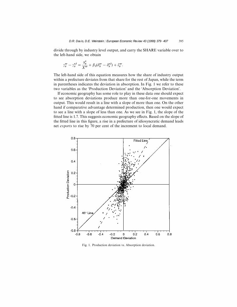
divide through by industry level output, and carry the SHARE variable over tothe left-hand side, we obtain

!!"#

!!!$#

" "!#

X!"##

!($!"

#!$!$

#)#%J !"

#.

The left-hand side of this equation measures how the share of industry outputwithin a prefecture deviates from that share for the rest of Japan, while the termin parentheses indicates the deviation in absorption. In Fig. 1 we refer to thesetwo variables as the ‘Production Deviation’ and the ‘Absorption Deviation’.

If economic geography has some role to play in these data one should expectto see absorption deviations produce more than one-for-one movements inoutput. This would result in a line with a slope of more than one. On the otherhand if comparative advantage determined production, then one would expectto see a line with a slope of less than one. As we see in Fig. 1, the slope of thefitted line is 1.7. This suggests economic geography e!ects. Based on the slope ofthe fitted line in this figure, a rise in a prefecture of idiosyncratic demand leadsnet exports to rise by 70 per cent of the increment to local demand.

Fig. 1. Production deviation vs. Absorption deviation.


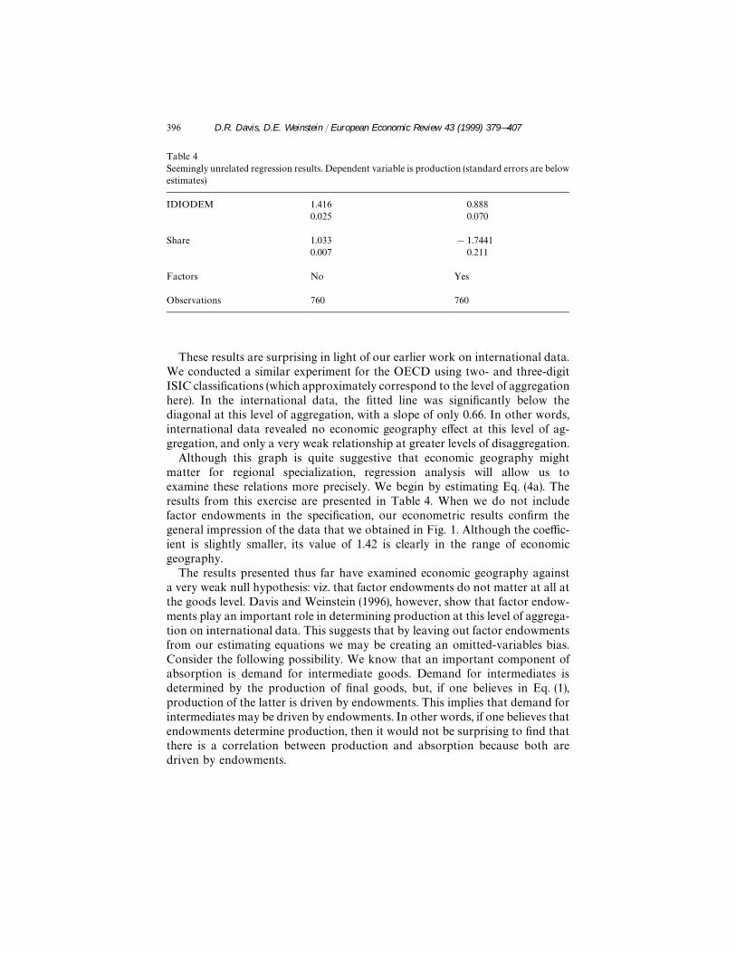
Table 4Seemingly unrelated regression results. Dependent variable is production (standard errors are belowestimates)

IDIODEM 1.416 0.8880.025 0.070

Share 1.033 !1.74410.007 0.211

Factors No Yes

Observations 760 760

These results are surprising in light of our earlier work on international data.We conducted a similar experiment for the OECD using two- and three-digitISIC classifications (which approximately correspond to the level of aggregationhere). In the international data, the fitted line was significantly below thediagonal at this level of aggregation, with a slope of only 0.66. In other words,international data revealed no economic geography e!ect at this level of ag-gregation, and only a very weak relationship at greater levels of disaggregation.

Although this graph is quite suggestive that economic geography mightmatter for regional specialization, regression analysis will allow us toexamine these relations more precisely. We begin by estimating Eq. (4a). Theresults from this exercise are presented in Table 4. When we do not includefactor endowments in the specification, our econometric results confirm thegeneral impression of the data that we obtained in Fig. 1. Although the coe"c-ient is slightly smaller, its value of 1.42 is clearly in the range of economicgeography.

The results presented thus far have examined economic geography againsta very weak null hypothesis: viz. that factor endowments do not matter at all atthe goods level. Davis and Weinstein (1996), however, show that factor endow-ments play an important role in determining production at this level of aggrega-tion on international data. This suggests that by leaving out factor endowmentsfrom our estimating equations we may be creating an omitted-variables bias.Consider the following possibility. We know that an important component ofabsorption is demand for intermediate goods. Demand for intermediates isdetermined by the production of final goods, but, if one believes in Eq. (1),production of the latter is driven by endowments. This implies that demand forintermediates may be driven by endowments. In other words, if one believes thatendowments determine production, then it would not be surprising to find thatthere is a correlation between production and absorption because both aredriven by endowments.


The obvious solution is to estimate Eq. (4b) since it includes factor endow-ments on the right-hand side. The results of this exercise are presented in thesecond column of Table 4. Interestingly, this causes the coe!cient onIDIODEM to decline to 0.9.! This implies that once we account for factorendowments, it no longer is the case that movements in demand produce morethan proportionate movements in production. In other words, this specificationrejects economic geography.

This result is troubling, especially in light of our earlier work. On interna-tional data, we also rejected the economic geography specification, but when wedid so in the specification with factor endowments, we obtained a coe!cient onIDIODEM of 0.3. This implies that in international data, on average less thanone-third of any deviation in demand was met by higher domestic production,the rest being met by imports. This result makes sense in light of the existence ofinternational transaction costs which theoretically can cause demand and pro-duction to covary. What is more puzzling is that if one believes that comparativeadvantage drives production then one should also believe that in regional data,where transportation costs are presumably lower, one should obtain an evensmaller coe!cient on IDIODEM. Instead we have a coe!cient that is too largeto plausibly be generated by comparative advantage and transport costs, buttoo small to signal economic geography.

One explanation for these results is that not all sectors are composed ofmonopolistically-competitive industries. Suppose that only a few of our aggreg-ates actually contain sectors exhibiting increasing returns. Then our system ofequations would be pooling together industries in which the coe!cient onIDIODEM is greater than unity with sectors in which the coe!cient is less thanunity. This pooling could be the explanation for a coe!cient that is too high toplausibly describe a comparative advantage world, but too low to lead us tobelieve that economic geography matters.

Fortunately, it is straightforward to modify our theory to address this prob-lem. Assume that some of our aggregates are composed entirely of constantreturns to scale sectors and others of increasing returns to scale sectors. Then thecorrect test would be to run Eq. (4b) separately for each aggregate. This shouldresult in aggregates without monopolistically-competitive sectors exhibiting lowcoe!cients on IDIODEM, but sectors with increasing returns producing coe!-cients over unity. The results from this exercise are presented in Table 5. In thethree least skill-intensive aggregates, we detect no significant economic geogra-phy e"ect. However, in the more skill-intensive aggregates 4 and 5 we find

!The coe!cient on SHARE typically was negative in specifications with endowments. This islargely due to the high degree of multicollinearity between this variable and the endowments. SinceSHARE simply picks up industry size e"ects that can easily be captured by endowments, weexperimented with omitting the variable and constraining it to equal one. These experiments did notqualitatively alter our results.


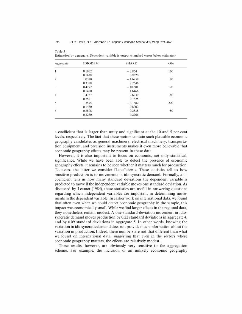
Table 5Estimation by aggregate. Dependent variable is output (standard errors below estimates)

Aggregate IDIODEM SHARE Obs

1 0.1052 !2.864 1600.1628 0.9320

2 1.0320 !1.6958 800.3328 2.2646

3 0.4272 !10.681 1200.1480 1.6466

4 1.4757 2.6239 800.2521 0.7825

5 1.3575 !3.1882 2000.1430 0.8202

6 0.8808 !0.2538 800.2230 0.2766

a coe!cient that is larger than unity and significant at the 10 and 5 per centlevels, respectively. The fact that these sectors contain such plausible economicgeography candidates as general machinery, electrical machinery, transporta-tion equipment, and precision instruments makes it even more believable thateconomic geography e"ects may be present in these data.

However, it is also important to focus on economic, not only statistical,significance. While we have been able to detect the presence of economicgeography e"ects, it remains to be seen whether it matters much for production.To assess the latter we consider !-coe!cients. These statistics tell us howsensitive production is to movements in idiosyncratic demand. Formally, a !-coe!cient tells us how many standard deviations the dependent variable ispredicted to move if the independent variable moves one standard deviation. Asdiscussed by Leamer (1984), these statistics are useful in answering questionsregarding which independent variables are important in determining move-ments in the dependent variable. In earlier work on international data, we foundthat often even when we could detect economic geography in the sample, thisimpact was economically small. While we find larger e"ects in the regional data,they nonetheless remain modest. A one-standard-deviation movement in idio-syncratic demand moves production by 0.22 standard deviations in aggregate 4,and by 0.09 standard deviations in aggregate 5. In other words, knowing thevariation in idiosyncratic demand does not provide much information about thevariation in production. Indeed, these numbers are not that di"erent than whatwe found on international data, suggesting that even in the sectors whereeconomic geography matters, the e"ects are relatively modest.

These results, however, are obviously very sensitive to the aggregationscheme. For example, the inclusion of an unlikely economic geography


candidate, leather, in aggregate 5 may dilute the overall impact of economicgeography in these data. In fact, while we found that changing the basis of ouraggregation scheme had little impact on estimates obtained in the full system,changing the mix of goods within our industry definitions could cause di!erentgroups of industries to be labeled as sectors with significant economic geogra-phy e!ects.

One solution to this theoretical and empirical mire is to foreswearaggregation altogether, and allow all coe"cients to vary at the goods level.This might be appropriate if, contrary to our initial theoretical specification, theelasticity of substitution between varieties of a good is di!erent for thevarious goods within an industry. The results from this exercise are presented inTable 6. The coe"cient on IDIODEM is significantly larger than unity foreight of the 19 sectors: textiles, paper and pulp, iron and steel, chemicals,transportation equipment, precision instruments, non-ferrous metals, andelectrical machinery. With perhaps the exception of paper and pulp, all ofthese seem like plausible candidates for monopolistic competition, with textiles,transportation equipment, iron and steel, and electrical machinery pro-viding canonical examples of the power of the economic geography frame-work (see Krugman, 1991). Furthermore, our results are robust to whicheveraggregation scheme we choose. The variables SHARE and IDIODEMwill vary depending on whether we group industries on the basis of collegeto non-college, capital to non-college ratios, or capital to college ratios.However, we found that all of these sectors except paper and pulp wereidentified as exhibiting economic geography e!ects regardless of the aggregationscheme.

We can run an additional robustness check to confirm that we are identifyingeconomic geography e!ects here. We posit that the R&D-intensity of an indus-try may be used as a proxy for the increasing returns and monopolisticcompetition that underlie the economic geography theory. Fig. 2 plots ourestimated coe"cients against sectoral R&D expenses divided by sales. Thecorrelation is 0.62, indicating that high R&D is associated with identificationof economic geography sectors. In fact, the four most R&D-intensive sectorsare also the four sectors for which we obtain the highest coe"cients onIDIODEM.

Once again we confront the issue of economic significance. We repeat ourexperiment with beta-coe"cients, only this time we use the disaggregated resultspresented in Table 6. Table 7 reports the !-coe"cients for the eight sectors forwhich we obtained statistically significant economic geography coe"cients. Forthese sectors, economic geography seems quite important. A one standarddeviation movement in idiosyncratic demand on average moves production byhalf a standard deviation. In other words, observed fluctuations in idiosyncraticdemand seem to provide a lot of information about production patterns.Furthermore, in the important sector of transportation equipment, these e!ects


Table 6Disaggregated estimation. Dependent variable is output (standard errors below estimates)

Industry Economicgeography

IDIODEM SHARE Factors Adjusted R! Observations

Textile ** 3.9532 0.5932 Yes 0.8468 400.4570 3.2302

Apparel !1.5866 !24.3909 Yes 0.5725 400.2843 4.3741

Lumber 1.0622 4.1937 Yes 0.8106 400.4440 1.8351

Furniture !0.5538 !5.1598 Yes 0.988 400.2765 1.4389

Pulp, paper ** 1.9913 !8.9731 Yes 0.8917 400.3150 1.7861

Printing 0.7269 !0.3423 Yes 0.9979 400.2296 0.2876

Chemicals ** 6.6781 0.9248 Yes 0.9928 401.2454 1.1038

Petrol, !0.4655 !6.3220 Yes 0.9934 40coal products 2.3048 4.2047

Rubber !0.1081 !24.5223 Yes 0.8454 400.1763 5.78042

Leather, 0.1643 !7.1330 Yes 0.9412 40leather products 0.4053 1.7866

Stone, clay, !0.6454 !5.0674 Yes 0.7681 40glass 0.4148 2.4824

Iron, steel ** 3.9294 !3.9582 Yes 0.7663 400.5613 6.2968

Non-ferrous ** 1.5932 2.5509 Yes 0.962 40metals 0.1741 3.1334

Fabricated !0.8197 !14.0257 Yes 0.5972 40metal 1.0820 7.0734

General !0.4219 !4.4744 Yes 0.7802 40machinery 0.9524 2.6163

Electrical ** 6.2713 5.6614 Yes 0.9002 40machinery 1.3552 3.7628

Transport ** 6.7060 1.2685 Yes 0.8826 40equipment 0.5024 0.9336

Precision ** 4.32139 !3.9460 Yes 0.7477 40instruments 0.8115 1.8107

Other 0.0655 1.1179 Yes 0.5307 40manufacturing 0.3824 1.4888

Note: Asterisks indicate that the coe!cients on IDIODEM are significantly large than one at the 5%level.

are very strong. Although economic geography may not be that important forinternational specialization, there appears to be strong evidence that it mattersfor certain sectors on a regional level.


Fig. 2. Coe!cient on IDIODEM vs. R&D Intensity.

Table 7Beta coe!cients for goods with significant coe!cients on IDIODEM

Sector Beta coe!cient

Textiles 0.82Iron and steel 0.40Paper and pulp 0.51Transportation equipment 0.74Non-ferrous metals 0.42Electrical machinery 0.37Precision instruments 0.42Chemicals 0.53

4. Conclusion

This paper investigates the existence and importance of economic geographye"ects in determining production structure for a sample of regions of Japan.


Results from this regional work both complement and contrast with those ofDavis and Weinstein (1996) based on a sample of OECD countries. Within thehypothesis testing framework developed, the earlier work found scant supportfor the economic geography framework in the international sample. Moreover,even insofar as it was possible to statistically identify such e!ects, their economicsignificance was very minimal.

The regional data prove much more supportive of the economic geographyhypothesis. We find statistically significant e!ects of economic geography foreight of nineteen manufacturing sectors: transportation equipment, iron andsteel, electrical machinery, chemicals, precision instruments, nonferrous metals,textiles, and paper and pulp. Moreover, for many of these sectors, the economicgeography e!ects are likewise very significant in economic terms.

Why are the regional e!ects of economic geography so strong, while theinternational e!ects are so weak? We suspect two principal reasons. The first istrade costs: both transport costs and myriad barriers to trade must surely belower for trade between regions of a country than between countries. In theeconomic geography framework, lower (but strictly positive) trade costs lead tostronger e!ects, as this reflects lower implicit protection for production in therelatively smaller markets. The second likely reason is the greater mobilityof factors across regions than countries. The suggestion is that such mobilitywill tend to reinforce the economic geography e!ects, relieving scarcities inregions favorable on economic geography grounds for production of particulargoods.

How do these new results a!ect the conclusions of our earlier work regardingthe significance of economic geography in determining production specializa-tion within the OECD? They bring our earlier work into sharper focus in tworespects. First, our earlier work had found weak evidence of economic geogra-phy e!ects in as many as one-third of the goods that comprise our sample. Sincethe microeconomic story that one tells at the regional and international level isby and large the same, this strengthens our confidence that we had in factidentified economic geography e!ects in the international data. The fact that wefind the economic significance of economic geography to be greater in theregional data is exactly what one would expect. This likewise gives us greaterconfidence that our methodology is not inherently biased against finding impor-tant economic geography e!ects. Hence, it tends to strengthen our confidence inour earlier finding that economic geography does not matter a great deal inunderstanding the structure of international production.

The sharp contrast in the economic significance of economic geography e!ectsacross regions versus internationally is a strong caution against accepting theview that the boundary between international and interregional economics is onthe verge of vanishing due to reductions in border barriers. As such, thisreinforces the perspective o!ered in McCallum (1995) and Engel and Rogers(1996) that national borders continue to matter a great deal. Moreover, the


strength of the economic geography e!ects on the regional data suggest thatif the future holds a time when international trade costs truly do fall to the levelof interregional trade costs, then quite substantial international restructuring ofindustry may be in the o"ng.

The empirical approach to identifying economic geography e!ects that weemploy in this paper is novel. In order to keep our framework simple, we haveset to the side a large number of important analytic and empirical questions.These include the roles of absolute market size, forward- and backward-link-ages, and ‘real-world’ geography. Naturally, the results reported here should beinterpreted with an understanding that many issues in this area remain to beexplored.

In sum, economic geography appears to be very important in determining thestructure of production across regions of Japan for eight of nineteen manufac-turing sector. In contrast to Davis and Weinstein (1996), which in exactly thesame framework had shown scant economic significance of economic geographyfor the structure of OECD production, here we find that it is very important forthe structure of regional production.

Acknowledgements

The first author is grateful to the Harvard Institute for International Develop-ment for funding for this project. Trevor Reeve once again provided first-rateresearch assistance. The views expressed in this paper are those of the authors,and not those of supporting institutions, the Federal Reserve Bank of New Yorkor the Federal Reserve System.

Appendix A: Data

Prefectural endowments

The numbers of workers by educational attainment were entered byprefecture directly from the Employment Status Survey of 1987 (ShugyoKozo Kihon Chosa Hokoku). The capital stocks were imputed from prefecturalinvestment data. Japan’s yearly Annual Report on Prefectural Accounts (KenminKeizai Keisan Nempo) give investment flows for each prefecture from 1975to 1985. These flows were used to impute capital stock levels for each pre-fecture in 1985, using capital goods price deflators from the Annual Report onNational Accounts (Kokumin Keizai Keisan Nempo) and a rate of depreciation of0.133 (This was the same rate of depreciation used by Bowen et al. (1987)). Eachyear’s flow was deflated using a capital deflator from the NationalAccounts.


Prefectural production

Shipment data for 20 manufacturing sectors in each prefecture were takenfrom the Japanese Census of Manufactures for 1985. The gross output of 9 non-manufacturing sectors in each prefecture was taken from the Prefectural Ac-counts for 1985. Finally, these totals were scaled so that the 47-prefectural totalfor each sector exactly matched the total Japanese output as reported in the1985 Input—Output !able of Japan. Thus, in e!ect, the data from the Census ofManufactures and from the Prefectural Accounts was used in order to distributetotal Japanese output for each sector across the 47 prefectures as accurately aspossible.

!echnology

Each element of the 3!29 technology matrix B was calculated by dividingJapanese total output for the 29 sectors into the number of each factor present ineach sector. Most of the data on college and non-college workers in each sectorcame from the 1988 "age Census (Chingin Sensasu). There were some gaps inthis data as follows: (1) There was no data for college and non-college workersfor agriculture, forestry, and fisheries or for government. These numbers weretaken from the 1987 Employment Status Survey (Showa 63 Nen Shugyo KozoKihon Chosa Hokoku Chiiki Hen I II). (2) There was also no data for thepetroleum/coal and leather industries. Total employment for each of thesesectors was taken from the 1985 Census of Manufactures. The number of collegeworkers per unit output for each was then imputed by assuming that petro-leum/coal has the same fraction of college workers as the chemicals sector andthat leather has the same fraction as manufacturing overall. The capital stocks ineach of the 30 sectors were imputed from investment numbers, using the AnnualReport of the Corporation Survey for non-manufacturing and the Census ofManufactures for manufacturing.

Absorption

Intermediate input use in each region was calculated using the Japan 30!30IO matrix for 1985. Thus, INPUT r"AX r, where INPUT r is intermediateconsumption in region r, A is the IO matrix, and X r is gross output in region r.Both INPUT r and X r, therefore, are 30!1 vectors. The 47 INPUT r vectorstogether form a 30!10 intermediate consumption matrix. It is important tonote that one of our sectors in both A and X r is producers of governmentservices. Government absorption is therefore included in INPUT r.

The construction of the consumption data was quite complex. In 1984, theJapanese government performed a detailed survey of Japanese consumption onthe prefectural level, the National Survey of Income and Expenditure, that brokeJapanese household consumption up into 65 categories. Unfortunately this data


cannot be easily concorded into the 30 industrial categories that we use in thepaper. However the Economic Planning Agency does provide a 30!42 bridgingmatrix which map the 42 consumption commodities that can easily be formedfrom the 56 consumption categories in the Family Income and ExpenditureSurvey for 1987 into 30 core sectors corresponding to the Japanese IO table.Unfortunately this second source of data only reports information for tenJapanese regions. Since the 65 categories of the National Survey of Income andExpenditure did not always correspond to the 56 categories of the FamilyIncome and Expenditure Survey, we used the following procedure to developconsistent series. First, for most categories there was a perfect match betweenthe two sources, so we used the National Survey of Income and Expenditure forentries wherever possible. We then used regional totals scaled by householdincome shares to fill in the gaps. Since we were using both 1984 and 1987 data allprefectural entries were scaled so that they matched the regional totals.

These data were then aggregated up to 42 categories, producing a 42!47matrix of final consumption by region. The survey data was based, of course,on consumer prices, so the bridge matrix was specially constructed to translatethe consumption expenditure into producer prices. Most of the di!erencebetween consumer and producer prices results from wholesale and retailmarkups and from transportation costs, so the mapping shifted portions ofspending on each final good into the wholesale/retail trade and transportationsectors, reflecting the fact that to consume anything bought retail is to consumethe wholesaling, retailing, and transportation services which brought the prod-uct to the store. Without this adjustment, the data would have greatly under-estimated final consumption of wholesale/retail and transportation services andwould have shown each region exporting far more of these services than isplausible.

There are no investment figures broken down for 30 sectors and 47 prefectures,so these numbers were imputed using IO Table investment data. The IO Tablebreaks down investment into the 30 sectors for Japan as a whole. This vector wasthen distributed across regions, using as weights each region’s share in totalinvestment for Japan as a whole. Thus, INV r"(!I!/!I")INV J, where INV r isa 30!1 investment vector for region r, !I ! is the total investment for that regionin 1985 (taken from the prefectural accounts), !I " is Japan’s total investment for1985, and INV r is the 30!1 investment vector taken from the IO Table. These 10INV’s therefore formed a 30!10 investment matrix. Business consumption wasadded to the data in a similar fashion. The data for all prefectures was thenaggregated into 29 sectors to make it compatible with our B matrix.

R&D Data

Research and Development data was taken from the Report on the Survey ofResearch and Development.


References

Bernstein, J., Weinstein, D., 1997. Do endowments predict the location of production? Evidencefrom national and international data. Mimeo., University of Michigan, East Lansin.

Bowen, H.P., Leamer, E., Sveikauskas L., 1987. Multicountry, multifactor tests of the factorabundance theory. American Economic Review 77.

Chipman, J.S., 1992. Intra-industry trade, factor proportions and aggregation. Economic Theoryand International Trade: Essays in Memoriam of J. Trout Rader. Springer, New York.

Davis, D.R., 1995. Intra-industry trade: A Heckscher—Ohlin—Ricardo approach. Journal of Inter-national Economics 39.

Davis, D.R., 1997. Critical evidence on comparative advantage? North—North trade in a multilateralworld. Journal of Political Economy 97, Oct.

Davis, D.R., Weinstein, D.E., 1996. Does economic geography matter for international specializa-tion. Working paper no. 5706, NBER, Cambridge, MA.

Davis, D.R., Weinstein, D.E., Bradford, S.C., Shimpo, K., 1997. Using international and Japaneseregional data to determine when the factor abundance theory of trade works. AmericanEconomic Review 87, June.

Deardor!, A.V., 1998. Determinants of bilateral trade: does gravity work in a neoclassical world? In:Je!rey, F. (Ed.), Regionalization of the World Economy. U. of Chicago and NBER, Chicago.

Dixit, A.K., Stiglitz, J.E., 1977. Monopolistic competition and optimum product diversity. AmericanEconomic Review 67 (3), 297—308.

Ellison, G., Glaeser, E.L., 1997. Geographic concentration in U.S. manufacturing industries: A dart-board approach. Journal of Political Economy 105 (5), 889—927.

Engel, C., Rogers, J.H., 1996. How wide is the border? American Economic Review 86.Glaeser, E.L. et al., 1992. Growth in cities. Journal of Political Economy 100 (6), 1126—1152.Helpman, E., 1981. International trade in the presence of product di!erentiation, economies of scale

and monopolistic competition: A Chamberlin—Heckscher—Ohlin approach. Journal of Interna-tional Economics 11 (3).

Henderson, J.V., 1986. E"ciency of resources usage and city size. Journal of Urban Economics 19(1), 47—70.

Henderson, J.V., Kuncoro, A., Turner, M., 1995. Industrial development in cities. Journal of PoliticalEconomy 103 (5), 1067—1090.

Justman, M., 1994. The e!ect of local demand on industry location. Review of Economics andStatistics 76 (4), 742—753.

Krugman, P., 1979. Increasing returns, monopolistic competition, and trade. Journal of Interna-tional Economics 9 (4).

Krugman, P.R., 1980. Scale economies, product di!erentiation, and the pattern of trade. AmericanEconomic Review 70, 950—959.

Krugman, P.R., 1991. Geography and Trade. MIT Press, Cambridge, MA.Krugman, P.R., 1994. Empirical evidence on the new trade theories: The current state of play. In:

New Trade Theories: A Look at the Empirical Evidence. Center for Economic Policy Research,London.

Krugman, Venables, 1995. Globalization and the inequality of nations. Quarterly Journal ofEconomics CX (4).

Leamer, E., 1984. Sources of International Comparative Advantage: Theory and Evidence. MITPress, Cambridge, MA.

Linder, S.B., 1961. An Essay on Trade and Transformation. Wiley, New York.McCallum, J., 1995. National borders matter: Canada—US regional trade patterns. American

Economic Review 85 (3).Nakamura, R., 1985. Agglomeration economies in urban manufacturing industries: A case of

Japanese cities. Journal of Urban Economics 17 (1), 108—124.


Sveikauskas, L.A., 1975. The productivity of cities. Quarterly Journal of Economics 89 (3), 393—413.Sveikauskas, L.A., Gowdy, J., Funke, M., 1988. Urban productivity: City size or Industry size?

Journal of Regional Science 28 (2) 185—202.Weder, R., 1995. Linking absolute and comparative advantage to intra-industry trade theory.

Review of International Economics 3 (3).


Documents

Economic geography and regional production structure: An ...blogs.cuit.columbia.edu/dew35/files/2016/08/Economic_Geography... · economic geography featuring ‘home market eﬀects’