Production, 26(4), 698-706, out./dez. 2016

http://dx.doi.org/10.1590/0103-6513.209916

1. Introduction

Control charts are commonly used as a statistical tool for online process control, to maintain the measurement of quality characteristics of the product produced in between certain limits known as upper control limit (UCL) and lower control limit (LCL). The target value of the process location is set and is referred to as centre line (CL). This tool is first developed by Shewhart (1931). Since then, it is used worldwide for the control of statistical as well as economic performance of the process. In statistical control charts, the overall concentration is made to maintain the statistical constants of the chart such as type I error probability (α), power (1-β) of the chart etc. whereas, in the economic design of control chart, process is targeted to minimize overall loss from the process so that, process can earn maximum profit. In the literature, there are so many types of control charts such as, mean and range (X and R) charts, moving average charts, exponentially weighted moving

average (EWMA) charts, cumulative sum (CUSUM) charts etc. There are some charts designed also for attribute data which are, control chart for number of defectives (d chart), control charts for number of defects (c chart), control charts for fraction defectives (np chart) etc. Also, there are some non-parametric charts such as sign chart, signed rank chart etc. All these charts have their own statistical properties.

In the economic design of control charts, an expression for the loss (gain) per unit time or per unit produced is obtained, and is optimized with respect to the design parameters; sample size (n), sampling interval (h) and control limit multiplier (k) in terms of sigma units. Duncan (1956) first introduced an economic design for X control chart by applying numerical method to obtain optimal values of design parameters that optimizes the loss cost from the process design. Since then, considerable work on economic design of control charts is carried

Received: Mar. 29, 2016; Accepted: Aug. 30, 2016

Economic design of a nonparametric EWMA control chart for location

Patil Subhash Haribaa*, Shirke Digambar Tukaramb

aDoodhsakhar Mahavidyalaya, Bidri, Dist-Kolhapur, State-Maharashtra, IndiabShivaji University, Kolhapur, Dist-Kolhapur, State-Maharashtra, India

*psubhash_2007@rediffmail.com

Abstract

In this article, we have proposed an economic design of Exponentially Weighted Moving Average control chart based on sign statistic to control location parameter of the process. The economic performance of the chart is evaluated for different shifts in the location. It is observed that, as shift in the process location increases, sample size to detect the shift and the loss cost from the process decrease. The power of the chart increases with increasing shift. The design gives better economic/statistical performance for large shifts in the process. This economic procedure can be applied to any process having known or unknown process outcome distribution. The sensitivity of the design is also carried out to check the effect on statistical as well as economic performance of the design due to change in different time and cost parameters.KeywordsEconomic design. Production cycle. EWMA control chart. Markov chain. Expected loss.

How to cite this article: Patil, S. H., & Shirke, D. T. (2016). Economic design of a nonparametric EWMA control chart for location. Production, , 26(4), 698-706, out./dez. 2016http://dx.doi.org/10.1590/0103-6513.209916.

Economic design of a nonparametric ... control chart for location. Production, 26(4), 698-706, out./dez. 2016699

Patil, S. H. et al.

out; Montgomery (1980) has reported a review of it up to 1980. Rahim (1985, 1989) has obtained an economic design of X chart under non-normality and obtained optimal design parameters for X and R chart. Lorenzen & Vance (1986) proposed unified approach for economic design of control charts. Saniga (1989) has obtained economic-statistical design of X and R chart, which gives economic design with improved statistical properties at slight increase in loss cost. The considerable work on economic design of control charts is also carried out by Banerjee & Rahim (1987), Reynolds Junior et al. (1988), McWillims (1989), Koo & Case (1990), Bai & Lee (1998), Chou et al. (2001), Chen (2004), Chen & Yeh (2006), Mahadik & Shirke (2007), Patil & Rattihalli (2009), Yeh & Chen (2010), Patil & Shirke (2015) and many others. The work by these researchers has made consistent improvement in the economic design of different types of control chart.

It is observed that, though the CUSUM and/or EWMA charts are effective to detect the small and moderate shifts in the process, less is reported on economic design of these control charts. Further, the practitioners, as they are not aware of these charts, also avoid using these charts. In review of the work on economic design of CUSUM/EWMA chart, we observe; Pan & Chen (2005) have obtained economic design of CUSUM chart for monitoring environmental performance, Serel & Moskowitz (2008) have obtained an economic design of EWMA control chart to monitor process mean and variance jointly using quadratic loss function. Serel (2009) has developed economic EWMA control chart using linear, quadratic and exponential loss function. He et al. (2009) has obtained economic design of EWMA control chart based on Average Run Length (ARL) using response surface methodology (RSM) to search the optimal set of EWMA parameters. Saghaei et al. (2014) have developed economic design of EWMA control chart based on measurement errors using Genetic Algorithm (GA). Chiu (2015) has obtained economic-statistical design of EWMA chart based on quadric loss function using Lorenzen & Vance (1986) approach. Chiu (2015) has used nonlinear programming with statistical constraints to obtain optimum loss per unit time.

Observing this literature, in the present study, an attempt is made to obtain an economic design of EWMA control chart proposed by Yang et al. (2011a) to monitor shifts in the process location. A nonparametric EWMA sign statistic based on signs of observations from the process target value is considered. The nonparametric sign static is used as is independent of process distribution and hence can easily be applied to any control procedure. Only we

need to calculate signs of observations from target location. Another advantage is the knowledge of process variance is not required for the implementation of the sign control chart. To reach the purpose, an expression for expected loss cost per unit time is obtained and is minimized with respect to the design parameters of EWMA control chart. An expression for loss cost per unit time is obtained by taking a ratio of the expressions for expected loss cost during a production cycle and expected length of the cycle [Montgomery (1980, 2008)]. The study is aimed to use EWMA chart effectively in economic point of view so that, professionals can use it for any type of process distribution (normal or non-normal). The paper consists of six sections. Section 2, followed by this section describes construction of the EWMA control chart based on sign statistic. The process design is given in section 3. Expressions for expected cycle length and expected loss cost during the production cycle are given in section 4. An example and the sensitivity of the design are carried out in section 5. Conclusions are given in section 6 followed by the references.

2. The EWMA control chart based on sign statistic

Suppose ‘X’ is a process characteristic of a production process and have a continuous distribution with cumulative distribution function F(.). The process is targeted to control a process location µ having target value µ0.

Let xij, i=1, 2, ….; j=1, 2, … n. be a jth observation from a sub-group sample of size n observed at ith sampling epoch from this process with target location µ=µ0.

Define,

ij 0

j

1 ; x

Y0 ;

if

otherwise

> µ

= (1)

then, Si = ΣYj, represents one sided sign statistic and gives number of x values in a sample of size n exceeding process target value µ=µ0 at ith sampling epoch. Now, Si becomes a discrete random variable and has binomial distribution with parameters (n, p), where p=P(xij> µ0). If the process location is at median of the process, we have p=1/2 and E(Si)=n/2. If the process location is different from median, value of p will be different than 1/2.

This sign statistic is a slight modification of two sided sign statistic used by Amin et al. (1995) to construct a nonparametric sign control chart. Khilare & Shirke (2010) has also used the sign statistic to

Economic design of a nonparametric ... control chart for location. Production, 26(4), 698-706, out./dez. 2016700

Patil, S. H. et al.

develop nonparametric synthetic control chart. The EWMA statistic to monitor small shifts in the process location based on sign statistic is defined as,

( ) 1 1iS i iEWMA S Sλ λ −= + − (2)

where, 0 < λ ≤ 1, is a smoothing parameter of EWMA control chart. The starting value of EWMA, denoted as

0SEWMA is taken to be the mean value of S, given by np and have value n/2, if the process location is at median of the process.

The control limits for EWMA chart for long run time according to Yang et al. (2011a) are given by,

( )

( )

1 ,2

,

1 ,2

UCL np k np p

CL np

LCL np k np p

λλ

λλ

= + −−

=

= − −−

(3)

where, k and λ are the properly chosen parameters of EWMA chart, so as to attain certain average run length (ARL), when process is in control.

The ARL of the control chart can be calculated based on Markov Chain approach by Brook & Evans (1972) or by approach by Lucas & Saccucci (1990). To obtain ARL of the chart, the in-control region (LCL, UCL) of the control chart is divided into (N-1) sub-intervals of equal width, representing transient states and Nth state is an absorbing state. P={pij} be the (N-1)×(N-1) transient probability matrix representing probabilities of moving to state j from state i in one step. These probabilities are calculated using approach by Lucas & Saccucci (1990) and are given by,

pij= P(moving to state Sj/ being in state Si previously)

=P(EWMA ∈ Sj at time t /EWMA ∈ Si at time (t-1)).

If, b= (b1, b2, …, bN-1)' is a column matrix of order (N-1) of initial probabilities and 1= (1, 1, …, 1)' is a

column matrix of order (N-1) having each element equal to one, then the ARL of the control chart is given by,

ARL = b'(1-P)1 (4)

This formula of ARL can be used to find in-control and out-of-control ARL’s of this EWMA control chart. If we use p, as in-control probability (say p0), the ARL computed is in-control ARL usually denoted by ARL0 and when we use p as out-of-control probability (say p1), the ARL computed be out-of-control ARL usually denoted by ARL1. For an illustration, consider EWMA scheme monitored by EWMA chart with parameters λ=0.2 and k=2.84. The in-control and out-of-control ARL values for this chart are as given in Table 1 and Table 2 respectively for different p values. Out-of-control ARL’s obtained in Table 2 are for the shift in median.

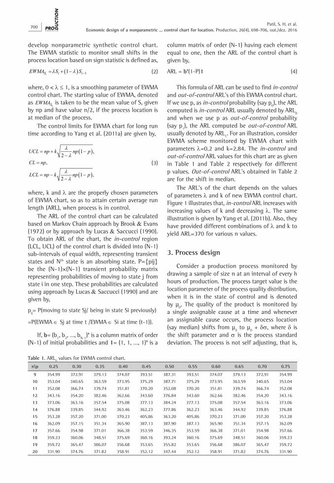
The ARL’s of the chart depends on the values of parameters λ and k of new EWMA control chart. Figure 1 illustrates that, in-control ARL increases with increasing values of k and decreasing λ. The same illustration is given by Yang et al. (2011b). Also, they have provided different combinations of λ and k to yield ARL=370 for various n values.

3. Process design

Consider a production process monitored by drawing a sample of size n at an interval of every h hours of production. The process target value is the location parameter of the process quality distribution, when it is in the state of control and is denoted by µ0. The quality of the product is monitored by a single assignable cause at a time and whenever an assignable cause occurs, the process location (say median) shifts from µ0 to µ0 + δσ, where δ is the shift parameter and σ is the process standard deviation. The process is not self adjusting, that is,

Table 1. ARL0 values for EWMA control chart.

n\p 0.25 0.30 0.35 0.40 0.45 0.50 0.55 0.60 0.65 0.70 0.75

9 354.99 372.91 379.13 374.07 393.51 387.31 393.51 374.07 379.13 372.91 354.99

10 353.04 340.65 363.59 373.95 375.29 387.71 375.29 373.95 363.59 340.65 353.04

11 352.08 366.74 339.74 351.81 370.20 352.08 370.20 351.81 339.74 366.74 352.08

12 343.16 354.20 382.46 362.66 343.60 376.84 343.60 362.66 382.46 354.20 343.16

13 373.06 363.16 357.54 375.08 377.13 384.24 377.13 375.08 357.54 363.16 373.06

14 376.88 339.85 344.92 363.46 362.23 377.86 362.23 363.46 344.92 339.85 376.88

15 353.28 357.20 371.00 370.23 405.86 363.20 405.86 370.23 371.00 357.20 353.28

16 362.09 357.15 351.34 365.90 387.13 387.90 387.13 365.90 351.34 357.15 362.09

17 357.66 354.98 371.01 366.38 353.59 346.35 353.59 366.38 371.01 354.98 357.66

18 359.23 360.06 348.51 375.69 360.16 393.24 360.16 375.69 348.51 360.06 359.23

19 359.72 365.47 386.07 356.68 353.65 355.82 353.65 356.68 386.07 365.47 359.72

20 331.90 374.76 371.82 358.91 352.12 347.44 352.12 358.91 371.82 374.76 331.90

Economic design of a nonparametric ... control chart for location. Production, 26(4), 698-706, out./dez. 2016701

Patil, S. H. et al.

the process remains in out-of-control state, unless and until human interference.

The process is assumed to be start in the state of control. After some random period shift occurs in the process. Consequently, the process signals and will be brought back in control by removing an assignable cause. This period from starting of the process, till drawing back it in the state of control, when an assignable cause occurs in between them is termed to be one production cycle. That is, the time between two successive in-control states, given that the shift occurs in between them is known to be one production cycle. After this a fresh cycle begins. For figure of production cycle one can refer Patil & Rattihalli (2009). Further, the transaction between in-control and out-of-control states is assumed to be instantaneous. In the economic design of control chart, the time required for completing a production cycle and the expected loss during this cycle is determined, which is used to find an expression for expected loss per unit time during a cycle. This expression for expected loss cost is then minimized with respect to design parameters of the control chart to get an economic design.

The notations used in the economic procedure are as below.

n: sample size.

h: sampling interval length in hours.

k, λ: parameters of EWMA control chart scheme.

θ: parameter of the exponential lifetime distribution for in-control state.

α: probability of false alarm (probability of Type I error).

β: probability of type II error.

s: expected number of samples taken during in-control period.

τ: time of occurrence of the shift in between two consecutive samples.

D: expected search and repair time of an assignable cause during the true alarm.

V0: per hour income from the process when the process is in-control.

V1: per hour income from the process when the process is out-of-control.

C: expected penalty cost per hour due to nonconformities produced while running the process in out-of-control state.

E(T): expected length of the production cycle.

E(A): expected income from the process during the production cycle.

E(I): expected income per hour from the process.

ARL1: out-of-control average run length.

ATS: average time to signal.

N: no. of samples taken during the production cycle.

g: time to sample, inspect and conclude one unit in the sample.

a, b: fixed and variable costs of sampling, respectively.

Table 2. ARL1 values for EWMA control chart.

n\p 0.25 0.30 0.35 0.40 0.45 0.50 0.55 0.60 0.65 0.70 0.75

9 5.20 7.27 11.84 25.71 94.32 387.31 94.32 25.71 11.84 7.27 5.20

10 4.80 6.67 10.77 23.22 86.76 387.71 86.76 23.22 10.77 6.67 4.80

11 4.42 6.08 9.64 20.26 74.75 352.08 74.75 20.26 9.64 6.08 4.42

12 4.27 5.82 9.15 19.15 72.40 376.84 72.40 19.15 9.15 5.82 4.27

13 4.07 5.52 8.60 17.84 68.13 384.24 68.13 17.84 8.60 5.52 4.07

14 3.82 5.16 8.02 16.51 63.32 377.86 63.32 16.51 8.02 5.16 3.82

15 3.63 4.90 7.54 15.31 58.14 363.20 58.14 15.31 7.54 4.90 3.63

16 3.55 4.76 7.29 14.73 56.84 387.90 56.84 14.73 7.29 4.76 3.55

17 3.38 4.49 6.78 13.39 50.17 346.35 50.17 13.39 6.78 4.49 3.38

18 3.27 4.36 6.63 13.22 51.25 393.24 51.25 13.22 6.63 4.36 3.27

19 3.17 4.20 6.30 12.34 46.47 355.82 46.47 12.34 6.30 4.20 3.17

20 3.05 4.03 6.02 11.67 43.58 347.44 43.58 11.67 6.02 4.03 3.05

Figure 1. Effect of λ and k on in-control ARL (ARL0).

Economic design of a nonparametric ... control chart for location. Production, 26(4), 698-706, out./dez. 2016702

Patil, S. H. et al.

V: loss cost for search of an assignable cause due to single false alarm.

W: loss cost for search and repair of an assignable cause during true alarm.

4. Expected cycle length and loss cost

To obtain an expression for expected loss cost per hour, we have to obtain expressions for expected time period required for a production cycle and the expected loss occurred during that cycle. The expected cycle length consists of an in-control period, out-of-control period, time for sampling and testing and the time for search and repair of an assignable cause.

The lifetime of the process is always monitored by a failure time (decay) distributions like Exponential distribution (Poisson process) or Weibull distribution, etc. Let us assume that, an assignable cause occurs according to a Poisson process with rate θ, that is, time to occur an assignable cause has an exponential distribution with mean 1/θ. Hence, the expected in-control time becomes 1/θ.

Therefore,

In-control Time = ICT = 1/θ (5)

Assuming, the shift occurs between ith and (i+1)th sample, the expected time of occurrence of an assignable cause in between ith and (i+1)th sample (τ) according to Montgomery (1980) is,

( ) ( )( )

( )( )

i 1 h tih

i 1 h tih

h

h

t ih e dt,

e dt

e 1 h .

e 1

+ −θ

+ −θ

θ

θ

θ −τ =

θ

− + θ=

θ −

∫∫ (6)

This gives,

ATS = h*ARL1–τ (7)

Therefore, Expected cycle length, which is the time required to complete a cycle is,

E(T) = ICT + ATS + gn + D,

which can be written as,

E(T) = 1/θ + h*ARL1 - τ + gn + D (8)

Equation 8 represents, an expression for expected cycle length of a production cycle.

Now, the expected loss cost occurred during a production cycle consist of the loss due to nonconformities produced during the production cycle, loss occurred due to unwanted search of an assignable cause when

there is a false alarm, cost for sampling and testing and cost for search and repair of an assignable cause when there is true alarm.

The loss occurred due to nonconformities produced is the difference in the income during in-control and out-of-control states of the process. Since, V0 and V1 are the income per hour from the process, when the process is in in-control and out-of-control states respectively, providing C = V0 – V1as the penalty loss cost due to excess number of nonconformities produced while running the process in out-of-control state.

The income from the process during a production cycle is now given by,

( ) [ ]01 1

VE A V h*ARL gn D= + − τ + +θ

(9)

which can be written as,

( ) [ ] [ ]00 1 1

VE A V h*ARL gn D C h*ARL gn D= + − τ + + − − τ + +θ

(10)

This gives expected income per hour as,

( ) ( )( )

E AE I

E T= (11)

[ ]( )

10

C h*ARL gn DV

E T− τ + +

= − (12)

Hence, the loss cost per hour due to non-conformities produced (L1), during a production cycle is given by,

( )[ ]

( )

1 0

11

– ,

C h*ARL gn DL

E T

L V E I=

− τ + +=

(13)

The expected number of samples taken during

the cycle, E(N) are, ( ) ( )E TE N

h= , which gives, the cost

for sampling and testing per hour (L2) as,

2a bnL

h+

= (14)

Now, if s denotes expected number of samples taken during in-control period and P(i), be the probability that shift occurs during ith and (i+1)th sample, then according to Lorenzen & Vance (1986),

( )( )i 1 h

t

ih

e dtP i+

−θ= θ∫ (15)

and,

( )

( )

i

i 1 hih

i 0h

h

s iP i ,

i e e ,

e .1 e

∞−θ +−θ

=−θ

−θ

=

= −

=−

∑

∑ (16)

Economic design of a nonparametric ... control chart for location. Production, 26(4), 698-706, out./dez. 2016703

Patil, S. H. et al.

Since, α is the probability of false alarm, V is the cost for search of an assignable cause when there is false alarm and W is the cost for search and repair of an assignable cause when there is true alarm, then cost per hour for search and repair of an assignable cause (L3) is,

( )3V s WL

E Tα +

= (17)

From Equations 13, 14 and 17, the expected total loss cost per hour during a production cycle is,

( ) 1 2 3E L L L L= + + (18)

Equation 18 represents the equation for the loss cost per unit time from the process during a production cycle. This loss cost function can be minimized with respect to the design parameters of a EWMA control chart, under the condition that, an out-of-control probability (p1) of the process is known. A computer program in MATLAB using pattern search method is written for expected loss cost E(L) in Equation 18 and is optimized for different values of n to get optimum design of the EWMA control chart. This program can be operated for different values of design parameters in possible range so as to reach minimum possible loss from the process design. The illustration using real life example is given in the following section 5.

5. An example

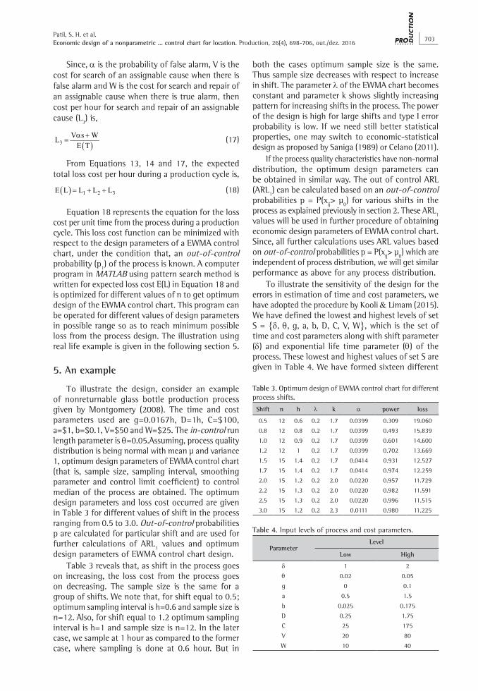
To illustrate the design, consider an example of nonreturnable glass bottle production process given by Montgomery (2008). The time and cost parameters used are g=0.0167h, D=1h, C=$100, a=$1, b=$0.1, V=$50 and W=$25. The in-control run length parameter is θ=0.05.Assuming, process quality distribution is being normal with mean µ and variance 1, optimum design parameters of EWMA control chart (that is, sample size, sampling interval, smoothing parameter and control limit coefficient) to control median of the process are obtained. The optimum design parameters and loss cost occurred are given in Table 3 for different values of shift in the process ranging from 0.5 to 3.0. Out-of-control probabilities p are calculated for particular shift and are used for further calculations of ARL1 values and optimum design parameters of EWMA control chart design.

Table 3 reveals that, as shift in the process goes on increasing, the loss cost from the process goes on decreasing. The sample size is the same for a group of shifts. We note that, for shift equal to 0.5; optimum sampling interval is h=0.6 and sample size is n=12. Also, for shift equal to 1.2 optimum sampling interval is h=1 and sample size is n=12. In the later case, we sample at 1 hour as compared to the former case, where sampling is done at 0.6 hour. But in

both the cases optimum sample size is the same. Thus sample size decreases with respect to increase in shift. The parameter λ of the EWMA chart becomes constant and parameter k shows slightly increasing pattern for increasing shifts in the process. The power of the design is high for large shifts and type I error probability is low. If we need still better statistical properties, one may switch to economic-statistical design as proposed by Saniga (1989) or Celano (2011).

If the process quality characteristics have non-normal distribution, the optimum design parameters can be obtained in similar way. The out of control ARL (ARL1) can be calculated based on an out-of-control probabilities p = P(xij> µ0) for various shifts in the process as explained previously in section 2. These ARL1 values will be used in further procedure of obtaining economic design parameters of EWMA control chart. Since, all further calculations uses ARL values based on out-of-control probabilities p = P(xij> µ0) which are independent of process distribution, we will get similar performance as above for any process distribution.

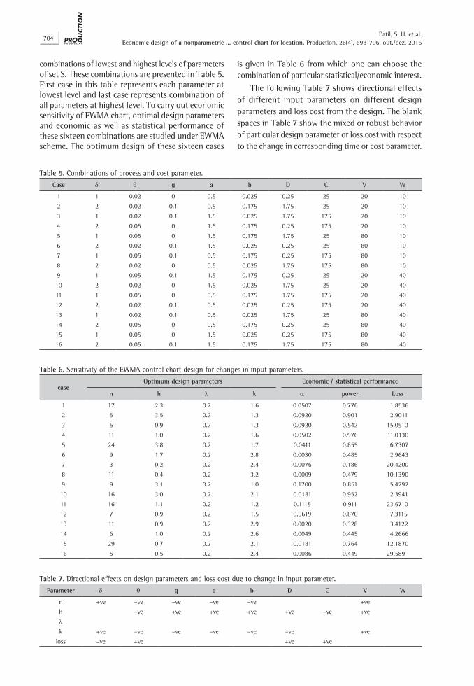
To illustrate the sensitivity of the design for the errors in estimation of time and cost parameters, we have adopted the procedure by Kooli & Limam (2015). We have defined the lowest and highest levels of set S = {δ, θ, g, a, b, D, C, V, W}, which is the set of time and cost parameters along with shift parameter (δ) and exponential life time parameter (θ) of the process. These lowest and highest values of set S are given in Table 4. We have formed sixteen different

Table 3. Optimum design of EWMA control chart for different process shifts.

Shift n h λ k α power loss

0.5 12 0.6 0.2 1.7 0.0399 0.309 19.060

0.8 12 0.8 0.2 1.7 0.0399 0.493 15.839

1.0 12 0.9 0.2 1.7 0.0399 0.601 14.600

1.2 12 1 0.2 1.7 0.0399 0.702 13.669

1.5 15 1.4 0.2 1.7 0.0414 0.931 12.527

1.7 15 1.4 0.2 1.7 0.0414 0.974 12.259

2.0 15 1.2 0.2 2.0 0.0220 0.957 11.729

2.2 15 1.3 0.2 2.0 0.0220 0.982 11.591

2.5 15 1.3 0.2 2.0 0.0220 0.996 11.515

3.0 15 1.2 0.2 2.3 0.0111 0.980 11.225

Table 4. Input levels of process and cost parameters.

ParameterLevel

Low High

δ 1 2

θ 0.02 0.05

g 0 0.1

a 0.5 1.5

b 0.025 0.175

D 0.25 1.75

C 25 175

V 20 80

W 10 40

Economic design of a nonparametric ... control chart for location. Production, 26(4), 698-706, out./dez. 2016704

Patil, S. H. et al.

combinations of lowest and highest levels of parameters of set S. These combinations are presented in Table 5. First case in this table represents each parameter at lowest level and last case represents combination of all parameters at highest level. To carry out economic sensitivity of EWMA chart, optimal design parameters and economic as well as statistical performance of these sixteen combinations are studied under EWMA scheme. The optimum design of these sixteen cases

is given in Table 6 from which one can choose the combination of particular statistical/economic interest.

The following Table 7 shows directional effects of different input parameters on different design parameters and loss cost from the design. The blank spaces in Table 7 show the mixed or robust behavior of particular design parameter or loss cost with respect to the change in corresponding time or cost parameter.

Table 5. Combinations of process and cost parameter.

Case δ θ g a b D C V W

1 1 0.02 0 0.5 0.025 0.25 25 20 10

2 2 0.02 0.1 0.5 0.175 1.75 25 20 10

3 1 0.02 0.1 1.5 0.025 1.75 175 20 10

4 2 0.05 0 1.5 0.175 0.25 175 20 10

5 1 0.05 0 1.5 0.175 1.75 25 80 10

6 2 0.02 0.1 1.5 0.025 0.25 25 80 10

7 1 0.05 0.1 0.5 0.175 0.25 175 80 10

8 2 0.02 0 0.5 0.025 1.75 175 80 10

9 1 0.05 0.1 1.5 0.175 0.25 25 20 40

10 2 0.02 0 1.5 0.025 1.75 25 20 40

11 1 0.05 0 0.5 0.175 1.75 175 20 40

12 2 0.02 0.1 0.5 0.025 0.25 175 20 40

13 1 0.02 0.1 0.5 0.025 1.75 25 80 40

14 2 0.05 0 0.5 0.175 0.25 25 80 40

15 1 0.05 0 1.5 0.025 0.25 175 80 40

16 2 0.05 0.1 1.5 0.175 1.75 175 80 40

Table 7. Directional effects on design parameters and loss cost due to change in input parameter.

Parameter δ θ g a b D C V W

n +ve –ve –ve –ve –ve +ve

h –ve +ve +ve +ve +ve –ve +ve

λk +ve –ve –ve –ve –ve –ve +ve

loss –ve +ve +ve +ve

Table 6. Sensitivity of the EWMA control chart design for changes in input parameters.

caseOptimum design parameters Economic / statistical performance

n h λ k α power Loss

1 17 2.3 0.2 1.6 0.0507 0.776 1.8536

2 5 3.5 0.2 1.3 0.0920 0.901 2.9011

3 5 0.9 0.2 1.3 0.0920 0.542 15.0510

4 11 1.0 0.2 1.6 0.0502 0.976 11.0130

5 24 3.8 0.2 1.7 0.0411 0.855 6.7307

6 9 1.7 0.2 2.8 0.0030 0.485 2.9643

7 3 0.2 0.2 2.4 0.0076 0.186 20.4200

8 11 0.4 0.2 3.2 0.0009 0.479 10.1390

9 9 3.1 0.2 1.0 0.1700 0.851 5.4292

10 16 3.0 0.2 2.1 0.0181 0.952 2.3941

11 16 1.1 0.2 1.2 0.1115 0.911 23.6710

12 7 0.9 0.2 1.5 0.0619 0.870 7.3115

13 11 0.9 0.2 2.9 0.0020 0.328 3.4122

14 6 1.0 0.2 2.6 0.0049 0.445 4.2666

15 29 0.7 0.2 2.1 0.0181 0.764 12.1870

16 5 0.5 0.2 2.4 0.0086 0.449 29.589

Economic design of a nonparametric ... control chart for location. Production, 26(4), 698-706, out./dez. 2016705

Patil, S. H. et al.

We observe the following from Table 6 and Table 7, as far as the sensitivity of the design is concerned.

i. There is no significant effect on design parameters n and k of the EWMA design due to change in time and cost parameters C, D and W. The design parameter λ becomes robust for changes in all the parameters of set S.

ii. The loss cost is more sensitive to change in parameters δ, θ, C and D, but have negligible effect due to change in other parameters. All the design parameters as well as loss cost remain unchanged due to change in parameter W of set S. As power of the design increases, loss cost also increases.

iii. The sampling interval length increases with increasing values of input parameters a and b. It shows opposite pattern for change in the values of parameters C and D.

iv. The loss cost is large when all the input parameters are at higher level and opposite result is observed in reverse case. It is the general observation that, whenever Type I error probability (α) is low, power of the design is low.

v. Overall the design is not much cost sensitive to change in input parameters except for the values of parameters δ, θ, C and D.

6. Conclusions

In the present study we have developed an economic design of EWMA control chart based on sign statistic to control the location of the process. An expression for loss cost per unit time is obtained and is minimized with respect to the design parameters of EWMA control chart. It is observed that, the chart is more economic for large shifts in the process quality characteristic. For small shifts, we may adopt some specific value of λ and k which will provide desirable power at slight increase in loss cost and the design become economic statistical. Under an economic condition, as shift in the process increases sample size required to detect the shift decreases.

The economic design is sensitive to change in shift (δ), parameter of in-control life time distribution (θ), the values of penalty cost due to non-conformities produced (C) and time required for search and repair of an assignable cause (D). The moderate sensitivity is observed for the changes in other cost and time parameters. The economic design is fairly robust for the cost of repair (W) of the process and the design parameter λ of EWMA control chart. Power of the chart seems to be good under economic optimal condition. This economic design can be applied as

like nonparametric procedure for the production processes whose quality distribution is unknown.

References

Amin, R. W., Reynolds, M. R. & Bakir, S. (1995). Nonparametric quality control charts based on the sign statistic. Communication in Statistics-Theory and Methods, 24(6), 1597-1623. http://dx.doi.org/10.1080/03610929508831574.

Bai, D. S., & Lee, K. T. (1998). An economic design of variable sampling interval X control charts. International Journal of Production Economics, 54(1), 57-64. http://dx.doi.org/10.1016/S0925-5273(97)00125-4.

Banerjee, P. K., & Rahim, M. A. (1987). The economic design of control charts: a renual theory approach. Engineering Optimization, 12(1), 63-73. http://dx.doi.org/10.1080/03052158708941084.

Brook, D., & Evans, D. A. (1972). An approach to the probability distribution of Cusum run length. Biometrika, 59(3), 539-549. http://dx.doi.org/10.1093/biomet/59.3.539.

Celano, G. (2011). On the constrained economic design of control charts: a literature review. Production, 21(2), 223-234. http://dx.doi.org/10.1590/S0103-65132011005000014.

Chen, F. L., & Yeh, C. H. (2006). Economic design of control charts with Burr distribution for non-normal data, under Weibull failure mechanism. Journal of the Chinese Institute of Industrial Engineering, 23(3), 200-206. http://dx.doi.org/10.1080/10170660609509009.

Chen, Y. K. (2004). Economic design of X control charts for non-normal data using variable sampling policy. International Journal of Production Economics, 92(1), 61-74. http://dx.doi.org/10.1016/j.ijpe.2003.09.011.

Chiu, W. C. (2015). Economic-Statistical design of EWMA control charts based on Taguchi’s loss function. Communications in Statistics. Simulation and Computation, 44(1), 137-153. http://dx.doi.org/10.1080/03610918.2013.773346.

Chou, C. Y., Li, M.-H. C., & Wang, P.-H. (2001). Economic statistical design of averages control charts for monitoring a process under non-normality. International Journal of Advanced Manufacturing Technology, 17(8), 603-609. http://dx.doi.org/10.1007/s001700170144.

Duncan, A. J. (1956). The economic design of X charts to maintain current control of a process. Journal of the American Statistical Association, (June), 228-242.

He, Y., Kai, M., & Wenbing, C. (2009). Economic design of EWMA control chart using quality cost model based on ARL. In IEEE International Conference on Industrial Engineering and Engineering Management (pp. 945-949), Hong Kong, China.

Khilare, S. K., & Shirke, D. T. (2010). A nonparametric synthetic control chart using sign statistic. Communications in Statistics. Theory and Methods, 39(18), 3282-3293. http://dx.doi.org/10.1080/03610920903249576.

Koo, T. Y., & Case, K. E. (1990). Economic design of x-bar control charts for use in monitoring continuous flow process. International Journal of Production Research, 28(11), 2001-2011. http://dx.doi.org/10.1080/00207549008942848.

Kooli, I., & Limam, M. (2015). Economic design of attribute np control charts using a variable sampling policy. Applied Stochastic Models in Business and Industry, 31(4), 483-494. http://dx.doi.org/10.1002/asmb.2042.

Economic design of a nonparametric ... control chart for location. Production, 26(4), 698-706, out./dez. 2016706

Patil, S. H. et al.

Lorenzen, T. J., & Vance, L. C. (1986). The economic design of control charts: a unified approach. Technometrics, 28(1), 3-10. http://dx.doi.org/10.1080/00401706.1986.10488092.

Lucas, J. M., & Saccucci, M. S. (1990). Exponentially weighted moving average control schemes: properties and enhancements. Technometrics, 32(1), 1-12. http://dx.doi.org/10.1080/00401706.1990.10484583.

Mahadik, S. B., & Shirke, D. T. (2007). Economic design of a modified variable sample size and sampling interval X chart. Economic Quality Control, 22(2), 273-293. http://dx.doi.org/10.1515/EQC.2007.273.

McWillims, T. P. (1989). Economic control chart designs and the in control time distribution: a sensitivity study. Journal of Quality Technology, 21(2), 103-110.

Montgomery, D. C. (1980). The economic design of control charts: a review and literature survey. Journal of Quality Technology, 12(2), 75-87.

Montgomery, D. C. (2008). Introduction to statistical quality control (6th ed.). New York: John Wiley and Sons.

Pan, J. N., & Chen, S. T. (2005). The economic design of CUSUM chart for monitoring environmental performance. Asia Pacific Management Review, 10(2), 155-161.

Patil, S. H., & Rattihalli, R. N. (2009). Economic design of moving average control chart for continued and ceased production process. Economic Quality Control, 24(1), 129-142. http://dx.doi.org/10.1515/EQC.2009.129.

Patil, S. H., & Shirke, D. T. (2015). Economic design of moving average control chart for non-normal data using variable sampling intervals. Journal of Industrial and Production Engineering, 32(2), 133-147. http://dx.doi.org/10.1080/21681015.2015.1023854.

Rahim, M. A. (1985). Economic model of X chart under non-normality and measurement errors. Computers & Operations Research, 12(3), 291-299. http://dx.doi.org/10.1016/0305-0548(85)90028-0.

Rahim, M. A. (1989). Determination of optimal design parameters of joint X and R charts. Journal of Quality Technology, 21(1), 65-70.

Reynolds Junior, M. R., Amin, R. W., Arnold, J. C., & Nachlas, J. A. (1988). X charts with variable sampling intervals. Technometrics, 30(2), 181-192. http://dx.doi.org/10.1080/00401706.1988.10488366.

Saghaei, A., Ghomi, S. M. T. F., & Jaberi, S. (2014). Economic design of exponentially weighted moving average control chart based on measurement error using genetic algorithm. Quality and Reliability Engineering International, 30(8), 1153-1163. http://dx.doi.org/10.1002/qre.1538.

Saniga, E. M. (1989). Economic statistical control-chart designs with an application to X and R charts. Technometrics, 31(3), 313-320. http://dx.doi.org/10.1080/00401706.1989.10488554.

Serel, D. A. (2009). Economic design of EWMA control charts based on loss function. Mathematical and Computer Modelling, 49(3-4), 745-759. http://dx.doi.org/10.1016/j.mcm.2008.06.012.

Serel, D. A., & Moskowitz, H. (2008). Joint economic design of EWMA control charts for mean and variance. European Journal of Operational Research, 184(1), 157-168. http://dx.doi.org/10.1016/j.ejor.2006.09.084.

Shewhart, W. A. (1931). Economic control of quality of manufactured product. New York: D. Van Nostrand Company.

Yang, S. F., Lin, J. S., & Cheng, S. W. (2011b). A new nonparametric EWMA sign control chart. Expert Systems with Applications, 38, 6239-6243. http://dx.doi.org/10.1016/j.eswa.2010.11.044.

Yang, S. F., Tsai, W. C., Huang, T. M., Yang, C. C., & Cheng, S. (2011a). Monitoring process mean with a EWMA control chart. Production, 21(2), 217-222. http://dx.doi.org/10.1590/S0103-65132011005000026.

Yeh, L. L., & Chen, F. L. (2010). An extension of Banerjee and Rahim’s model for an economic design of X control chart for non-normally distributed data, under gamma failure model. Communications in Statistics. Simulation and Computation, 39(5), 994-1015. http://dx.doi.org/10.1080/03610911003734815.

Acknowledgements

•Theauthorsaregratefultotheanonymousrefereesand the editor for their expert suggestions, which resulted in the valuable improvement in this article.

•ThefirstauthorwouldliketothankUniversityGrants Commission, New Delhi (UGC) for providing Teacher Fellowship under the Faculty Development Program scheme (F. No. 36-21/13(WRO)) to carry out this research work.

•The secondauthor thanksUniversityGrantsCommission, New Delhi (UGC) for the financial support under Major Research Project scheme (F. No. 43-542/2014(SR)) to carry out the research work.