Economic and technical impacts of wind variability and ... 1.1 Motivation and context 1.1.1 Electricity, a commodity with unique features Electricity is an essential commodity with

Economic and technical impacts of wind variability and

intermittency on long-term generation expansion planning

in the U.S

by

Caroline Elisabeth Hénia Brun

Ingénieur de l‘Ecole Nationale des Ponts Paristech 2009

Submitted to the Engineering Systems Division

in partial fulfillment of the requirements for the degree of

Master of Science in Technology and Policy at the

Massachusetts Institute of Technology

June 2011

©2011 Massachusetts Institute of Technology. All rights reserved.

Signature of Author: _____________________________________________________________

Engineering Systems Division

May 6, 2011

Certified by:____________________________________________________________________

Dr. John M. Reilly

Senior Lecturer, Sloan School of Management

Thesis Supervisor

Accepted by:___________________________________________________________________

Dr. Dava J. Newman

Professor of Aeronautics and Astronautics and Engineering Systems

Director, Technology and Policy Program

2

3

Economic and technical impacts of wind variability and

intermittency on long-term generation expansion planning in

the U.S

by

Caroline Elisabeth Hénia Brun

Submitted to the Engineering Systems Division on May 6, 2011 in partial fulfillment of the requirements for

the Degree of Master of Science in Technology and Policy

ABSTRACT

Electricity power systems are a major source of carbon dioxide emissions and are thus required to change dramatically under climate policy. Large-scale deployment of wind power has emerged as one key driver of the shift from conventional fossil-fuels to renewable sources. However, technical and economic concerns are arising about the integration of variable and intermittent electricity generation technologies into the power grid. Designing optimal future power systems requires assessing real wind power capacity value as well as back-up costs.

This thesis develops a static cost-minimizing generation capacity expansion model and applies it to a simplified representation of the U.S. I aggregate an hourly dataset of load and wind resource in eleven regions in order to capture the geographical diversity of the U.S. Sensitivity of the optimal generation mix over a long-term horizon with respect to different cost assumptions and policy scenarios is examined.

I find that load and wind resource are negatively correlated in most U.S. regions. Under current fuel costs (average U.S. costs for year 2002 to year 2006) regional penetration of wind ranged from 0% (in the South East, Texas and South Central regions) to 22% (in the Pacific region). Under higher fuel costs as projected by the Energy Information Administration (average for the period of 2015 to 2035) penetration ranged from 0.3% (in the South East region) to 59.7% (in the North Central region). Addition of a CO2 tax leads to an increase of optimal wind power penetration. Natural gas-fired units are operating with an actual capacity factor of 17% under current fuel costs and serve as back-up units to cope with load and wind resource variability. The back-up required to deal specifically with wind resource variations ranges from 0.25 to 0.51 MW of natural gas-fired installed per MW of wind power installed and represents a cost of $4/MWh on average in the U.S., under current fuel costs.

Thesis Supervisor: Dr. John M. Reilly

Title: Senior lecturer, Sloan School of Management

4

5

TABLE OF CONTENTS

1 INTRODUCTION .................................................................................................................................................. 8

1.1 Motivation and context ........................................................................................................................................ 9

1.2 Thesis Research Questions ................................................................................................................................ 13

1.3 Methodology ........................................................................................................................................................ 13

1.4 Structure of the thesis ......................................................................................................................................... 14

2 INTEGRATING WIND IN THE REPRESENTATION OF POWER SYSTEMS .............................. 15

2.1 Different timescales require different models ................................................................................................ 15

2.2 Expansion planning ............................................................................................................................................ 16

3 CAPEW, A CAPACITY EXPANSION MODEL WITH WIND VARIABILITY .................................. 25

3.1 Objectives of the model ..................................................................................................................................... 25

3.2 Hypothesis ............................................................................................................................................................ 25

3.3 Model Structure ................................................................................................................................................... 27

3.4 Data ....................................................................................................................................................................... 30

3.5 Scenarios ............................................................................................................................................................... 35

3.6 RESULTS ............................................................................................................................................................. 36

4 CONCLUSION ...................................................................................................................................................... 48

4.1 Key findings .................................................................................................... Error! Bookmark not defined.

4.2 Conclusions .......................................................................................................................................................... 49

6

4.3 Limitations and Future work ............................................................................................................................. 49

5 APPENDIX ............................................................................................................................................................ 52

1. Generation cost ................................................................................................................................................... 52

5.1 Screening curve illustration of different scenarios ......................................................................................... 54

6 REFERENCES....................................................................................................................................................... 57

7

8

1 INTRODUCTION

Power systems are on the edge of a revolution worldwide. Like other human activities, the generation of

electricity requires producing more with a smaller environmental impact in order to follow a sustainable path.

Electricity is a key factor of economic development. Therefore, a rapidly increasing global population and the

economic growth of developing countries are expected to lead to a dramatic increase in electricity demand.

Moreover, major changes in the electricity industry are necessary to face the challenge of climate change.

Indeed, the electricity sector currently generates about 40% of U.S. Greenhouse gases (GHG) emissions

(EPA 2011). Conventional electricity generation units are using limited fossil fuel resources. These

technologies are also associated with environmental externalities. All these characteristics constitute strong

motivations to support the development of renewable energy sources, such as wind power. But the increasing

penetration of these renewable energy technologies in existing power systems is a complex issue. Indeed,

wind and solar power technologies have unique features because they rely on variable and unpredictable

natural resources. Therefore, legitimate concerns about the preservation of the system reliability arise and the

assessment of the capacity of renewables is gaining an increasing focus. The objective of this thesis is to

identify critical shortcomings in traditional tools for capacity expansion planning that have to be overcome in

order to address the evolution of power systems. A better understanding of the economic and technical

impacts of the large-scale integration of renewables in the energy mix is needed to design appropriate energy

policy and regulatory support. In this following chapter, I describe the motivation for the thesis and I provide

context by presenting a brief overview of the electricity sector. I then discuss the unique aspects of electricity

as a commodity and I also present the major factors of change in the electricity sector. I then present my

research questions and my methodological approach to answering those questions.

9

1.1 Motivation and context

1.1.1 Electricity, a commodity with unique features

Electricity is an essential commodity with very specific characteristics. In particular, electricity cannot be

economically stored at large scale. The direct implication of this limitation is that electricity supply has to

match electricity demand at any given time. The nature of electricity also determines the conditions of its

transportation from the generator to the user. Indeed, Kirchhoff‘s law determines electric transmission over

the grid and the path cannot be chosen at will. Moreover, any disturbance causes a reconfiguration of power

flows. Electric power systems are thus one of the most complex engineering systems designed and operated.

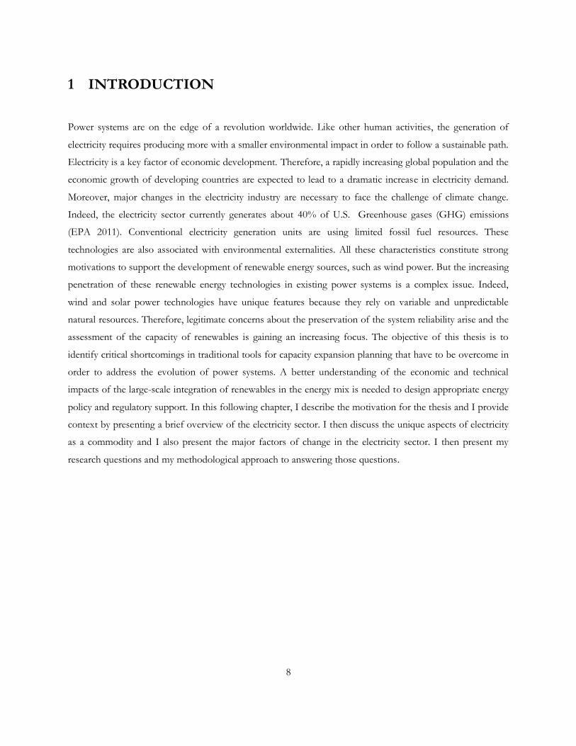
Since electricity is only marginally stored, electric generation plants are planned to withstand maximum power

load. For this reason, determining the chronological demand profile is critical to adequately supply electricity

in a system. For the same total energy consumed over a given period, different load profiles are met at

different costs. A relatively flat load curve is generally less expensive to supply than a spiked one because

ramping units are expensive to operate. Demand varies over timescales ranging from seconds to years. Over a

day, the load follows the pattern of a workday. Demand is typically higher during the workday, from 8am

until 7pm. The Figure 1 represents the hourly electricity demand for the U.S. during an average day in

January, April and June.

Figure 1. Electricity demand during a typical day, for different months (NREL 2006)

0

100

200

300

400

500

600

700

1 2 3 4 5 6 7 8 9 10 11 12 13 14 15 16 17 18 19 20 21 22 23 24

ho

url

y lo

ad i

n G

W

hours

hourly load in the U.S.

january april august

10

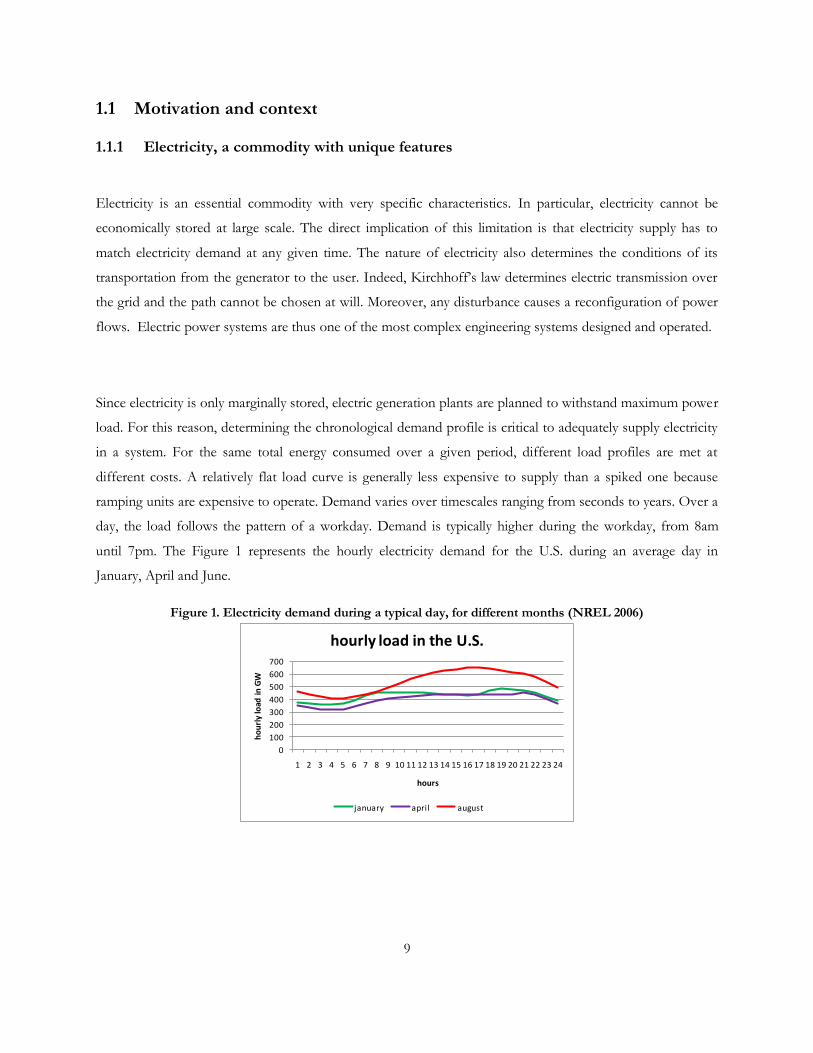
Over a week, the electricity demand follows the pattern of workdays and weekends. And finally over a year,

the demand has a seasonal pattern due to climate variations. Electricity demand is typically higher during

winter, due to high heating consumption, and during summer due to extensive air conditioning usage. The

Figure 2 represents the monthly electricity demand for the U.S. during a year.

Figure 2. Monthly electricity demand in the U.S. (NREL 2006)

0

50

100

150

200

250

300

350

400

450

1 2 3 4 5 6 7 8 9 10 11 12mo

nth

ly e

ne

rgy

de

man

d T

Wh

months

Monthly load for the U.S.

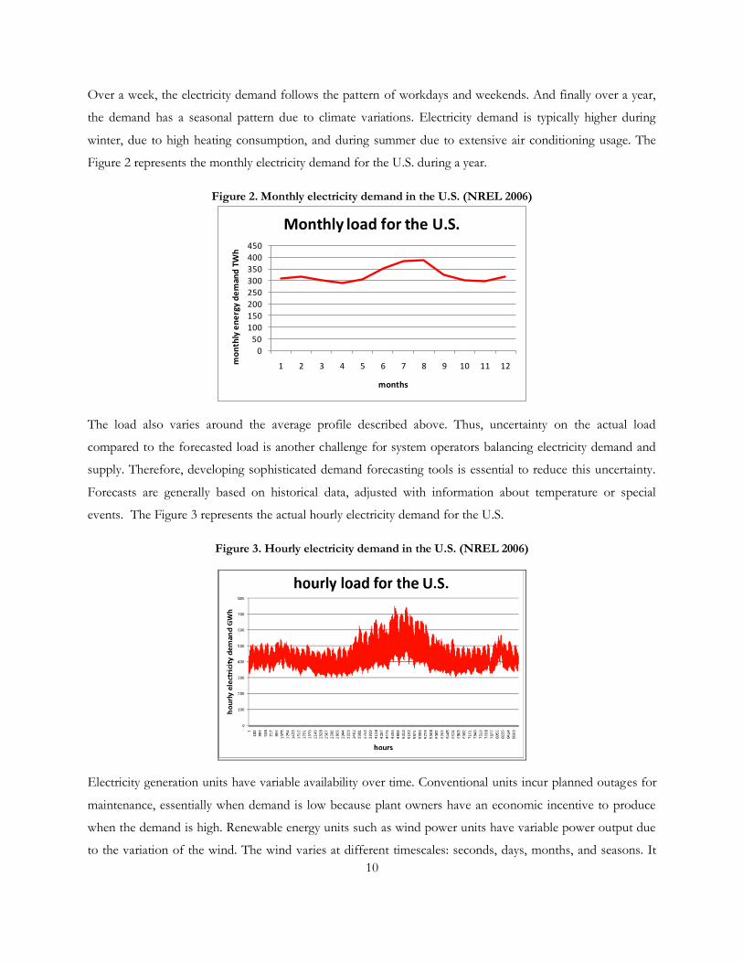
The load also varies around the average profile described above. Thus, uncertainty on the actual load

compared to the forecasted load is another challenge for system operators balancing electricity demand and

supply. Therefore, developing sophisticated demand forecasting tools is essential to reduce this uncertainty.

Forecasts are generally based on historical data, adjusted with information about temperature or special

events. The Figure 3 represents the actual hourly electricity demand for the U.S.

Figure 3. Hourly electricity demand in the U.S. (NREL 2006)

Electricity generation units have variable availability over time. Conventional units incur planned outages for

maintenance, essentially when demand is low because plant owners have an economic incentive to produce

when the demand is high. Renewable energy units such as wind power units have variable power output due

to the variation of the wind. The wind varies at different timescales: seconds, days, months, and seasons. It

11

also varies geographically, due to latitude, temperature, large-scale topography, small-scale site-specific

topography or built environment.

Moreover, there are different sources of uncertainty on the electricity supply-side. Conventional units suffer

unplanned forced outages, often due to mechanical problems. But the main source of uncertainty in the

electricity supply is the generation from renewable units. Indeed, the actual output from a wind plant varies

widely around the average wind profile. The uncertainty of the natural resource is not of a different nature

than the uncertainty of the forced outages for conventional units. However the frequency of non-availability

events is much larger for a wind power plant than for a conventional unit. Therefore, this uncertainty is often

considered as a key factor reducing the value of wind as a generation capacity, as I will discuss in the present

thesis.

1.1.2 Major factors of change in the electricity sector

Global population is expected to increase to nine billion in 2050, according to the 2008 World Population

Prospects of the United Nations (UN 2008). Developing countries with a large population such as China,

India or Brazil are rapidly increasing their electricity consumption per capita. Thus, electricity demand is

expected to boom. Moreover, the conventional fossil fuel technologies use limited natural resources and fuel

prices are likely to increase, as less accessible resources are extracted. Finally, a carbon policy may contribute

to rising fossil fuel prices.

The electricity sector represents 40% of the total GHG emissions in the U.S. (EPA 2011) and is consequently

required to change dramatically in the next decade. Among the different activities in the electricity sector, the

generation process emits the greatest amount of GHGs. Carbon dioxide (CO 2) is the major cause of climate

change and is a byproduct of coal, oil and gas combustion in steam plants. Coal plants are also emitting

Nitrous Oxide (NOx) and Sulphur Dioxide (SO 2), both having a large environmental impact. NOx and SO 2

are causing acid rains and NOx is also a major component in the formation of tropospheric ozone.

Conventional steam power plants are also responsible for heavy metals and particle emissions. While the

emissions caused by the nuclear energy are mainly due to the mining of the fossil fuels and the construction

period, the nuclear technology has also an uncertain but potentially large environmental impact. Indeed, the

production of nuclear waste from nuclear power plants is an unsolved issue and the risk of contamination by

nuclear particles is existing, though difficult to quantify. Technologies using renewable energy sources have a

12

lower carbon footprint than fossil-fuel technologies and are generally more environmentally friendly.

However, the environmental impact of renewables technologies is not zero. Hydroelectric power plants in

particular may greatly disturb the environment. All generation technologies have also a land and visual impact.

Methodologies such as Life Cycle Analysis are used to assess the environmental impact of one product from

its conception to its end of life (EPA 2006).

Sudden changes in power generated are difficult to absorb in current power systems due to the mechanical

inertia of conventional generators. By managing up and down reserves, system operators can match

fluctuating and uncertain demand. The minimum amount of reserves in a system depends on the generation

mix, the local weather pattern and the system interconnections. Indeed, a relatively isolated system requires

higher level of reserve than a much interconnected one. A significant increase in renewable energy

technologies is likely to increase the necessary reserves.

Demand-side management and efficiency in the electricity sector constitute other key factors of change. The

expression ―demand-side management‖ designates all techniques designed to rationalize consumption of

electric power. It is also associated with the notion of ―Smart grid‖, which has gained an increasing focus in

the last few years. It refers to a system where distributed generators are directly connected to distribution

networks and where digital technologies optimize the overall system operation. A rapid growth of distributed

generators is due to a favorable economic and regulatory context as well as a rationale for isolated location.

All these elements above add more complexity in the electric sector. Finally, the energy independence is

another factor to justify a diversification in the energy supply.

Due to the characteristics described above, the electricity supply has long been considered to be a public

service. In some cases, vertically integrated utilities were required to meet minimum quality standards and

their costs were covered by regulated prices, with reasonable rate of return. In other cases, such as in many

European countries until the nineties, electricity generation was nationalized. There have been changes

toward liberalization in many countries. The de-regulation that has changed many sectors of the economy

(telecommunications, aeronautics, etc.) has also impacted the electricity sector, leading to an increasing

competition between firms. Competition between generators became possible after the interconnection of

grids. Different areas of the electricity sector require various levels of centralized regulation. Indeed, the

transmission impacts generators competitiveness and has also been modified following the deregulation of

the electricity generation sector. However distribution has not been subjected to large changes. The

competition in electricity generation brought new challenges in the electricity sectors. Regulatory authorities

13

need to design market rules ensuring that profit maximization behaviors lead to the minimization of the

system costs. Utilities plan and operate to maximize their profit but are not responsible for the system

security. In a decentralized context, electricity firms are thus more exposed to risk, in theory, than in a

regulated market. Therefore the challenging issue of the wind power integration concerns all stakeholders in

power systems, including utilities.

1.2 Thesis Research Questions

These goals lead to the following more specific questions:

- What is the optimal electricity generation mix with large-scale integration of onshore wind power in

the long term?

- What are the economic impacts of the variability and the intermittency of the renewable energy

sources on power systems?

- What are the key features of a power system determining the cost of integrating renewables?

1.3 Methodology

To answer the research questions I have identified, I developed a cost minimizing static linear programming

model, CAPacity Expansion model with Wind variability (CAPEW), in the present thesis. It optimizes the

generation mix to supply variable demand during a year with conventional as well as wind power

technologies. I focus on the long term planning of the electricity generation capacity expansion in the U.S. to

illustrate the impact of the geographical diversity of U.S. regions. The CAPEW does not include the existing

installed units in order to find the optimal generation mix in a long-term time horizon without the constraints

of peculiar existing power systems. I focus on the integration of onshore wind power technology but future

explorations can include offshore wind power, solar power or other renewable sources.

14

1.4 Structure of the thesis

The chapters are organized as follows. Chapter one introduces my motivations and looks at the fundamental

features of electricity and reviews the major factors of change in the electricity sector. In this part, I also

present the methodology developed and I summarize the results of my analysis. In chapter two, I describe

the different modeling approaches at various timescales and I explore the methodologies used to integrate

wind power in traditional power system representations. I particularly focus on reliability measures and

capacity credit assessment. In chapter three, I present the static CAPacity Expansion model with Wind

variability (CAPEW) I developed for the purpose of the present analysis. Chapter four reviews the results of

the study. Finally in chapter five, I offer some conclusions and future possible extensions and I present the

implications of the result for the regulatory and policy design to support efficient wind power technology. .

15

2 INTEGRATING WIND IN THE REPRESENTATION OF

POWER SYSTEMS

2.1 Different timescales require different models

Utilities face both planning and operating decisions. For their part, regulators and investors need long-term

projections to support their decision process. At any decision level, sophisticated models provide forecasts

and assessments to help decisions-makers to optimize planning and operation activities. Different types of

models have been developed to help different stakeholders (utilities, system operators, regulators, policy

makers, etc.). In the long term, utilities design capacity expansion plans and secure fuel contracts. In the

medium term, they schedule facility maintenance and hydroelectric plant management. Finally, in the short

term, they operate capacity in reserve and connect generation units during the generation unit dispatch. For

long-term considerations, generation and transmission capacity expansion models have been developed.

Economic models with a broader scope are also particularly useful to capture interactions between sectors

decades ahead. Unit Commitment models are tools used for planning operation in the medium term, from

hours to a day ahead. This type of model integrates detailed technical aspects but does not include investment

considerations because of its limited time scope. Load forecasting and hydrothermal scheduling is done for a

day or a week. For the short term, minutes to hour ahead, economic dispatch and optimal power flow

models are used. In general, generating units are called to operate, or dispatched, in order of their increasing

operating costs, until demand is met, with some units kept in reserve. Optimal power flow models have the

advantage to account for transmission constraints. Finally operators use generation control and protection

models to ensure the stability of the system at very short term. In the Figure 4, different type of models are

represented as function of timescales and details level.

16

Figure 4. Different models at varying time scales

Economic Operation:-Economic dispatch-Optimal power flow

Unit Commitment

HydrothermalcoordinationLoad forecasting

- Generation and transmission capacity expansion- Economic Models

Seconds … Minutes … hours… days… weeks… years…

Generation controlProtection

not

det

aile

dve

ry d

etai

led

Long-term models are useful tools to provide insights into relative trends, as well as implications of various

policy measures. However the quantification from exploratory models does not take into account numerous

uncertainties. Thus these models, such as the capacity expansion model developed in this thesis, should only

be considered as imperfect tools helping discussion and illustrating key trade-offs.

2.2 Expansion planning

Generation expansion planning models optimize the capacity installed and the power generated in order to

meet demand at the lowest cost. Several parameters are considered to plan a generation capacity expansion in

a power system. The ratio of capital costs to operating costs is a key characteristic to determine the role of a

technology. To meet base load demand, capital-intensive plants with low operating costs are used. On the

contrary, peak demand is better served by ―peakers‖; plants, which are cheap to build but have high operating

costs. To build new generation units represents a large investment and requires long-term projections on the

performance of the plants over their lifetime. In a centralized system, the system operator uses expansion

planning models to design optimal future power systems. Expansion models are also tools used by regulators

to assess the economic and technical impacts of new regulations of power system. Finally, in a liberalized

market context, firms benefit from expansion planning models to maximize their profit. For long-term

decisions, technical details can be roughly approximated because of the high level of uncertainty. Different

approaches of generation planning are used, depending on the level of details needed: screening curve

methodology or detailed reliability analysis optimization.

17

2.2.1 Screening curve and the representation of wind power

The basic approach for expansion modeling is referred to as ―screening curves‖. It is a standard methodology

used to determine the optimal installed capacity to meet demand (Shaalan 2003; Kelly and Weinberg 1993). A

screening curve is a basic way to find the optimal generation mix of baseload, intermediate and peaking

capacities. It offers a sufficient representation when the time profile of load does not matter in first

approximation, as it is the case for dispatchable generations (Knight 1972; Stoft 2002). In this approach, load

is represented by a cumulative probability distribution during a year, referred to as a ―load duration curve‖.

Electricity demand is traditionally divided in three load periods from the longest to the shortest: base load,

shoulder and peak demand. The monotonic load curve represents the length of time that demand exceeds a

threshold. In the Figure 5 is represented the load duration curve from U.S. electricity demand in 2006. The

peak demand is found to be close to 650 GW and the total annual energy demand around 3 890 TWh.

Figure 5. Load duration curve for the U.S. (from NREL 2006)

0

100,000

200,000

300,000

400,000

500,000

600,000

700,000

0 1000 2000 3000 4000 5000 6000 7000 8000 9000 10000

load

in

MW

operating hours

Load duration curve for the U.S.

Figure 6. Screening curves (from EIA 2010 data)

-

10.00

20.00

30.00

40.00

50.00

60.00

70.00

0

40

0

80

0

1,2

00

1,6

00

2,0

00

2,4

00

2,8

00

3,2

00

3,6

00

4,0

00

4,4

00

4,8

00

5,2

00

5,6

00

6,0

00

6,4

00

6,8

00

7,2

00

7,6

00

8,0

00

8,4

00

8,7

60

Ave

rage

co

st (

$/M

Wh

)

operating hours

screening curves for conventional unitsreference costs scenario

pulverized_coal NGCC NGCC_CCS IGCC_CCS nuclear

18

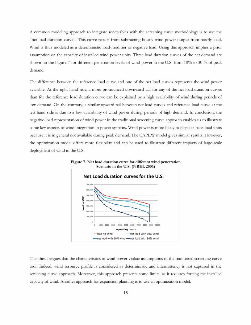
A common modeling approach to integrate renewables with the screening curve methodology is to use the

―net load duration curve‖. This curve results from subtracting hourly wind power output from hourly load.

Wind is thus modeled as a deterministic load-modifier or negative load. Using this approach implies a prior

assumption on the capacity of installed wind power units. Three load duration curves of the net demand are

shown in the Figure 7 for different penetration levels of wind power in the U.S. from 10% to 30 % of peak

demand.

The difference between the reference load curve and one of the net load curves represents the wind power

available. At the right hand side, a more pronounced downward tail for any of the net load duration curves

than for the reference load duration curve can be explained by a high availability of wind during periods of

low demand. On the contrary, a similar upward tail between net load curves and reference load curve at the

left hand side is due to a low availability of wind power during periods of high demand. In conclusion, the

negative-load representation of wind power in the traditional screening curve approach enables us to illustrate

some key aspects of wind integration in power systems. Wind power is more likely to displace base-load units

because it is in general not available during peak demand. The CAPEW model gives similar results. However,

the optimization model offers more flexibility and can be used to illustrate different impacts of large-scale

deployment of wind in the U.S.

Figure 7. Net load duration curve for different wind penetration Scenario in the U.S. (NREL 2006)

0

100,000

200,000

300,000

400,000

500,000

600,000

700,000

0 1000 2000 3000 4000 5000 6000 7000 8000 9000 10000

load

in

MW

operating hours

Net Load duration curves for the U.S.

load no wind net load with 10% wind

net load with 20% wind net load with 30% wind

This thesis argues that the characteristics of wind power violate assumptions of the traditional screening curve

tool. Indeed, wind resource profile is considered as deterministic and intermittency is not captured in the

screening curve approach. Moreover, this approach presents some limits, as it requires forcing the installed

capacity of wind. Another approach for expansion planning is to use an optimization model.

19

Wind power is classically also represented as a negative load in most optimization capacity expansion models.

In CAPEW, I consider wind power technology as any other technology except that wind availability is limited

by the hourly wind resource profile. Regional supply limitations of the wind resource are also added as a

constraint for each region and wind power class. This approach offers flexibility to incorporate uncertainty

and regional resource limitations. It also has the advantage to avoid forcing the installation of wind power

capacity.

2.2.2 Optimization of generation capacity expansion planning

Inputs in the capacity expansion model include variable costs (variable operation and maintenance or O&M,

heat rate, fuel prices), fixed costs (fixed O&M, capital costs), plant lifetime, carbon emissions and average

capacity factors. Technologies have different variable and fixed costs. To optimize the production of a certain

amount of electricity with different available technologies, the first criterion is to minimize the total cost to

meet a given demand. Decisions for generation and transmission expansion are based on forecasts of future

demand, fuel prices, technological evolution and regulation. Long term models are however usually based on

average constraints and do not generally include details necessary to capture the wind power intermittency

and variability. In short-term and real-time planning models the goal is to minimize actual generation cost

while maintaining the overall system reliability. Therefore, more details are taken into account. For example,

generation costs in Unit Commitment models include start-up and shut-down costs. Palmintier and Webster

offer an approach to combine the objective of long-term and real time-planning (Palmintier 2011).

There are multiple sources of uncertainty in an expansion-planning problem relating to:

Macroeconomic data (economic growth, electricity demand, fuel prices, etc.),

Technological innovations (costs reduction, efficiency, storage capacity, etc.),

Financial parameters (inflation, discount rate),

Climate evolution (temperature, solar irradiation, wind resource, hydrological reserves),

Technical characteristics of units (retirement assumptions of generators, building period, reliability),

Regulatory changes,

Public opposition or support for a technology, ect.

20

Many models do not represent these uncertainties and rely on long-term projections for relevant model

inputs.

2.2.3 The representation of wind power in capacity expansion optimization models

A standard indicator of the economic performance of electricity generation technologies is the Levelized Cost

of Electricity (LCOE). It measures the annualized total cost of a new generator over its lifetime in $/MWh

and is calculated by the ratio of the Net Present Value (NPV) of all costs divided by the amount of electricity

produced. The critical assumptions in a LCOE calculation are the investment cost (referred to as the

―overnight‖ cost), discount rates, financing options and capacity factor. In the LCOE, all costs are equally

allocated across all generated units. 1The LCOE appears to be inappropriate for renewables (Marcantonini

and Parsons, 2010). A key point to understand the debate over the value of electricity produced by renewable

technologies is that electricity is not a homogeneous good. Indeed some technologies produce base-load

power and are not flexible (such as nuclear plants), while others have the capacity to ramp quickly and

provide intermittent power (such as renewables).

A common approach to assess the economic value of the electricity produced by renewables is to associate a

back-up generating unit to a wind or solar power unit in order to get a more comparable dispatchable

resource (Morris, 2010). In this case, costs of renewable energy technologies are assessed in a worst-case

scenario. Indeed, this representation suggests that renewables need 100% back-up. But it has been

demonstrated that interconnection between wind turbines significantly reduces the no-wind case probability.

It is then reasonable to assume that a relevant back-up amount should be less than 100%. However,

determining a back-up quantity still lies upon the hypothesis than renewable compete on the base-load power

generation.

1 Therefore this approach implicitly implies that the evaluated generation technology produces base-load power and can be dispatched. Indeed, the amount of energy produced in the LCOE is calculated as the product of the installed capacity and the average capacity factor. This annual average capacity factor depends on the natural resource and thus on the location of the plant.

21

2.2.4 ReEDS model

The National Renewable Energy Laboratory (NREL) has developed a model called ReEDS (Regional Energy

Deployment System), in order to study the expansion of generation and transmission capacity in the U.S.

electricity sector. ReEDS (Short 2003; Short et. al. 2009) is a recursive-dynamic capacity expansion and

dispatch linear programming model.

In addition to the standard technical constraints taken into account to minimize total system cost (meeting

demand, reserve requirements, regional resource supply limitations and transmission constraints), ReEDS

includes state and federal policy requirements and national renewable requirements (e.g. a national 80% RE-

by-2050 target). The optimization and dispatch occurs every two years from the start period to 2050. Every

period is divided in 17 time slices to represent the seasonal and diurnal variation in demand and resource

profile (morning, afternoon and night for every season and a ―peak‖ slice in the summer). The planning and

operating reserve requirements are then satisfied in all time slices.

Among capacity expansion models, ReEDS differentiates by its high regional discretized structure and

statistical treatment of the impact of variability. This methodology is intended to capture location-dependent

quality of natural resources. Moreover, the detailed regional and temporal representation enables ReEDS to

consider the cost of transmission expansion. Using hourly data, standard deviations of power output are

calculated during each time slices for each wind power class and region. This calculation relies on the

geographically aggregated variability in each reserve-sharing region. Correlation statistics are also included in

standard deviations to reflect the smoothing of variability from geographically dispersed wind turbines. It is

assumed that the degree of positive correlation between turbines is higher for turbines located in the same

area, which increases the standard deviation. One key assumption is also than the profiles of load and wind

resource are uncorrelated. CAPEW does not include transmission constraints and statistical treatment of the

variability of the natural resources. However, its structure also captures the location-dependent quality of the

wind resource and the correlation between temporal variation of the load and the wind resource.

22

2.2.5 Power system reliability measures

Conventional units such as coal-fired and gas-fired turbines are dispatchable, meaning that they can be turned

on or off upon demand. For this reason, conventional units can count their full capacity, minus an average

forced outage rate, toward the planning of reserve requirement. On the contrary, renewable energy

technologies are not dispatchable and cannot count their full capacity, minus an average ―no-resource‖ rate

toward the planning of reserve requirement because their availability is variable. The capacity value can be

defined as the fraction of the total capacity, which can reliably count toward the long term planning of reserve

requirement. This capacity value is commonly estimated with the effective load carrying capacity (ELCC).

Different operating reserve requirements are commonly distinguished by their timescales. The timescale

necessary for a generator to change its output defines its flexibility. Generators constitute spinning reserves if

they are not producing at full capacity but can ―ramp-up‖ quickly (e.g. in less than 10 minutes) on a given

capacity amount. ―Quick start‖ reserves are provided by technologies able to start up in less than minutes,

such as natural gas combustion turbines. Interruptible load can also be considered as a demand-side reserve

requirement option. Contingency reserve requirement ensures that the system will adapt to an unforeseen

change in generation or transmission, typically due to outages at a 10-minutes timescale. Both spinning and

interruptible load are considered as contingency reserves. The frequency regulation reserve requirement deals

with sub-minute deviation between electricity demand and supply. There is no standard approach to

determine required level of operating reserves. In some NERC areas (North American Electric Reliability

Corporation), the operating reserve is at least as large as the largest single system. In others, the operating

reserve is typically around 7% if the peak demand and lower if hydro is serving a large share of the demand

(NERC). This level of detail in operating reserves described above is not included in the CAPEW model but

a reserve margin of 10% is modeled.

23

Stochastic reliability assessment methodologies using probabilities to represent uncertainty are briefly

described below. The LOLP is a measure of the probability of inadequacy of the electricity generation to

serve the load. It is calculated from the hourly load levels, the generation capacity and the forced outage rates.

This reliability measure can also be expressed through the Loss Of Load Expectation (LOLE). It represents

the number of hours per day, days per years or days during ten years, during which the load might not be

served. A standard target LOLP level is one day in ten years. In reliability models, forced outages rates reflect

equipment malfunctions or other unplanned events for conventional units. Similarly, the availability of a wind

plant can be captured in a forced outage rate taking into account the intermittency of the wind. This rate will

derive from the probability distribution of the wind speed.

The statistical Effective Load Carrying Capability (ELCC) is generally calculated in order to evaluate the

capacity value of a technology. It represents the amount of electricity demand that may be added in each time

slice for an incremental increase of the capacity in a given technology, without any increase in the LLOP, as

defined below. In other words, the ELCC represents the share of available capacity for one incremental unit

of installed capacity at a constant reliability level of the system. In order to capture the magnitude of the

energy not served, the Expected Energy Not Served (EENS) is also calculated. It represents the amount of

energy that has to be curtailed. (Chowdhury 2003)

2.2.6 Average capacity versus Firm Capacity

The debate about the cost of integrating renewables is embedded in the question of the power system

reliability and the plant‘s capacity value of renewable technologies. Determining the capacity credit of wind is

important from an operational perspective. But it also matters from an economic standpoint because it

changes the economic value of wind from the utility‘s point of view. Therefore, a clear definition of the term

―capacity‖ is essential. The average availability is defined as the average power production that can be

sustained permanently over a period of a year. For conventional technologies, this average availability

depends essentially on the technical availability of generators. However, for the wind power technology, the

average availability also largely depends on the wind resource. This average availability is commonly called

annual capacity factor. It is calculated by the ratio of the expected power output divided by the annual rated

output. Average capacity factors are useful in terms of planning to estimate production on the long-term. But

this number alone does not capture the value of wind in a system. For example if the wind resource profile is

negatively correlated with the system load profile, the wind capacity factor during peak will be lower than the

annual capacity factor. And on the contrary, if the wind resource profile is positively correlated with the load

24

profile, the wind capacity factor during the peak demand period will be higher than the annual average

capacity factor.

In term of operations, the priority is to avoid a loss of load. Therefore the focus is on the peak hours when

most generation units installed are operating. The firm capacity, also called capacity credit or load

carrying capability, is the readiness to operate during high demand or emergencies. Firm capacity is

expressed as a fraction of the total installed capacity. For renewables, the term ‗capacity credit‘ is generally

used to refer to the magnitude of the conventional units capacity that can be displaced by a unit of capacity

from these renewables. The firm capacity is generally higher than the average availability for conventional

technologies because of economic incentives for plant owners to operate during peak times. On the contrary,

the firm capacity is generally lower than the average availability for wind power plants because wind power

technology is not dispatchable and plant owners cannot choose to produce during peak hours if the wind is

not blowing.

To conclude, the average capacity factor, or availability, of a wind plant depends on the wind quantity while

the firm capacity, or capacity credit, depends on the adequacy of the wind resource, given a load profile (i.e.

the wind plant production during peak demand). Some studies argue that arrays of wind farm produce some

firm capacity because of the diversity of wind at geographical dispersed sites. (Chowdhury 1991).

25

3 CAPEW, A CAPACITY EXPANSION MODEL WITH WIND

VARIABILITY

3.1 Objectives of the model

The integration of the renewables1 is a chicken-and-egg problem in the sense that the initial design of power

systems with conventional technologies makes the increase of the share of renewables costly, but this increase

is also likely to modify the structure of the power systems and lower integration costs in the future. The

objective of the CAPEW model is to tackle this issue and to offer an answer to the question of the optimal

generation mix, given the available technologies and the variability and intermittency of wind power.

3.2 Hypothesis

CAPEW is a linear program minimizing the power system total cost subject to basic constraints: meeting

demand, reserve requirements and regional resource supply limitations. CAPEW is a static electricity

generation capacity expansion model developed in a centralized planning context. Indeed the cost

minimization formulation is coherent in a context of cost of service remuneration2. Different cost minimizing

optimization models represent wind variability by modeling wind as a negative demand (De Jongue et al.

2010). This approach necessitates a prior assumption on the installed capacity of wind and does not enable to

differentiate between power class resources. It also lacks the chronological description of wind and load

profile by using load duration curves, and thus does not allow capturing the correlation effect between load

and wind resource profiles. In order to illustrate the impact of the variety of the regional wind resource in

term of quantity and adequacy, a different and innovative approach is taken in the CAPEW model. More

specifically, wind power is modeled as any other technology but its non-dispatchable characteristic is

represented by a variable cap on the generated electricity profile as a percentage of the installed wind capacity.

For the sake of simplicity, I also assume that all the revenues come from the sale of electricity, neglecting

ancillary services or remuneration for providing capacity. Some operational aspects, as start-up costs,

1 The focus of the model is on wind, but future extension include the integration of other renewable source technologies

2 To consider a decentralized approach, the objective function of the model has to be the maximization of firms‘ profit.

26

minimum operating level, minimum up and down times introduce binary variables. It requires using a mixed

integer linear programming (MILP) formulation. Solving a MILP problem poses some computational

difficulties for a one-year dataset. For these reasons, these operational constraints are not considered in

CAPEW. Transmission constraints are also not considered and no storage capacity is included in the system.

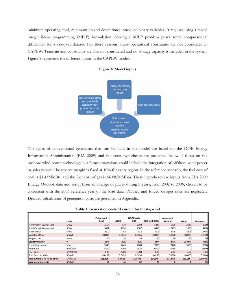
Figure 8 represents the different inputs in the CAPEW model.

Figure 8. Model inputs

Optimization:

Optimal installed capacity

Optimal hourly generation

Hourly wind data and available capacity per

power class per region

Hourly electricity demand per

region

Generation costs

The types of conventional generators that can be built in the model are based on the DOE Energy

Information Administration (EIA 2009) and the costs hypotheses are presented below. I focus on the

onshore wind power technology but future extensions could include the integration of offshore wind power

or solar power. The reserve margin is fixed at 10% for every region. In the reference scenario, the fuel cost of

coal is $1.4/MMBtu and the fuel cost of gas is $6.08/MMBtu. These hypotheses are inputs from EIA 2009

Energy Outlook data and result from an average of prices during 5 years, from 2002 to 2006, chosen to be

consistent with the 2006 reference year of the load data. Planned and forced outages rates are neglected.

Detailed calculations of generation costs are presented in Appendix.

Table 1. Generation costs S1 current fuel costs, wind

Units

Pulverized

Coal NGCC

NGCC with

CCS IGCC with CCS

Advanced

Nuclear Wind Biomass

"Overnight" Capital Cost $/kW 3167 978 2060 5348 5335 2438 3860

Total Capital Requirement $/kW 3674 1056 2307 6418 7469 2633 4478

Fixed O&M $/kW 36.0 14.4 30.3 69.3 88.8 28.1 100.5

Variable O&M $/kWh 0.0043 0.0034 0.0065 0.0080 0.0020 0.0000 0.0050

Project Life years 20 20 20 20 20 20 20

Capacity Factor % 85% 85% 80% 80% 85% 32-46% 80%

Operating Hours hours 7446 7446 7008 7008 7446 3066 7008

Heat Rate BTU/kWh 8800 7050 7525 10700 10488 0 13500

Fuel Cost $/MMBTU 1.40 6.08 6.08 1.40 0.63 0.00 1.03

Fuel Cost per kWh $/kWh 0.0123 0.0429 0.0458 0.0150 0.0066 0.0000 0.0140

total annualized fixed costs $/MW-yr 185,485 53,532 116,873 324,345 377,888 133,056 228,905

total variable costs $/MWh 17 46 52 23 9 0 19

27

3.3 Model Structure

3.3.1 Objective Function

The model optimizes the total cost of expansion and operation of the power system. Total system cost is

defined as the sum of total variable cost and total fixed cost.

TC= TCvar + TCfix

- TC is the total system cost ($)

- TCvar is the total variable cost ($)

- TCfix is the total fixed costs ($).

3.3.2 Equations

The total fixed cost is the sum of all the installed capacity multiplied by their annualized fixed cost.

TCfix = c_fix(G)* InsCap(G,r)

- c_fix (G) is the annualized fixed cost for the technology G ($/MW-year)

- InsCap (G,r) is the total installed capacity of units of the technology G, in the region r (MW)

- TCfix is the total fixed costs ($).

The variable cost is the sum of the energy generated multiplied by the variable generation cost. The hourly

energy generation is equivalent to the instantaneous power, averaged over a time step of one hour.

TCvar = c_var(G)* PwrOut(h,G,r)

- c_var (G) is the variable generation cost ($/MWh)

- PwrOut (h,G,r) is the power available during an hour, for the technology G in the region r (MW) and

is equivalent to the hourly energy generated during an hour.

- TCvar is the total variable cost ($).

28

3.3.3 Constraints

Supply has to meet demand

The power generated during an hour in the region r has to be equal to the sum of the demand and an

operating reserve margin1.

PwrOut (h,G,r) = load (h,r) * (1+r)

- r is the reserve margin %

- load (h,r) is the electricity demand during the hour h in the region r (MWh)

- PwrOut (h,G,r) is the power produced during the hour h, by technology G in the region r (MW)

Electricity generated by conventional units

The power generated by each type of conventional technology G* is limited by the available capacity defined

as the product of the installed capacity and the annual average capacity factor.

PwrOut (h,G*,r) ≤ InsCap(G*,r)*CF(G*)

- PwrOut (h,G*,r) is the power produced during the hour h, by the conventional technology G* in the

region r (MW)

- InsCap (G*,r) is the total installed capacity of units of the conventional technology G*, in the region

r (MW)

- CF (G*) is the annual average capacity factor of the conventional technology G*

Electricity generated by wind power units:

The power generated by wind plants is limited by the available capacity, defined as the product of the installed

capacity, the capacity factor and the variable wind resource profile. The wind power technology is represented

by five distinct technologies in the model, from class 3 to class 7, indexed by ―wind i‖, I = 3, …, 7.

1 The planning reserve margin r required by system planners represents generally 12-20% of the peak load margin of extra capacity (Holttinen 2008), the value chosen in CAPEW is 10%

29

PwrOut (h,wind i,r) ≤ InsCap( wind i, r)*CF (wind i)*wind_profile(h,r)

- PwrOut (h,wind i,r) is the power produced during the hour h, by wind power of class i in the region r

(MW)

- InsCap (wind i,r) is the total installed capacity of units of the wind of class i, in the region r (MW)

- CF (wind i) is the capacity factor of the wind of class power i

- Wind_profile (h, r) is the wind profile by hour and region (%).

Installed wind capacity:

The installed capacity of wind power units for each wind power class is limited by the available capacity by

region derived from land requirements.

InsCap (wind i,r) ≤ MaxWind(wind i,r)

- InsCap (wind i,r) is the total installed capacity of units for the wind power class i, in the region r

(MW)

- MaxWind (wind i, r) is the maximum available capacity by region and wind power class derived from

the regional resource supply function.

The nuclear plants are operating at full capacity

The power produced by the nuclear plants is considered to be equal to the installed capacity times the

capacity factor to represent the absence of flexibility in the operation of nuclear plants.

PwrOut(h,nuclear,r) ≥ InsCap(nuclear, r)*CF(nuclear)

- InsCap (nuclear,r) is the total installed capacity of nuclear, in the region r (MW)

- CF (nuclear) is the capacity factor of nuclear plants

- PwrOut (h,nuclear,r) is the power produced during the hour h, by nuclear power plants in the region

r (MW).

30

3.4 Data

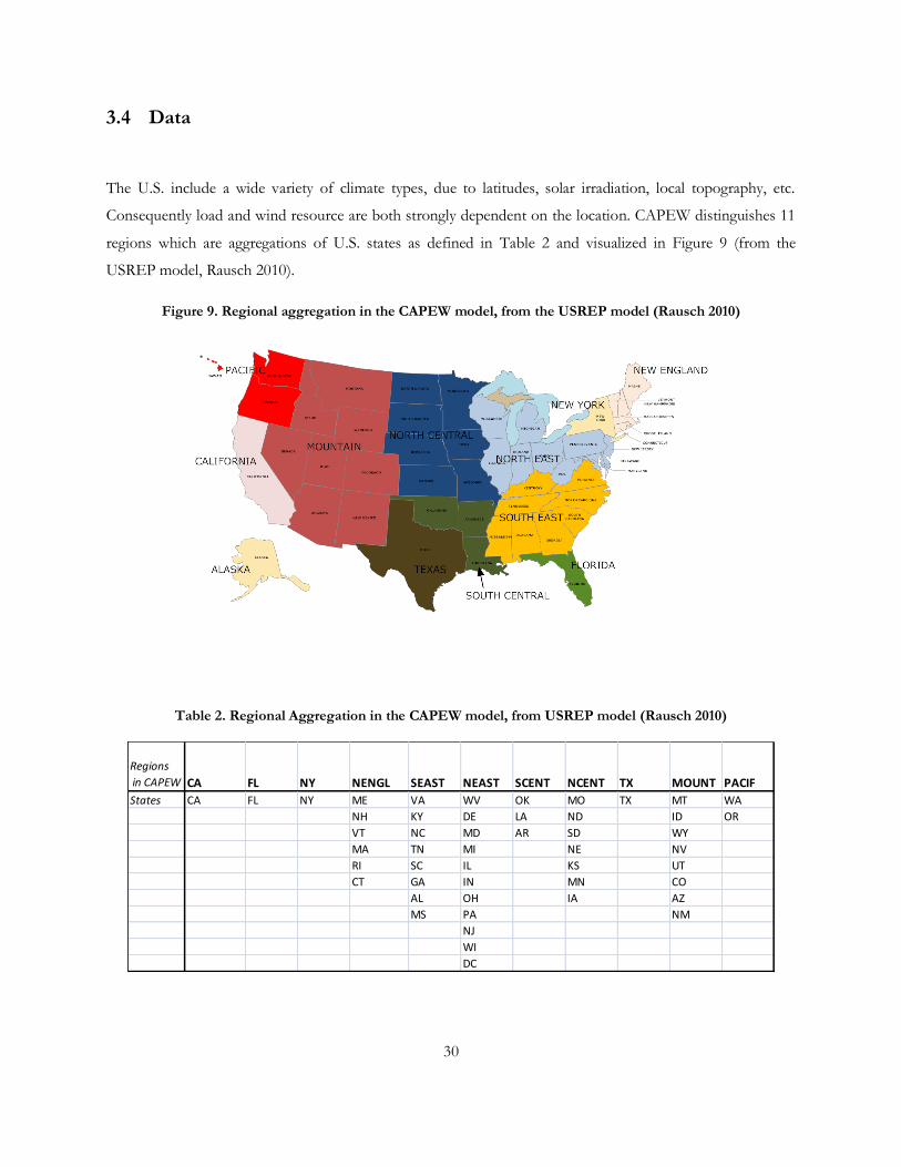
The U.S. include a wide variety of climate types, due to latitudes, solar irradiation, local topography, etc.

Consequently load and wind resource are both strongly dependent on the location. CAPEW distinguishes 11

regions which are aggregations of U.S. states as defined in Table 2 and visualized in Figure 9 (from the

USREP model, Rausch 2010).

Figure 9. Regional aggregation in the CAPEW model, from the USREP model (Rausch 2010)

Table 2. Regional Aggregation in the CAPEW model, from USREP model (Rausch 2010)

Regions

in CAPEW CA FL NY NENGL SEAST NEAST SCENT NCENT TX MOUNT PACIF

States CA FL NY ME VA WV OK MO TX MT WA

NH KY DE LA ND ID OR

VT NC MD AR SD WY

MA TN MI NE NV

RI SC IL KS UT

CT GA IN MN CO

AL OH IA AZ

MS PA NM

NJ

WI

DC

31

Hourly load and hourly wind resource in CAPEW are aggregated over 720 time slices within each year: twelve

months, each with twenty-four hours to illustrate a typical day. The optimization is done with a constraint of

meeting the load during each of the 720 periods and in each of the 11 regions. These time slices allow

CAPEW to capture the intricacies of meeting peak demand for electricity generators.

3.4.1 Load data

The database used in CAPEW consists of hourly electricity demand for the year 2006 in the 356 U.S. regions

defined in the ReEDS model. The high geographic and temporal resolution enables the model to capture

seasonal and daily variability of the load. The optimization in CAPEW is done for each time slice and each

region as defined above in order to capture temporal and geographical patterns. By representing the yearly

pattern of the electricity demand, differences between the eleven regions of CAPEW appear. In particular, the

―PACIF‖ region, including the states of Oregon and Washington, has a very distinct yearly load profile from

the other states. Indeed, the load demand is quite flat and does not include a peak in summer.

3.4.2 Wind resource profile

The United States possesses abundant wind resources. I consider five wind power classes based on wind

speed at 50 meters above ground and wind power density, ranging from Class 3 to Class 7, as defined in the

Table 3. Wind power classesTable 3.

Table 3. Wind power classes

wind power class

wind power density (W/m^2)

speed (m/s)

3 300-400 6.4-7.0 4 400-500 7.0-7.5 5 500-600 7.5-8.0 6 600-800 8.0-8.8 7 >800 >8.8

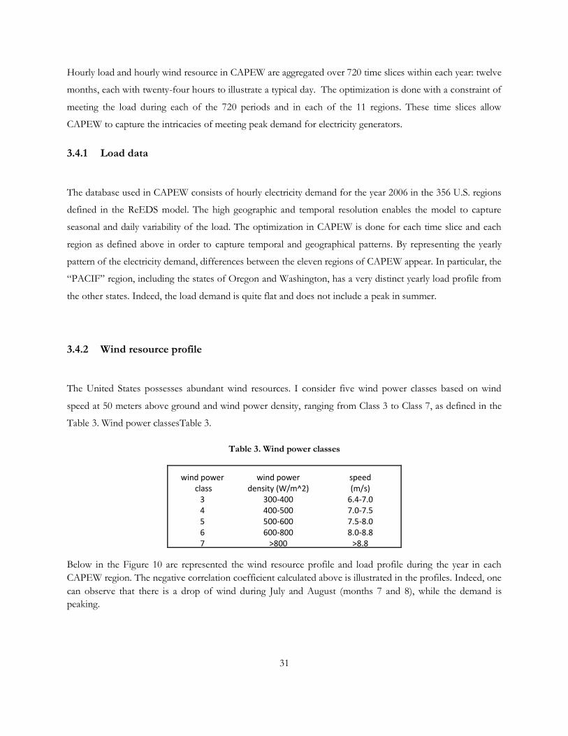
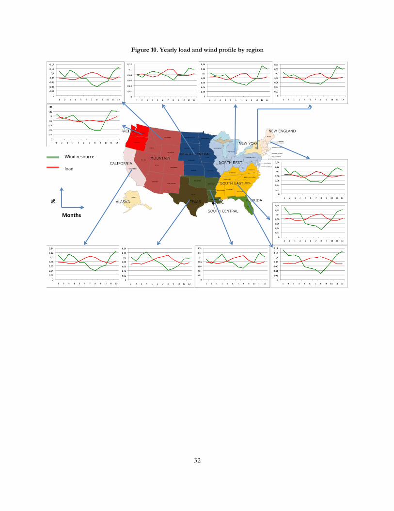
Below in the Figure 10 are represented the wind resource profile and load profile during the year in each

CAPEW region. The negative correlation coefficient calculated above is illustrated in the profiles. Indeed, one

can observe that there is a drop of wind during July and August (months 7 and 8), while the demand is

peaking.

32

Figure 10. Yearly load and wind profile by region

Wind resource

load

Months

%

33

The available land area per wind class has been derived from wind resource maps, after the exclusion of used

land and protected area in the NREL dataset. A constant multiplier of 5MW/km2 has then been applied to

convert available land into available wind capacity. The available wind capacity by region and wind power

class is plotted in regional wind supply curves in the Figure 11.

Figure 11. Wind available per power class

Available wind capacity (MW)

Win

d p

ow

er

clas

s

34

3.4.3 The adequacy of the wind resource

From hourly wind resource profile and hourly load profile, I calculate a ‗correlation coefficient‘. Correlation is

a measure of the strength and direction of a linear relationship between two datasets, here the wind resource

(w) and the load (l). Pearson‘s product moment correlation coefficient (Moore 1995) r is given by:

i i

ii

i

ii

llww

llww

lwr22

),(

Where l and w are the sample means of l and w.

All the regional load profiles, except for the region ―PACIF‖ are negatively correlated with the wind resource

profiles. This result can be related to the shape of the net load duration curves described above. Indeed, these

negative coefficients of correlation are an illustration of the fact that there is generally less wind when the

demand is higher. Below, the regional coefficients of correlation are calculated between hourly load profile

and hourly wind profile, and listed for each region defined in CAPEW.

Figure 12. Coefficient of correlation between the load and the wind profiles

region

correlation coefficient

betwen load and wind

profiles

CA -0.573

FL -0.745

NY -0.500

NENGL -0.567

SEAST -0.609

NEAST -0.555

SCENT -0.756

NCENT -0.679

TX -0.706

MOUNT -0.617

PACIF 0.259

US -0.722

35

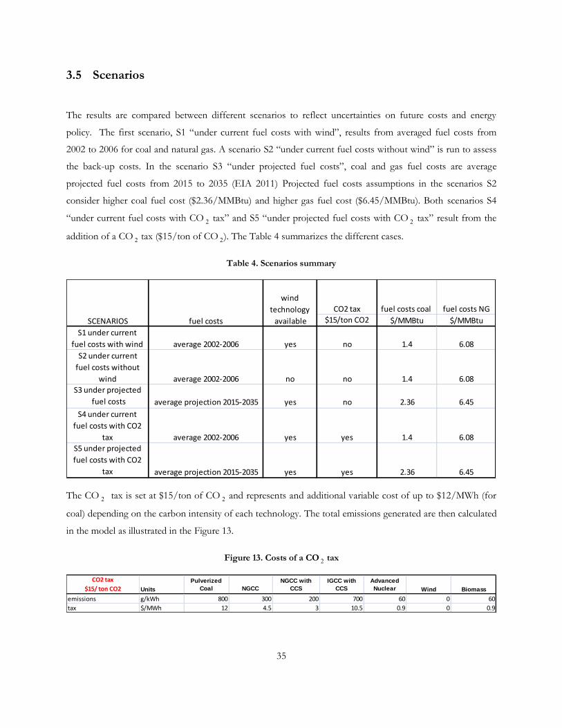
3.5 Scenarios

The results are compared between different scenarios to reflect uncertainties on future costs and energy

policy. The first scenario, S1 ―under current fuel costs with wind‖, results from averaged fuel costs from

2002 to 2006 for coal and natural gas. A scenario S2 ―under current fuel costs without wind‖ is run to assess

the back-up costs. In the scenario S3 ―under projected fuel costs‖, coal and gas fuel costs are average

projected fuel costs from 2015 to 2035 (EIA 2011) Projected fuel costs assumptions in the scenarios S2

consider higher coal fuel cost ($2.36/MMBtu) and higher gas fuel cost ($6.45/MMBtu). Both scenarios S4

―under current fuel costs with CO 2 tax‖ and S5 ―under projected fuel costs with CO 2 tax‖ result from the

addition of a CO 2 tax ($15/ton of CO 2). The Table 4 summarizes the different cases.

Table 4. Scenarios summary

CO2 tax fuel costs coal fuel costs NG

$15/ton CO2 $/MMBtu $/MMBtu

S1 under current

fuel costs with wind average 2002-2006 yes no 1.4 6.08

S2 under current

fuel costs without

wind average 2002-2006 no no 1.4 6.08

S3 under projected

fuel costs average projection 2015-2035 yes no 2.36 6.45

S4 under current

fuel costs with CO2

tax average 2002-2006 yes yes 1.4 6.08

S5 under projected

fuel costs with CO2

tax average projection 2015-2035 yes yes 2.36 6.45

SCENARIOS fuel costs

wind

technology

available

The CO 2 tax is set at $15/ton of CO 2 and represents and additional variable cost of up to $12/MWh (for

coal) depending on the carbon intensity of each technology. The total emissions generated are then calculated

in the model as illustrated in the Figure 13.

Figure 13. Costs of a CO 2 tax

CO2 tax

$15/ ton CO2 Units

Pulverized

Coal NGCC

NGCC with

CCS

IGCC with

CCS

Advanced


emissions g/kWh 800 300 200 700 60 0 60

tax $/MWh 12 4.5 3 10.5 0.9 0 0.9

36

4 RESULTS

4.1 S1 “under current fuel costs with wind power”

In the S1 scenario ―under current fuel costs with wind power‖, wind technology is available. The fuel costs

are 1.4$/MMBtu for coal and 6.08$/MMBtu for natural gas. These hypotheses are inputs from EIA 2009

Energy Outlook data and result from an average of prices during 5 years, from 2002 to 2006, chosen to be

consistent with the 2006 reference year of the load data (EIA 2009).

It is found that the coal-fired units represent 52% of the installed capacity on average in the U.S. The

remaining of the generation mix is composed of wind power units and natural gas-fire units. Nuclear

technology is not included in the generation mix. One explanation for this is that the operating constraint

formulated in the model for nuclear plants allows no flexibility in the operation of the plant. Consequently, it

increases the costs of nuclear technology compared to other technologies. In order to identify the role of the

wind power technology in the simulated power system, I compare the S1 scenario ―under current fuel costs

with wind power‖ and the S2 scenarios ―under current fuel costs without wind power‖, where wind power

technology is not available. As illustrated in the Figure 14 and Figure 14, wind power displaces coal

technology. Indeed, coal-fired units represent only 52% of the installed capacity on average in the U.S. when

wind power is introduced. But they represent almost 58% of the installed capacity if wind power technology

is not available.

Figure 14. Installed capacity (%) S1 “under current fuel costs with wind power”

0%

10%

20%

30%

40%

50%

60%

70%

80%

CA FL NY NENGL SEAST NEAST SCENT NCENT TX MOUNT PACIF

inst

alle

d c

apac

ity

%

Generation mix reference case

pulverized_coal

NGCC

wind4

wind5

wind6

wind7

37

Figure 15. Installed capacity (%) S2 “under current fuel costs without wind power”

0%

10%

20%

30%

40%

50%

60%

70%

80%


inst

alle

d c

apac

ity

%

generation mix, reference case, no wind power

pulverized_coal

NGCC

I also represent in the figure below the installed capacity for each region to illustrate the various sizes of the power

systems considered.

Figure 16. Installed capacity (MW) S1 “under current fuel costs with wind power”

0

20000

40000

60000

80000

100000

120000

140000

160000


inst

alle

d c

apac

ity

MW

Generation mix reference case

pulverized_coal

NGCC

wind4

wind5

wind6

wind7

Natural gas-fired units serve as reserves units in the system to handle both load and wind resource variability.

I calculate the actual capacity factor of the installed gas-fired plants as a ratio of the actual energy generated to

the installed capacity. This indicator ranges from 15 to 20% in the different regions. The gas-fired plants are

used with an average capacity factor of 17% in the U.S. due to the high variable cost.

38

Table 5. Operation of gas-fired units with and without wind

scenarios

S1 ―under current fuel

costs with wind power‖

S2 ―under current fuel

costs without wind power‖

Regions Average actual capacity factor

of the installed gas-fired units

Average actual capacity factor

of the installed gas-fired units

CA 15% 28%

NY 18% 36%

NENGL 19% 38%

SEAST 16% 27%

NEAST 15% 27%

SCENT 17% 26%

NCENT 18% 30%

TX 18% 27%

MOUNT 18% 29%

PACIF 23% 38%

average US 17% 31%

Wind power integration varies widely across regions (from 0 to 22%). The total wind power installed capacity

is 49GW1, representing 5% of the total installed capacity in the U.S.

Figure 17. Integration of wind per region, S1 “under current fuel costs with wind power”

0.0%

5.0%

10.0%

15.0%

20.0%

25.0%

CA FL NY

NEN

GL

SEA

ST

NEA

ST

SCEN

T

NC

ENT TX

MO

UN

T

PA

CIF

% o

f in

stal

led

cap

acit

y

integration of wind

% total installed capacity

Table 6. Integration of wind per region, S1 “under current fuel costs with wind

power”

integration of wind power CA FL NY NENGL SEAST NEAST SCENT NCENT TX MOUNT PACIF US

% total installed capacity 8.73% 0.00% 0.72% 7.01% 0.00% 0.13% 0.00% 21.87% 0.02% 20.76% 22.55% 5.5%

1 The current wind power installed capacity in the U.S. is around 40GW.

39

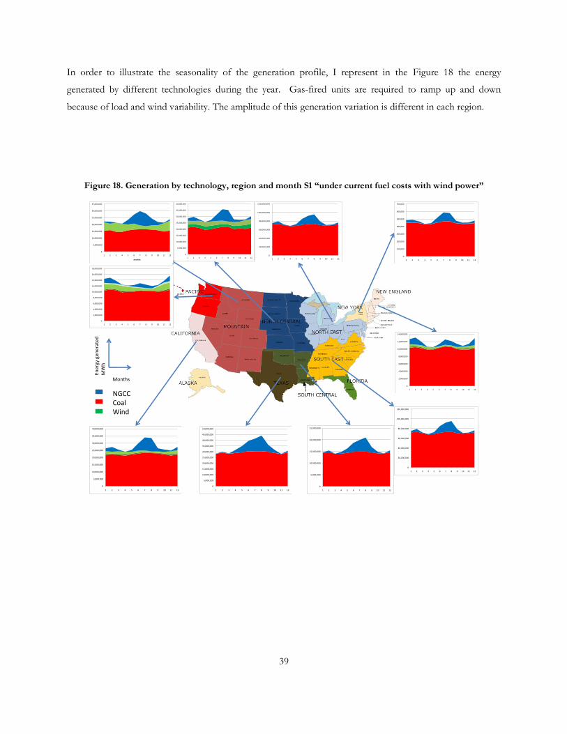
In order to illustrate the seasonality of the generation profile, I represent in the Figure 18 the energy

generated by different technologies during the year. Gas-fired units are required to ramp up and down

because of load and wind variability. The amplitude of this generation variation is different in each region.

Figure 18. Generation by technology, region and month S1 “under current fuel costs with wind power”

Months

Ener

gy g

ener

ated

M

Wh

0

5,000,000

10,000,000

15,000,000

20,000,000

25,000,000

30,000,000

35,000,000

1 2 3 4 5 6 7 8 9 10 11 12

months

0

2,000,000

4,000,000

6,000,000

8,000,000

10,000,000

12,000,000

14,000,000

16,000,000

18,000,000

1 2 3 4 5 6 7 8 9 10 11 12

0

5,000,000

10,000,000

15,000,000

20,000,000

25,000,000

30,000,000

35,000,000

40,000,000

1 2 3 4 5 6 7 8 9 10 11 120

20,000,000

40,000,000

60,000,000

80,000,000

100,000,000

120,000,000

1 2 3 4 5 6 7 8 9 10 11 120

100,000

200,000

300,000

400,000

500,000

600,000

700,000

1 2 3 4 5 6 7 8 9 10 11 12

0

2,000,000

4,000,000

6,000,000

8,000,000

10,000,000

12,000,000

14,000,000

1 2 3 4 5 6 7 8 9 10 11 12

0

20,000,000

40,000,000

60,000,000

80,000,000

100,000,000

120,000,000

1 2 3 4 5 6 7 8 9 10 11 12

0

5,000,000

10,000,000

15,000,000

20,000,000

25,000,000

1 2 3 4 5 6 7 8 9 10 11 12

0

5,000,000

10,000,000

15,000,000

20,000,000

25,000,000

30,000,000

35,000,000

40,000,000

45,000,000

50,000,000

1 2 3 4 5 6 7 8 9 10 11 12

0

5,000,000

10,000,000

15,000,000

20,000,000

25,000,000

30,000,000

35,000,000

40,000,000

1 2 3 4 5 6 7 8 9 10 11 12

NGCCCoalWind

40

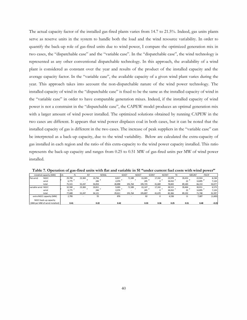
The actual capacity factor of the installed gas-fired plants varies from 14.7 to 21.5%. Indeed, gas units plants

serve as reserve units in the system to handle both the load and the wind resource variability. In order to

quantify the back-up role of gas-fired units due to wind power, I compare the optimized generation mix in

two cases, the ―dispatchable case‖ and the ―variable case‖. In the ―dispatchable case‖, the wind technology is

represented as any other conventional dispatchable technology. In this approach, the availability of a wind

plant is considered as constant over the year and results of the product of the installed capacity and the

average capacity factor. In the ―variable case‖, the available capacity of a given wind plant varies during the

year. This approach takes into account the non-dispatchable nature of the wind power technology. The

installed capacity of wind in the ―dispatchable case‖ is fixed to be the same as the installed capacity of wind in

the ―variable case‖ in order to have comparable generation mixes. Indeed, if the installed capacity of wind

power is not a constraint in the ―dispatchable case‖, the CAPEW model produces an optimal generation mix

with a larger amount of wind power installed. The optimized solutions obtained by running CAPEW in the

two cases are different. It appears that wind power displaces coal in both cases, but it can be noted that the

installed capacity of gas is different in the two cases. The increase of peak suppliers in the ―variable case‖ can

be interpreted as a back-up capacity, due to the wind variability. Below are calculated the extra-capacity of

gas installed in each region and the ratio of this extra-capacity to the wind power capacity installed. This ratio

represents the back-up capacity and ranges from 0.25 to 0.51 MW of gas-fired units per MW of wind power

installed.

Table 7. Operation of gas-fired units with flat and variable in S1 “under current fuel costs with wind power”


flat wind NGCC 29,790 23,360 10,756 8,817 71,589 61,065 17,242 23,978 39,453 22,924 8,238

wind 6,775 - 246 2,074 - 245 0 18,010 22 14,895 7,124

total 75,515 55,247 34,053 28,898 191,764 195,725 41,669 78,843 89,183 66,153 33,077

variable wind NGCC 32,590 23,360 10,811 9,693 71,589 61,147 17,242 28,515 39,464 30,011 6,573

wind 6,775 - 246 2,074 - 245 0 18,010 22 14,895 7,124

total 77,608 55,247 34,121 29,611 191,764 195,807 41,670 82,366 89,192 71,748 31,597

2,799 - 55 876 - 82 0 4,538 11 7,087 (1,665)

0.41 0.22 0.42 0.33 0.36 0.25 0.51 0.48 -0.23

installed capacity (MW)

extra NGCC capacity (MW)

NGCC back-up capacity

(MW per MW of wind installed)

41

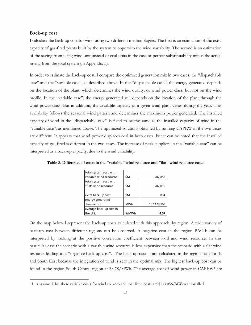
Back-up cost

I calculate the back-up cost for wind using two different methodologies. The first is an estimation of the extra

capacity of gas-fired plants built by the system to cope with the wind variability. The second is an estimation

of the saving from using wind unit instead of coal units in the case of perfect substitutability minus the actual

saving from the total system (in Appendix 3).

In order to estimate the back-up cost, I compare the optimized generation mix in two cases, the ―dispatchable

case‖ and the ―variable case‖, as described above. In the ―dispatchable case‖, the energy generated depends

on the location of the plant, which determines the wind quality, or wind power class, but not on the wind

profile. In the ―variable case‖, the energy generated still depends on the location of the plant through the

wind power class. But in addition, the available capacity of a given wind plant varies during the year. This

availability follows the seasonal wind pattern and determines the maximum power generated. The installed

capacity of wind in the ―dispatchable case‖ is fixed to be the same as the installed capacity of wind in the

―variable case‖, as mentioned above. The optimized solutions obtained by running CAPEW in the two cases

are different. It appears that wind power displaces coal in both cases, but it can be noted that the installed

capacity of gas-fired is different in the two cases. The increase of peak suppliers in the ―variable case‖ can be

interpreted as a back-up capacity, due to the wind variability.

Table 8. Difference of costs in the "variable" wind resource and "flat" wind resource cases

total system cost with

variable wind resource $M 202,853

total system cost with

"flat" wind resource $M 202,019

extra back-up cost $M 834

energy generated

from wind MWh 182,429,163

average back-up cost in

the U.S. $/MWh 4.57

On the map below I represent the back-up costs calculated with this approach, by region. A wide variety of

back-up cost between different regions can be observed. A negative cost in the region PACIF can be

interpreted by looking at the positive correlation coefficient between load and wind resource. In this

particular case the scenario with a variable wind resource is less expensive than the scenario with a flat wind

resource leading to a ―negative back-up cost‖. The back-up cost is not calculated in the regions of Florida

and South East because the integration of wind is zero in the optimal mix. The highest back-up cost can be

found in the region South Central region at $8.78/MWh. The average cost of wind power in CAPEW1 are

1 It is assumed that there variable costs for wind are zero and that fixed costs are $133 056/MW-year installed.

42

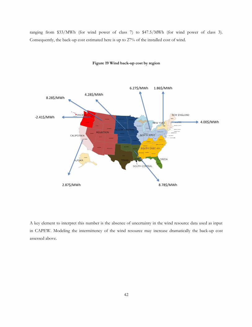
ranging from $33/MWh (for wind power of class 7) to $47.5/MWh (for wind power of class 3).

Consequently, the back-up cost estimated here is up to 27% of the installed cost of wind.

Figure 19 Wind back-up cost by region

8.28$/MWh4.28$/MWh

-2.41$/MWh

6.27$/MWh 1.86$/MWh

4.00$/MWh

8.78$/MWh2.87$/MWh

A key element to interpret this number is the absence of uncertainty in the wind resource data used as input

in CAPEW. Modeling the intermittency of the wind resource may increase dramatically the back-up cost

assessed above.

43

4.2 S3 “under projected fuel costs”

In the S3 scenario, ―under projected fuel costs‖, the fuel costs are $2.36/MMBtu for coal and $6.45/MMBtu

for gas. There is no carbon tax in this scenario S3. The penetration of wind power in the generation mix is

larger than in S1 ―under current fuel costs‖ because other technologies (coal-fired plants, IGCC with CCS,

NGCC and NGCC with CCS) have higher variable costs due to higher fuel costs. Wind power integration

varies widely across regions (from 0 to 55.6%). The total wind power installed capacity is 229GW1,

representing 22% of the total installed capacity in the U.S.

Figure 20. Installed capacity, S3 “under projected fuel costs”

0%

10%

20%

30%

40%

50%

60%

70%


inst

alle

d c

apac

ity

%

Generation mix S2 no carbon tax

pulverized_coal

NGCC

wind3

wind4

wind5

wind6

wind7

Figure 21. Integration of wind per region S3 “under projected fuel costs”

0.00%

10.00%

20.00%

30.00%

40.00%

50.00%

60.00%

70.00%

CA FL NY

NEN

GL

SEA

ST

NEA

ST

SCEN

T

NC

ENT TX

MO

UN

T

PA

CIF

% o

f in

stal

led

cap

acit

y

integration of wind S2 with no carbon tax


Table 9. Integration of wind per region, S2, no carbon tax



1 The current wind power installed capacity in the U.S. is around 40GW.

44

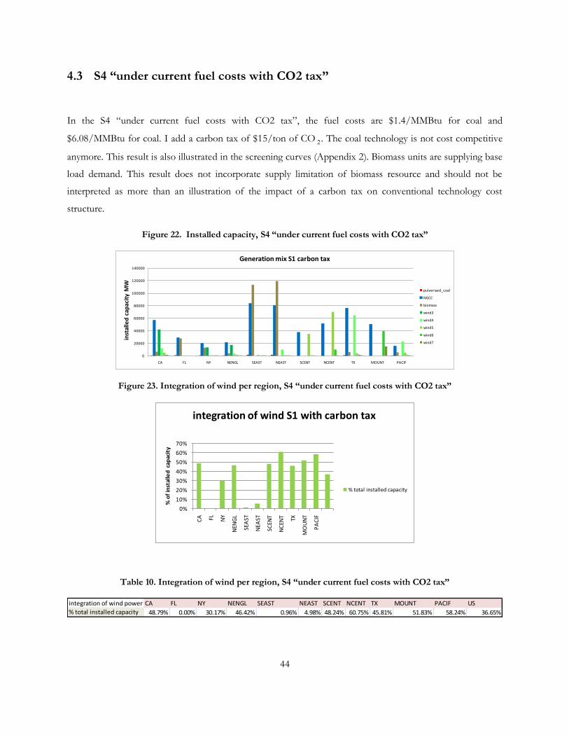
4.3 S4 “under current fuel costs with CO2 tax”

In the S4 ―under current fuel costs with CO2 tax‖, the fuel costs are $1.4/MMBtu for coal and

$6.08/MMBtu for coal. I add a carbon tax of $15/ton of CO 2 . The coal technology is not cost competitive

anymore. This result is also illustrated in the screening curves (Appendix 2). Biomass units are supplying base

load demand. This result does not incorporate supply limitation of biomass resource and should not be

interpreted as more than an illustration of the impact of a carbon tax on conventional technology cost

structure.

Figure 22. Installed capacity, S4 “under current fuel costs with CO2 tax”

0

20000

40000

60000

80000

100000

120000

140000


inst

alle

d c

apac

ity

MW

Generation mix S1 carbon tax

pulverized_coal

NGCC

biomass

wind3

wind4

wind5

wind6

wind7

Figure 23. Integration of wind per region, S4 “under current fuel costs with CO2 tax”

0%

10%

20%

30%

40%

50%

60%

70%

CA FL NY

NEN

GL

SEA

ST

NEA

ST

SCEN

T

NC

ENT TX

MO

UN

T

PA

CIF

% o

f in

stal

led

cap

acit

y

integration of wind S1 with carbon tax


Table 10. Integration of wind per region, S4 “under current fuel costs with CO2 tax”



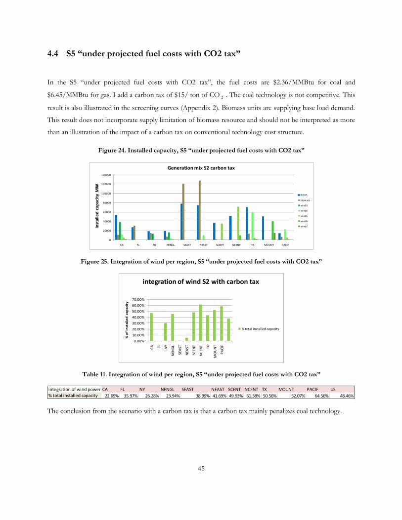
45

4.4 S5 “under projected fuel costs with CO2 tax”

In the S5 ―under projected fuel costs with CO2 tax‖, the fuel costs are $2.36/MMBtu for coal and

$6.45/MMBtu for gas. I add a carbon tax of $15/ ton of CO 2 . The coal technology is not competitive. This

result is also illustrated in the screening curves (Appendix 2). Biomass units are supplying base load demand.

This result does not incorporate supply limitation of biomass resource and should not be interpreted as more

than an illustration of the impact of a carbon tax on conventional technology cost structure.

Figure 24. Installed capacity, S5 “under projected fuel costs with CO2 tax”

0

20000

40000

60000

80000

100000

120000

140000


inst

alle

d c

apac

ity

MW

Generation mix S2 carbon tax

NGCC

biomass

wind3

wind4

wind5

wind6

wind7

Figure 25. Integration of wind per region, S5 “under projected fuel costs with CO2 tax”

0.00%

10.00%

20.00%

30.00%

40.00%

50.00%

60.00%

70.00%

CA FL NY

NEN

GL

SEA

ST

NEA

ST

SCEN

T

NC

ENT TX

MO

UN

T

PA

CIF

% o

f in

stal

led

cap

acit

y

integration of wind S2 with carbon tax


Table 11. Integration of wind per region, S5 “under projected fuel costs with CO2 tax”



The conclusion from the scenario with a carbon tax is that a carbon tax mainly penalizes coal technology.

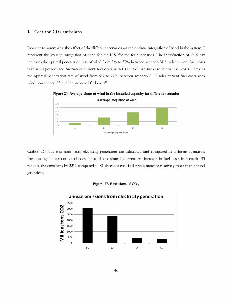
46

1. Cost and CO 2 emissions

In order to summarize the effect of the different scenarios on the optimal integration of wind in the system, I

represent the average integration of wind for the U.S. for the four scenarios. The introduction of CO2 tax

increases the optimal penetration rate of wind from 5% to 37% between scenario S1 ―under current fuel costs

with wind power‖ and S4 ―under current fuel costs with CO2 tax‖. An increase in coal fuel costs increases

the optimal penetration rate of wind from 5% to 22% between scenario S1 ―under current fuel costs with

wind power‖ and S3 ―under projected fuel costs‖.

Figure 26. Average share of wind in the installed capacity for different scenarios

0%

10%

20%

30%

40%

50%

60%

S1 S3 S4 S5

us average integration of wind

us average integration of wind

Carbon Dioxide emissions from electricity generation are calculated and compared in different scenarios.

Introducing the carbon tax divides the total emissions by seven. An increase in fuel costs in scenario S3

reduces the emissions by 22% compared to S1 (because coal fuel prices increase relatively more than natural

gas prices).

Figure 27. Emissions of CO 2

0

500

1000

1500

2000

2500

3000

3500

S1 S3 S4 S5

Mil

lion

s to

ns

CO

2

annual emissions from electricity generation

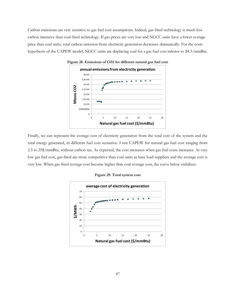
47

Carbon emissions are very sensitive to gas fuel cost assumptions. Indeed, gas-fired technology is much less

carbon intensive than coal-fired technology. If gas prices are very low and NGCC units have a lower average

price than coal units, total carbon emission from electricity generation decreases dramatically. For the costs

hypothesis of the CAPEW model, NGCC units are displacing coal for a gas fuel cost inferior to $4.3/mmBtu.

Figure 28. Emissions of CO2 for different natural gas fuel cost

0

500000000

1E+09

1.5E+09

2E+09

2.5E+09

3E+09

3.5E+09

4E+09

0 5 10 15 20 25 30

Mto

ns

CO

2

Natural gas fuel cost ($/mmBtu)

annual emissions from electricity generation

Finally, we can represent the average cost of electricity generation from the total cost of the system and the

total energy generated, in different fuel cost scenarios. I run CAPEW for natural gas fuel cost ranging from

2.5 to 25$/mmBtu, without carbon tax. As expected, the cost increases when gas fuel costs increases. At very

low gas fuel cost, gas-fired are more competitive than coal units as base load suppliers and the average cost is

very low. When gas-fired average cost become higher than coal average cost, the curve below stabilizes.

Figure 29. Total system cost

0

10

20

30

40

50

60

70

0 5 10 15 20 25 30

$/M

Wh

Natural gas fuel cost ($/mmBtu)

average cost of electricity generation

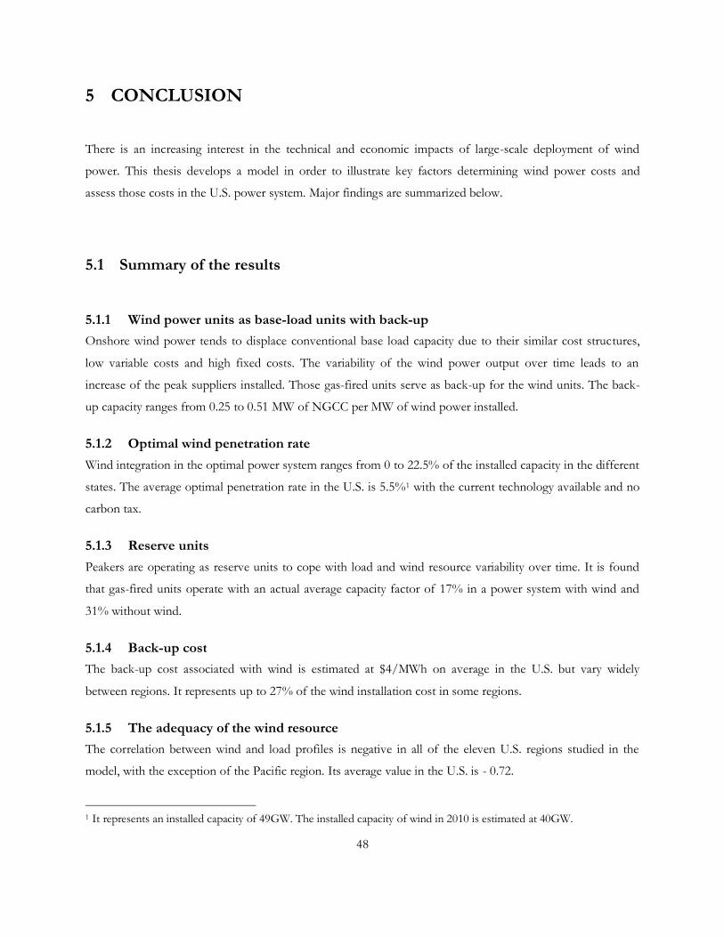
48

5 CONCLUSION

There is an increasing interest in the technical and economic impacts of large-scale deployment of wind

power. This thesis develops a model in order to illustrate key factors determining wind power costs and

assess those costs in the U.S. power system. Major findings are summarized below.

5.1 Summary of the results

5.1.1 Wind power units as base-load units with back-up

Onshore wind power tends to displace conventional base load capacity due to their similar cost structures,

low variable costs and high fixed costs. The variability of the wind power output over time leads to an

increase of the peak suppliers installed. Those gas-fired units serve as back-up for the wind units. The back-

up capacity ranges from 0.25 to 0.51 MW of NGCC per MW of wind power installed.

5.1.2 Optimal wind penetration rate

Wind integration in the optimal power system ranges from 0 to 22.5% of the installed capacity in the different

states. The average optimal penetration rate in the U.S. is 5.5%1 with the current technology available and no

carbon tax.

5.1.3 Reserve units

Peakers are operating as reserve units to cope with load and wind resource variability over time. It is found

that gas-fired units operate with an actual average capacity factor of 17% in a power system with wind and

31% without wind.

5.1.4 Back-up cost

The back-up cost associated with wind is estimated at $4/MWh on average in the U.S. but vary widely

between regions. It represents up to 27% of the wind installation cost in some regions.

5.1.5 The adequacy of the wind resource

The correlation between wind and load profiles is negative in all of the eleven U.S. regions studied in the

model, with the exception of the Pacific region. Its average value in the U.S. is - 0.72.

1 It represents an installed capacity of 49GW. The installed capacity of wind in 2010 is estimated at 40GW.

49

5.1.6 Introduction of a CO 2 tax

Introducing a carbon tax of $15/ton of CO 2 increases the optimal penetration rate of wind from 5% to 37%.

It also divides the total annual CO 2 emissions from electricity generation by 7 (from 3050 to 429 Mtons

CO 2/year). The total annual system cost increases by 17%.

5.2 Conclusions

It is found that wind power variability leads to an increase of the capacity installed of peak units and a

decrease in the actual capacity factor of those units. Therefore it is argued that dispatchable natural gas-fired

units serve as ―back-up‖. Peakers are operating as reserve units to cope with load and wind resource

variability over time. There is thus a back-up cost associated with wind varying widely across regions. The

optimal penetration rate of wind power in the U.S. varies with substantial variations across regions

A key factor influencing the optimal wind power integration rate is the correlation between wind resource and

load profiles, which are found to be negatively correlated in most U.S. regions. An increase in fossil fuel cost

leads to an increase in the optimal integration level of wind. Adding a carbon tax mainly penalizes coal

technology and increases the optimal integration level of wind power. Introducing a CO 2 tax increases the

optimal penetration rate of wind and increases the total annual system cost.

5.3 Limitations and Future work

An immediate extension of the present work is to include a representation of other renewable energy sources,

such as offshore wind, photovoltaic, solar thermal, geothermal, etc. The correlation between load and solar

resource may be positive. Indeed, solar irradiation is higher during midday and summer when the electricity

demand is high. The effect of introducing solar power may be an offset of wind variability.

A deterministic model was developed in the present thesis. Uncertainty is a critical issue for future

exploration. Indeed, modeling uncertainty is likely to increase the back-up cost and to reduce the optimal

penetration rate. Intermittency could be modeled by introducing a probabilistic representation of the wind

resource in the model.

50

One of the biggest challenges for the large-scale deployment of wind power in the U.S. is the extension of the

grid. Transmission is not modeled in the present thesis and could be added in future work. The transmission

cost of wind power integration in the system will be dependent of the distance between the wind resource

and the load.

To assess the economic and the environmental impacts of GHG mitigation policies, Computable General

Equilibrium (CGE) models are commonly used. This type of models captures effects between different

sectors of the economy. Prices and demand are endogenous in these models. However CGE models lack a

detailed representation of the electric sector. Indeed, in economy-wide models, or ‗top-down‘ models,

aggregated production functions poorly represent the different electric generation technologies. In particular

renewable energy technologies characteristics such as variability and intermittency are only partially

represented. One approach to capture the non-dispatchable nature of renewable is to consider an equivalent

technology of wind with back-up (Morris et. al. 2010). On the contrary, technology-rich engineering models,

‗bottom-up‘ models provide a detailed representation of electricity generating technologies and grid

transmission reliability issues. But these models are only partial equilibrium as they represent only the

electricity sector, or more broadly the energy sector. They typically lack the representation of interactions

among the various economic sectors. A future extension of the present work is to inform economic models

in the representation of renewables. Finally the optimal generation mix also depends on the amount of

storage capacity, interconnection and demand response in the power systems. All these components could be

added in the CAPEW model in future exploration.

A wide variety of climate policy tools have been designed to reduce GHGs emissions. One policy approach

tested by the CAPEW model is a carbon tax. The tax paid is equal to the marginal damages (Baumol 1972).

Taxing conventional electricity generation technologies can be justified by two main reasons; the need to

offset environmental externalities, and the need to create a competitive advantage to encourage the learning

process for new clean technologies. But designing and implementing this tool raises several issues, such as

political feasibility, timing, and complexity. As a tax would increase prices and might be difficult to agree on, a

second approach to maintain prices difference between carbon-intensive and clean technologies is to apply

lower tax on fossil-fuel technologies, or no tax, associated with a subsidy for renewable energy technologies.

Future work may include testing other policy tools, such as a Feed-in-Tariff or Renewable Portfolio Standard

(RPS).

Finally, most policy tools implemented are not taking into account the ―integration externality‖. The

unpredictable nature of renewables creates a negative externality associated with the integration of renewables

into the existing grid, due to costs of transmission lines extension, back-up units built, peakers units operated

51

as reserves, etc. They are thus likely to poorly evaluate wind power value in power systems. Consequently it is

suggested that a policy design including wind power capacity and back-up costs would improve future power

system planning.

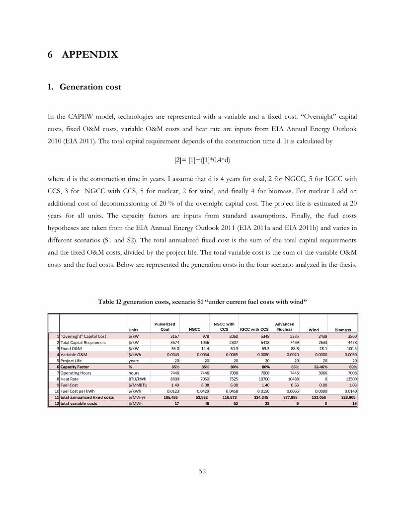
52

6 APPENDIX

1. Generation cost

In the CAPEW model, technologies are represented with a variable and a fixed cost. ―Overnight‖ capital

costs, fixed O&M costs, variable O&M costs and heat rate are inputs from EIA Annual Energy Outlook

2010 (EIA 2011). The total capital requirement depends of the construction time d. It is calculated by

[2]= [1]+([1]*0.4*d)

where d is the construction time in years. I assume that d is 4 years for coal, 2 for NGCC, 5 for IGCC with

CCS, 3 for NGCC with CCS, 5 for nuclear, 2 for wind, and finally 4 for biomass. For nuclear I add an

additional cost of decommissioning of 20 % of the overnight capital cost. The project life is estimated at 20

years for all units. The capacity factors are inputs from standard assumptions. Finally, the fuel costs

hypotheses are taken from the EIA Annual Energy Outlook 2011 (EIA 2011a and EIA 2011b) and varies in

different scenarios (S1 and S2). The total annualized fixed cost is the sum of the total capital requirements

and the fixed O&M costs, divided by the project life. The total variable cost is the sum of the variable O&M

costs and the fuel costs. Below are represented the generation costs in the four scenario analyzed in the thesis.

Table 12 generation costs, scenario S1 “under current fuel costs with wind”

Units

Pulverized

Coal NGCC

NGCC with

CCS IGCC with CCS

Advanced


1 "Overnight" Capital Cost $/kW 3167 978 2060 5348 5335 2438 3860

2 Total Capital Requirement $/kW 3674 1056 2307 6418 7469 2633 4478

3 Fixed O&M $/kW 36.0 14.4 30.3 69.3 88.8 28.1 100.5

4 Variable O&M $/kWh 0.0043 0.0034 0.0065 0.0080 0.0020 0.0000 0.0050

5 Project Life years 20 20 20 20 20 20 20

6 Capacity Factor % 85% 85% 80% 80% 85% 32-46% 80%

7 Operating Hours hours 7446 7446 7008 7008 7446 3066 7008

8 Heat Rate BTU/kWh 8800 7050 7525 10700 10488 0 13500

9 Fuel Cost $/MMBTU 1.40 6.08 6.08 1.40 0.63 0.00 1.03

10 Fuel Cost per kWh $/kWh 0.0123 0.0429 0.0458 0.0150 0.0066 0.0000 0.0140

11 total annualized fixed costs $/MW-yr 185,485 53,532 116,873 324,345 377,888 133,056 228,905

12 total variable costs $/MWh 17 46 52 23 9 0 19

53

Figure 30 generation costs, scenario S3 “under projected fuel costs”

Units

Pulverized

Coal NGCC

NGCC with

CCS IGCC with CCS

Advanced




Fixed O&M $/kW 36.0 14.4 30.3 69.3 88.8 28.1 100.5

Variable O&M $/kWh 0.0043 0.0034 0.0065 0.0080 0.0020 0.0000 0.0050


Capacity Factor % 85% 85% 80% 80% 85% 32-46% 80%


Heat Rate BTU/kWh 8800 7050 7525 10700 10488 0 13500

Fuel Cost $/MMBTU 2.36 6.45 6.45 2.36 0.63 0.00 1.03




Table 13 generation cost, scenario S4 “under current fuel costs with CO2 tax”

c_tax Units

Pulverized

Coal NGCC

NGCC with

CCS IGCC with CCS

Advanced




Fixed O&M $/kW 36.0 14.4 30.3 69.3 88.8 28.1 100.5

Variable O&M $/kWh 0.0043 0.0034 0.0065 0.0080 0.0020 0.0000 0.0050


Capacity Factor % 85% 85% 80% 80% 85% 32-46% 80%


Heat Rate BTU/kWh 8800 7050 7525 10700 10488 0 13500

Fuel Cost $/MMBTU 1.40 6.08 6.08 1.40 0.63 0.00 1.03


emissions g/kWh 800 300 200 700 60 0 60

tax $/MWh 0.012 0.0045 0.003 0.0105 0.0009 0 0.0009



Table 14 generation costs, scenario S5 “under projected fuel costs with CO2 tax”

c_tax Units

Pulverized

Coal NGCC

NGCC with

CCS IGCC with CCS

Advanced




Fixed O&M $/kW 36.0 14.4 30.3 69.3 88.8 28.1 100.5

Variable O&M $/kWh 0.0043 0.0034 0.0065 0.0080 0.0020 0.0000 0.0050


Capacity Factor % 85% 85% 80% 80% 85% 32-46% 80%


Heat Rate BTU/kWh 8800 7050 7525 10700 10488 0 13500

Fuel Cost $/MMBTU 2.36 6.45 6.45 2.36 0.63 0.00 1.03


emissions g/kWh 800 300 200 700 60 0 60

tax $/MWh 12 4.5 3 10.5 0.9 0 0.9



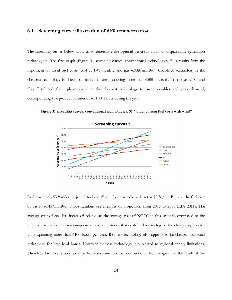
54

6.1 Screening curve illustration of different scenarios

The screening curves below allow us to determine the optimal generation mix of dispatchable generation

technologies. The first graph (Figure 31 screening curves, conventional technologies, S1 ) results from the

hypothesis of fossil fuel costs (coal at 1.4$/mmBtu and gas 6.08$/mmBtu). Coal-fired technology is the

cheapest technology for base-load units that are producing more than 4500 hours during the year. Natural

Gas Combined Cycle plants are then the cheapest technology to meet shoulder and peak demand,

corresponding to a production inferior to 4500 hours during the year.

Figure 31 screening curves, conventional technologies, S1 “under current fuel costs with wind”

-

10.00

20.00

30.00

40.00

50.00

60.00

70.00

0

30

0

60

0

90

0

1,2

00

1,5

00

1,8

00

2,1

00

2,4

00

2,7

00

3,0

00

3,3

00

3,6

00

3,9

00

4,2

00

4,5

00

4,8

00

5,1

00

5,4

00

5,7

00

6,0

00

6,3

00

6,6

00

6,9

00

7,2

00

7,5

00

7,8

00

8,1

00

8,4

00

8,7

00

Ave

rage

co

st (

$/M

Wh

)

hours

Screening curves S1

pulverized_coal

NGCC

NGCC_CCS

IGCC_CCS

nuclear

biomass

In the scenario S3 ―under projected fuel costs‖, the fuel cost of coal is set at $2.36/mmBtu and the fuel cost

of gas is $6.45/mmBtu. Those numbers are averages of projections from 2015 to 2035 (EIA 2011). The

average cost of coal has increased relative to the average cost of NGCC in this scenario compared to the

reference scenario. The screening curve below illustrates that coal-fired technology is the cheaper option for

units operating more than 6100 hours per year. Biomass technology also appears to be cheaper than coal

technology for base load hours. However biomass technology is subjected to regional supply limitations.

Therefore biomass is only an imperfect substitute to other conventional technologies and the result of the

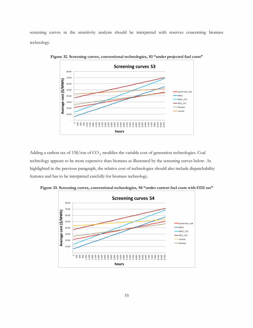
55

screening curves in the sensitivity analysis should be interpreted with reserves concerning biomass

technology.

Figure 32. Screening curves, conventional technologies, S3 “under projected fuel costs”

-

10.00

20.00

30.00

40.00

50.00

60.00

70.00

80.00

0

30

0

60

0

90

0

1,2

00

1,5

00

1,8

00

2,1

00

2,4

00

2,7

00

3,0

00

3,3

00

3,6

00

3,9

00

4,2

00

4,5

00

4,8

00

5,1

00

5,4

00

5,7

00

6,0

00

6,3

00

6,6

00

6,9

00

7,2

00

7,5

00

7,8

00

8,1

00

8,4

00

8,7

00

Ave

rage

co

st (

$/M

Wh

)

hours

Screening curves S3

pulverized_coal

NGCC

NGCC_CCS

IGCC_CCS

biomass

nuclear

Adding a carbon tax of 15$/ton of CO 2 modifies the variable cost of generation technologies. Coal

technology appears to be more expensive than biomass as illustrated by the screening curves below. As

highlighted in the previous paragraph, the relative cost of technologies should also include dispatchability

features and has to be interpreted carefully for biomass technology.

Figure 33. Screening curves, conventional technologies, S4 “under current fuel costs with CO2 tax”

-

10.00

20.00

30.00

40.00

50.00

60.00

70.00

80.00

0

30

0

60

0

90

0

1,2

00

1,5

00

1,8

00

2,1

00

2,4

00

2,7

00

3,0

00

3,3

00

3,6

00

3,9

00

4,2

00

4,5

00

4,8

00

5,1

00

5,4

00

5,7

00

6,0

00

6,3

00

6,6

00

6,9

00

7,2

00

7,5

00

7,8

00

8,1

00

8,4

00

8,7

00

Ave

rage

co

st (

$/M

Wh

)

hours

Screening curves S4

pulverized_coal

NGCC

NGCC_CCS

IGCC_CCS

nuclear

biomass

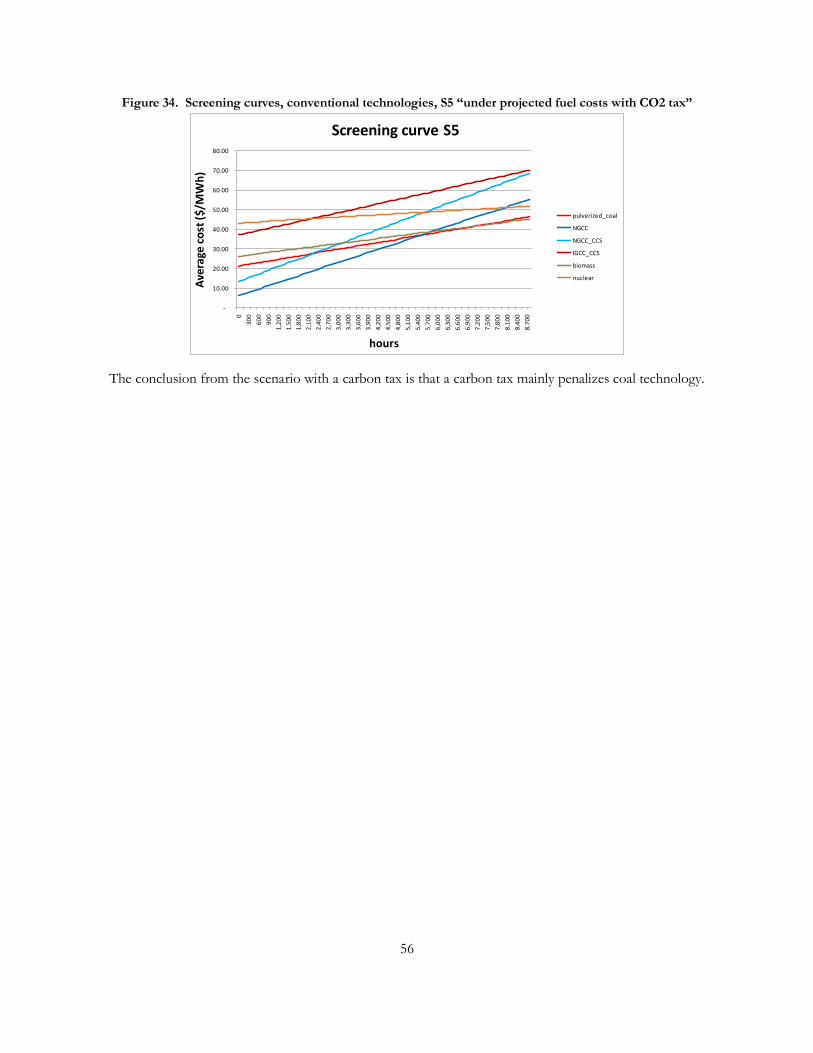
56

Figure 34. Screening curves, conventional technologies, S5 “under projected fuel costs with CO2 tax”

-

10.00

20.00

30.00

40.00

50.00

60.00

70.00

80.00

0

30

0

60

0

90

0

1,2

00

1,5

00

1,8

00

2,1

00

2,4

00

2,7

00

3,0

00

3,3

00

3,6

00

3,9

00

4,2

00

4,5

00

4,8

00

5,1

00

5,4

00

5,7

00

6,0

00

6,3

00

6,6

00

6,9

00

7,2

00

7,5

00

7,8

00

8,1

00

8,4

00

8,7

00

Ave

rage

co

st (

$/M

Wh

)

hours

Screening curve S5

pulverized_coal

NGCC

NGCC_CCS

IGCC_CCS

biomass

nuclear

The conclusion from the scenario with a carbon tax is that a carbon tax mainly penalizes coal technology.

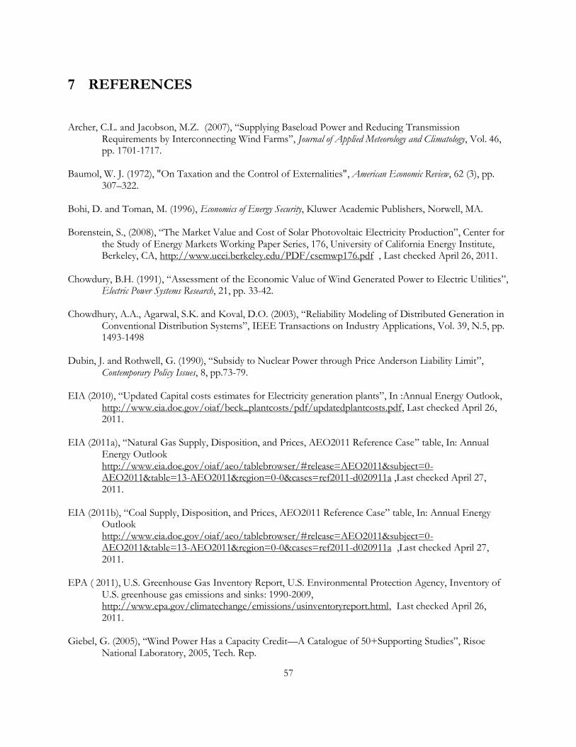
57

7 REFERENCES

Archer, C.L. and Jacobson, M.Z. (2007), ―Supplying Baseload Power and Reducing Transmission Requirements by Interconnecting Wind Farms‖, Journal of Applied Meteorology and Climatology, Vol. 46, pp. 1701-1717.

Baumol, W. J. (1972), "On Taxation and the Control of Externalities", American Economic Review, 62 (3), pp.

307–322. Bohi, D. and Toman, M. (1996), Economics of Energy Security, Kluwer Academic Publishers, Norwell, MA. Borenstein, S., (2008), ―The Market Value and Cost of Solar Photovoltaic Electricity Production‖, Center for

the Study of Energy Markets Working Paper Series, 176, University of California Energy Institute, Berkeley, CA, http://www.ucei.berkeley.edu/PDF/csemwp176.pdf , Last checked April 26, 2011.

Chowdury, B.H. (1991), ―Assessment of the Economic Value of Wind Generated Power to Electric Utilities‖,

Electric Power Systems Research, 21, pp. 33-42. Chowdhury, A.A., Agarwal, S.K. and Koval, D.O. (2003), ―Reliability Modeling of Distributed Generation in

Conventional Distribution Systems‖, IEEE Transactions on Industry Applications, Vol. 39, N.5, pp. 1493-1498

Dubin, J. and Rothwell, G. (1990), ―Subsidy to Nuclear Power through Price Anderson Liability Limit‖,

Contemporary Policy Issues, 8, pp.73-79. EIA (2010), ―Updated Capital costs estimates for Electricity generation plants‖, In :Annual Energy Outlook,

http://www.eia.doe.gov/oiaf/beck_plantcosts/pdf/updatedplantcosts.pdf, Last checked April 26, 2011.

EIA (2011a), ―Natural Gas Supply, Disposition, and Prices, AEO2011 Reference Case‖ table, In: Annual

Energy Outlook http://www.eia.doe.gov/oiaf/aeo/tablebrowser/#release=AEO2011&subject=0-AEO2011&table=13-AEO2011&region=0-0&cases=ref2011-d020911a ,Last checked April 27, 2011.

EIA (2011b), ―Coal Supply, Disposition, and Prices, AEO2011 Reference Case‖ table, In: Annual Energy

Outlook http://www.eia.doe.gov/oiaf/aeo/tablebrowser/#release=AEO2011&subject=0-AEO2011&table=13-AEO2011&region=0-0&cases=ref2011-d020911a ,Last checked April 27, 2011.

EPA ( 2011), U.S. Greenhouse Gas Inventory Report, U.S. Environmental Protection Agency, Inventory of

U.S. greenhouse gas emissions and sinks: 1990-2009, http://www.epa.gov/climatechange/emissions/usinventoryreport.html, Last checked April 26, 2011.

Giebel, G. (2005), ―Wind Power Has a Capacity Credit—A Catalogue of 50+Supporting Studies‖, Risoe

National Laboratory, 2005, Tech. Rep.

http://en.wikipedia.org/wiki/William_J._Baumol

http://www.jstor.org/stable/1803378

http://en.wikipedia.org/wiki/American_Economic_Review

http://www.ucei.berkeley.edu/PDF/csemwp176.pdf

http://www3.interscience.wiley.com/cgi-bin/fulltext/120001944/PDFSTART

http://www.eia.doe.gov/oiaf/beck_plantcosts/pdf/updatedplantcosts.pdf

http://www.eia.doe.gov/oiaf/aeo/tablebrowser/#release=AEO2011&subject=0-AEO2011&table=13-AEO2011&region=0-0&cases=ref2011-d020911a




http://www.epa.gov/climatechange/emissions/usinventoryreport.html

58

Gomez-Exposito, A., Conejo, J. and Canizares, C. (2009), Electric Energy Systems: Analysis and Operation, CRC

Press, New York, NY. Hobbs, B. F. (1995), ―Optimization Methods for Electric Utility Resource Planning‖, European Journal of

Operation Research, Vol. 83, pg 2. Holttinen, H., Milligan M., Kirby, B., Acker, T., Neimane, V. and Molinski, T. (2008), ―Using standard

deviation as a measure of increased operational reserve requirement for wind power‖, Wind Engineering, Vol. 32, No. 4., pp.355-378.

De Jonghe, C., Delarue, E., Belmans, R. and D'haeseleer, W. (2010), ―Determining optimal electricity

technology mix with high level of wind power penetration‖, Applied Energy, Vol. 88, Issue 6, pp. 2231-2238.

Joskow, P.L. (2010), ―Comparing the costs of intermittent and dispatchable electricit generating technologies‖

Report 2010-013, MIT Center for Energy and Environmental Policy Research, Cambridge, MA (USA), http://hdl.handle.net/1721.1/59468, Last checked April 26, 2011.

Kip,V.W., Harrington, J.E. and Vernon J.M. (1995) Economic of Regulation and Antitrust. The MIT Press,

Cambridge, MA. Kelly, H. and Weinberg, C.J. (1993), Utility strategies for using renewable, in Johansson,T.B., Kelly, H., Reddy,

A.K.N., Williams, R.H., (Eds), Renewable Energy: Sources for Fuels and Electricity, Island Press, Washington, DC.

Majumdar, S. and Chattopadhyay, D. (1999), ―A Model for Integrated Analysis of Generation Capacity

Expansion and Financial Planning‖, IEEE Transactions on Power Systems, Vol. 14 Issue 2, pg l. Malcom, S. A. and Zenios, S. A. (1994), ―Robust Optimization for Power Systems Capacity Expansion under

Uncertainty‖, The Journal of the Operational Research Society, Vol. 45, No. 9. Morris, J.F., Reilly, J.M. and Paltsev, S. (2010), ―Combining a Renewable Portfolio Standard with a Cap-and-

Trade Policy: a General Equilibrium Analysis‖, Report No. 187, MIT Joint Program of the Science and Policy of global change, Cambridge, MA (USA), http://globalchange.mit.edu/files/document/MITJPSPGC_Rpt187.pdf Last checked April 26, 2011.

Metcalf, G.E. (2007), "Federal Tax Policy Towards Energy." Tax Policy and the Economy, 21, 145-184 Milligan, M.R. (2000), ―Modeling Utility-Scale Wind Power Plants Part 2: Capacity Credit‖, Wind Energy, 3,

pp.167-206. Milligan, M.R. (1996), ―Measuring Wind Plant Capacity Value” WindStats Newsletter, Vol. 9, No. 1, Knebel,

Denmark. Moore, D.S.(1995), The Basic Practice of Statistics, Freeman, New York, NY. Nocedal, J. and Wright, S.J. (2006), Numerical Optimization, Second Edition, Springer, New York, NY.

http://www.sciencedirect.com/science/journal/03062619

http://www.sciencedirect.com/science?_ob=PublicationURL&_tockey=%23TOC%235683%232011%23999119993%232908780%23FLA%23&_cdi=5683&_pubType=J&view=c&_auth=y&_acct=C000022659&_version=1&_urlVersion=0&_userid=501045&md5=83162e37bc94da809fa39fa6b0339d9b

http://hdl.handle.net/1721.1/59468

http://www.jstor.org.libproxy.mit.edu/stable/i344544

http://globalchange.mit.edu/files/document/MITJPSPGC_Rpt187.pdf

59

Olson, M. (1971), The Logic of Collective Action: Public Goods and the Theory of Groups (Revised edition ed.). Harvard University Press, Cambridge, MA.

Parsons J.E. and Marcantonini C. (2010) ―Synthesis Report on Other Studies of the Levelised Cost of

electricity‖, In: Projected Costs of Generating Electricity http://www.oecd-nea.org/pub/egc/docs/exec-summary-ENG.pdf, Last checked April 26, 2011.

Palmintier, B. and Webster, M. (2011) ―Impact of Unit Commitment Constraints on Generation Expansion

Planning with Renewables‖, In Proceedings of 2011 IEEE Power and Energy Society General Meeting. To be presented at the 2011 IEEE Power and Energy Society General Meeting, Detroit, MI: IEEE.

Rausch, S., Metcalf, G.E., Reilly, J.M., and Paltsev, S. (2010), ―Distributional Implications of Alternative U.S.

Greenhouse Gas Control Measures,‖ The B.E. Journal of Economic Analysis & Policy, Vol. 10, Iss. 2. Shaalan, H.E. (2003), Generation of electric power, In: Beaty, H.W. (Ed.), Handbook of Electric Power Calculation, 3rd

ed., McGraw-Hill. Short, W., Blair, N., Heimiller, D. and Singhet V. (2003), ―Modeling the Long-Term Penetration of Wind in

the United States‖, National Renewable Energy Laboratory, CP-620-34469, Golden, CO. Short, W., Blair, N., Sullivan, P. and Mai, T. (2009), ―ReEDS Model Documentation: Base Case Data and

Model Description‖, National Renewable Energy Laboratory, Golden, CO, http://www.nrel.gov/analysis/reeds/pdfs/reeds_full_report.pdf , Last checked April 26, 2011.

Stigler, G.J. (1971), ―The Theory of Economic Regulation‖, Bell Journal of Economics and Management Science, 3,

pp. 3–18. United Nation (2008), ―World Population Prospects: The 2008 Revision‖, vol. I, Comprehensive Tables,

http://www.un.org/esa/population/publications/wpp2008/wpp2008_highlights.pdf, Last checked April 26, 2011.

Wan, Y. (2005), ―Primer on Wind Power for Utility Applications‖, National Renewable Energy Laboratory,

Report No. TP-50036230, Golden, CO. Wood, A.J. and Wollenberg, B.F. (1996), Power Generation, Operation, and Control, Second Edition, John Wiley &

Sons, Inc., New York, NY.

http://www.oecd-nea.org/pub/egc/docs/exec-summary-ENG.pdf

http://www.oecd-nea.org/pub/egc/docs/exec-summary-ENG.pdf

http://www.nrel.gov/analysis/reeds/pdfs/reeds_full_report.pdf

http://www.un.org/esa/population/publications/wpp2008/wpp2008_highlights.pdf

Documents

Economic and technical impacts of wind variability and ... 1.1 Motivation and context 1.1.1 Electricity, a commodity with unique features Electricity is an essential commodity with