Econometrica, Vol. 75, No. 1 (January, 2007), 83–119 Y EFFREY · 2013-02-05 · Econometrica, Vol. 75, No. 1 (January, 2007), 83–119 EXPERIMENTAL ANALYSIS OF NEIGHBORHOOD EFFECTS

Econometrica, Vol. 75, No. 1 (January, 2007), 83–119

EXPERIMENTAL ANALYSIS OF NEIGHBORHOOD EFFECTS

BY JEFFREY R. KLING, JEFFREY B. LIEBMAN, AND LAWRENCE F. KATZ1

Families, primarily female-headed minority households with children, living in high-poverty public housing projects in five U.S. cities were offered housing vouchers bylottery in the Moving to Opportunity program. Four to seven years after random as-signment, families offered vouchers lived in safer neighborhoods that had lower povertyrates than those of the control group not offered vouchers. We find no significant over-all effects of this intervention on adult economic self-sufficiency or physical health.Mental health benefits of the voucher offers for adults and for female youth were sub-stantial. Beneficial effects for female youth on education, risky behavior, and physicalhealth were offset by adverse effects for male youth. For outcomes that exhibit sig-nificant treatment effects, we find, using variation in treatment intensity across vouchertypes and cities, that the relationship between neighborhood poverty rate and outcomesis approximately linear.

KEYWORDS: Social experiment, housing vouchers, neighborhoods, mental health,urban poverty.

THE RESIDENTS OF DISADVANTAGED NEIGHBORHOODS fare substantiallyworse on a wide range of socioeconomic and health outcomes than dothose with more affluent neighbors. Economic models of residential sorting—partially motivated by these observed associations between neighborhoodcharacteristics and individual outcomes—suggest that inefficient equilibria canarise when individual outcomes are influenced by neighbors and individuals donot take their external effects on neighbors into account in their location deci-sions (e.g., Benabou (1993)).

1This paper integrates material previously circulated in Kling and Liebman (2004), Kling,Liebman, Katz, and Sanbonmatsu (2004), and Liebman, Katz, and Kling (2004). Support forthis research was provided by grants from the U.S. Department of Housing and Urban Devel-opment (HUD), the National Institute of Child Health and Development (NICHD), and theNational Institute of Mental Health (R01-HD40404 and R01-HD40444), the National ScienceFoundation (9876337 and 0091854), the Robert Wood Johnson Foundation, the Russell SageFoundation, the Smith Richardson Foundation, the MacArthur Foundation, the W. T. GrantFoundation, and the Spencer Foundation. Additional support was provided by grants to PrincetonUniversity from the Robert Wood Johnson Foundation and from NICHD (5P30-HD32030 for theOffice of Population Research), by the Princeton Industrial Relations Section, the Bendheim–Thomas Center for Research on Child Wellbeing, the Princeton Center for Health and Wellbe-ing, and the National Bureau of Economic Research. We are grateful to Todd Richardson andMark Shroder of HUD; to Eric Beecroft, Judie Feins, Barbara Goodson, Robin Jacob, StephenKennedy, Larry Orr, and Rhiannon Patterson of Abt Associates; to our collaborators JeanneBrooks-Gunn, Alessandra Del Conte Dickovick, Greg Duncan, Tama Leventhal, Jens Ludwig,Bruce Psaty, Lisa Sanbonmatsu, and Robert Whitaker; to our research assistants Ken Fortson,Jane Garrison, Erin Metcalf, and Josh Meltzer; and to numerous colleagues and three anony-mous referees for valuable suggestions. Any findings or conclusions expressed are those of theauthors.

83

http://www.econometricsociety.org/

84 J. R. KLING, J. B. LIEBMAN, AND L. F. KATZ

It is hard to judge from theory alone whether the externalities from havingneighbors of higher socioeconomic status are predominantly beneficial (fromsocial connections, positive role models, reduced exposure to violence, andmore community resources), inconsequential (only family influences, geneticendowments, individual human capital investments, and the broader nonneigh-borhood social environment matter), or adverse (from competition with ad-vantaged peers and discrimination).2 Empirical assessment of the importanceof such externalities has also proven difficult using nonexperimental data be-cause individuals sort across neighborhoods for reasons that are likely to becorrelated with the underlying determinants of their outcomes.

In this paper, we avoid the problem of endogenous neighborhood selectionby using data from a randomized experiment in which some families living inhigh-poverty U.S. housing projects were offered Section 8 housing vouchersto enable them to move to lower poverty neighborhoods while others werenot offered vouchers.3 Thus our analysis provides direct evidence on the ex-istence, direction, and magnitude of neighborhood effects for important so-cioeconomic and health outcomes in both adult and youth populations. Thefindings also bear on key housing policy decisions such as whether it is betterto provide housing subsidies tied to public housing projects or housing vouch-ers that can be used in the private-sector rental market.

The research design used in this paper is based on comparisons of threegroups to which households were randomly assigned in the Moving to Oppor-tunity (MTO) social experiment operated in five cities—Baltimore, Boston,Chicago, Los Angeles, and New York—by the U.S. Department of Housingand Urban Development. A control group received no new assistance, butcontinued to be eligible for public housing. A Section 8 group received a tra-ditional Section 8 voucher, without geographic restriction. An experimentalgroup received a Section 8 voucher restricted for 1 year to a census tract with apoverty rate of less than 10 percent and also received mobility counseling. Oursample consists of 4,248 households assigned from 1994–1997 at the five sites.

In 2002, extensive data were collected on outcomes from five key domains:economic self-sufficiency, mental health, physical health, risky behavior, andeducation. This paper provides the main results from MTO for adults and foryouth ages 15–20 at all five sites an average of 5 years after random assignment,

2See, for example, Jencks and Mayer (1990), Becker and Murphy (2000), Brock and Durlauf(2001), and Kawachi and Berkman (2003).

3Low-income U.S. families receive federal housing assistance through subsidies tied to resi-dence in public housing projects or through vouchers (now called Housing Choice Vouchers, butcommonly known as Section 8) that subsidize rents for private sector units. These programs arenot entitlements and have wait lists that can be substantial. Tenants in U.S. public housing andthose whose use Section 8 housing vouchers both pay approximately 30 percent of their incomesin rent. The value of a voucher is the difference between 30 percent of income and the city’s fairmarket rent, set at the 40th percentile of area rents. See Olsen (2003) for an overview of U.S.housing programs for the poor.

NEIGHBORHOOD EFFECTS 85

providing the most comprehensive experimental analysis to date of neighbor-hood effects.4

1. DATA AND DESCRIPTIVE STATISTICS

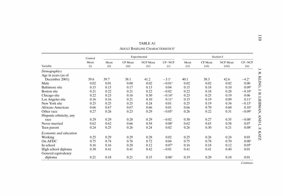
The data for this study come from a baseline survey, administrative data,and an impact evaluation survey conducted in 2002 of one adult and up to tworandomly selected children in each MTO household. The baseline survey wasadministered to household heads prior to random assignment. Administrativedata on earnings and welfare benefits were obtained from state and countyagencies in California, Illinois, Maryland, Massachusetts, and New York.5 The2002 survey had an effective response rate of 90 percent for adults and femaleyouth and 86 percent for male youth.6 All statistical estimates in this paperuse weights.7 The baseline covariates included in our reported regressions aredisplayed in Appendix A, Tables A1 and A2 for adults and youth, respectively.Details of the outcome variables are provided in Appendix A.

The Boston, Los Angeles, and New York families in our sample are mainlyblack or Hispanic; those in Baltimore and Chicago are nearly all black. Overall,

4Additional results are available from Sanbonmatsu, Kling, Duncan, and Brooks-Gunn (2006),who analyzed reading and math test scores for children ages 6–20, and from Kling, Ludwig, andKatz (2005), who analyzed arrest records for youth ages 15–25. The earlier single-site pilot studiesof MTO are collected in Goering and Feins (2003). Detailed background information on theMTO demonstration and the interim evaluation survey is contained in Orr et al. (2003).

5Four states provided individual-level earnings information on each MTO sample memberwho matched to the Unemployment Insurance (UI) records. Massachusetts provided only dataaggregated to groups that consisted of at least 10 MTO individuals. Agency data were linkedby Social Security number using information only from the state in which the sample memberresided at the time of random assignment. Earnings and welfare amounts were inflation adjustedto 2001 dollars using the Consumer Price Index for all urban consumers.

6An initial phase from January–June 2002 resulted in an 80% response rate for adults. At thatpoint, we drew a 3-in-10 subsample of remaining cases and located 48% of them. The purpose ofthe subsampling was to concentrate resources on finding hard-to-locate families so as to minimizethe potential for nonresponse bias. We calculate the effective response rate for adults as 80+(1−0�8)× 48 = 89�6. The effective response rate for youths is calculated using this same approach.

7The weights have three components (Orr et al. (2003)). First, subsample members receivegreater weight because, in addition to themselves, they represent individuals who we did not at-tempt to contact during the subsampling phase. Second, youth from large families receive greaterweight because we randomly sampled two children per household, implying that youth from largefamilies are representative of a larger fraction of the study population; this component does notapply to adults. Third, all individuals are weighted by the inverse of their probability of assignmentto their experimental group to account for changes in the random assignment ratios over time.The ratio of individuals randomly assigned to treatment groups was changed during the courseof the demonstration to minimize the minimum detectable effects after take-up of the vouchersturned out to be different than had been projected. This third component of the weights preventstime or cohort effects from confounding the results. Our weights imply that each random assign-ment period is weighted in proportion to the number of people randomly assigned in that period.Analyses of administrative data use only the third component of the weights.


85 percent of the households are female-headed and either African–Americanor Hispanic. Ninety-eight percent of the sample adults are female, and 93 per-cent were ages 25–54 as of December 31, 2001. At the time of random as-signment, one quarter of sample adults were employed, three-quarters werereceiving Aid for Families with Dependent Children (AFDC), more than halfhad never married, fewer than half had graduated from high school, and aquarter had been teenage parents. In a baseline survey, a majority said theywanted to move out of public housing “to get away from drugs and gangs.”

Participants volunteered for this study, presumably because they were inter-ested in moving out of their original high-poverty neighborhoods. Althoughthis may be the most relevant population when considering incremental ex-pansion of the use of housing vouchers to replace public housing, care shouldbe taken in applying these results to populations with different characteristics.The experiment did not result in large clusters of moves to the same new neigh-borhoods; therefore, it is unlikely to have had large effects on receiving neigh-borhoods or via “social multiplier” or “general equilibrium” effects (Manski(1993), Heckman (2001)).

Families in the treatment groups had 4–6 months to find qualified housingand move using a MTO voucher. The fraction of treatment group familieswho used a MTO voucher to move, which we refer to as the compliance rate,was 47 percent for the experimental group and 60 percent for the Section 8group. Compared to noncompliers (those in the treatment groups who did notuse a MTO voucher), compliers (those who moved using a MTO voucher)were younger and more likely to have had no teenage children at baseline, tohave reported that their neighborhood was very unsafe at night, to have saidthat they were very dissatisfied with their apartment, to have been enrolled inschool, and to have forecast that they would be “very likely” to find a new apart-ment if offered a voucher. Compliance rates differed substantially by site froma low of 32 percent in the Chicago experimental group to a high of 77 percentin the Los Angeles Section 8 group.8

To characterize the neighborhoods in which families lived and the differ-ences in residential location for those who used a MTO voucher versus thosewho did not, Figure 1 shows several densities of neighborhood (census tract)poverty rates. The poverty rates are duration-weighted averages over locationslived at since random assignment and they use linear interpolation for povertyrates between the Census years of 1990 and 2000. Figure 1 indicates that exper-imental compliers lived in neighborhoods with significantly lower poverty ratesthan did controls, with nearly 60 percent living in neighborhoods below 20 per-cent poverty; Section 8 compliers also lived in lower poverty neighborhoods,

8The intensity of housing search assistance provided to the experimental group by the non-profits responsible for the counseling varied considerably across sites, as did the tightness of localhousing markets.


FIGURE 1.—Densities of average poverty rate, by group. Average poverty rate is a dura-tion-weighted average of tract locations from random assignment through 12/31/2001. Povertyrate is based on linear interpolation of 1990 and 2000 Censuses. Density estimates used anEpanechnikov kernel with a half-width of 2.

but their density is shifted by a more modest amount. The densities for exper-imental noncompliers, Section 8 noncompliers, and controls are quite similarto each other.9

Additional descriptive statistics of the residential locations are shown in Ta-ble I. The experimental and Section 8 groups are both substantially less likelyto live in very poor areas with visible drug activity, and somewhat more likely tolive in areas with greater adult employment and a lower share of minority resi-dents. Members of the treatment groups feel safer and are less likely to report ahousehold member having been victimized by crime in the previous 6 months.The 0.82 average share minority for experimental group tracts indicates thatalthough families moved to lower poverty census tracts, these families did notmove to distant white suburban areas. In the experimental group, only 16 per-cent moved 10 miles or more, and only 12 percent had an average tract shareminority less than half (Appendix, Table F2 in the supplement to this article(Kling, Liebman, and Katz (2007)), hereafter referenced as Web Appendix).

9This implies that there was little selection of the type typically hypothesized, where complierswould have been more likely to have moved to lower poverty neighborhoods even if they had notbeen offered a voucher (and the poverty distribution for controls would therefore exhibit greaterdensity at lower neighborhood-poverty rates than would the density for noncompliers).

88J.R

.KL

ING

,J.B.L

IEB

MA

N,A

ND

L.F.K

AT

Z

TABLE I

DESCRIPTIVE STATISTICS OF NEIGHBORHOOD CHARACTERISTICSa

Experimental Section 8 Control(i) (ii) (iii)

Average census tract poverty rate 0.33 0.35 0.45Average census tract poverty rate above 30% 0.52 0.62 0.87Respondent saw illicit drugs being sold or used in neighborhood during past 30 days 0.33 0.34 0.46Streets are safe or very safe at night 0.70 0.65 0.56Member of household victimized by crime during past 6 months 0.17 0.16 0.21Average census tract share on public assistance 0.16 0.17 0.23Average census tract share of adults employed 0.83 0.83 0.78Average census tract share workers in professional and managerial occupations 0.26 0.23 0.21Average census tract share minority 0.82 0.87 0.90

aCensus tract characteristics are the average for an individual’s addresses from randomization through 2001 weighted by duration. Except for “professional and managerialoccupations” (for which only 2000 Census data were used due to differences in the occupation classification used for the 1990 Census and 2000 Census), values for intercensusyears are interpolated. “Saw illicit drugs,” “streets are safe,” and “victimized by crime” are based on adult report in the 2002 survey. All experimental − control and Section 8 −control differences have p-values < 0�05.


2. ANALYSIS

We focus on 15 primary outcomes for adults and 15 primary outcomes foryouth. Prior to examining the data, we decided to examine youth results pooledby gender and separately for females and males—both because the prevalencefor some outcomes differs greatly by gender and results in different statisticalpower to detect effects and because there had been some evidence of morebeneficial effects for boys in earlier MTO research (Katz, Kling, and Liebman(2001), Ludwig, Duncan, and Hirschfield (2001)) and in welfare reform re-search (Bos et al. (1999)). With 15 outcomes, four population groups (adults,all youth, female youth, and male youth), and two treatment groups, there is atotal of 120 treatment effect estimates in this set.

To draw general conclusions about the experiment’s results, we first presentfindings for summary indices that aggregate information over multiple treat-ment effect estimates (later we present estimates for specific outcomes). Forexample, we create an index of economic self-sufficiency that averages togetherfive measures of employment, earnings, and public assistance receipt. The ag-gregation improves statistical power to detect effects that go in the same di-rection within a domain.10 The summary index Y is defined to be the equallyweighted average of z-scores of its components, with the sign of each mea-sure oriented (as indicated in the notes to Table II) so that more beneficialoutcomes have higher scores. The z-scores are calculated by subtracting thecontrol group mean and dividing by the control group standard deviation.11

Thus, each component of the index has mean 0 and standard deviation 1 forthe control group.

We begin by estimating intent-to-treat (ITT) effects—differences betweentreatment and control group means. Estimation of the ITT effect π1 is fromEquation (1). Let Z be an indicator for treatment group assignment and letX be a matrix of baseline covariates:

Y = Zπ1 +Xβ1 + ε1�(1)

10O’Brien (1984) constructed a global test statistic for multiple outcomes with maximum poweragainst the alternative that all effects have the same sign and effect size. An adaptation of theO’Brien approach is discussed in Appendix B of the Web Appendix and implemented in Klingand Liebman (2004), which uses seemingly unrelated regression effects for specific outcomes toestimate the covariance of the effects and calculates the mean effect size for groups of estimatesin a second step. The average z-score index used in this paper is much simpler to work with, par-ticularly for our results that relate neighborhood poverty rates to outcomes. The two approachesyield identical treatment effects when there is no item nonresponse and no regression adjustment.

11If an individual has a valid response to at least one component measure of an index, thenany missing values for other component measures are imputed at the random assignment groupmean. This results in differences between treatment and control means of an index being thesame as the average of treatment and control means of the components of that index (when thecomponents are divided by their control group standard deviation and have no missing valueimputation), so that the index can be interpreted as the average of results for separate measuresscaled to standard deviation units.

90J.R

.KL

ING

,J.B.L

IEB

MA

N,A

ND

L.F.K

AT

Z

TABLE II

MEAN EFFECT SIZES FOR SUMMARY MEASURES OF OUTCOMESa

All Adults All Youth Female Youth Male Youth M−F Youth

E−C S−C E−C S−C E−C S−C E−C S−C E−C S−C(i) (ii) (iii) (iv) (v) (vi) (vii) (viii) (ix) (x)

Economic 0.017 0.037self-sufficiency (0.031) (0.033)

Absence of physical 0.012 0.019 −0.038 −0.020 0.025 0.077 −0.112∗ −0.114 −0.138 −0.192∗

health problems (0.024) (0.026) (0.038) (0.040) (0.053) (0.055) (0.053) (0.061) (0.076) (0.084)Absence of mental 0.079∗ 0.029 0.102 0.138∗ 0.267∗ 0.192∗ −0.052 0.054 −0.319∗ −0.138

health problems (0.030) (0.033) (0.053) (0.056) (0.062) (0.067) (0.080) (0.092) (0.101) (0.113)Absence of risky −0.023 −0.039 0.142∗ 0.129∗ −0.181∗ −0.208∗ −0.323∗ −0.337∗

behavior (0.043) (0.050) (0.053) (0.059) (0.062) (0.071) (0.080) (0.092)Education 0.050 0.028 0.138∗ 0.056 −0.053 −0.001 −0.191∗ −0.057

(0.041) (0.047) (0.065) (0.068) (0.047) (0.060) (0.080) (0.090)Overall 0.036 0.028 0.018 0.018 0.136∗ 0.109∗ −0.099∗ −0.078∗ −0.235∗ −0.187∗

(0.020) (0.022) (0.025) (0.026) (0.034) (0.034) (0.031) (0.037) (0.047) (0.051)aE − C denotes experimental − control; S − C denotes Section 8 − control. Estimates are the intent-to-treat mean effect sizes, from Equation (1), fully interacted with gender

in columns (v)–(x) as described in the text. The estimated equations all include site indicators and the baseline covariates listed in Appendix A with those in Table A1 included foradults and those in Tables A1 and A2 included for youth. M − F Youth is male − female difference. Adult economic self-sufficiency: + adult not employed and not on TANF +employed + 2001 earnings − on TANF − 2001 government income. Adult mental health: − distress index − depression symptoms − worrying + calmness + sleep. Adult physicalhealth: − self-reported health fair/poor − asthma attack past year − obesity − hypertension − trouble carrying/climbing. Adult overall includes 15 measures in self-sufficiency,physical health, and mental health. Youth physical health: − self-reported health fair/poor − asthma attack past year − obesity − nonsports injury past year. Youth mental health:− distress index − depression symptoms − anxiety symptoms. Youth risky behavior: − marijuana past 30 days − smoking past 30 days − alcohol past 30 days − ever pregnantor gotten someone pregnant. Youth education: + graduated high school or still in school + in school or working + WJ-R broad reading score + WJ-R broad math score. Youthoverall includes 15 measures in physical health, mental health, risky behavior, and education. Sample sizes in the E, S, and C groups are 1,453, 993, and 1,080 for adults and 749,510, and 548 for youth ages 15–20 on 12/31/2001. Robust standard errors adjusted for household clustering are in parentheses; * = p-value < 0.05.


The covariates (X) are included to improve estimation precision and to ac-count for chance differences between groups in the distribution of pre-random-assignment characteristics. Table II shows ITT results by domain and popula-tion group for indices, with the measures included in each index indicated inthe notes to Table II and the details on each measure presented in AppendixA. The absolute magnitudes of the indices are in units akin to standardizedtest scores: the ITT estimate shows where the mean of the treatment group isin the distribution of the control group in terms of standard deviation units.

For adults, the direction of effects is positive for both the experimental andSection 8 groups relative to the control group for all three domains: economicself-sufficiency, physical health, and mental health. The effect on mental healthfor the experimental group is much larger in magnitude than the others and isthe only adult estimate that is statistically significant at the 5 percent level. Forresults that pool all youth, the direction of effects is positive for mental healthand education, and negative for physical health and risky behavior. Again,the effects on mental health (for both the experimental group and Section 8groups) are much larger and have p-values below 0.06. For the overall indexthat averages together all fifteen outcomes, the results in columns (i)–(iv) foradults and for all youth are positive in sign, but the magnitudes are not largeenough to reject a null hypothesis of no effect with 95 percent confidence.Thus, for adults and for all youth, the evidence of effects from relocation tolower poverty neighborhoods is strongest for the domain of mental health.

The overall results for youth average together estimates that differ substan-tially for female and male youth. Columns (v)–(viii) of Table II show large pos-itive effects on mental health and risky behavior for female youth, and largenegative effects on physical health and risky behavior for male youth.12 Thisgender pattern in results was the opposite of what we expected.13 Yet, as shownin columns (ix) and (x), the medium-term effects for females are more benefi-cial than for males for all four domains and in both treatment groups relativeto the control group.

As a complement to the summary indices, we also examined results for eachspecific outcome that was a component of an index. Because the magnitudesof these separate outcomes are often easier to interpret than those of the sum-mary indices, we show in Table III all outcomes with ITT effects significantat the 5 percent level. In addition to ITT effects, we also report the effect oftreatment-on-treated (TOT) for these measures. We estimate this effect using

12These results are based on estimation of Y = (1 −G)(Xβ10 +Zπ10)+G(Xβ11 +Zπ11)+υ,where G is an indicator for gender, and X includes household and individual-specific character-istics.

13Existing nonexperimental papers find larger beneficial effects for boys from living in advan-taged neighborhoods than for girls (examples include Entwisle, Alexander, and Olson (1994),Ramirez-Valles, Zimmerman, and Juarez (2002), and Crane (1991)). The predominant mecha-nism proposed in these studies is that boys spend more time hanging out in the neighborhoodand, therefore, are influenced more heavily by the neighborhood.


TABLE III

SPECIFIC OUTCOMES WITH EFFECTS SIGNIFICANT AT 5 PERCENT LEVELa

E/S CM ITT TOT CCM(i) (ii) (iii) (iv) (v)

A. Adult outcomesObese, BMI≥ 30 E−C 0.468 −0.048 −0.103 0.502

(0.022) (0.047)Calm and peaceful E−C 0.466 0.061 0.131 0.443

(0.022) (0.047)Psychological distress, K6 z-score E−C 0.050 −0.092 −0.196 0.150

(0.046) (0.099)

B. Youth (female and male) outcomesEver had generalized anxiety symptoms E −C 0.089 −0.044 −0.099 0.164

(0.019) (0.042)S−C 0.089 −0.063 −0.114 0.147

(0.019) (0.035)Ever had depression symptoms S−C 0.121 −0.039 −0.069 0.134

(0.019) (0.035)

C. Female youth outcomesPsychological distress, K6 scale z-score E−C 0.268 −0.289 −0.586 0.634

(0.094) (0.197)Ever had generalized anxiety symptoms E−C 0.121 −0.069 −0.138 0.207

(0.027) (0.055)S−C 0.121 −0.075 −0.131 0.168

(0.029) (0.051)Used marijuana in the past 30 days E−C 0.131 −0.065 −0.130 0.202

(0.029) (0.059)S−C 0.131 −0.072 −0.124 0.209

(0.032) (0.056)Used alcohol in past 30 days S−C 0.206 −0.091 −0.155 0.306

(0.038) (0.056)

D. Male youth outcomesSerious nonsports accident or injury E−C 0.062 0.087 0.215 0in past year (0.026) (0.064)

S−C 0.062 0.080 0.157 0(0.028) (0.058)

Ever had generalized anxiety symptoms S−C 0.055 −0.049 −0.098 0.126(0.024) (0.047)

Smoked in past 30 days E−C 0.125 0.103 0.257 0(0.032) (0.084)

S−C 0.125 0.151 0.293 0.014(0.037) (0.073)

aE/S: indicates whether the row is experimental − control (E − C) or Section 8 − control (S − C). CM, controlmean; ITT, intent-to-treat, from Equation (1); TOT, treatment-on-treated, from Equation (2); CCM, control com-plier mean. Robust standard errors adjusted for household clustering are in parentheses. The estimated equations allinclude site indicators and the baseline covariates listed in Appendix A with those in Table A1 included for adults andthose in Tables A1 and A2 for youth. Rows shown in the table to illustrate magnitudes were selected based on ITTp-values < 0.05 and are 17 of 120 from the set of specific contrasts (E − C, S − C), based on the outcomes (15 foradults and 15 for youth) and subgroups—adults, youth (female and male), female youth, and male youth—describedin the notes to Table II.


the offer of a MTO voucher as an instrumental variable for MTO voucher use,so Z is the excluded instrument for an indicator D of compliance in the twostage least squares (2SLS) estimation:

Y = Dγ2 +Xβ2 + ε2�(2)

The TOT parameter γ2 is equal to the ITT parameter divided by theregression-adjusted compliance rate. We interpret these 2SLS estimates astreatment-on-treated estimates rather than local average treatment effect esti-mates (Imbens and Angrist (1994)) because the endogenous variable is use ofa voucher offered by the MTO program, and MTO vouchers are never offeredto the control group; there are no always-takers in the terminology of Angrist,Imbens, and Rubin (1996).14 This TOT approach relies on the assumption thatthere was no average effect of being offered a MTO voucher on those whodid not use a MTO voucher, which we believe is a reasonable approximation,but not strictly true.15 Under this assumption, we can assess the average mag-nitude of the effect of the voucher offer for those who complied and used aMTO voucher to move to a lower poverty neighborhood.

As an example, results for the outcome of adult obesity, using a standardbody mass index cut point (BMI ≥ 30 kg/m2), are shown in the first row ofTable III. The results in column (i) indicate that this row compares the experi-mental and control groups (E − C). Column (iii) reveals that the ITT effect onobesity is a 5 percentage point reduction in obesity for the experimental grouprelative to the control group. Assuming no effect on those who did not use aMTO voucher to move, the TOT effect was just over 10 percentage points.

Because outcomes are directly observed for treatment group compliers andwe have a TOT estimate, we can estimate the mean level of each outcome forthose in the control group who would have complied if they had been offered avoucher—which we refer to as the control complier mean (CCM; Katz, Kling,and Liebman (2001))—based on the relationship that CCM = E[Y |Z = 1�

14See, also, Heckman (1990). Over time, some control group members do receive housingvouchers from other sources, but they tend to receive them significantly later than treatmentgroup members do. Therefore, in our TOT estimates, we do not define control group voucherrecipients as having been treated. We do interpret both our ITT and TOT estimates as averagesof heterogeneous treatment effects across individuals.

15For the experimental group, this assumption implies that the later outcomes of householdswho met with a housing mobility counselor were not affected by the counselor if that householddid not make a subsidized move through the MTO program. For both treatment groups, thisassumption implies that the experience of housing search induced by assignment to a treatmentgroup did not affect later outcomes if that household did not make a subsidized program move.For noncompliers, we believe that the effects of mobility counselors (who mainly provided hous-ing advice and not general social services) on self-sufficiency and health outcomes are likely to beorders of magnitude smaller than the effects of moving to a new residential location. The TOTapproach also requires that the control group was not affected by the experience of losing thevoucher lottery, something we view as a reasonable approximation.


D= 1] −γ.16 For the fraction obese, the CCM in column (v) is estimated to be0.502.17 Thus a 10 percentage point change would be a decline in relative riskamong compliers of 21 percent and a relative odds ratio of 0.66 for obesity forexperimental relative to control compliers.18

These effects on adult obesity are of substantial magnitude, yet they are thesmallest in relative risk and relative odds among the 13 binary outcomes inTable III. The two continuous outcomes in Table III (the z-scores from the K6distress index) have TOT effect sizes of 0.2 and 0.5 standard deviations. Thus,each of the TOT effects in Table III appears to be of a substantively importantmagnitude.

Another metric in which the magnitude of the results can be assessed is interms of the association between the neighborhood poverty rate (W ) and theoutcome (Y ).19 This relationship is summarized by the parameter γ3, the coef-ficient on the neighborhood poverty rate, in the outcome equation

Y = W γ3 +Xβ3 + ε3�(3)

For the purposes of the estimation of (3), we view the neighborhood povertyrate as a summary measure of neighborhood quality. Thus, γ3 should be inter-preted as the effect of moving to a neighborhood with a lower poverty rate andthe bundle of associated differences in neighborhood characteristics, and notas the effect of changing the poverty rate while holding other characteristics ofthe neighborhood constant. To be precise, the assumptions that underlie thisregression are that there is a scalar index of neighborhood quality (Q say) thatis linearly related to the outcome and that the poverty rate is proportional tothis index (W =Qα for some scalar α).

Ordinary least squares (OLS) estimation of (3) may be biased by endoge-nous residential location choices, but treatment group assignment can be used

16For binary outcomes, sampling variation can produce negative estimates of the CCM. Ourmethod assumes that there would have been the same fraction of noncompliers in the controlgroup as were observed in the treatment group and that these noncompliers had exactly the sameoutcome prevalence as treatment noncompliers. In any one sample, this method may produce anegative estimate of the CCM if a particular realization of the treatment noncomplier mean ishigher than the realization of the control noncomplier mean, even though the method is unbiasedin repeated sampling. We report a CCM of zero when the CCM estimate for a binary outcome isnegative.

17Body mass index is 30 for a woman five feet four inches tall and 175 pounds. Nationally forages 18–44, 33 percent of black women and 22 percent of Hispanic women have BMI ≥ 30 (Lucas,Schiller, and Benson (2004)).

18The odds of obesity for control compliers are 0�502/(1 − 0�502) = 1�01. The odds for experi-mental compliers are 0�399/(1 − 0�399) = 0�664. The relative odds are 0�664/1�01 = 0�659.

19This approach permits direct comparison with the large nonexperimental literature. In ad-dition, sociological threshold models (Granovetter (1978)) and economic models of sortingacross neighborhoods, schools, and classrooms (Arnott and Rowse (1987), de Bartolome (1990),Fernandez and Rogerson (1996), Benabou (1993)) hinge on the exact form of the relationshipbetween neighborhood or peer group characteristics and individual outcomes.


to form instrumental variables. Our 2SLS estimates of (3) use all sample mem-bers, regardless of MTO group, and include a full set of site-by-treatment inter-actions as the excluded instruments for the neighborhood poverty rate (whilecontrolling for site main effects).20 For our instrumental variables estimationin (3) to be consistent, we must further assume that the entire effect of theinstruments works through the neighborhood characteristics that are indexedby Q and not through some other omitted variable. We caution that the ef-fects of neighborhood characteristics on individual outcomes may be hetero-geneous; therefore, the external validity of these findings to other contexts maydepend on the degree of similarity to the MTO population and their moves.

If X contains only site indicators, then the 2SLS estimate of γ3 using thesite-by-treatment interactions instruments is the slope of the line fit through ascatterplot of the 15 outcome and poverty rate means for the three random as-signment groups in each of five sites, normalized so that each site has mean 0.This approach is depicted graphically in Figure 2, which has four panels forfour summary indices (adult mental health, female youth mental health, fe-male youth overall, and male youth overall). The plots show that there is aconsistent pattern across the sites and groups that larger differences in povertyrates (relative to the site mean) are associated with differences of larger mag-nitude in outcomes. The relationship between poverty rate and outcomes ap-pears fairly linear and, in each case, a test of the overidentifying restrictions(Davidson and MacKinnon (1993)) has a p-value of less than 0.30, indicatingthat the data are consistent with a linear model. We interpret the evidencein Figure 2 as supportive of a dose–response relationship. In sites with largerdifferences in neighborhood poverty rates between the treatment and controlgroups (larger doses), there are larger treatment effects on outcomes (largerresponses).

Estimates based on Equation (3) are given in Table IV for selected out-comes. The first column shows OLS estimates using data for the control grouponly—results illustrative of the approach taken in the nonexperimental litera-ture on neighborhood effects (e.g., Brooks-Gunn, Duncan, and Aber (1997))that could have been applied in analysis of this population without the ran-dom assignment of vouchers.21 The second column shows 2SLS estimates of γ3

20In the first stage of 2SLS, the p-value on the excluded instruments is less than 0.0001 for allsamples: adults, youth, female youth, and male youth.

21Our control group sample differs in important ways from the OLS samples often used inthe nonexperimental literature. In particular, our sample is more homogenous. Also, in typicalobservational data sets, current variation in neighborhoods is the result of mobility choices thathave occurred over an extended period of time. In contrast, the variation in neighborhood qualityin the MTO control group is, to a large extent, the result of recent moves. The form of selectionbias in estimates using the MTO control group might, therefore, be different from that of esti-mates calculated using standard data sets. For example, recent transitory shocks may introduce acorrelation structure between outcomes and neighborhood types in the MTO control group datathat would not be as prominent in typical observational data sets.


A. Adult Mental Health

B. Female Youth Mental Health

FIGURE 2.—Partial regression leverage plots. The index on the horizontal axis is expressed instandard deviation units relative to the control group overall standard deviation for each variable.The components of the overall and mental health indices are described in the notes to Table II.The poverty rate is an average across tracts since random assignment, weighted by residentialduration, using linear interpolation between the 1990 and 2000 Censuses. The line passes throughthe origin with the slope from 2SLS estimation of Equation (3) of the outcome on poverty rateand site indicators, using group-by-site interactions as instrumental variables. The points are froma partial regression leverage plot of the group outcome means on the group poverty rate means,conditional on site main effects, as described in the text. The size of each point is proportional tothe sample size of that group and, correspondingly, to the weight each point receives in the 2SLSregression.


C. Female Youth Overall

D. Male Youth Overall

FIGURE 2 (Continued).

for the entire sample with site–group interactions as excluded instruments forthe neighborhood poverty rate W and a full set of covariates in X . The 2SLSestimates bear little relationship to the OLS estimates, implying that endo-geneity is a substantial issue for nonexperimental approaches to these data.Differences in neighborhood poverty rates of 10 percentage points (roughlythe treatment–control difference in poverty rates in Table I) are associated


TABLE IV

EFFECTS OF NEIGHBORHOOD POVERTY RATES ON SELECTED OUTCOMESa

Models

OLS 2SLS 2SLS

Poverty Poverty Poverty ComplianceVariables Group (i) (ii) (iii) (iv)

Mental health Adult 0.13 −0.62∗ −1.35∗ −0.17(0.17) (0.24) (0.60) (0.13)

Youth (female and male) 0.57 −0.97∗ −0.18 0.20(0.34) (0.41) (0.87) (0.21)

Female youth 0.99 −1.84∗ −1.88 −0.01(0.61) (0.50) (1.09) (0.25)

Risky behavior Female youth −0.61 −0.94∗ −1.03 −0.02(0.42) (0.39) (0.85) (0.19)

Overall Female youth −0.03 −0.90∗ −1.03 −0.03(0.28) (0.26) (0.56) (0.12)

Physical health Male youth −0.84∗ 1.07∗ 1.77 0.18(0.35) (0.49) (1.09) (0.26)

Risky behavior Male youth −0.06 1.46∗ 0.94 −0.13(0.42) (0.54) (1.29) (0.31)

Overall Male youth −0.13 0.80∗ 1.47∗ 0.17(0.23) (0.28) (0.68) (0.16)

aThe OLS model is from Equation (3) with no excluded instruments, using the control group only; the 2SLS is fromEquation (3) with 10 site-by-treatment interactions as excluded instruments, using the entire sample. Columns (i) and(ii) are each based on separate estimation of Equation (3), with W including poverty rate. Each row in columns (iii)and (iv) contains coefficients from one estimate of Equation (3) with W including poverty rate and an indicator fortreatment compliance as endogenous variables. Units of summary indices are standard deviations of control group out-comes. The estimated equations all include site indicators and a full set of covariates that combine baseline variablesabout adults listed in Table A1 and those about youth listed in Table A2 (for youth outcomes only): age, gender, race,marital status, employment, education, mobility history, attitudes about neighborhood, special classes for youth, andbehavioral or emotional problems of youth. Poverty rate is averaged over tracts since random assignment, weightedby duration, using linear interpolation between 1990 and 2000 Censuses. Standard errors are in parentheses, adjustedfor correlation between same-sex siblings. * = p-value < 0.05. Rows shown in the table to illustrate magnitudes wereselected based on 2SLS column (ii) p-value < 0.05 and are 8 of 19 from set of four adult, five youth (female and male),five female youth, and five male youth summary indices shown in Table II.

with outcome effect sizes similar in magnitude to those for the ITT effects inTable II.

To test the hypothesis that differences in poverty rates had the primary ef-fects on outcomes as opposed to simply using a MTO voucher to move out ofpublic housing, we also enriched W in Equation (3) to include both the povertyrate and an indicator for compliance (D); the results are reported in columns(iii) and (iv) of Table IV. Comparing columns (ii) and (iii), results withoutand with controls for compliance are quite similar for female youth and arewithin sampling error for adult mental health and for male youth (accountingfor the covariance of the estimates). For the more precisely estimated models(adult mental health, female youth overall, and male youth overall), the co-efficients on poverty rates are large both in absolute magnitude and relative


to their standard errors, while the coefficients on compliance have the wrongsign and are small relative to their standard errors, providing some evidencethat the poverty rate effect was more important than the “move per se” effect.We have also examined other models with two endogenous variables, such aspoverty and poverty-squared, intercept shifts in poverty rates, and kink pointsin poverty rates; although there is no evidence of nonlinearities in these mod-els, the research design has little power to identify these effects.

3. DISCUSSION

Adult Economic Self-Sufficiency

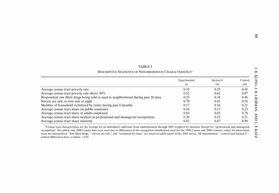
The idea that residence in a distressed community can limit an individual’seconomic prospects was advanced by Wilson (1987), and the related hypothe-sis that proximity to employment is important has its roots in the spatial mis-match hypothesis of Kain (1968). However, we found no significant evidence oftreatment effects on earnings, welfare participation, or amount of governmentassistance after an average of 5 years since random assignment. As shown inFigure 3, the fraction of MTO adults with positive quarterly UI earnings in-creased from less than 25 percent in early 1995 to more than 50 percent in2001. The time patterns are, however, similar for the three randomly assignedgroups.22

We have examined possible reasons for the lack of effects. There do not ap-pear to be important differences across the three MTO groups in job accessibil-ity, to the extent that aggregate employment growth in establishments at the zipcode level reflects available job vacancies (Web Appendix, Table F14).23 TheMTO intervention also had only small impacts on job-related social networks.Although the intervention modestly increased the fraction of sample memberswho “had a friend who graduated from college or earned more than $30,000 ayear,” only about 8 percent of the sample “found a job through someone liv-ing in their neighborhood such as a friend, relative, or acquaintance,” and this

22The strong U.S. labor market, welfare reform, and declining share of sample members withpreschool-age children are the most likely explanations for this upward trend. In analyses shownin Web Appendix, Tables F3 and F4, we found similar results based on survey and administrativedata, suggesting little bias in self-reports.

23It may be surprising that the MTO intervention—which assisted families to move out ofsome of the most concentrated pockets of U.S. poverty—had no discernable overall effects onemployment, given a recent survey (Ihlandfeldt and Sjoquist (1998)) that concluded the evidencesupports the spatial mismatch hypothesis that inner-city low-skilled minority workers have weakaccess to jobs because job opportunities are disproportionately in suburban areas and housingmarket discrimination plus commuting costs prevent minorities from reaching suburban jobs.However, the MTO experiment provides only a weak test of this view of spatial mismatch be-cause the effects on distance moved and on local area job growth are small. If spatial mismatchis broadly construed to encompass how residence in distressed, crime-ridden communities mayinhibit job access, the results indicate that moving to communities that are much safer does nothave detectable effects on employment.


FIGURE 3.—Employment rates over time. Employment is the fraction with positive earningsper quarter from Unemployment Insurance records in California, Illinois, Maryland, Massa-chusetts, and New York.

proportion did not vary across MTO groups (Web Appendix, Table F10). Insubsequent follow-up work based on 67 semistructured open-ended interviewswith MTO adults, Turney et al. (2006) found that transportation difficultiesand disrupted social networks were additional barriers to employment in theexperimental group.

We also explored whether effects differed by baseline characteristics: in gen-eral, results do not differ appreciably by these characteristics.24 However, inresults shown in the Web Appendix, Tables F7 and F8, we find suggestive ev-idence using administrative UI data of interesting dynamics in the treatmenteffects on employment and earnings for younger adults (those younger than33 years at random assignment): initial negative treatment effects in the first2 years after random assignment fade away over time for the Section 8 groupand turn positive and substantial in the fourth and fifth years after randomassignment for the experimental group.25

24Economic self-sufficiency results by age are given in the Web Appendix, Tables F6–F8. Re-sults for other household head characteristics and by gender composition of the household areavailable from the authors.

25Examining effects by age was an exploratory, not a confirmatory, exercise. This type ofsearching for significant effects in subgroups raises the chance of concluding that there are statis-tically significant results even when the null hypothesis of no effects is true.


Adult Physical Health

Our early work at the Boston site (Katz, Kling, and Liebman (2001)) sug-gested that the MTO intervention may have had important health impactsand led us to expand the outcomes studied beyond the economic and hous-ing outcomes that were the original focus of the MTO demonstration. In themuch more extensive health data gathered in the current study, there was nobroad pattern of physical health improvements for the treatment groups. Theintervention did not have statistically significant effects on self-reported overallhealth, hypertension, asthma, or trouble carrying groceries or climbing stairs,and there was not a statistically significant effect on the physical health indexin Table II.26

There was a large and statistically significant effect on obesity (see Table III),possibly related to the reduced psychological distress and increase in exerciseand nutrition that we also observed for the treatment groups. The interpreta-tion of the obesity results depends largely on one’s reason for focusing on obe-sity. If a researcher was searching for social experiments about the effects ofneighborhoods on obesity (and this is the only one), focusing on the t-statisticof 2.2 and the associated per-comparison p-value of 0.03 is highly suggestive ofan important effect of residential location on obesity. If a researcher is search-ing the MTO results for significant effects, however, we suggest some cautionin interpreting the obesity results. When using a method that focuses on partic-ular results from among many outcomes of a family because of their t-statistics,there is considerable likelihood that the obesity results could have been ob-served by chance under a joint null hypothesis of no effects for all estimates inthat family.27

Adult Mental Health

In contrast to the results for physical health, the adult mental health resultswere quite consistent across specific measures (distress, depression, anxiety,calmness, and sleep) in finding beneficial effects for the experimental group

26Analyses by age show a positive and significant impact of the MTO experimental treatmenton our summary measure of physical health outcomes for the younger adults and no significantoverall impact for older adults. These health impacts come from aggregating five consistentlysigned estimates with small magnitudes rather than from a large effect on any one measure (WebAppendix, Table F6). This result, along with the suggestive evidence of employment gains amongyounger adults, leads us to speculate that the habits and behaviors of younger adults may be moremalleable and, therefore, more responsive to a change in residential environment.

27The probability that the second largest t-statistic among 30 adult estimates is 2.2 or higherunder the joint null hypothesis of no effect is a familywise adjusted p-value of 0.80, which isindicative of the fact that there is little power to reject the joint null hypothesis for specific out-comes. The adjusted p-values throughout this paper are based on a bootstrap procedure that ac-counts for covariance among estimates, using a method adapted from Westfall and Young (1993)as described in Appendix B of the Web Appendix.


relative to the control group. This consistency led to the large mean (ITT) ef-fect size estimate of 0.08 standard deviations for the adult mental health sum-mary measure in Table II. The confidence level that the results are not due tochance is quite high under a method where the focus on mental health is de-termined exogenously (leading to per-comparison inference) or endogenouslyfrom the high t-statistic (leading to familywise inference).28 The magnitude ofthe mental health results—for example, a 45 percent reduction in relative riskamong compliers of scoring above the K6 screening cut point for serious men-tal illness (Kessler et al. (2003))—is comparable to that found in some of themost effective clinical and pharmacologic mental health interventions.29

The overall pattern of adult results—with the agreement of estimated effectsbased on self-reports and administrative records of economic outcomes, withthe effects concentrated in the single domain of mental health, and with themental health effect sizes systematically related to changes in neighborhoodpoverty rates in Figure 2A and in Table IV—indicates that there are benefi-cial impacts on mental health of moving to less distressed neighborhoods. Inaddition, this pattern is contrary to a model in which the unrestricted choiceof the Section 8 group should have led to better outcomes than the restrictedchoice of the experimental group. Based in part on evidence from the exten-sive qualitative interviews that have been done with MTO participants and thestrong associations shown in the MTO quantitative research, we believe thatthe leading hypothesis for the mechanism that produces the mental health im-provements involves the reduction in stress that occurred when families movedaway from dangerous neighborhoods in which the fear of random violence in-fluenced all aspects of their lives (Kling, Liebman, and Katz (2005), Popkin,Harris, and Cunningham (2002)).

28We focus our familywise inference on the summary indices, thereby reducing the dimensionof the inference problem. For adults, we focus on eight ITT estimates for summary indices in Ta-ble II. The familywise adjusted p-value for the mental health index t-statistic being 2.8 or higher(i.e., the largest t-statistic on estimates for eight adult indices) under the joint null hypothesis ofno effect on any of the eight adult indices in Table II is 0.06.

29In a study often cited as an exemplar of an effective clinical intervention, Wells et al. (2000)analyzed outcomes of depressive patients randomized to obtain usual care or improved qualitycare (better training of medical staff and better follow-up with patients). Twelve months later,the fraction with depressive symptoms in the quality improvement group was 0.42, while the frac-tion was 0.51 in the usual care group—a reduction in relative risk of 18 percent. A metanalysisof clinical trials of medications for major depressive disorder found that on average 50 percentof patients who received active medication showed improvement compared with 29 percent whoreceived a placebo—a reduction in relative risk of 30 percent (Walsh et al. (2002)). The reduc-tion in relative risk for major depressive episode among MTO experimental compliers was also30 percent (Web Appendix, Table F5). Improved mental health for the treatment groups relativeto the control group was a mechanism that we had hypothesized might increase employment andearnings. Although the effects on mental health reported here are large, Kling, Liebman, Katz,and Sanbonmatsu (2004) calculated that these are unlikely to translate into effects on earningslarge enough to detect.


Female Youth Outcomes

Teenage youth are often seen as the population most at risk from the adverseeffects of high-poverty neighborhoods. In this study, 15 specific outcomes wereassessed for youth within the four domains of physical health, mental health,risky behavior, and education. A summary index of all 15 outcomes shows largebenefits for female youth in the experimental and Section 8 groups relative tothe control group. The pattern of beneficial effects is quite consistent acrossoutcomes: 13 of 15 outcomes have the sign of a treatment effect in a benefi-cial direction for both treatments. The magnitudes of the effects are largestfor mental health, still substantial for education and risky behavior, and smallfor physical health. For example, the experimental compliers have a relativerisk of serious generalized anxiety symptoms 70 percent lower than the controlcomplier mean.

To assess statistical significance, we adopt a framework similar to that usedfor adult outcomes. If there is ex ante interest by a researcher in a particu-lar estimate, then the per-comparison p-value for that estimate is appropri-ate. When considering the many estimates for youth simultaneously, there isa high probability of observing a few large estimates due to sampling variabil-ity, even if there was no true effect. To account for these multiple compar-isons while restricting the set to a manageable size, we considered inferencefor three youth subgroups (all, female, and male), two treatments (experi-mental and Section 8), and five domains (physical health, mental health, riskybehavior, education, and overall), which correspond to the 30 estimates incolumns (iii)–(viii) of Table II. We calculated familywise adjusted p-values,which are similar to Bonferroni corrections, but adjusted for the ordering ofthe tests and the covariance of the estimates as described in Appendix B ofthe Web Appendix. The estimate in this set with the largest t-statistic was theoverall summary index for the experimental group, and the probability of ob-serving an effect this large or larger as the maximum of the 30 estimates wasless than 0.001 under the joint null hypothesis of no effects for the 30 estimates.The familywise adjusted p-value was 0.003 for the experimental group mentalhealth index for female youth. Based on these calculations, we conclude thatthe overall pattern and the mental health result for the experimental groupwere quite unlikely to have occurred by chance, even if the focus was on theseresults because of their large t-statistics.

Male Youth Outcomes

The results for the overall summary index of male youth outcomes are ofalmost exactly the same magnitude as for female youth but with the oppositesign, implying more adverse effects in the treatment groups than in the controlgroup. Among specific outcomes, the effects are largest for injuries and for sub-stance use, as shown in Table III, leading to large effects for the male physicalhealth and risky behavior summary indices in Table II. These summary index


measures for males have highly significant per-comparison p-values, althoughfamilywise adjusted p-values were greater than 0.05.

There are a number of issues that complicate interpretation of the resultsfor male youth. First, males in the treatment groups exhibited more behaviorand other problems at baseline than did those in the control group (there wereno such baseline differences among females).30 This imbalance appears largelyto be due to the random sampling that occurred when we subsampled childrenfor our interviews, rather than to survey attrition or imbalance in the originalrandom assignment.31 The key question for our analysis is whether our regres-sion controls for baseline covariates are sufficient to adjust for the imbalance.We suspect that our regression adjustment is sufficient to remove most of thepotential bias. Most importantly, in analysis of administrative arrest data usingthe full set of MTO youth (with little imbalance in covariates and no surveyattrition), Kling, Ludwig, and Katz (2005) found adverse treatment effects formales and beneficial effects for females, which supports our conclusion thatgender differences in effects are substantial and not simply an artifact of sam-pling issues.

A second issue is that the rates of some adverse outcomes in the controlgroup seem implausibly low. For example, the proportion of nonsports injuriesfor male youth in the control group is barely half as high as the injury rate forfemales, whereas our analysis of National Health Interview Survey data foundnonsports injury rates for male youth over 30 percent higher than for femaleyouth. Moreover, assuming that the injury rate among control noncompliersis the same as for treatment noncompliers implies a control complier mean ofless than zero. Both of these facts are consistent with a low realization of in-jury rates for the particular sample and time period for which we have data;we speculate that the injury rate for males would be at least as high for fe-males if we were to run the experiment again. The rates of substance use for

30This result comes from a summary index of baseline covariates constructed in the same man-ner as the outcomes indices (normalizing the control group for each gender to mean 0 andstandard deviation 1). The index includes variables collected prior to random assignment forage, gifted classes, school suspension, problems at school, behavior problems, learning problems,physical activity problems, and other medical problems.

31For the following discussion, E − C and S − C refer to ITT differences in the baseline co-variate index in standard deviation units for male youth (with standard errors). For all 1,604 maleyouth ages 15–20 in MTO households, the E − C difference was −0�022 (0.031) and the S − Cdifference was −0�019 (0.034). For the 923 male youth we attempted to survey (drawing two chil-dren per household and a 3-in-10 subsample of initial nonrespondents), the E − C difference was−0�133 (0.053) and the S − C difference was −0�108 (0.055). For the 879 youth with whom wecompleted surveys, the E − C difference was −0�158 (0.054) and the S − C difference was −0�129(0.056). Because there was less than half a standard error difference, respectively, between theestimates for all male youth for whom surveys were attempted and for those completed but largeimbalance between treatment groups in baseline covariates for those attempted, we conclude thatthe imbalance was largely driven by random sampling. For comparison with the 928 female youthsurveyed, the E − C difference was −0�021 (0.044) and the S − C difference was −0�047 (0.055).


males in the control group are also low relative to demographically similar indi-viduals in national data, whereas there are smaller differences between MTOcontrols and national data for females.32 Our interpretation of the results isthat issues such as random covariate imbalance, survey attrition, and surpris-ingly low prevalence of adverse outcomes among controls may exaggerate themagnitude of the adverse effects for males, but that these factors are not largeenough to account for the differences in effects between males and females.

Understanding Gender Differences

We collected extensive data on mediating factors that could potentially helpto determine the mechanisms responsible for the gender differences in the re-sults for youth. In brief, we find that there were large effects of the treatmenton neighborhood characteristics and smaller effects on school characteristics,but no significant differences by gender in the treatment effects on neighbor-hoods or schools (see the Web Appendix, Tables G3–G7 for details).33 We con-clude that female youth and male youth in the treatment groups responded tosimilar new neighborhood environments in different ways.

Several mechanisms could potentially explain the gender differences inneighborhood effects. There has been a broad trend over the past two decadesof gains in education and employment for minority women—gains that havenot been shared by minority men (Altonji and Blank (1999)). Moves throughMTO may remove barriers to benefiting from these gains for female youth,whereas the male youth have poor prospects even in lower poverty neighbor-hoods. It is also likely that girls suffer disproportionately from domestic vi-olence and sexual abuse (Popkin, Harris, and Cunningham (2002)), and theMTO intervention may have reduced their exposure to such events, provid-ing benefits from the moves for girls that were not nearly as relevant for boys.We did find some statistically significant survey evidence that female youth aremore likely to have three or more adult role models to whom they are com-fortable talking about their problems (Web Appendix, Table G5) and that themean effect size on a summary index of adult contact measures was signifi-cantly higher for female youth than for male youth. Although the probability is

32In Appendix D of the Web Appendix, we describe our method for producing results forthe National Longitudinal Survey of Youth 1997 (NLSY97) that are adjusted to match the demo-graphics of the MTO sample. The following results in parentheses are for the MTO control group,the adjusted NLSY97, and the unadjusted NLSY97, respectively: marijuana (females: 0.13, 0.10,0.16; males: 0.12, 0.23, 0.18), cigarettes (females: 0.19, 0.25, 0.33; males: 0.13, 0.33, 0.33), and al-cohol (females: 0.21, 0.26, 0.44; males: 0.14, 0.32, 0.46). The deviations of the MTO controls fromthe adjusted NLSY97 across these three outcomes are substantially smaller for females than formales, consistent with a random draw of unusually low substance use among males in the controlgroup.

33We also find that the MTO intervention had no significant impacts on parenting practices,peer characteristics, school engagement, or access to health care for either boys or girls (WebAppendix, Tables G4–G7).


quite high of observing at least one effect this large under a joint null hypothe-sis of no gender differences in the many mediating mechanisms we examined,our interpretation is that differences in adult contact are the most likely con-tributor to at least part of the gender difference in effects from among themechanisms about which we have data to examine.34

To further develop ideas about why the gender differences in effects mighthave occurred, a qualitative research effort was designed to follow up onthe results reported in this paper. Clampet-Lundquist, Edin, Kling, and Dun-can (2006) examined data from semistructured open-ended interviews with83 youth in Chicago and Baltimore randomly selected from the MTO experi-mental and control groups. Gender differences were found in effects for out-comes collected as part of this qualitative data, complementing similar resultsfrom the 2002 survey and from administrative arrest records. Before seeingthe data, our leading hypothesis for why youth who moved to lower povertyneighborhoods might experience adverse outcomes was “relative deprivation”;for example, male youth in the experimental group could find themselves sur-rounded by relatively higher achieving peers and react negatively to being “fur-ther down the ladder.” However, the qualitative interviews did not provide anyevidence that relative deprivation was a salient experience for male youth inthe experimental group.

Clampet-Lundquist et al. did find some evidence to support several other hy-potheses. First, the nondominant cultural capital skills (e.g., use of language)that male youth learned in their high-poverty neighborhoods may have iso-lated them from the mainstream when they moved to lower poverty contexts.This cultural conflict sometimes manifested itself through police harassmentor through fear and misunderstanding, and may have led to maladaptive be-havior. Second, male youth may have experienced more negative peer effects.Male youth tended to spend their free time on neighborhood basketball courtsand on street corners, in closer proximity to illegal activity than the female

34We also found that the beneficial effects on adult mental health outcomes overall (such asdistress and calmness) were not evident for adults with male youth in their households, with thedifference for male–female youth being significant. This finding could be the effect of adversemale outcomes rather than the cause. Male youth may have less effective coping strategies instressful situations (Zaslow and Hayes (1986), Coleman and Hendry (1999), Kraemer (2000))and the disruption of moving itself may have been greater for male youth. However, at leasttwo strands of evidence run counter to this hypothesis. First, mobility rates were slightly higheramong households with female youth than those with male youth (Web Appendix, Table G8).Second, the adverse effects for males did not manifest themselves right after the initial moves, aspredicted by a simple mobility disruption model, but only after several years. In studies of singleMTO sites 1–3 years after random assignment, there were either no gender differences in effectsreported, or more beneficial effects for males than females (Katz, Kling, and Liebman (2001),Leventhal and Brooks-Gunn (2003a, 2003b)). In administrative arrest data, the adverse effectson male property crime are not found in the first two years after random assignment, but in thethird and fourth years (Kling, Ludwig, and Katz (2005)).


youth, who tended to spend free time at home or in malls or other more super-vised spaces. Many of the male youth in the control group developed strategiesof “keeping to themselves” that helped them stay out of trouble, whereas fewerexperimental group males used such strategies. Relatedly, experimental groupmales may have responded to peer pressure to signal that they had not aban-doned their origin neighborhood culture by participating in deviant activitiesand returning to the origin neighborhood.35 Third, male youth in the controlgroup had particularly high rates of contact with father figures (stepfathers,mother’s boyfriends, and uncles), likely contributing to the differential adultcontact effects observed in the survey. In the qualitative study, rates of contactwith biological fathers were similar for all groups and genders, and the preva-lence of important contact with other adults outside of the family was also lowfor all.

Reconciling OLS and 2SLS Estimates

If low neighborhood poverty rates were beneficial and the neighborhood se-lection process operated such that people with unobserved characteristics asso-ciated with good outcomes tended to locate in lower poverty neighborhoods,these assumptions would predict that the OLS estimates of effects of higherpoverty rates would be more adverse than 2SLS estimates using site–treatmentgroup interactions as instruments for neighborhood poverty. In Table IV, how-ever, we found OLS estimates (based on the control group only) that wereoften of opposite sign from 2SLS (for the full sample). The implied selectionprocess is that adults and families with female teenagers likely to have ad-verse outcomes tended to move to low poverty neighborhoods, and familieswith male teenagers likely to have beneficial outcomes tended to move to low-poverty neighborhoods.36 These selection patterns suggest that identifying thedirection of bias in nonexperimental studies of neighborhood effects can bemore complex than is typically assumed.

35According to our survey data, male experimental group youth did make more visits to theirorigin neighborhoods than did females, but the male–female difference is insignificant (Web Ap-pendix, Table G5). For males, a two-audience signaling process (Austen-Smith and Fryer (2005))could encourage them to avoid peer sanction through participation in deviant group activi-ties rather than engage in more prosocial behaviors that are ultimately valued by employers—a process that could be more important when there is more uncertainty about social group affili-ation due to greater racial, ethnic, or economic diversity among peers (as there would tend to befor youth in families using MTO vouchers). Fryer and Torelli (2005) find some evidence consistentwith greater peer sanction against prosocial activities of black males than those of females.

36These implications about the pattern of residential sorting are borne out within the treatmentgroups as well. For nearly all outcomes, the compliers are more similar to the noncompliers thanto the control group. For female youth and adults, this pattern can only be consistent with benefi-cial treatment effects if compliers otherwise would have had poor outcomes. For male youth, thispattern can only be consistent with adverse treatment effects if compliers otherwise would havehad good outcomes.


Younger Children

Sanbonmatsu et al. (2006) hypothesized that greater effects of the MTOtreatment would be found on children who are younger than the youth whoseoutcomes we study in this paper because the younger children (such as thoseages 6–10) will have had less lifetime exposure to the high-poverty neighbor-hoods, but they found no statistically significant treatment effects for youngerchildren on reading test scores, math test scores, or behavior problems. How-ever, the main outcomes for which we found large treatment effects for teenageyouth—mental health problems and risky behavior—have very low prevalenceat younger ages, and it is therefore too early to tell whether the outcomes ofthe younger children will be different.

4. CONCLUSION

Using a housing voucher lottery that caused otherwise similar groups of fam-ilies to reside in very different neighborhoods, we have investigated the effectsof moving out of some of the highest poverty neighborhoods in the UnitedStates on outcomes for adults and teenage youth. Our findings—no discern-able effects on adult economic self-sufficiency, improvements in adult men-tal health, beneficial outcomes for teenage girls, and adverse outcomes forteenage boys—have three important implications.

First, housing mobility by itself does not appear to be an effective antipovertystrategy—at least over a 5-year horizon. The MTO demonstration program wasmotivated by theories and nonexperimental empirical results that suggestedthat there would be large economic gains from moving to lower poverty neigh-borhoods. However, we found no consistent evidence of treatment effects onadult earnings or welfare participation. Whether economic gains begin to ap-pear in the longer run, particularly among MTO children, remains to be seen.

Second, even in the absence of economic gains, policies that move familiesout of distressed public housing projects using rental vouchers are likely tohave benefits that significantly exceed their costs. Because the MTO interven-tion produced large mental health improvements and because other researchsuggests that it is cheaper to provide a unit of subsidized housing with vouchersthan in a public housing project (Olsen (2000)), an offer of a housing voucheris likely to pass the Kaldor–Hicks criterion—the gains to those who benefitwould be large enough to hypothetically compensate those who experience ad-verse effects and still leave those who benefit better off. We note, however, thatspillovers onto neighborhoods to which these families moved remain unknown.If there were large negative spillovers, this conclusion could be reversed. Inaddition, the largely offsetting male and female youth results complicate thewelfare analysis.

Third, substantively important neighborhood effects do exist, but only forsome outcomes. Teenagers—the population often thought to be most affected


by neighborhood conditions—exhibited effects on the broadest range of out-comes. The evidence that the effects of housing vouchers appear to accruefrom changes in neighborhood characteristics rather than from moves perse suggests that interventions that substantially improve distressed neighbor-hoods could have effects as least as large as those observed from moving tolower poverty neighborhoods.37 Although numerous nonexperimental studiesdocument strong associations between neighborhood characteristics and indi-vidual outcomes, these associations appear to be much weaker in the studieswith the most credible identification strategies.38 Because the current studyused randomization to solve the selection problem, because it studied fam-ilies who made very large moves as measured by changes in neighborhoodpoverty rates, and because it collected extensive data on teenagers, it providesus with the clearest answer so far to the threshold question of whether impor-tant neighborhood effects exist.

The Brookings Institution, 1775 Massachusetts Ave., NW, Washington, DC20036, U.S.A.; [email protected], www.brookings.edu/scholars/jkling.htm,

John F. Kennedy School of Government, Harvard University, 79 JFKStreet, Cambridge, MA 02138, U.S.A.; [email protected], www.jeffreyliebman.com,

andDept. of Economics, Harvard University, Littauer Center, Cambridge, MA

02138, U.S.A.; [email protected], post.economics.harvard.edu/faculty/katz/katz.html.

Manuscript received May, 2004; final revision received June, 2006.

APPENDIX A: DESCRIPTION OF BASELINE COVARIATES AND OUTCOMES

The covariates (X) used in Equations (1)–(3) were drawn from data col-lected in a baseline survey conducted prior to random assignment. For analysisof adults, the covariates were those in Table A1 and six Legendre polynomialsfor adult date of birth. For analysis of youth, all the covariates in Table A1 wereused as well as those in Table A2, six Legendre polynomials for youth date ofbirth, and five indicators for missing data on special class for gifted students ordid advanced work, special school, class, or help for learning problem in pasttwo years, special school, class, or help for behavioral or emotional problemsin past two years, problems that made it difficult for him/her to get to school

37Bloom, Riccio, and Verma (2005) found substantial positive earnings effects in a community-based intervention.

38For example, Ellen and Turner (1997) report that “some recent studies that have done themost careful job of controlling for unobserved family characteristics � � � find no independentneighborhood effects, casting doubt on the robustness of results from other studies.” Also, recentquasi-experimental studies (Jacob (2004), Oreopoulos (2003)) find little or no effect of living inhigh-poverty housing projects on child outcomes.

mailto:[email protected]

http://www.brookings.edu/scholars/jkling.htm


http://www.jeffreyliebman.com


http://post.economics.harvard.edu/faculty/katz/katz.html

http://www.jeffreyliebman.com

http://post.economics.harvard.edu/faculty/katz/katz.html

110J.R

.KL

ING

,J.B.L

IEB

MA

N,A

ND

L.F.K

AT

Z

TABLE A1

ADULT BASELINE CHARACTERISTICSa

ControlMean

Experimental Section 8

Mean CP Mean NCP Mean CP−NCP Mean CP Mean NCP Mean CP−NCPVariable (i) (ii) (iii) (iv) (v) (vi) (vii) (viii) (ix)

DemographicsAge in years (as of

December 2001) 39.6 39.7 38.1 41.2 −3.1∗ 40.1 38.3 42.6 −4.2∗

Male 0.02 0.01 0.00 0.02 −0.01∗ 0.02 0.02 0.02 0.00Baltimore site 0.15 0.15 0.17 0.13 0.04 0.15 0.18 0.10 0.09∗

Boston site 0.21 0.22 0.21 0.22 −0.02 0.22 0.18 0.28 −0.10∗

Chicago site 0.22 0.23 0.16 0.30 −0.14∗ 0.23 0.25 0.19 0.06Los Angeles site 0.16 0.16 0.21 0.10 0.11∗ 0.15 0.19 0.09 0.11∗

New York site 0.25 0.25 0.25 0.24 0.01 0.25 0.19 0.34 −0.15∗

African–American 0.66 0.67 0.67 0.66 0.01 0.66 0.70 0.60 0.10∗

Other race 0.27 0.26 0.23 0.29 −0.05∗ 0.26 0.22 0.31 −0.09∗

Hispanic ethnicity, anyrace 0.29 0.29 0.28 0.29 −0.02 0.30 0.27 0.35 −0.08∗

Never married 0.62 0.62 0.66 0.58 0.08∗ 0.62 0.65 0.58 0.07Teen parent 0.24 0.25 0.26 0.24 0.02 0.26 0.30 0.21 0.08∗

Economic and educationWorking 0.25 0.29 0.29 0.28 0.02 0.25 0.26 0.24 0.03On AFDC 0.75 0.74 0.76 0.72 0.04 0.75 0.78 0.70 0.08∗

In school 0.16 0.16 0.20 0.12 0.07∗ 0.16 0.18 0.12 0.05∗

High school diploma 0.38 0.41 0.41 0.42 −0.01 0.41 0.41 0.40 0.01General equivalency

diploma 0.21 0.18 0.21 0.15 0.06∗ 0.19 0.20 0.18 0.01

Continues

NE

IGH

BO

RH

OO

DE

FF

EC

TS

111

TABLE A1—Continued

ControlMean



HouseholdHad car 0.15 0.17 0.19 0.15 0.04 0.16 0.18 0.14 0.05Household member with a

disability 0.16 0.16 0.15 0.17 −0.02 0.17 0.14 0.20 −0.06∗

Household membervictimized by crimeduring past 6 months 0.41 0.42 0.46 0.39 0.07∗ 0.43 0.45 0.39 0.05

No teen children 0.62 0.59 0.66 0.53 0.13∗ 0.61 0.67 0.52 0.15∗

Household of size 2 0.20 0.23 0.27 0.19 0.09∗ 0.21 0.23 0.18 0.05Household of size 3 0.32 0.30 0.31 0.30 0.01 0.31 0.30 0.31 −0.01Household of size 4 0.22 0.23 0.23 0.24 −0.01 0.23 0.23 0.22 0.00

Neighborhood and housingLived in neighborhood 5

or more years 0.62 0.61 0.60 0.62 −0.02 0.63 0.57 0.72 −0.15∗

Moved more than 3 timesin past 5 years 0.11 0.08+ 0.09 0.07 0.02 0.09 0.11 0.06 0.05∗

Very dissatisfied withneighborhood 0.46 0.46 0.52 0.41 0.11∗ 0.47 0.52 0.39 0.13∗

Streets very unsafe atnight 0.49 0.48 0.52 0.45 0.07∗ 0.49 0.53 0.43 0.10∗

Chats with neighbors atleast once a week 0.55 0.52 0.49 0.55 −0.06∗ 0.50 0.50 0.50 0.00

Continues

112J.R

.KL

ING

,J.B.L

IEB

MA

N,A

ND

L.F.K

AT

Z

TABLE A1—Continued

ControlMean



Neighborhood and housing (continued)Respondent very likely to

tell neighbor if sawneighbor’s childgetting into trouble 0.56 0.53 0.50 0.57 −0.07∗ 0.55 0.56 0.53 0.03

No family living inneighborhood 0.65 0.65 0.66 0.64 0.02 0.62 0.63 0.60 0.03

No friends living inneighborhood 0.41 0.40 0.43 0.38 0.05 0.38 0.40 0.34 0.06

Very sure would find anapartment in anotherpart of city 0.45 0.45 0.51 0.40 0.11∗ 0.48 0.54 0.40 0.14∗

To get away from gangsor drugs was primaryor secondary reasonfor moving 0.78 0.77 0.79 0.75 0.04 0.75 0.77 0.73 0.05

Better schools wasprimary or secondaryreason for moving 0.48 0.47 0.50 0.46 0.04 0.52 0.53 0.49 0.05

Had applied for Section 8voucher before 0.45 0.41 0.44 0.39 0.05 0.39+ 0.38 0.40 −0.03

N 1,080 1,453 694 759 993 585 408aAFDC, Aid to Families with Dependent Children; CP, complier; NCP, noncomplier; *, difference between treatment compliers and noncompliers is statistically significant at

the 5 percent level; +, difference between treatment and control mean is statistically significant at 5 percent level.


TABLE A2

YOUTH BASELINE CHARACTERISTICSa

Female Male

Exp Sec8 Con Exp Sec8 Con(1) (2) (3) (4) (5) (6)

African–American 0.68 0.64 0.67 0.64 0.65 0.59Special class for gifted students or did

advanced work 0.15 0.17 0.17 0.17∗ 0.15∗ 0.27Special school, class, or help for learning

problem in past 2 years 0.13 0.13 0.12 0.29 0.25 0.30Special school, class, or help for behavioral

or emotional problems in past 2 years 0.07 0.08 0.05 0.18 0.17 0.11Problems that made it difficult to get to

school and/or to play active games 0.03 0.06 0.06 0.11∗ 0.08 0.05Problems that required special medicine

and/or equipment 0.05 0.07 0.05 0.13 0.14 0.09School asked to talk about problems child

having with schoolwork or behaviorin past 2 years 0.19 0.23 0.19 0.41 0.37 0.33

Suspended or expelled from school in past2 years 0.09 0.10 0.07 0.23 0.20 0.15

aExp, experimental; Sec8, Section 8; Con, control; *, p-value < 0�05 on difference between experimental or Sec-tion 8 and control group. Baseline data were collected at random assignment, during 1994–1997. Surveys were com-pleted in experimental, Section 8, and control groups with 749, 510, and 548 respondents, respectively, ages 15–20 on12/31/2001 for a total sample size of 1,807.

and/or to play active games or sports, and suspended or expelled from schoolin past two years.

Descriptions of the 15 outcomes examined for adults and the 15 examinedfor youth follow:

Adult economic self-sufficiency. Our measure of employment is an indicatorfor whether the adult had worked for pay during the week prior to survey.

Welfare receipt is measured as being a beneficiary of Temporary Assistancefor Needy Families (TANF) at the time of the survey.

Economic self-sufficiency is an indicator for working for pay during the pre-vious week and not receiving TANF.

Earnings in 2001 is the amount self-reported to have been earned from allemployers before taxes and deductions during 2001.

Government income is the amount received altogether in the form of TANF,Supplemental Security Income (SSI), unemployment benefits, Social Security,General Assistance, and related programs in 2001.

Adult physical health. To assess overall health, respondents were asked, “Ingeneral is your health excellent, very good, good, fair, or poor?” The analysesexamined whether the respondent reported that he or she was in fair or poorhealth.


Our measure of physical limitation was whether the respondent reportedhaving at least a little trouble “lifting or carrying groceries” or “climbing sev-eral flights of stairs.”

Respondents were asked questions from the National Health Interview Sur-vey sequence on asthma or wheezing attacks. As our dichotomous measure, weexamined the fraction of respondents who had an attack during the past year.

Subjects self-reported their height and weight. We use the standard defini-tion of obesity, BMI ≥ 30 kg/m2 (National Institutes of Health (1998)).

Our measure of hypertension is based on the JNC7 stage 1 systolic and dias-tolic blood pressure cut-points: systolic ≥140 mm HG or diastolic ≥90 mm HG(Chobanian et al. (2003)). Systolic and diastolic blood pressures were mea-sured from a single reading near the end of the survey from an OmronHEM-737. This device satisfied the American Association for the Advance-ment of Medical Instrumentation standards for accuracy (Anwar et al. (1998)).Subjects were seated and had been at rest for at least 30 minutes.

Adult mental health. Distress during the past 30 days was assessed using theK6 scale, developed by Kessler et al. (2002). This scale score can range from 0to 24, which we normalize to a z-score by subtracting the mean of 5.8 anddividing by the standard deviation of 5.4.

Depression was assessed using the Composite International DiagnosticInterview—Short Form (CIDI-SF; Kessler et al. (1998)). If during a 2-weekperiod in the past year the respondent reported dysphoric mood (feeling “sad,blue, or depressed”) or anhedonia (having “lost interest in most things”),then he or she was assigned a probability of having had a major depressiveepisode (MDE) according to the number endorsed of seven possible symptomsthat correspond to those used for Diagnostic and Statistical Manual of MentalDisorders, Fourth Edition (DSM-IV) psychiatric diagnosis. The probability isbased on a mapping between the CIDI-SF screening questions and more de-tailed assessments in the National Comorbity Survey (Walters, Kessler, NelsonChristopher, and Mroczek (2002)).

For worrying, respondents were asked the two initial screening items fromthe CIDI-SF sequence on generalized anxiety disorder, and we analyzed thefraction of the sample who answered “yes” to “felt worried, tense, or anxious”or “worried a lot more than most people would in your situation” (Kessler et al.(1998)).

Respondents were asked if they felt “calm and peaceful” at least most of thetime during the past month—one of the items from the mental health inventoryin the RAND Health Insurance Experiment and the Short Form-36 (Ware,Snow, Kosinski, and Gandek (1993)).

Sleep was measured as the amount of time that participant usually spentsleeping each night, and we analyzed the fraction that usually sleep at least 7and less than 9 hours per night.

Youth education. Our measure of whether a youth had graduated from highschool or was still in school is based on a parental report.


To assess idleness, we asked youth whether they were in school, on summervacation from school, working during the past week, or none of the above.

Reading achievement was assessed using the Woodcock–Johnson Revised(WJ-R) Broad Reading assessment, which includes letter–word identificationand passage comprehension subtests.

Math achievement was assessed using the Woodcock–Johnson Revised(WJ-R) Broad Math assessment, which includes applied problems and cal-culation subtests. As discussed in Sanbonmatsu et al. (2006), some systematicdifferences in scores on tests administered by particular interviewers were de-tected for reading and math tests, and the results presented in Table III areadjusted for interviewer effects after controlling for census tract fixed effects.

Youth physical health. Our analysis of youth health is based on self-reportedinformation in response to questions drawn mainly from the National HealthInterview Survey about general health status, injuries, asthma attacks, height,and weight. Case, Lubotsky, and Paxson (2002) and Currie and Stabile (2003)find that self-reported poor health correlates strongly with children’s chronicconditions, bed days, and hospitalization episodes.

For asthma attacks, we follow the standard practice of combining attacksrequiring medical attention with other episodes of wheezing or whistling in thechest (Pearce, Beasley, Burgess, and Crane (1998)).

We asked for details of any injuries, accidents, or poisonings that requiredmedical attention or were serious enough to limit activities during the previous12 months, and we focused our analysis on nonsports injuries.

To assess obesity, we collected self-reported height and weight and calcu-lated the body mass index for each individual. Our measure of obesity is bodymass index greater than the 95th percentile of the national norms for theyouth’s age and gender.

Youth mental health. Our distress measure, developed by Kessler et al. (2002)for the National Health Interview Survey, is commonly scored by summingthe scale scores of the items, with the total ranging from 0 to 24. This mea-sure is commonly known as the K6 and is based on a six-item Likert scalethat measures how much of the time during the past 30 days the youth felt“so depressed nothing could cheer you up,” “nervous,” “restless or fidgety,”“hopeless,” “everything was an effort,” or “worthless.” Our results are reportedas z-scores, scaling by the standard deviation. The sample mean is 5.0 and thestandard deviation is 4.7.

Our measure of serious depression involved a series of screening questionsabout the duration and intensity of the feelings and the presence of relatedsymptoms during the worst period in life. A youth is considered to have had amajor depressive episode during his or her lifetime if he or she met the follow-ing five conditions:

A. The youth experienced a period in which for most of the day he or shefelt one of the following: sad, empty or depressed, very discouraged or hopelessabout how things were going in his or her life, or loss of interest and boredomwith most things usually enjoyed like work, hobbies, and personal relationships.


B. Either felt this way most of the day almost every day for a period of2 weeks or longer, or for a period of 3 days or longer and had a year or morein life when felt this way just about every month for several days or longer.

C. During times when mood was most severe and frequent, the feelings usu-ally lasted not less than 3 hours a day.

D. These feelings were either more than mild, sometimes felt so bad thatnothing could cheer him or her up, or sometimes felt so bad that he or shecould not carry out daily activities.

E. These feelings were accompanied by changes in sleeping, eating, energy,his or her ability to keep mind on things, feeling badly about his or herself, orother problems.

Our measure of anxiety also involved a series of screening questions aboutthe duration and intensity of the feelings and the presence of related symptomsduring the worst period in life. A youth was considered to have had generalizedanxiety disorder during his or her lifetime if the following four criteria weremet:

A. The youth reported there was a period when he or she was either worry-ing a lot more about things than other people with the same problems, muchmore nervous or anxious than most people with the same problems, or anxiousor worried most days.

B. The youth reported being worried about nothing in particular, every-thing, or more than one specific thing.

C. The youth sometimes or often either found it hard to stop the worries oranxiety or could not think about anything else no matter how hard he or shetried.

D. The period of being anxious, nervous, or worried lasted at least onemonth.

Youth risky behavior. Our measures of risky behavior drew upon survey self-reports using items from the National Longitudinal Survey of Youth 1997.

Alcohol use was measured as any use within the past 30 days.Marijuana use was measured as any use within the past 30 days.Smoking was measured as any cigarette smoking within the past 30 days.Our measures of whether a female youth had borne a child or a male youth

had fathered a child were also based on self-reported responses to survey ques-tions.

REFERENCES

ALTONJI, J., AND R. BLANK (1999): “Race and Gender in the Labor Market,” in Handbook ofLabor Economics, Vol. 3C, ed. by O. Ashenfeleter and D. Card. Amsterdam: North-Holland,3143–3260.

ANGRIST, J. D., G. W. IMBENS, AND D. B. RUBIN (1996): “Identification of Causal Effects UsingInstrumental Variables,” Journal of the American Statistical Association, 91, 444–472.

ANWAR, Y. A., S. GIACCO, E. J. MCCABE, B. E. TENDLER, AND W. B. WHITE (1998): “Evaluationof the Efficacy of the Omron HEM-737 Intellisense Device for Use on Adults According to the

http://www.e-publications.org/srv/ecta/linkserver/setprefs?rfe_id=urn:sici%2F0012-9682%28200701%2975%3A1%3C83%3AEAONE%3E2.0.CO%3B2-Z


Recommendations of the Association for Advancement of Medical Instrumentation,” BloodPressure Monitoring, 3, 261–265.

ARNOTT, R., AND J. ROWSE (1987): “Peer Group Effects and Educational Attainment,” Journalof Public Economics, 32, 287–305.

AUSTEN-SMITH, D., AND R. FRYER (2005): “An Economic Analysis of Acting White,” QuarterlyJournal of Economics, 120, 551–583.

BECKER, G., AND K. M. MURPHY (2000): Social Economics. Chicago: University of ChicagoPress.

BENABOU, R. (1993): “Workings of a City: Location, Education, and Production,” Quarterly Jour-nal of Economics, 108, 619–652.

BLOOM, H. S., J. A. RICCIO, AND N. VERMA (2005): Promoting Work in Public Housing: TheEffectiveness of Jobs-Plus. New York: MDRC.

BOS, J., T. BROCK, G. DUNCAN, R. GRANGER, A. HUSTON, AND V. LLOYD (1999): New Hope forPeople with Low Incomes: Two-Year Results of a Program to Reduce Poverty and Reform Welfare.New York: MDRC.

BROCK, W. A., AND S. N. DURLAUF (2001): “Interactions-Based Models,” in Handbook of Econo-metrics, Vol. 5, ed. by J. J. Heckman and E. Leamer. Amsterdam: North-Holland, 3297–3380.

BROOKS-GUNN, J., G. J. DUNCAN, AND L. ABER (1997): Neighborhood Poverty: Context and Con-sequences for Children, Vol. I. New York: Russell Sage Foundation.

CASE, A. C., D. LUBOTSKY, AND C. H. PAXSON (2002): “Economic Status and Health in Child-hood: The Origins of the Gradient,” American Economic Review, 92, 1308–1334.

CHOBANIAN, A. V., G. L. BAKRIS, H. R. BLACK, W. C. CUSHMAN, L. A. GREEN, J. L. IZZO JR.,D. W. JONES, B. J. MATERSON, S. OPARIL, J. T. WRIGHT JR., AND E. J. ROCCELLA (2003):“The Seventh Report of the Joint National Committee on Prevention, Detection, Evaluation,and Treatment of High Blood Pressure: The JNC 7 Report,” Journal of the American MedicalAssociation, 289, 2560–2572.

CLAMPET-LUNDQUIST, S., K. EDIN, J. R. KLING, AND G. J. DUNCAN (2006): “Moving At-RiskYouth Out of High-Risk Neighborhoods: Why do Girls Fare Better than Boys?” Working Pa-per, Industrial Relations Section, Princeton University.

COLEMAN, J., AND L. B. HENDRY (1999): The Nature of Adolescence. London: Routledge.CRANE, J. (1991): “The Epidemic Theory of Ghettos and Neighborhood Effects on Dropping out

and Teenage Childbearing,” American Journal of Sociology, 96, 1226–1259.CURRIE, J., AND M. STABILE (2003): “Socioeconomic Status and Health: Why Is the Relationship

Stronger for Older Children?” American Economic Review, 93, 1813–1823.DAVIDSON, R., AND J. G. MACKINNON (1993): Estimation and Inference in Econometrics. New

York: Oxford University Press.DE BARTOLOME, C. (1990): “Equilibrium and Inefficiency in a Community Model with Peer Ef-

fects,” Journal of Political Economy, 98, 100–113.ELLEN, I. G., AND M. A. TURNER (1997): “Does Neighborhood Matter? Assessing the Recent

Evidence,” Housing Policy Debate, 8, 833–866.ENTWISLE, D. R., K. L. ALEXANDER, AND L. S. OLSON (1994): “The Gender Gap in Math: Its

Possible Origins in Neighborhood Effects,” Child Development, 67, 2400–2416.FERNANDEZ, R., AND R. ROGERSON (1996): “Income Distribution, Communities and the Quality

of Public Education,” Quarterly Journal of Economics, 111, 135–164.FRYER, R., AND P. TORRELLI (2005): “An Empirical Analysis of Acting White,” Unpublished

Manuscript, Harvard University.GOERING, J. M., AND J. D. FEINS (eds.) (2003): Choosing a Better Life: Evaluating the Moving to

Opportunity Social Experiment. Washington, DC: Urban Institute Press.GRANOVETTER, M. (1978): “Threshold Models of Collective Behavior,” American Journal of So-

ciology, 83, 1420–1443.HECKMAN, J. J. (1990): “Varieties of Selection Bias,” American Economic Review, 80, 313–318.

(2001): “Accounting for Heterogeneity, Diversity and General Equilibrium in Evaluat-ing Social Programs,” Economic Journal, 111, 654–699.


IHLANFELDT, K. R., AND D. J. SJOQUIST (1998): “The Spatial Mismatch Hypothesis: A Review ofRecent Studies and Their Implications for Welfare Reform,” Housing Policy Debate, 9, 849–892.

IMBENS, G. W., AND J. D. ANGRIST (1994): “Identification and Estimation of Local AverageTreatment Effects,” Econometrica, 62, 467–475.

JACOB, B. A. (2004): “Public Housing, Housing Vouchers, and Student Achievement: Evidencefrom Public Housing Demolitions in Chicago,” American Economic Review, 94, 233–258.

JENCKS, C., AND S. E. MAYER (1990): “The Social Consequences of Growing up in a Poor Neigh-borhood,” in Inner City Poverty in the United States, ed. by L. Lynn Jr. and M. McGeary. Wash-ington, DC: National Academy Press, 111–186.

KAIN, J. F. (1968): “Housing Segregation, Negro Employment and Metropolitan Decentraliza-tion,” Quarterly Journal of Economics, 82, 175–197.

KATZ, L. F., J. R. KLING, AND J. B. LIEBMAN (2001): “Moving to Opportunity in Boston: EarlyResults of a Randomized Mobility Experiment,” Quarterly Journal of Economics, 116, 607–654.

KAWACHI, I., AND L. F. BERKMAN (2003): “Introduction,” in Neighborhoods and Health, ed. byI. Kawachi and L. F. Berkman. Oxford: Oxford University Press, 1–19.

KESSLER, R. C., G. ANDREWS, L. J. COLPE, E. HIRIPI, D. K. MROCZEK, S. T. NORMAND,E. E. WALTERS, AND A. M. ZASLAVSKY (2002): “Short Screening Scales to Monitor Popu-lation Prevalences and Trends in Non-Specific Psychological Distress,” Psychological Medicine,32, 959–976.

KESSLER, R. C., G. ANDREWS, D. K. MROCZEK, T. B. USTUN, AND H. U. WITTCHEN (1998):“The World Health Organization Composite International Diagnostic Interview Short-Form(CIDI-SF),” International Journal of Methods in Psychiatric Research, 7, 171–185.

KESSLER, R. C., P. R. BARKER, L. J. COLPE, J. F. EPSTEIN, J. C. GFROERER, E. HIRIPI,M. J. HOWES, S. T. NORMAND, R. W. MANDERSHEID, E. E. WALTERS, AND A. M. ZASLAVSKY(2003): “Screening for Serious Mental Illness in the General Population,” Archives of GeneralPsychiatry, 60, 184–189.

KLING, J. R., AND J. B. LIEBMAN (2004): “Experimental Analysis of Neighborhood Effects onYouth,” Working Paper 483, Industrial Relations Section, Princeton University.

KLING, J. R., J. B. LIEBMAN, AND L. F. KATZ (2005): “Bullets Don’t Got No Name: Conse-quences of Fear in the Ghetto,” in Discovering Successful Pathways in Children’s Development:New Methods in the Study of Childhood and Family Life, ed. by T. S. Weisner. Chicago: Univer-sity of Chicago Press, 243–281.

(2007): “Supplement to ‘Experimental Analysis of Neighborhood Effects’,” Economet-rica Supplementary Material, 75, http://www.econometricsociety.org/ecta/supmat/tables.pdf.

KLING, J. R., J. B. LIEBMAN, L. F. KATZ, AND L. SANBONMATSU (2004): “Moving to Opportunityand Tranquility: Neighborhood Effects on Adult Economic Self-Sufficiency and Health from aRandomized Housing Voucher Experiment,” Working Paper 481, Industrial Relations Section,Princeton University.

KLING, J. R., J. LUDWIG, AND L. F. KATZ (2005): “Neighborhood Effects on Crime for Femaleand Male Youth: Evidence from a Randomized Housing Voucher Experiment,” Quarterly Jour-nal of Economics, 120, 87–130.

KRAEMER, S. (2000): “The Fragile Male,” British Medical Journal, 321, 23–30.LEVENTHAL, T., AND J. BROOKS-GUNN (2003a): “Moving to Opportunity: An Experimental

Study of Neighborhood Effects on Mental Health,” American Journal of Public Health, 93,1576–1582.

(2003b): “New York City Site Findings: The Early Impacts of Moving to Opportunityon Children and Youth,” in Choosing a Better Life: Evaluating the Moving to Opportunity SocialExperiment, ed. by J. M. Goering and J. D. Feins. Washington, DC: The Urban Institute Press,213–244.

LIEBMAN, J. B., L. F. KATZ, AND J. R. KLING (2004): “Beyond Treatment Effects: Estimating theRelationship Between Neighborhood Poverty and Individual Outcomes in the MTO Experi-ment,” Working Paper 493, Industrial Relations Section, Princeton University.

http://www.econometricsociety.org/ecta/supmat/tables.pdf


LUCAS, J. W., J. S. SCHILLER, AND V. BENSON (2004): Vital and Health Statistics, Series 10, Number218. Washington, DC: National Center for Health Statistics.

LUDWIG, J., G. J. DUNCAN, AND P. HIRSCHFIELD (2001): “Urban Poverty and Juvenile Crime:Evidence from a Randomized Housing-Mobility Experiment,” Quarterly Journal of Economics,116, 655–679.

MANSKI, C. F. (1993): “Identification of Endogenous Social Effects: The Reflection Problem,”Review of Economic Studies, 60, 531–542.

NATIONAL INSTITUTES OF HEALTH (1998): “Clinical Guidelines on the Identification, Evalua-tion, and Treatment of Overweight and Obesity in Adults—The Evidence Report,” ObesityResearch, 6, 51S–209S.

O’BRIEN, P. C. (1984): “Procedures for Comparing Samples with Multiple Endpoints,” Biomet-rics, 40, 1079–1087.

OLSEN, E. O. (2000): “The Cost-Effectiveness of Alternative Methods of Delivering HousingSubsidies,” Unpublished Manuscript, University of Virginia.

(2003): “Housing Programs for Low-Income Households,” in Means-Tested Transfer Pro-grams in the United States, ed. by R. Moffitt. Chicago: University of Chicago Press and NBER,365–441.

OREOPOULOS, P. (2003): “The Long-Run Consequences of Growing up in a Poor Neighbor-hood,” Quarterly Journal of Economics, 118, 1533–1575.

ORR, L., J. D. FEINS, R. JACOB, E. BEECROFT, L. SANBONMATSU, L. F. KATZ, J. B. LIEBMAN, ANDJ. R. KLING (2003): Moving to Opportunity: Interim Impacts Evaluation. Washington, DC: U.S.Department of Housing and Urban Development.

PEARCE, N., R. BEASLEY, C. BURGESS, AND J. CRANE (1998): Asthma Epidemiology: Principlesand Methods. Oxford: Oxford University Press.

POPKIN, S. J., L. E. HARRIS, AND M. K. CUNNINGHAM (2002): Families in Transition: A QualitativeAnalysis of the MTO Experience. Washington, DC: Urban Institute.

RAMIREZ-VALLES, J., M. A. ZIMMERMAN, AND L. JUAREZ (2002): “Gender Differences ofNeighborhood and Social Control Process: A Study of the Timing of First Intercourse amongLow-Achieving, Urban, African American Youth,” Youth and Society, 33, 418–442.

SANBONMATSU, L., J. R. KLING, G. J. DUNCAN, AND J. BROOKS-GUNN (2006): “Neighbor-hoods and Academic Achievement: Results from the MTO Experiment,” Journal of HumanResources, forthcoming.

TURNEY, K., S. CLAMPET-LUNDQUIST, K. EDIN, J. R. KLING, AND G. J. DUNCAN (2006): “Neigh-borhood Effects on Barriers to Employment: Results from a Randomized Housing MobilityExperiment,” Brookings–Wharton Papers on Urban Affairs 2006, forthcoming.

WALSH, B., S. N. SEIDMAN, R. SYSKO, AND M. GOULD (2002): “Placebo Response in Studiesof Major Depression: Variable, Substantial, and Growing,” Journal of the American MedicalAssociation, 287, 1840–1847.

WALTERS, E. E., R. C. KESSLER, C. B. NELSON CHRISTOPHER, AND D. M. MROCZEK (2002):“Scoring the World Health Organization’s Composite International Diagnostic Interview ShortForm (CIDI-SF),” http://www3.who.int/cidi/CIDISFScoringMemo12-03-02.pdf.

WARE, J. E., K. K. SNOW, M. KOSINSKI, AND B. GANDEK (1993): SF-36 Health Survey: Manualand Interpretation Guide. Boston: The Health Institute, New England Medical Center.

WELLS, K. B., C. SHERBOURNE, M. SCHOENBAUM, N. DUAN, L. MEREDITH, J. UNÜTZER,J. MIRANDA, M. F. CARNEY, AND L. V. RUBENSTEIN (2000): “Impact of Disseminating QualityImprovement Programs for Depression in Managed Primary Care: A Randomized ControlledTrial,” Journal of the American Medical Association, 283, 212–220.

WESTFALL, P. H., AND S. S. YOUNG (1993): Resampling-Based Multiple Testing: Examples andMethods for P-Value Adjustment. New York: Wiley.

WILSON, W. J. (1987): The Truly Disadvantaged: The Inner City, the Underclass, and Public Policy.Chicago: University of Chicago Press.

ZASLOW, M. J., AND C. D. HAYES (1986): “Sex Differences in Child’s Response to PsychosocialStress: Toward a Cross-Context Analysis,” in Advances in Developmental Psychology, Vol. 4, ed.by M. Lamb, A. Brown, and B. Rogoff. Hillsdale, NJ: Lawrence Erlbaum.

http://www3.who.int/cidi/CIDISFScoringMemo12-03-02.pdf

Documents

Econometrica, Vol. 75, No. 1 (January, 2007), 83–119 Y EFFREY · 2013-02-05 · Econometrica, Vol. 75, No. 1 (January, 2007), 83–119 EXPERIMENTAL ANALYSIS OF NEIGHBORHOOD EFFECTS