Econometric Methods with Applications in Business and

Econometric Methods with Applications in Business and Economics

Heij / Econometric Methods with Applications in Business and Economics Final Proof 28.2.2004 6:12pm page i

Heij / Econometric Methods with Applications in Business and Economics Final Proof 28.2.2004 6:12pm page ii

Econometric Methods withApplications in Businessand Economics

Christiaan Heij

Paul de Boer

Philip Hans Franses

Teun Kloek

Herman K. van Dijk

1

Heij / Econometric Methods with Applications in Business and Economics Final Proof 28.2.2004 6:12pm page iii

3Great Clarendon Street, Oxford ox2 6dp

Oxford University Press is a department of the University of Oxford.It furthers the University’s objective of excellence in research, scholarship,and education by publishing worldwide in

Oxford New York

Auckland Bangkok Buenos Aires Cape Town ChennaiDar es Salaam Delhi Hong Kong Istanbul Karachi KolkataKuala Lumpur Madrid Melbourne Mexico City Mumbai NairobiSao Paulo Shanghai Taipei Tokyo Toronto

Oxford is a registered trade mark of Oxford University Pressin the UK and certain other countries

Published in the United Statesby Oxford University Press Inc., New York

� Christiaan Heij, Paul de Boer, Philip Hans Franses, Teun Kloek, and Herman K. van Dijk, 2004

The moral rights of the author have been assertedDatabase right Oxford University Press (maker)

First published 2004

All rights reserved. No part of this publication may be reproduced,stored in a retrieval system, or transmitted, in any form or by any means,without the prior permission in writing of Oxford University Press,or as expressly permitted by law, or under terms agreed with the appropriatereprographics rights organization. Enquiries concerning reproductionoutside the scope of the above should be sent to the Rights Department,Oxford University Press, at the address above

You must not circulate this book in any other binding or coverand you must impose the same condition on any acquirer

British Library Cataloguing in Publication Data

Data available

Library of Congress Cataloging in Publication Data

Data available

ISBN 0–19–926801–0

1 3 5 7 9 10 8 6 4 2

Typeset by Kolam Information Services Pvt. Ltd, Pondicherry, IndiaPrinted in Great Britainon acid-free paper by Antony Rowe Ltd, Chippenham, Wiltshire

Heij / Econometric Methods with Applications in Business and Economics Final Proof 28.2.2004 6:12pm page iv

Preface

Econometric models and methods are applied in

the daily practice of virtually all disciplines in

business and economics like finance, marketing,

microeconomics, and macroeconomics. This

book is meant for anyone interested in obtaining

a solid understanding and active working know-

ledge of this field. The book provides the reader

both with the required insight in econometric

methods and with the practical training needed

for successful applications. The guiding

principle of the book is to stimulate the reader

to work actively on examples and exercises, so

that econometrics is learnt the way it works in

practice — that is, practical methods for solving

questions in business and economics, based on a

solid understanding of the underlying methods.

In this way the reader gets trained to make the

proper decisions in econometric modelling.

This book has grown out of half a century of

experience in teaching undergraduate economet-

rics at the Econometric Institute in Rotterdam.

With the support of Jan Tinbergen, Henri Theil

founded the institute in 1956 and he developed

Econometrics into a full-blown academic pro-

gramme. Originally, econometrics was mostly

concernedwithnationalandinternationalmacro-

economic policy; the required computing power

to estimate econometric models was expensive

and scarcely available, so that econometrics was

almost exclusively applied in public (statistical)

agencies. Much has changed, and nowadays

econometrics finds widespread application in a

rich variety of fields. The two major causes

of this increased role of econometrics are the

information explosion in business and economics

(with large data sets — for instance, in finance

and marketing) and the enormous growth in

cheap computing power and user-friendly soft-

ware for a wide range of econometric methods.

This development is reflected in the book, as it

presents econometric methods as a collection of

very useful tools to address issues in a wide range

of application areas. First of all, students should

learn the essentials of econometrics in a rigorous

way, as this forms the indispensable basis for all

valid practical work. These essentials are treated

in Chapters 1–5, after which two major applica-

tion areas are discussed in Chapter 6 (on individ-

ual choice data with applications in marketing

and microeconomics) and Chapter 7 (on time

series data with applications in finance and inter-

national economics). The Introduction provides

more information on the motivation and con-

tents of the book, together with advice for stu-

dents and instructors, and the Guide to the Book

explains the structure and use of the book.

We thank our students, who always stimulate

our enthusiasm to teach and who make us feel

proud by their achievements in their later careers

in econometrics, economics, and business man-

agement. We also thank both current and

former members of the Econometric Institute in

Rotterdam who have inspired our econometric

work.

Several people helped us in the process of

writing the book and the solutions manual.

First of all we should mention our colleague

Zsolt Sandor and our (current and former) Ph.D.

Heij / Econometric Methods with Applications in Business and Economics Final Proof 28.2.2004 6:12pm page v

students Charles Bos, Lennart Hoogerheide,

Rutger van Oest, and Bjorn Vroomen, who all

contributed substantially in producing the solu-

tions manual. Further we thank our (current

and former) colleagues at the Econometric Insti-

tute, Bas Donkers, Rinse Harkema, Johan

Kaashoek, Frank Kleibergen, Richard Kleijn,

Peter Kooiman, Marius Ooms, and Peter

Schotman. We were assisted by our (former)

students Arjan van Dijk, Alex Hoogendoorn,

and Jesse de Klerk, and we obtained very helpful

feedback from our students, in particular from

Simone Jansen, Martijn de Jong, Marielle Non,

Arnoud Pijls, and Gerard Voskuil. Special

thanks are for Aletta Henderiks, who never lost

her courage in giving us the necessary secretarial

support in processing the manuscript. Finally we

wish to thank the delegates and staff of Oxford

University Press for their assistance, in particular

Andrew Schuller, Arthur Attwell, and Hilary

Walford.

Christiaan Heij, Paul de Boer, Philip Hans

Franses, Teun Kloek, Herman K. van Dijk

Rotterdam, 2004

From left to right: Christiaan Heij, Paul de Boer, Philip Hans Franses, Teun Kloek, and Herman K. van Dijk

Heij / Econometric Methods with Applications in Business and Economics Final Proof 28.2.2004 6:12pm page vi

vi Preface

Contents

Detailed Contents ix

List of Exhibits xvi

Abbreviations xix

Guide to the Book xxi

Introduction 1

1 Review of Statistics 11

2 Simple Regression 75

3 Multiple Regression 117

4 Non-Linear Methods 187

5 Diagnostic Tests and Model Adjustments 273

6 Qualitative and Limited Dependent Variables 437

7 Time Series and Dynamic Models 531

Appendix A. Matrix Methods 723

Appendix B. Data Sets 747

Index 773

Heij / Econometric Methods with Applications in Business and Economics Final Proof 28.2.2004 6:12pm page vii

Heij / Econometric Methods with Applications in Business and Economics Final Proof 28.2.2004 6:12pm page viii

Detailed Contents

List of Exhibits xvi

Abbreviations xix

Guide to the Book xxi

1 Introduction 1

Econometrics 1

Purpose of the book 2

Characteristic features of the book 3

Target audience and required background knowledge 4

Brief contents of the book 4

Study advice 5

Teaching suggestions 6

Some possible course structures 8

1 Review of Statistics 11

1.1 Descriptive statistics 12

1.1.1 Data graphs 12

1.1.2 Sample statistics 16

1.2 Random variables 20

1.2.1 Single random variables 20

1.2.2 Joint random variables 23

1.2.3 Probability distributions 29

1.2.4 Normal random samples 35

1.3 Parameter estimation 38

1.3.1 Estimation methods 38

1.3.2 Statistical properties 42

1.3.3 Asymptotic properties 47

1.4 Tests of hypotheses 55

1.4.1 Size and power 55

1.4.2 Tests for mean and variance 59

1.4.3 Interval estimates and the bootstrap 63

Heij / Econometric Methods with Applications in Business and Economics Final Proof 28.2.2004 6:12pm page ix

Summary, further reading, and keywords 68

Exercises 71

2 Simple Regression 75

2.1 Least squares 76

2.1.1 Scatter diagrams 76

2.1.2 Least squares 79

2.1.3 Residuals and R2 82

2.1.4 Illustration: Bank Wages 84

2.2 Accuracy of least squares 87

2.2.1 Data generating processes 87

2.2.2 Examples of regression models 91

2.2.3 Seven assumptions 92


2.2.5 Efficiency 97

2.3 Significance tests 99

2.3.1 The t-test 99

2.3.2 Examples 101

2.3.3 Use under less strict conditions 103

2.4 Prediction 105

2.4.1 Point predictions and prediction intervals 105

2.4.2 Examples 107


Exercises 113

3 Multiple Regression 117

3.1 Least squares in matrix form 118

3.1.1 Introduction 118

3.1.2 Least squares 120

3.1.3 Geometric interpretation 123


3.1.5 Estimating the disturbance variance 127

3.1.6 Coefficient of determination 129


3.2 Adding or deleting variables 134

3.2.1 Restricted and unrestricted models 135

3.2.2 Interpretation of regression coefficients 139

3.2.3 Omitting variables 142

3.2.4 Consequences of redundant variables 143

3.2.5 Partial regression 145

Heij / Econometric Methods with Applications in Business and Economics Final Proof 28.2.2004 6:12pm page x

x Detailed Contents

3.3 The accuracy of estimates 152

3.3.1 The t-test 152


3.3.3 Multicollinearity 156


3.4 The F-test 161

3.4.1 The F-test in different forms 161


3.4.3 Chow forecast test 169



Exercises 180

4 Non-Linear Methods 187

4.1 Asymptotic analysis 188


4.1.2 Stochastic regressors 191

4.1.3 Consistency 193

4.1.4 Asymptotic normality 196

4.1.5 Simulation examples 198

4.2 Non-linear regression 202

4.2.1 Motivation 202

4.2.2 Non-linear least squares 205

4.2.3 Non-linear optimization 209

4.2.4 The Lagrange Multiplier test 212

4.2.5 Illustration: Coffee Sales 218

4.3 Maximum likelihood 222


4.3.2 Maximum likelihood estimation 224

4.3.3 Asymptotic properties 228

4.3.4 The Likelihood Ratio test 230

4.3.5 The Wald test 232

4.3.6 The Lagrange Multiplier test 235

4.3.7 LM-test in the linear model 238

4.3.8 Remarks on tests 240

4.3.9 Two examples 243

4.4 Generalized method of moments 250


4.4.2 GMM estimation 252

4.4.3 GMM standard errors 255

4.4.4 Quasi-maximum likelihood 259

Heij / Econometric Methods with Applications in Business and Economics Final Proof 28.2.2004 6:12pm page xi

Detailed Contents xi

4.4.5 GMM in simple regression 260

4.4.6 Illustration: Stock Market Returns 262


Exercises 268

5 Diagnostic Tests and Model Adjustments 273

5.1 Introduction 274

5.2 Functional form and explanatory variables 277

5.2.1 The number of explanatory variables 277

5.2.2 Non-linear functional forms 285

5.2.3 Non-parametric estimation 289

5.2.4 Data transformations 296

5.2.5 Summary 302

5.3 Varying parameters 303

5.3.1 The use of dummy variables 303

5.3.2 Recursive least squares 310

5.3.3 Tests for varying parameters 313

5.3.4 Summary 318

5.4 Heteroskedasticity 320


5.4.2 Properties of OLS and White standard errors 324

5.4.3 Weighted least squares 327

5.4.4 Estimation by maximum likelihood and feasible WLS 334

5.4.5 Tests for homoskedasticity 343

5.4.6 Summary 352

5.5 Serial correlation 354


5.5.2 Properties of OLS 358

5.5.3 Tests for serial correlation 361

5.5.4 Model adjustments 368

5.5.5 Summary 376

5.6 Disturbance distribution 378


5.6.2 Regression diagnostics 379

5.6.3 Test for normality 386

5.6.4 Robust estimation 388

5.6.5 Summary 394

5.7 Endogenous regressors and instrumental variables 396

5.7.1 Instrumental variables and two-stage least squares 396

5.7.2 Statistical properties of IV estimators 404

5.7.3 Tests for exogeneity and validity of instruments 409

5.7.4 Summary 418

Heij / Econometric Methods with Applications in Business and Economics Final Proof 28.2.2004 6:12pm page xii

xii Detailed Contents

5.8 Illustration: Salaries of top managers 419


Exercises 427

6 Qualitative and Limited Dependent Variables 437

6.1 Binary response 438

6.1.1 Model formulation 438

6.1.2 Probit and logit models 443

6.1.3 Estimation and evaluation 447

6.1.4 Diagnostics 452

6.1.5 Model for grouped data 459

6.1.6 Summary 461

6.2 Multinomial data 463

6.2.1 Unordered response 463

6.2.2 Multinomial and conditional logit 466

6.2.3 Ordered response 474

6.2.4 Summary 480

6.3 Limited dependent variables 482

6.3.1 Truncated samples 482

6.3.2 Censored data 490

6.3.3 Models for selection and treatment effects 500

6.3.4 Duration models 511

6.3.5 Summary 521


Exercises 525

7 Time Series and Dynamic Models 531

7.1 Models for stationary time series 532


7.1.2 Stationary processes 535

7.1.3 Autoregressive models 538

7.1.4 ARMA models 542

7.1.5 Autocorrelations and partial autocorrelations 545

7.1.6 Forecasting 550

7.1.7 Summary 553

7.2 Model estimation and selection 555

7.2.1 The modelling process 555

7.2.2 Parameter estimation 558

7.2.3 Model selection 563

Heij / Econometric Methods with Applications in Business and Economics Final Proof 28.2.2004 6:12pm page xiii

Detailed Contents xiii

7.2.4 Diagnostic tests 567

7.2.5 Summary 576

7.3 Trends and seasonals 578

7.3.1 Trend models 578

7.3.2 Trend estimation and forecasting 585

7.3.3 Unit root tests 592

7.3.4 Seasonality 604

7.3.5 Summary 611

7.4 Non-linearities and time-varying volatility 612

7.4.1 Outliers 612

7.4.2 Time-varying parameters 616

7.4.3 GARCH models for clustered volatility 620

7.4.4 Estimation and diagnostic tests of GARCH models 626

7.4.5 Summary 636

7.5 Regression models with lags 637

7.5.1 Autoregressive models with distributed lags 637

7.5.2 Estimation, testing, and forecasting 640

7.5.3 Regression of variables with trends 647

7.5.4 Summary 654

7.6 Vector autoregressive models 656

7.6.1 Stationary vector autoregressions 656

7.6.2 Estimation and diagnostic tests of stationary VAR models 661

7.6.3 Trends and cointegration 667

7.6.4 Summary 681

7.7 Other multiple equation models 682


7.7.2 Seemingly unrelated regression model 684

7.7.3 Panel data 692

7.7.4 Simultaneous equation model 700

7.7.5 Summary 709


Exercises 713

Appendix A. Matrix Methods 723

A.1 Summations 723

A.2 Vectors and matrices 725

A.3 Matrix addition and multiplication 727

A.4 Transpose, trace, and inverse 729

A.5 Determinant, rank, and eigenvalues 731

A.6 Positive (semi)definite matrices and projections 736

A.7 Optimization of a function of several variables 738

Heij / Econometric Methods with Applications in Business and Economics Final Proof 28.2.2004 6:12pm page xiv

xiv Detailed Contents

A.8 Concentration and the Lagrange method 743

Exercise 746

Appendix B. Data Sets 747

List of Data Sets 748

Index 773

Heij / Econometric Methods with Applications in Business and Economics Final Proof 28.2.2004 6:12pm page xv

Detailed Contents xv

List of Exhibits

0.1 Econometrics as an interdisciplinary field 20.2 Econometric modelling 30.3 Book structure 8

1.1 Student Learning (Example 1.1) 131.2 Student Learning (Example 1.2) 141.3 Student Learning (Example 1.3) 151.4 Student Learning (Example 1.4) 171.5 Student Learning (Example 1.5) 191.6 Student Learning (Example 1.6) 281.7 Normal distribution 301.8 �2-distribution 321.9 t-distribution 331.10 F-distribution 341.11 Bias and variance 441.12 Normal Random Sample (Example 1.9) 471.13 Consistency 481.14 Simulated Normal Random Sample

(Example 1.10) 541.15 Simulated Normal Random Sample

(Example 1.11) 581.16 P-value 611.17 Student Learning (Example 1.13) 66

2.1 Stock Market Returns (Example 2.1) 772.2 Bank Wages (Example 2.2) 782.3 Coffee Sales (Example 2.3) 792.4 Scatter diagram with fitted line 802.5 Bank Wages (Section 2.1.4) 852.6 Bank Wages (Section 2.1.4) 862.7 Simulated Regression Data (Example 2.4) 892.8 Simulated Regression Data (Example 2.4) 902.9 Accuracy of least squares 972.10 Simulated Regression Data (Example 2.8) 1012.11 Bank Wages (Example 2.9) 1032.12 Quantiles of distributions of t-statistics 1032.13 Prediction error 1062.14 Simulated Regression Data (Example 2.10) 1082.15 Bank Wages (Example 2.11) 109

3.1 Scatter diagrams of Bank Wage data 1193.2 Least squares 1243.3 Least squares 1243.4 Geometric picture of R2 1303.5 Bank Wages (Section 3.1.7) 1323.6 Direct and indirect effects 1343.7 Bank Wages (Example 3.1) 1383.8 Bank Wages (Example 3.2) 1413.9 Bias and efficiency 1453.10 Bank Wages (Example 3.3) 1493.11 Bank Wages (Example 3.3) 1503.12 Bank Wages (Section 3.3.2) 1553.13 Bank Wages (Section 3.3.4) 1603.14 P-value 1623.15 Geometry of F-test 1633.16 Bank Wages (Section 3.4.2) 1673.17 Prediction 1703.18 Bank Wages (Section 3.4.4) 1753.19 Bank Wages (Section 3.4.4) 176

4.1 Bank Wages (Example 4.1) 1904.2 Inconsistency 1954.3 Simulation Example (Section 4.1.5) 1984.4 Simulation Example (Section 4.1.5) 2004.5 Coffee Sales (Example 4.2) 2034.6 Food Expenditure (Example 4.3) 2044.7 Newton–Raphson 2104.8 Lagrange multiplier 2144.9 Coffee Sales (Section 4.2.5) 2194.10 Coffee Sales (Section 4.2.5) 2204.11 Stock Market Returns (Example 4.4) 2244.12 Maximum likelihood 2254.13 Likelihood Ratio test 2314.14 Wald test 2334.15 Lagrange Multiplier test 2364.16 Comparison of tests 2414.17 F- and �2-distributions 2424.18 Stock Market Returns (Example 4.5) 2454.19 Coffee Sales (Example 4.6) 248

Heij / Econometric Methods with Applications in Business and Economics Final Proof 28.2.2004 6:12pm page xvi

4.20 Stock Market Returns (Example 4.7) 2514.21 Stock Market Returns (Section 4.4.6) 264

5.1 The empirical cycle in econometricmodelling 276

5.2 Bank Wages (Example 5.1) 2835.3 Bank Wages (Example 5.1) 2845.4 Bank Wages (Example 5.2) 2875.5 Tricube weights 2915.6 Simulated Data from a Non-Linear

Model (Example 5.3) 2945.7 Bank Wages (Example 5.4) 2955.8 Bank Wages (Example 5.5) 2995.9 Bank Wages (Example 5.5) 3005.10 Fashion Sales (Example 5.6) 3065.11 Fashion Sales (Example 5.6) 3075.12 Coffee Sales (Example 5.7) 3095.13 Bank Wages (Example 5.8) 3125.14 Bank Wages (Example 5.9) 3175.15 Bank Wages (Example 5.9) 3185.16 Bank Wages (Example 5.10) 3225.17 Interest and Bond Rates (Example 5.11) 3235.18 Bank Wages; Interest and Bond Rates

(Example 5.12) 3265.19 Bank Wages (Example 5.13) 3315.20 Bank Wages (Example 5.13) 3325.21 Interest and Bond Rates (Example 5.14) 3335.22 Bank Wages (Example 5.15) 3385.23 Interest and Bond Rates (Example 5.16) 3415.24 Bank Wages (Example 5.17) 3475.25 Bank Wages (Example 5.17) 3495.26 Interest and Bond Rates (Example 5.18) 3505.27 Interest and Bond Rates (Example 5.18) 3515.28 Interest and Bond Rates (Example 5.19) 3555.29 Food Expenditure (Example 5.20) 3585.30 Interest and Bond Rates (Example 5.21) 3605.31 Interest and Bond Rates (Example 5.22) 3665.32 Food Expenditure (Example 5.23) 3675.33 Interest and Bond Rates (Example 5.24) 3715.34 Food Expenditure (Example 5.25) 3735.35 Industrial Production (Example 5.26) 3755.36 Industrial Production (Example 5.26) 3765.37 Outliers and OLS 3825.38 Stock Market Returns (Example 5.27) 3855.39 Stock Market Returns (Example 5.27) 3865.40 Stock Market Returns (Example 5.28) 3885.41 Simulated Data of Normal and

Student t(2) Distribution (Example 5.29) 3895.42 Three estimation criteria 3915.43 Interest and Bond Rates (Example 5.30) 4015.44 Motor Gasoline Consumption

(Example 5.31) 403

5.45 Motor Gasoline Consumption(Example 5.31) 404

5.46 Interest and Bond Rates (Example 5.32) 4085.47 Interest and Bond Rates (Example 5.33) 4155.48 Motor Gasoline Consumption

(Example 5.34) 4175.49 Salaries of Top Managers (Example 5.35) 420

6.1 Probability models 4406.2 Normal and logistic densities 4446.3 Direct Marketing for Financial Product

(Example 6.2) 4516.4 Direct Marketing for Financial Product

(Example 6.3) 4586.5 Bank Wages (Example 6.4) 4726.6 Ordered response 4766.7 Bank Wages (Example 6.5) 4786.8 Truncated data 4846.9 Direct Marketing for Financial Product

(Example 6.6) 4896.10 Censored data 4916.11 Direct Marketing for Financial Product

(Example 6.7) 4986.12 Student Learning (Example 6.8) 5086.13 Student Learning (Example 6.8) 5096.14 Duration data 5126.15 Hazard rates 5146.16 Duration of Strikes (Example 6.9) 517

7.1 Industrial Production (Example 7.1) 5337.2 Dow-Jones Index (Example 7.2) 5347.3 Simulated AR Time Series (Example 7.3) 5427.4 Simulated MA and ARMA Time Series

(Example 7.4) 5457.5 Simulated Times Series (Example 7.5) 5497.6 Simulated Time Series (Example 7.6) 5537.7 Steps in modelling 5557.8 Industrial Production (Example 7.7) 5577.9 Industrial Production (Example 7.8) 5637.10 Industrial Production (Example 7.10) 5667.11 Industrial Production (Example 7.11) 5737.12 Industrial Production (Example 7.11) 5757.13 Simulated Series with Trends

(Example 7.12) 5847.14 Industrial Production (Example 7.13) 5917.15 Industrial Production (Example 7.13) 5927.16 Unit root tests 5957.17 Industrial Production (Example 7.14) 6017.18 Dow-Jones Index (Example 7.15) 6037.19 Industrial Production (Example 7.16) 6097.20 Industrial Production (Example 7.16) 6107.21 Industrial Production (Example 7.17) 615

Heij / Econometric Methods with Applications in Business and Economics Final Proof 28.2.2004 6:12pm page xvii

List of Exhibits xvii

7.22 Industrial Production (Example 7.18) 6197.23 Simulated ARCH and GARCH Time

Series (Example 7.19) 6247.24 Industrial Production (Example 7.20) 6307.25 Dow-Jones Index (Example 7.21) 6327.26 Interest and Bond Rates (Example 7.22) 6457.27 Mortality and Marriages (Example 7.23) 6487.28 Simulated Random Walk Data

(Example 7.24) 6507.29 Interest and Bond Rates (Example 7.25) 6537.30 Interest and Bond Rates (Example 7.26) 6657.31 Cointegration tests 6727.32 Interest and Bond Rates (Example 7.27) 6767.33 Treasury Bill Rates (Example 7.28) 679

7.34 Primary Metal Industries (Example 7.29) 6897.35 Primary Metal Industries (Example 7.29) 6907.36 Primary Metal Industries (Example 7.30) 6987.37 Simulated Macroeconomic Consumption

and Income (Example 7.31) 7037.38 Interest and Bond Rates (Example 7.32) 708

A.1 Simulated Data on Student Learning(Example A.1) 724



Heij / Econometric Methods with Applications in Business and Economics Final Proof 28.2.2004 6:12pm page xviii

xviii List of Exhibits

Abbreviations

Apart from abbreviations that are common in econo-metrics, the list also contains the abbreviations (initalics) used to denote the data sets of examples andexercises, but not the abbreviations used to denote thevariables in these data sets (see Appendix B for themeaning of the abbreviated variable names).

2SLS two-stage least squares3SLS three-stage least squaresACF autocorrelation functionADF augmented Dickey–FullerADL autoregressive distributed lagAIC Akaike information criterionAR autoregressiveARCH autoregressive conditional

heteroskedasticityARIMA autoregressive integrated moving averageARMA autoregressive moving averageBHHH method of Berndt, Hall, Hall, and

HausmanBIC Bayes information criterionBLUE best linear unbiased estimatorBWA bank wages (data set 2)CAPM capital asset pricing modelCAR car production (data set 18)CDF cumulative distribution functionCL conditional logitCOF coffee sales (data set 4)CUSUM cumulative sumCUSUMSQ cumulative sum of squaresDGP data generating processDJI Dow-Jones index (data set 15)DMF direct marketing for financial product

(data set 13)DUS duration of strikes (data set 14)ECM error correction modelEWMA exponentially weighted moving averageEXR exchange rates (data set 21)FAS fashion sales (data set 8)FEX food expenditure (data set 7)

FGLS feasible generalized least squaresFWLS feasible weighted least squaresGARCH generalized autoregressive conditional

heteroskedasticityGLS generalized least squaresGMM generalized method of momentsGNP gross national product (data set 20)HAC heteroskedasticity and autocorrelation

consistentIBR interest and bond rates (data set 9)IID identically and independently distributedINP industrial production (data set 10)IV instrumental variableLAD least absolute deviationLM Lagrange multiplierLOG natural logarithmLR likelihood ratioMA moving averageMAE mean absolute errorMGC motor gasoline consumption (data set 6)ML maximum likelihoodMNL multinomial logitMOM mortality and marriages (data set 16)MOR market for oranges (data set 23)MSE mean squared errorNEP nuclear energy production (data set 19)NID normally and independently distributedNLS non-linear least squaresOLS ordinary least squaresP probability (P-value)PACF partial autocorrelation functionPMI primary metal industries (data set 5)QML quasi-maximum likelihoodRESET regression specification error testRMSE root mean squared errorSACF sample autocorrelation functionSCDF sample cumulative distribution functionSEM simultaneous equation modelSIC Schwarz information criterionSMR stock market returns (data set 3)

Heij / Econometric Methods with Applications in Business and Economics Final Proof 28.2.2004 6:12pm page xix

SPACF sample partial autocorrelation functionSSE explained sum of squaresSSR sum of squared residualsSST total sum of squaresSTAR smooth transition autoregressiveSTP standard and poor index (data set 22)STU student learning (data set 1)SUR seemingly unrelated regressionTAR threshold autoregressive

TBR Treasury Bill rates (data set 17)TMSP total mean squared prediction errorTOP salaries of top managers (data set 11)USP US presidential elections (data set 12)VAR vector autoregressiveVECM vector error correction modelW WaldWLS weighted least squares

Heij / Econometric Methods with Applications in Business and Economics Final Proof 28.2.2004 6:12pm page xx

xx Abbreviations

Guide to the Book

This guide describes the organization and use of the book. We refer to the

Introduction for the purpose of the book, for a synopsis of the contents of the

book, for study advice, and for suggestions for instructors as to how the book

can be used in different courses.

Learning econometrics: Why, what, and how

The learning student is confronted with three basic questions: Why should

I study this? What knowledge do I need? How can I apply this knowledge

in practice? Therefore the topics of the book are presented in the following

manner:

. explanation by motivating examples;

. discussion of appropriate econometric models and methods;

. illustrative applications in practical examples;

. training by empirical exercises (using an econometric software package);

. optional deeper understanding (theory text parts and theory and simulation

exercises).

The book can be used for applied courses that focus on the ‘how’ of economet-

rics and also for more advanced courses that treat both the ‘how’ and the ‘what’

of econometrics. The user is free to choose the desired balance between econo-

metric applications and econometric theory.

. In applied courses, the theory parts (clearly marked in the text) and the theory

and simulation exercises can be skipped without any harm. Even without

these parts, the text still provides a good understanding of the ‘what’ of

econometrics that is required in sound applied work, as there exist no standard

‘how-to-do’ recipes that can be applied blindly in practice.

. In more advanced courses, students get a deeper understanding of econo-

metrics — in addition to the practical skills of applied courses — by studying

also the theory parts and by doing the theory and simulation exercises. This

allows them to apply econometrics in new situations that require a creative

mind in developing alternative models and methods.

Heij / Econometric Methods with Applications in Business and Economics Final Proof 28.2.2004 6:12pm page xxi

Text structure

The required background material is covered in Chapter 1 (which reviews

statistical methods that are fundamental in econometrics) and in Appendix A

(which summarizes useful matrix methods, together with computational

examples). The core material on econometrics is in Chapters 2–7; Chapters 2–

5 treat fundamental econometric methods that are needed for the topics dis-

cussed in Chapters 6 and 7. Each chapter has the following structure.

. The chapter starts with a brief statement of the purpose of the chapter,

followed by sections and subsections that are divided into manageable parts

with clear headings.

. Examples, theory parts, and computational schemes are clearly indicated in

the text.

. Summaries are included at many points — especially at the end of all sections

in Chapters 5–7.

. The chapter concludes with a brief summary, further reading, and a keyword

list that summarizes the treated topics.

. A varied set of exercises is included at the end of each chapter.

To facilitate the use of the book, the required preliminary knowledge is indicated

at the start of subsections.

. In Chapters 2–4 we refer to the preliminary knowledge needed from Chapter

1 (on statistics) and Appendix A (on matrix methods). Therefore, it is not

necessary to cover all Chapter 1 before starting on the other chapters, as

Chapter 1 can be reviewed along the way as one progresses through Chapters

2–4, and the same holds true for the material of Appendix A.

. In Chapters 6 and 7 we indicate which parts of the earlier chapters are needed

at each stage. Most of the sections of Chapter 5 can be read independently of

each other, and in Chapters 6 and 7 some sections can be skipped depending

on the topics of interest for the reader.

. Further details of the text structure are discussed in the Introduction (see the

section ‘Teaching suggestions’ — in particular, Exhibit 0.3).

Examples and data sets

The econometric models and methods are motivated by means of fully

worked-out examples using real-world data sets from a variety of applications

in business and economics. The examples are clearly marked in the text because

they play a crucial role in explaining the application of econometric methods.

Heij / Econometric Methods with Applications in Business and Economics Final Proof 28.2.2004 6:12pm page xxii

xxii Guide to the Book

The corresponding data sets are available from the web site of the book, and

Appendix B explains the type and source of the data and the meaning of the

variables in the data files (see p. 748 for a list of all the data sets used in

the book). The names of the data sets consist of three parts:

. XM (for examples) and XR (for exercises);

. three digits, indicating the example or exercise number;

. three letters, indicating the data topic.

For example, the file XM101STU contains the data for Example 1.1 on student

learning, and the file XR111STU contains the data for Exercise 1.11 on

student learning.

Exercises

Students will enhance their understanding and acquire practical skills by

working through the exercises, which are of three types.

. Theory exercises on derivations and model extensions. These exercises deepen

the theoretical understanding of the ‘what’ of econometrics. The desired level

of the course will determine how many of the theory exercises should be

covered.

. Simulation exercises illustrating statistical properties of econometric models

and methods. These exercises provide more intuitive understanding of some of

the central theoretical results.

. Empirical exercises on applications with business and economic data sets to

solve questions of practical interest. These exercises focus on the ‘how’ of

econometrics, so that the student learns to construct appropriate models from

real-world data and to draw sound conclusions from the obtained results.

Actively working through these empirical exercises is essential to gaining a

proper understanding of econometrics and to getting hands-on experience

with applications to solve practical problems. The web site of the book

contains the data sets of all empirical exercises, and Appendix B contains

information on these data sets.

The choice of appropriate exercises is facilitated by cross-references.

. Each subsection concludes with a list of exercises related to the material of

that subsection (where T denotes theory exercises, S simulation exercises, and

E empirical exercises).

. Every exercise refers to the parts of the chapter that are needed for doing the

exercise.

. An asterisk (�) denotes advanced (parts of) exercises.

Heij / Econometric Methods with Applications in Business and Economics Final Proof 28.2.2004 6:12pm page xxiii

Guide to the Book xxiii

Web site and software

The web site of the book contains all the data sets used in the book, in three

formats:

. EViews;

. Excel;

. ASCII.

All the examples and all the empirical and simulation exercises in the book can

be done with EViews version 3.1 and higher (Quantitative Micro Software,

1994–8), but other econometric software packages can also be used in most

cases. The student version of the EViews package suffices for most of the book,

but this version has some limitations — for example, it does not support the

programs required for the simulation exercises (see the web site of the book for

further details). The exhibits for the empirical examples in the text have been

obtained by using EViews version 3.1.

Instructor material

Instructors who adopt the book can receive the Solutions Manual of the book for

free.

. The manual contains over 350 pages with fully worked-out text solutions of

all exercises, both of the theory questions and of the empirical and simulation

questions; this will assist instructors in selecting material for exercise sessions

and computer sessions as part of their course.

. The manual contains a CD-ROM with solution files (EViews work files with

the solutions of all empirical exercises and EViews programs for all simulation

exercises).

. This CD-ROM also contains all the exhibits of the book (in Word format) to

facilitate lecture presentations.

The printed solutions manual and CD-ROM can be obtained from Oxford

University Press, upon request by adopting instructors. For further information

and additional material we refer readers to the Oxford University Press web site

of the book.

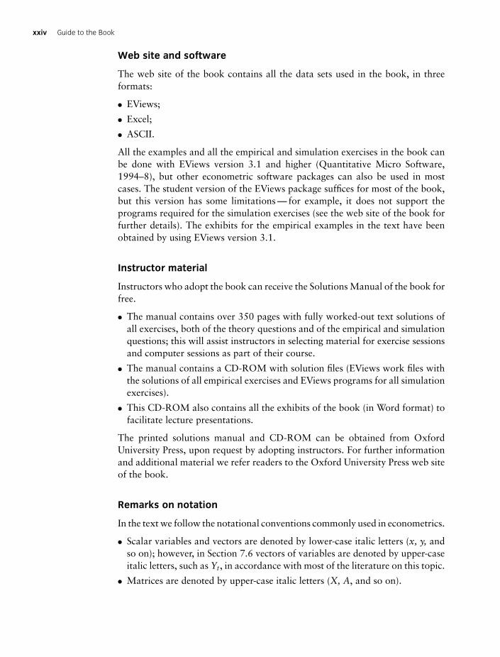
Remarks on notation

In the text we follow the notational conventions commonly used in econometrics.

. Scalar variables and vectors are denoted by lower-case italic letters (x, y, and

so on); however, in Section 7.6 vectors of variables are denoted by upper-case

italic letters, such as Yt, in accordance with most of the literature on this topic.

. Matrices are denoted by upper-case italic letters (X, A, and so on).

Heij / Econometric Methods with Applications in Business and Economics Final Proof 28.2.2004 6:12pm page xxiv

xxiv Guide to the Book

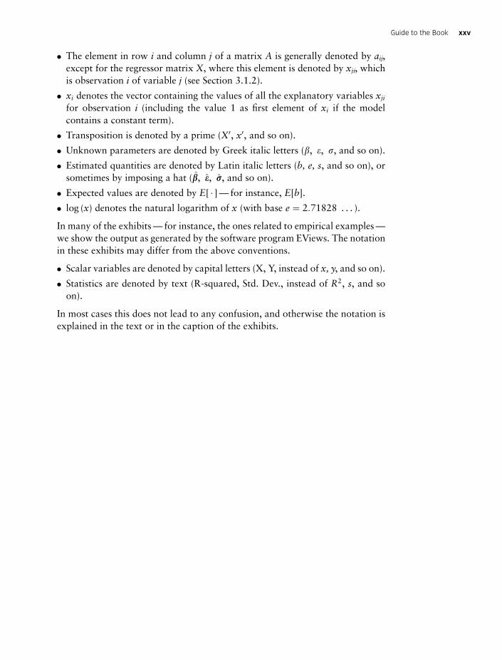
. The element in row i and column j of a matrix A is generally denoted by aij,

except for the regressor matrix X, where this element is denoted by xji, which

is observation i of variable j (see Section 3.1.2).

. xi denotes the vector containing the values of all the explanatory variables xjifor observation i (including the value 1 as first element of xi if the model

contains a constant term).

. Transposition is denoted by a prime (X0, x0, and so on).

. Unknown parameters are denoted by Greek italic letters (b, e, s, and so on).

. Estimated quantities are denoted by Latin italic letters (b, e, s, and so on), or

sometimes by imposing a hat (bb, ee, ss, and so on).

. Expected values are denoted by E[ _ ] — for instance, E[b].

. log (x) denotes the natural logarithm of x (with base e ¼ 2:71828 . . . ).

In many of the exhibits — for instance, the ones related to empirical examples —

we show the output as generated by the software program EViews. The notation

in these exhibits may differ from the above conventions.

. Scalar variables are denoted by capital letters (X, Y, instead of x, y, and so on).

. Statistics are denoted by text (R-squared, Std. Dev., instead of R2, s, and so

on).

In most cases this does not lead to any confusion, and otherwise the notation is

explained in the text or in the caption of the exhibits.

Heij / Econometric Methods with Applications in Business and Economics Final Proof 28.2.2004 6:12pm page xxv

Guide to the Book xxv

Documents

Econometric Methods with Applications in Business and