ECONOMETRIC METHODS AND Study MODELS USED IN THE … · 2019. 8. 12. · using econometric methods, parameters which express interdependence, meaning and intensity of correlation

Network Intelligence Studies Volume V, Issue 9 (1/2017)

67

Constantin ANGHELACHE Bucharest University of Economic Studies, Faculty of Faculty of Cybernetics, Statistics and

Economic Informatics /„Artifex” University of Bucharest, Faculty of Finance and Accounting Madalina Gabriela ANGHEL

„Artifex” University of Bucharest, Faculty of Finance and Accounting, Romania, Bucharest

ECONOMETRIC METHODS AND MODELS USED IN THE ANALYSIS OF

THE FACTORIAL INFLUENCE OF THE GROSS DOMESTIC PRODUCT

GROWTH

Case Study

Keywords Econometric model, Economic growth,

Correlation, Factor of influence,

Parameter

JEL Classification

E17, O11

Abstract

Gross Domestic Product is the most representative synthetic indicator that expresses the evolution of the national economy. This macroeconomic indicator is used in the analysis of the level of the national economy, as well as the dynamic evolution of the national economy. In the forecast studies we rely on GDP evolution. In these situations, we might identify the factors of economic growth, and their influence. On the evolution of GDP have influence some factors: employees, labour productivity, the level of technology, investments and foreign direct investment, imports, exports or net exports, total consumption, and so on. We can analyze the data series and graphical representation. Detailed analysis is performed using econometric methods, parameters which express interdependence, meaning and intensity of correlation. Thus, we estimate the economic developments. The authors studied and proposed some econometric models for the analysis of economic growth/forecast. The novelty is that we adapt some econometric models to macroeconomic analysis.

Network Intelligence Studies

Volume V, Issue 9 (1/2017)

68

INTRODUCTION

In this article the authors sought to establish the

main methods and models that econometrics offers

in view of such an analysis. It is known that gross

domestic product exerts a number of factors

(variables) that we need to analyze in the

perspective of making some decisions. For

example, factorial variables, ie those that can

determine the evolution of gross domestic product,

the most complex indicator of macroeconomic

results, can be used for statistical-mathematical-

econometric methods. Thus, on the basis of each

series of data, relating to one variable or another,

one can see the trend of evolution from time to

time. Of course, the data itself reveals

quantitatively and analyzed in their complexity

gives the qualitative essence to the perspective and

trend of the national economy. Labor productivity

and the number of employees are factors, whether

we rely on the production function or simply

analyze from the point of view of the two factors,

the perspective and the meaning of the influence of

these factorial variables on the resultant one. The

study, can be deepened by calling to the graphical

representation of the data in the series, resulting in

this graphical representation and evolutionary

trend. Moreover, we can use the index method to

establish a series of indices that make sense of the

evolution of gross domestic product from one

period to the next. For example, the average Gross

Domestic Product Growth index compared to the

average labor productivity growth index, compared

to the average change in the number of employees,

all of which give meaning to the analysis.

However, the dynamic or territorial analysis of the

main macroeconomic indicators should be

complemented by econometric analytical methods

to express more clearly the existence of the link,

the meaning of the link, and especially the intensity

of the link. From this point of view, after analyzing

the data series, the parallel data series (here we

refer to the fact that gross domestic product, labor

productivity, number of employees and other

factorial variables can be presented in parallel data

series) give us the nature or function of that link.

For example, for gross domestic product as a

resolvable variable compared to labor productivity

or the number of employees, the provision of

technological means of production, the use of

working time, the contribution of branches to the

growth of gross domestic product, etc., we can

assume hypotheses on the type of function or

econometric model used. In this paper the authors

identified between the gross domestic product as a

resolutive variable and the other all the factorial

variables of influence the existence of a correlation

(links) with the form of the straight line function.

Starting from this, we can consider this linear

model of interdependence between the two or more

variables, on the basis of which we can construct a

simple linear regression function (the link between

two variables only) or the linear multiple link (the

link between a resolutive variable and several

factorial variables). From the mathematical

procedure regression model we arrive at the

determination of a system of equations by solving

the regression parameters. In turn, these regression

parameters are the basic elements by which we can

estimate the evolution of the gross domestic

product in the future forecasting period, or we can

recalculate the levels achieved in the oscillatory

evolution of these indicators by applying the

regression model. The regression function as a

econometric model is often used and in this paper

the authors have proposed as an objective to

establish and solve by the regression function the

correlation (interdependence) between the variables

on the basis of which they carried out a concrete

analysis. In Methodology research and data, based

on the statistical data provided by the National

Institute of Statistics for all these variables, the

regression parameters were calculated, their

analysis and interpretation were made, suggesting

the possibility to make forecasts for the future,

complex or on each variable in part. This study

offer some conclusions and recommendations on

the use of these econometric methods to determine

the factorial influence of variables on the resulting

variable. In fact, the variables are just the statistical

indicators that we consider to be individualized,

based on data or graphical representations or in

correlation using other, more complex, econometric

methods and models.

LITERATURE REVIEW

Alfaro, Chanda, Kalemli-Ozcan and Sayek (2004)

develop on the role of foreign direct investments in

sustaining the economic growth, particularly the

position of local financial markets in this context,

Anghelache and Anghel (2015) study the

correlation between FDI balance and GDP at the

European level, Anghelache, Partachi, Sacală and

Ursache (2016), Anghelache and Manole (2012)

apply econometric techniques in the scope of this

type of analysis. Anghel, Anghelache, Dumitrescu

and Dumitrescu (2016) describe the evolution of

the Gross Domestic Product of Romania by

emphasizing the influence of selected factor

variables, while Anghel, Diaconu and Sacală

(2015) focus on the uses categories in the study of

Romania’s GDP, Dumitrescu, Anghel and

Anghelache (2015) evaluate the role of structural

variables on the GDP evolution. Bardsen Nymagen

and Jansen (2005), Corbore, Durlauf and Hansen

(2006), Anghelache and Anghel (2016), Guijarati

(2005) present the concepts and instruments of

econometrics, together with illustrative case



69

studies. Cicak and Soric (2015) analyse the

correlation between foreign direct investments, for

the case of countries with economies in transition.

Koulakiotis, Lyroudi, Papasyriopoulos (2012)

study the situation of inflation and Gross Domestic

Products in the European economies. Anghelache

and Anghel (2015) describe the usefulness of

statistical-econometric models and methods in the

analysis of the Gross Domestic Product. Céspedes

and Velasco (2012) study the dynamics of

macroeconomic performances under the impact of

major dynamics of prices for commodities.

Anghelache, Soare and Popovici (2015) consider

the influence of the final consumption on the Gross

Domestic Product, while Anghelache, Manole and

Anghel (2015) develop a study based on multiple

regression where the GDP is considered the main

indicator, while final consumption and gross

investments form the influence factors. Büthe and

Milner (2008) consider the application of

international trade agreements as instruments for

increasing the foreign direct investments. An in-

depth analysis of the final consumption is presented

by Anghelache, Manole and Anghel (2015).

Anghelache, Anghel and Sacală (2014),

Anghelache, Anghel, and Popovici (2016) realize

top-level analyses of the Romanian Gross Domestic

Product. Lucas and Moll (2014) approach some

issues on knowledge development. Anghelache and

Anghel (2016) develop on the basics of economic

statistics, their approach aims both the theoretical

framework and practical study. Capinski and

Zastawniak (2003) is a reference work in the field

of financial mathematics. De Michelis and Monfort

(2008) develop on the European cohesion policy, in

relation to regional convergence and the Gross

Domestic Product. Dornbusch, Fischer and Startz

(2007) is a comprehensive reference on

macroeconomic topics. Garín, Lester and Sims

(2016) evaluate the desirable character of targeting

nominal Gross Domestic Product. Guner, Ventura

and Yi (2008) consider the macroeconomic effects

of policies depending on size of companies.

RESEARCH METHODOLOGY AND DATA

In this article, the authors emphasized the analysis

of the Gross Domestic Product series, the Gross

Domestic Product Index, labor productivity, the

Gross Gross Value Index, the census index of the

employed population and the index of the increase

in the number of employees. The data series are

presented in table no. 1.

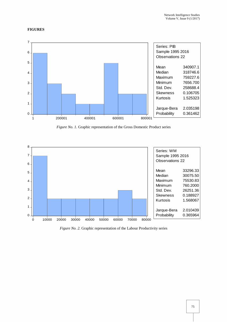
From the study of the data series in Table 1 shown,

both in absolute figures (Gross Domestic Product

and Labor Productivity) and in relative figures

(Gross Domestic Product Indices, gross value

added, employed population and number of

employees) were registered The same

developments. With small oscillations, in absolute

terms, GDP and labor productivity have risen

steadily. The GDP growth index, on the growth

trend in absolute figures, registered significant

leaps until 2008, when the financial crisis started in

Romania. The crisis period was characterized by

temperate growth indices, even a negative trend (-

2.64) in 2009. The same trend was registered by the

gross value added, the employed population and the

number of employees. In conclusion, the simple

study of the databases shows that GDP, in absolute

or relative value, as a resolvable variable, is

influenced by all the other factorial variables. The

graphical representation of all these indicators

(statistically variable) further highlights a

correlative evolutionary trend. In this context, for

the quantification of the existing correlation

between GDP and each of the factorial variables or

between GDP and all other variables, the authors

used simple and multiple linear regression models.

The linear regression functions are of the form:

- linear linear regression:

𝑦𝑖 = 𝑎 + 𝑏𝑥𝑖 + 𝜀

where:

yi = resulting variable;

xi = factorial variable;

a, b = regression parameters;

= residual variable.

- multiple linear regression:

𝑦𝑖 = 𝑎0 + 𝑎1𝑥1 + 𝑎2𝑥2 +⋯+ 𝑎𝑛𝑥𝑛 + 𝜀

where:

yi = resulting variable;

x1, x2 ... xn, = factorial variables;

a0 = regression parameter, free term;

a1, a2 ... an = the regression parameters associated

with each variable;

= residual variable.

By replacing the variables considered in the above-

described regression functions and by solving the

resulting equation systems we obtain the regression

parameters on the basis of which we will deepen

the analysis.

• The correlation between GDP and labor

productivity

The regression model becomes:

PIB = C(1) + C(2)WM + ε, where C(1) și C(2) are the regression parameters.

Estimation of the regression parameters is done by

the least squares method, using the Eviews

software in this regard, the results being presented

in figure no. 4.

The regression model established by estimating the

parameters is:

PIB = 13257,08 + 9,840424 WM +

The regression model is characterized by

significant values of R-squared and Adjusted R-

squared parameters, respectively over 99.7%. This

is the possibility to explain the variation of the

Gross Domestic Product by the labor productivity



70

dynamics, to over 99.7%. The value of parameter

C(2) shows that, with a unit labor productivity

increase, GDP will increase by more than 9.84

units of currency. We consider that the value of the

coefficient C(1), sensitively higher than the

regression coefficient, indicates the presence of

additional influence factors on the dependent

variable.

Next, we can use the same model to calculate the

regression parameters specific to the correlation

between GDP and each resulting variable. Also,

correlation models can be constructed between

variables considered factorial, but only after a

thorough database study and graphical

representation.

• Multiple regression model using

absolute values

In this regression model we used indicators

expressed in absolute figures given in table no. 2

and graphically represented in figure no. 5,

resulting in the estimated parameters in figure no.

6.

The regression model established on the basis of

the estimated parameters is of the form:

GDP = 6396,532 + 6,398910 WM + 0,393516

VAB + 4,275748 POC – 7,876439 EMP +

Analyzing the coefficients of the estimated

regression model, we note that three of the four

factorial variables exert a positive influence on the

Gross Domestic Product. In order of the

significance level of influence, the most important

factor is labor productivity: an increase in a unit of

labor productivity generates a plus of more than

6.39 monetary units of the independent variable.

The increase by one person of the value of the

employed population leads to an increase of the

GDP by over 4.27 lei. The increase in gross added

value leads to a sub-unitary increase of GDP,

respectively to one u.m. We add a plus of 0.39 of

the Gross Domestic Product. Instead, the number of

employees exerts a negative influence on the main

indicator. The high C (1) coefficient indicates the

existence of additional factors that influence GDP

and whose overall impact is positive. The R-

squared and Adjusted R-squared tests associated

with the model attest to model quality and

recommendation for use in later analyzes.

• Multiple regression model using indices

The multiple regression model used is based on the

data of the indicators expressed in relative sizes,

the growth indices presented in table no. 3 and

graphically represented in Fig. 7.

The multiple regression model, introducing the

estimated regression parameters presented in figure

no. 8, is of the form:

IPIB = -1,650543 + 0,524385 IWM + 41,17533

IVAB + 46,02154 IPOC – 84,22157 IEMP +

As the associated indicator (Gross Domestic

Product), the GDP index is influenced by the

indices corresponding to the four macroeconomic

indicators, and this influence explains the IPIB

variation in the proportion of over 98%. The most

significant influence is recorded in the index of

growth of the employed population: the increase by

one percentage point of this indicator leads to a

46% increase in the GDP index. For the gross

added value index, the regression coefficient is

41.17. While the index of the number of employees

exerts a negative influence, characterized by a

coefficient of -84.22, the labor productivity index is

characterized by the lowest positive influence on

the independent variable. It is worth noting the high

and, at the same time, negative value of the free

expression of other factorial variables of IPIB,

whose combined impact is negative.

CONCLUSION

In this article, the authors focused on highlighting

the main statistical, econometric or mathematical

methods or all in one place in analyzing the

evolution of gross domestic product. Of course, this

evolution is presented precisely at each point in

Methodology research and data, allowing those

wishing to deepen the analysis to use the same

methods, the same extension models of the

analysis. The emphasis was put on the use of the

data series method, the graphical representation

method, the evolution index method, or the simple

and multiple linear regression models that they

applied to the study of gross domestic product

evolution over a sufficiently long period of time for

data to have the essence and meaning desired in the

analysis. Interpretation of regression parameters

and then their use highlighted the extent to which

each of the applied factor variables have meaning,

intensity and direction of influence on the gross

domestic product, allowing the researcher or the

manager to choose the optimal variant he wishes to

Use it in the analysis of gross domestic product

development. Of course, the analysis can be

deepened by interpreting the gross domestic

product structure, by resources and utilities, as well

as interpreting the influence of private

consumption, final consumption, or investment on

gross domestic product growth. All those are

elements of possible expansion and development of

the evolution of gross domestic product. Certainly,

other macroeconomic outcome indicators can be

analyzed over a period of time or forecasting using

the same methods. Designed models can be

completed, can be simplified, but they are an



71

accurate and useful statistical and econometric

instrument in macroeconomic analyzes. The

authors consider that the models agreed in this

article are concrete theoretical and practical

examples that highlight the usefulness of using

these methods and econometric models in

macroeconomic analyzes. At each point in

Methodology research and data, the authors also

recorded the mathematical functions that can be

used to perform these analyzes.

REFERENCES

[1] Alfaro, L., Chanda, A., Kalemli-Ozcan, S. &

Sayek, S., (2004). FDI and economic growth:

the role of local financial markets. Journal of

International Economics, 64, 89-112

[2] Anghel, M.G., Anghelache, C., Dumitrescu,

D.V. & Dumitrescu, D. (2016). Analysis of the

correlation between the Gross Domestic

Product and some factorial variable. Romanian

Statistical Review, Supplement, 10, 138-145

[3] Anghel, M.G., Diaconu, A. & Sacală, C.

(2015). Analysis of the evolution of Gross

Domestic Product by categories of users.

Romanian Statistical Review Supplement, 10,

35-42

[4] Anghelache, C. & Anghel, M.G. (2016).

Econometrie generală. Concepte, teorie și

studii de caz. Bucureşti: Editura Artifex


Bazele statisticii economice. Concepte

teoretice şi studii de caz. Bucureşti: Editura

Economică

[6] Anghelache, C., Anghel, M.G. & Popovici, M.

(2016). Analysis of the Gross Domestic

Product Evolution for 2015. Romanian

Statistical Review Supplement, 3, 50-56

[7] Anghelache, C., Partachi, I., Sacală, C. &

Ursache, A. (2016). Using econometric models

in the correlation between the evolution of the

Gross Domestic Product and Foreign Direct

Investments. Romanian Statistical Review,

Supplement, 10, 124-129


Model of Analysis of the Dynamics of the DFI

(DFI) Sold Correlated with the Evolution of

the GDP at European Level. Romanian

Statistical Review Supplement, No. 10, 79-85

[9] Anghelache, C., Soare, D.V. & Popovici, M.

(2015). Analysis of Gross Domestic Product

Evolution under the Influence of the Final

Consumption. Theoretical and Applied

Economics, XXII, No.4 (605), Winter, 45-52

[10] Anghelache, C., Manole, A. & Anghel, M.G.

(2015). Analysis of final consumption and

gross investment influence on GDP – multiple

linear regression model. Theoretical and

Applied Economics, No. 3(604), Autumn, 137-

142

[11] Anghelache, C. & Anghel, M.G. (2015). GDP

Analysis Methods through the Use of

Statistical – Econometric Models.

„Economica” Scientific and Didactic Journal,

nr. 1 (91), Chişinău, Republica Moldova, pp.

124-130


(2015). Analysis of Final Consumption, Gross

Investment, the Changes in Inventories and

Net Exports Influence of GDP Evolution, by

Multiple Regression. International Journal of

Academic Research in Accounting, Finance

and Management Sciences, 5(3), July 2015,

66-70


(2015). Unifactorial Econometric Model -

Connection between the Final Consumption

and the Private Consumption. Asian Academic

Research Journal Of Social Science &

Humanities, 2, (6), November, 212-219

[14] Anghelache, C., Anghel, M.G. & Sacală, C.

(2014). The Gross Domestic Product

Evolution. Romanian Statistical Review -

Supplement, No. 12, pg. 12 – 20

[15] Anghelache, C. & Manole, A. (2012).

Correlation between GDP Direct Investments –

An Econometric Approach.

Metalurgia International, nr.8, 96

[16] Bardsen, G., Nymagen, R. & Jansen, E.

(2005). The Econometrics of Macroeconomic

Modelling, Oxford University Press

[17] Büthe, T. & Milner, H. (2008). The Politics of

Foreign Direct Investment into Developing

Countries: Increasing FDI through

International Trade Agreements?. American

Journal of Political Science, 52(4), October

2008, 741–762

[18] Capinski, M. & Zastawniak, T. (2003).

Mathematics for Finance – An Introduction to

Financial Engineering, Springer-Verlag

London Limited

[19] Céspedes, L.F. & Velasco, A. (2012).

Macroeconomic Performance During

Commodity Price Booms and Busts, IMF

Economic Review, 60, December, 570-599.

NBER Working Paper No 18569 (Cambridge,

Massachusetts, National Bureau of Economic

Research)

[20] Cicak, K. & Soric, P. (2015). The

Interrelationship of FDI and GDP in European

Transition Countries. International Journal of

Management Science and Business

Administration, 1, 4, 41-58

[21] Corbore, D., Durlauf, S. & Hansen, B., (2006).

Econometric Theory and Practice – Frontieres

of Analysis and Applied Research, Cambridge

University Press, United Kingdom



72

[22] De Michelis, N. & Monfort, P. (2008). Some

reflections concerning GDP, regional

convergence and European cohesion policy.

Regional Science Policy & Practice, Volume

(Year): 1 (2008), Issue (Month): 1

(November), 15-22

[23] Dornbusch, R., Fischer, S. & Startz, R. (2007).

Macroeconomie - traducere. Bucureşti:

Editura Economică

[24] Dumitrescu, D., Anghel, M.G. & Anghelache,

C. (2015). Analysis Model of GDP

Dependence on the Structural Variables.

Theoretical and Applied Economics, XXII,

No.4 (605), Winter, 151-158

[25] Garín, J., Lester, R. & Sims, E. (2016). On the

Desirability of Nominal GDP Targeting.

Journal of Economic Dynamics and Control,

Volume 69, August 2016, 21–44

[26] Guijarati, D. (2005). Basic Econometrics, The

McGraw – Hill Companies

[27] Guner, N., Ventura, G. & Yi, X. (2008).

Macroeconomic Implications of Size-

Dependent Policies. Review of Economic

Dynamics, 11 (4), pp. 721–744

[28] Koulakiotis, A., Lyroudi, K. &

Papasyriopoulos, N. (2012). Inflation, GDP

and Causality for European Countries.

International Advances in Economic Research,

18, Issue (1), 53-62

[29] Lucas, R.E. & Moll, B. (2014). Knowledge

Growth and the Allocation of Time, Journal of

Political Economy, 122 (1), 1–51

http://www.sciencedirect.com/science/journal/01651889

http://www.sciencedirect.com/science/journal/01651889/69/supp/C



73

TABLES

In this article, we used the following abbreviations: GDP - Gross Domestic Product (the abbreviation of Gross

Domestic Product in Romanian language is PIB); IGDP - Index of Gross Domestic Product (the abbreviation of

Index of Gross Domestic Product in Romanian language is IPIB); LP - Labour Productivity (the abbreviation of

Labour Productivity in Romanian language is WM); ILP - Index of Labour Productivity (the abbreviation of

Index of Labour Productivity in Romanian language is IWM); GVA - Gross Value Added (the abbreviation of

Gross Value Added in Romanian language is VAB); IGVA - Index of Gross Value Added (the abbreviation of

Index of Gross Value Added in Romanian language is IVAB); POC - Occupied population; IPOC - Index of

Occupied population; EMP - Employees; IEMP - Index of Employees.

Table No.1

Evolution of the main macroeconomic indicators during 1995-2016 period

Year GDP IGDP LP IGVA IPOC IEMP

1995 7656,7 0 760,2 0 0 0

1996 11463,5 49,72 1155,6 1,50173893 0,987991151 0,974578

1997 25689,1 124,09 2643,3 2,20059604 0,962042862 0,916048

1998 37257,9 45,03 3074,4 1,39932077 1,203103181 0,959703

1999 55479,4 48,91 4527,1 1,4811308 0,999981576 0,899088

2000 81275,3 46,5 6752,6 1,47732441 0,99228034 0,997339

2001 118327,2 45,59 9957,5 1,45838189 0,989388763 0,992847

2002 152630 28,99 14301,6 1,29139429 0,898341982 1,000362

2003 198761,1 30,22 18354,6 1,2867562 0,999519527 1,008729

2004 248747,6 25,15 23477,4 1,25617547 0,983394815 0,999507

2005 290488,8 16,78 27541,5 1,15499015 0,984782794 1,029601

2006 347004,3 19,46 32609,5 1,19417067 1,006852124 1,024978

2007 418257,9 20,53 39334,1 1,20600411 1,003654603 1,051502

2008 524388,7 25,37 48958 1,26321212 1,000117461 1,013505

2009 510522,8 -2,64 49120,9 0,98459482 0,98687793 0,932499

2010 533881,1 4,58 52099,5 1,03718532 0,990598291 0,938827

2011 565097,2 5,85 54593,8 1,03941818 0,991928878 1,017348

2012 595367,3 5,36 60413,9 1,05337269 0,951894915 1,025039

2013 637456 7,07 65512,6 1,07487611 0,991220663 1,005014

2014 668143,6 4,81 68469,4 1,05308641 1,007608467 1,020741

2015 712832,3 6,69 73330,9 1,0586477 0,988465013 1,02867

2016 759227,6 4,8 75530,83 1,20838071 0,960236712 1,057596

Note. Data source: National Institute of Statistics, data processed by authors

Table No.2

Evolution of some macroeconomic indicators during 1995-2016 period

Year GDP LP GVA POC EMP

1995 7656,7 760,2 7217,1 9493 6047,678

1996 11463,5 1155,6 10838,2 9379 5893,936

1997 25689,1 2643,3 23850,5 9023 5399,128

1998 37257,9 3074,4 33374,5 10855,6 5181,562

1999 55479,4 4527,1 49432 10855,4 4658,682

2000 81275,3 6752,6 73027,1 10771,6 4646,287

2001 118327,2 9957,5 106501,4 10657,3 4613,051

2002 152630 14301,6 137535,3 9573,9 4614,72

2003 198761,1 18354,6 176974,4 9569,3 4655

2004 248747,6 23477,4 222310,9 9410,4 4652,704

2005 290488,8 27541,5 256766,9 9267,2 4790,431

2006 347004,3 32609,5 306623,5 9330,7 4910,088

2007 418257,9 39334,1 369789,2 9364,8 5162,967

2008 524388,7 48958 467122,2 9365,9 5232,694



74

2009 510522,8 49120,9 459926,1 9243 4879,48

2010 533881,1 52099,5 477028,6 9156,1 4580,989

2011 565097,2 54593,8 495832,2 9082,2 4660,461

2012 595367,3 60413,9 522296,1 8645,3 4777,152

2013 637456 65512,6 561403,6 8569,4 4801,104

2014 668143,6 68469,4 591206,5 8634,6 4900,684

2015 712832,3 73330,9 625879,4 8535 5041,186

2016 759227,6 75530,83 756300,6 8195,62 5331,54


Table No.3

Evolution of indexes for growth of some macroeconomic indicators during 1995-2016 period

Year IGDP IWM IVAB IPOC IEMP

1995 0 0 0 0 0

1996 49,72 52,01 1,501739 0,987991 0,974578

1997 124,09 128,74 2,200596 0,962043 0,916048

1998 45,03 16,31 1,399321 1,203103 0,959703

1999 48,91 47,25 1,481131 0,999982 0,899088

2000 46,5 49,16 1,477324 0,99228 0,997339

2001 45,59 47,46 1,458382 0,989389 0,992847

2002 28,99 43,63 1,291394 0,898342 1,000362

2003 30,22 28,34 1,286756 0,99952 1,008729

2004 25,15 27,91 1,256175 0,983395 0,999507

2005 16,78 17,31 1,15499 0,984783 1,029601

2006 19,46 18,4 1,194171 1,006852 1,024978

2007 20,53 20,62 1,206004 1,003655 1,051502

2008 25,37 24,47 1,263212 1,000117 1,013505

2009 -2,64 0,33 0,984595 0,986878 0,932499

2010 4,58 6,06 1,037185 0,990598 0,938827

2011 5,85 4,79 1,039418 0,991929 1,017348

2012 5,36 10,66 1,053373 0,951895 1,025039

2013 7,07 8,44 1,074876 0,991221 1,005014

2014 4,81 4,51 1,053086 1,007608 1,020741

2015 6,69 7,1 1,058648 0,988465 1,02867

2016 4,8 7,313 1,208381 0,960237 1,057596




75

FIGURES

Figure No. 1. Graphic representation of the Gross Domestic Product series

Figure No. 2. Graphic representation of the Labour Productivity series

0

1

2

3

4

5

6

7

1 200001 400001 600001 800001

Series: PIB

Sample 1995 2016

Observations 22

Mean 340907.1

Median 318746.6

Maximum 759227.6

Minimum 7656.700

Std. Dev. 258688.4

Skewness 0.106705

Kurtosis 1.525323

Jarque-Bera 2.035198

Probability 0.361462

0

1

2

3

4

5

6

7

8

0 10000 20000 30000 40000 50000 60000 70000 80000

Series: WM

Sample 1995 2016

Observations 22

Mean 33296.33

Median 30075.50

Maximum 75530.83

Minimum 760.2000

Std. Dev. 26251.36

Skewness 0.188927

Kurtosis 1.568067

Jarque-Bera 2.010439

Probability 0.365964



76

Figure No. 3. Corelogram Gross Domestic Product / Labour productivity

Figure No. 4. Parameter estimation regression model GDP / Labour productivity

0

100,000

200,000

300,000

400,000

500,000

600,000

700,000

800,000

96 98 00 02 04 06 08 10 12 14 16

PIB WM



77

Figure No. 5. Graphic representation of Gross Domestic Product and factorial variables during 1995-2016

period

Figure No. 6. Parameter estimation regression model GDP_LP_GVA_POC_EMP

0

100000

200000

300000

400000

500000

600000

700000

800000

19

95

19

96

19

97

19

98

19

99

20

00

20

01

20

02

20

03

20

04

20

05

20

06

20

07

20

08

20

09

20

10

20

11

20

12

20

13

20

14

20

15

20

16

PIB WM VAB POC EMP



78

Figure No. 7. Graphic representation of Gross Domestic Product growth indices and other factorial variables

during 1995-2016

Figure No. 8. Parameter estimation regression model IGDP_ILP_IGVA_IPOC_IEMP

-20

0

20

40

60

80

100

120

140

IPIB IWM IVAB IPOC IEMP

Documents

ECONOMETRIC METHODS AND Study MODELS USED IN THE … · 2019. 8. 12. · using econometric methods, parameters which express interdependence, meaning and intensity of correlation