Econometric advice and beta estimation C - Henry... · Econometric advice and beta estimation November 28th, 2008 Associate Professor Ólan T. Henry Department of Economics ... SPAU

Econometric advice and beta estimation

November 28th, 2008

Associate Professor Ólan T. Henry Department of Economics The University of Melbourne Victoria 3010 Australia Tel: + (03) 8344-5312 Fax: + (03) 8344-6899 E-Mail: [email protected] Home page: http://www.economics.unimelb.edu.au/SITE/staffprofile/ohenry.shtml

1

http://www.economics.unimelb.edu.au/SITE/staffprofile/ohenry.shtml

1. The Capital Asset Pricing Model

The Capital Asset Pricing Model, CAPM predicts that the expected return to the ith asset, , is given by ( )iE r

( ) ( )i f i m fE r r E r rβ ⎡ ⎤= + −⎣ ⎦ , (1)

Where fr is the rate of return to the riskless security and [ ][ ]

,i mi

m

Cov r rVar r

β = .

Essentially the CAPM describes the excess expected return to the ith asset, ( )iE r r− f as a risk premium. This risk premium may be written as a fixed price per unit of risk,

( ) [ ]/i m fE r r Var rλ ⎡ ⎤= −⎣ ⎦ m , multiplied by a quantity of risk, [ ],i mCov r r .

( ) [ ],i f i i mE r r Cov r rλ− = , (2) 2. Estimation of the Capital Asset Pricing Model

Using raw returns, estimates of [ ][ ]

,i mi

m

Cov r rVar r

β = may be obtained from the regression

, ,i t i i m t i tr r ,α β ε= + + , (3) Where, the residual is , ,i t i t i i m tr ,rε α β= − + . Assuming that the risk free rate does not vary substantially with time the data may be transformed to excess returns

and estimates of , , , , ,;i t i t f t m t m t f tR r r R r r= − = − , iβ may be obtained from the regression

, ,i t i m t i tR R ,β ε= + (3’)

2.1 Ordinary Least Squares Typically (3) and (3’) are estimated using the method of Ordinary Least Squares, OLS. This approach obtains estimates of the parameters of interest iα and iβ by minimizing the sum of the squared residuals:

(4) ( ) ( 222, , , ,

1 1 1

ˆˆˆT T T

i t i t i t i t i i m tt t t

r r r rε= = =

= − = − −∑ ∑ ∑ ),α β

2.2 Stability of the estimates There are some concerns about the validity of the OLS estimator of iα and iβ in the presence of outliers. In such circumstances the estimates of iα and iβ may vary with time. It is also possible that estimates of 2

iσ , the variance of the residual, ,i tε , may be affected by the presence of outliers.

2

2.2.1 Least Absolute Deviations There are a range of possible approaches that may be followed in order to allow for outliers, the most popular of which is the Least Absolute Deviations, LAD, approach given by

, , , ,1 1 1

T T T

i t i t i t i t i i m tt t t

r r r rε= = =

= − = − −∑ ∑ ∑ %%% ,α β

Here the estimates are obtained by minimizing the absolute value of the residuals. By focusing on minimizing the sum of the absolute values of the residuals rather than the sum of the squared residuals, the effect of the LAD estimator is to reduce the influence of outlying observations. 2.2.2 Recursive Least Squares Recursive estimates of the parameters of interest may be obtained by allowing the sample to vary in a controlled fashion. There are two main approaches to recursive least squares. The first approach employs an expanding window of observations, while the second employs a fixed window that is rolled across the sample. In the case of an expanding window, the first τ observations are used to form the initial estimate of iα and iβ . An additional observation is then added to the estimation window and the resulting τ+1 observations are used to compute the second estimate of the coefficient vector. This process is repeated until all the observation in the sample have been employed yielding T-τ+1 estimates of iα and iβ . These estimates and their associated standard errors may be plotted to detect evidence of time variation in the coefficient vector. Since the sample size is increasing from τ to T the standard error bands will generally tighten as the sample size increases. The moving window estimator employs τ observations from the sample of T observations. The initial estimates of iα and iβ are obtained using the observations 1,2,3,… τ. Subsequent estimates are obtained using observations 2,3,… τ+1 etc up until the final estimates obtained from observations T-τ to T. Again, these estimates and their associated standard errors may be plotted to detect evidence of time variation in the coefficient vector. Since the standard errors are calculated using τ observations the resulting standard error bands will generally be wider than those based on the full set of T observations. 2.3.3 Hansen’s Test for parameter stability Since the recursive and sequential estimates are only visual guides to the stability of the estimates, we also report Hansen's (1992) test for parameter stability.1 This test examines the regression model (3) for evidence of instability in the residual variance, 2

iσ , the intercept,

iα , the slope coefficient iβ , and then a joint test for instability in all three measures. In performing the Hansen test it is not necessary to impose an arbitrary sample splitting, or to

1 Hansen, B.E. (1992) "Parameter Instability in Linear Models", Journal of Policy Modeling, 14 (4), 1992, pp. 517-533.

3

choose forecast intervals. Rather it is necessary to estimate the model of interest a single time using the full sample of data available to the researcher. The null hypothesis of the Hansen (1992) test is that there is no instability in the parameter of interest, while the alternative is that there is instability in the parameter of interest. A joint test of the null hypothesis of no instability in iα , iβ and 2

iσ can be interpreted as a test for parameter stability in the model (3). Rejection of the joint null hypothesis indicates that the model suffers from parameter instability.

0

1

: The paramter (model) of interest is stable: The paramter (model) of interest is not stable

HH

The test has a nonstandard asymptotic distribution which depends upon the number of coefficients being tested for stability. The decision rule is straightforward; in the absence of a significant test statistic, then the investigator may be reasonably confident that either the model has not displayed parameter instability over the sample or that the data is not sufficiently informative to reject this hypothesis. In the presence of a significant test statistic, the investigator may confidently conclude that the model is misspecified and prone to parameter instability. 3. Discrete versus continuously compounded returns Returns may be calculated discretely or continuously. The discrete return over the interval t-1 to t is given by

, , 1,

, 1

i t i t i tdi t

i t

,p p dr

p−

−

− += , (5)

Where ,i tp represents the price of the ith asset at time t, and represents the value of any dividend payment over the interval t-1 to t.

,i td

On the other hand, the continuously compounded return over the interval t-1 to t is given by ( ), , ,ln ( ) /i t i t i t i tr p d p −= + , 1 (6) In the work discussed below, returns, whether discretely or continuously compounded are calculated from accumulation indices, that is, returns include dividends and capital gains and losses. 4. Estimation Results 4.1 Baseline Sample: Firms

Table 1 presents OLS and LAD estimates of β. The consultant was instructed by the

ACCC to examine data over the period January 1st 2002 to 1st September 2008. This sample period was chosen to avoid potential issues associated with the technology bubble. In unreported results, the consultant examined data over the period January 1st 2000 to 1st September 2008. The results are qualitatively unchanged if this additional data is included.

The data on each asset were sourced from Datastream as was the proxy for the market portfolio, in this case the All Ordinaries Index. Where there are less than 348 observations in the sample, the firm began trading after January 1st 2002. The exceptions to this are AGKX

4

(sample end date 31st October 2006) and AAN (sample end date August 17th 2007 and GAS (sample end date November 17th 2006). The AAN and GAS data are price index data sourced from Bloomberg and provided to the consultant by the ACCC. The actual sample dates for each stock are as follows:

SPAU: 16th December 2005 - 1st September 2008 ENVX: 1st January 2002 - 1st September 2008 APAX: 1st January 2002 - 1st September 2008 SKIX: 2nd March 2007 - 1st September 2008 DUEX: 13th August 2004 - 1st September 2008 HDFX: 17th December 2004 - 1st September 2008 AGKX: 1st January 2002 - 31st October 2006 ORGX 1st January 2002 - 1st September 2008 AAN: 1st January 2002 – 17th August 2007 GAS: 1st January 2002 - 17th November 2006 The Datastream identities for each stock and index are provided in the appendix to this

report. For each of the stocks and equity indices considered, discretely and continuously compounded returns to the accumulation indices were calculated.

Given the short sample available for firms such as DUEX, HDFX, SPAU and particularly SKIX, the use of monthly data is unlikely to produce statistically valid inference. Furthermore, taking into account the problems associated with noise in daily data, a sample of weekly data was collected for each firm. Table 1 presents OLS and LAD estimates of the regression , ,i t i i m t i tr r ,α β= + + ε using both continuously and discretely compounded returns

Table 1: Estimates of Equity β Discrete Returns: Weekly

SPAU ENVX APAX SKIX DUEX HDFX AGKX ORGX AAN GAS β 0.2602 0.3353 0.6492 0.4821 0.6028 0.7422 0.4114 0.5929 0.6459 0.3767 s.e 0.1163 0.0717 0.0949 0.1870 0.1131 0.1291 0.0980 0.1170 0.1290 0.1067 β% 0.2287 0.1372 0.5625 0.6493 0.4268 0.3558 0.3009 0.5309 0.4129 0.2808 s.e 0.1169 0.0725 0.0950 0.1880 0.1138 0.1322 0.0983 0.1179 0.1300 0.1072 N 142 348 348 79 212 194 252 348 294 255

Continuous Returns: Weekly SPAU ENVX APAX SKIX DUEX HDFX AGKX ORGX AAN GAS β 0.2614 0.3454 0.6483 0.4931 0.5962 0.7564 0.4120 0.5785 0.6410 0.3725 s.e 0.1160 0.0720 0.0949 0.1881 0.1132 0.1307 0.0973 0.1105 0.1270 0.1046 β% 0.2271 0.1401 0.5607 0.6368 0.4231 0.3734 0.3015 0.5289 0.4073 0.2769 s.e 0.1164 0.0729 0.0951 0.1888 0.1139 0.1336 0.0976 0.1113 0.1279 0.1050 N 142 348 348 79 212 194 252 348 294 255

Table 8 in section 5.1 below compares the estimates of β obtained using data sampled at the daily, weekly and monthly frequencies. This analysis suggests that the estimates of β obtained are broadly comparable across sampling frequencies and concludes that the weekly frequency offers a reasonable trade-off between the noise in daily data and the small sample issues associated with monthly data.

5

It is clear from table 1 that the choice of discrete or continuous compounding does not manifestly affect the magnitude of the estimate obtained using OLS or LAD. Using discretely compounded returns and OLS, the minimum estimated value for β across the 10 securities considered is 0.2602 for SPAU while the maximum estimated value for β was 0.7422 for HDFX. The corresponding minimum and maximum values obtained from the continuously compounded returns were 0.2614 (SPAU) and 0.7564 (HDFX), respectively. However, it is clear that the estimates themselves vary across estimator, which may suggest the presence of outliers or structural instability. Two of the firms in the sample, AGL and Envestra have relatively long corporate histories. The consultant was instructed to examine longer samples for these firms by the ACCC. Extending the sample for Envestra to run over the period August 29th 1997 to September 1st 2008 yielded an OLS estimate of 0.2053 with a standard error of 0.0557.Similarly, extending the sample for AGL to begin on January 1st, 1990 and end of October 31st 2006 OLS estimation yielded β =0.5056 with a standard error of 0.0555. It is important to note that these estimates for AGL were obtained using a variant of the ASX All Ordinaries Index as the proxy for the Market portfolio. This alternate proxy for the market portfolio, AUSTOLD, is a price rather than accumulation index. No accumulation index for the entire sample period 1990 onward was available on Datastream. 4.2 Alternative estimators of the standard errors Table 1b reports OLS estimates of β for the continuously compounded data used in table 1 along with the OLS, White and Newey-West standard errors2.

Table 1b: Estimates of Equity β: Robust standard errors Continuous Returns: Weekly

SPAU ENVX APAX SKIX DUEX HDFX AGKX ORGX AAN GAS β 0.2614 0.3454 0.6483 0.4931 0.5962 0.7564 0.4120 0.5785 0.6410 0.3725

Asy 0.1160 0.0720 0.0949 0.1881 0.1132 0.1307 0.0973 0.1105 0.1270 0.1046 W 0.1404 0.1114 0.1269 0.1746 0.1539 0.1870 0.1216 0.1102 0.1220 0.1053

N-W 0.1638 0.0977 0.1271 0.1324 0.1462 0.1838 0.1372 0.1140 0.1575 0.1151

Adjusting the standard errors for heteroscedasticity using the White estimator would lead to substantially wider confidence intervals for 5 of the 10 stocks considered (SPAU, ENVX, APAX, DUEX and AGKX) but would not qualitatively alter the confidence intervals for the remaining stocks. Using the Newey-West estimator SPAU, ENVX, APAX, DUEX, HDFX, AGKX and AAN would have appreciably wider confidence intervals than those constructed using the OLS standard errors, while the other confidence intervals would be similar to, or in the case of SKIX substantially narrower than, those constructed using the OLS standard errors. While the Newey-West and White adjusted standard errors tend to be larger than the asymptotic standard errors, there are several instances in Table 1b where the degree of disagreement between these robust estimators is negligible (APAX, and ORGX). Typically

2 See the technical appendix for an outline of the various approaches to calculating standard errors

6

the White standard errors tend to be larger than the OLS standard errors but smaller than the Newey-West standard errors. However, given the problems associated with the choice of q in the Newey-West estimator our preference is not to adjust the standard errors for the potential presence of heteroscedasticity using the Newey-West estimator. Were an adjustment to be made, the White estimator would appear to be more appropriate. However, given the lack of clear motivation for any adjustment, and the associated difficulties choosing the appropriate method of adjustment, the unadjusted OLS standard errors will be reported in all subsequent tables

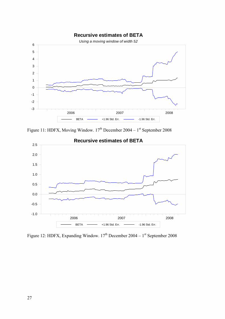
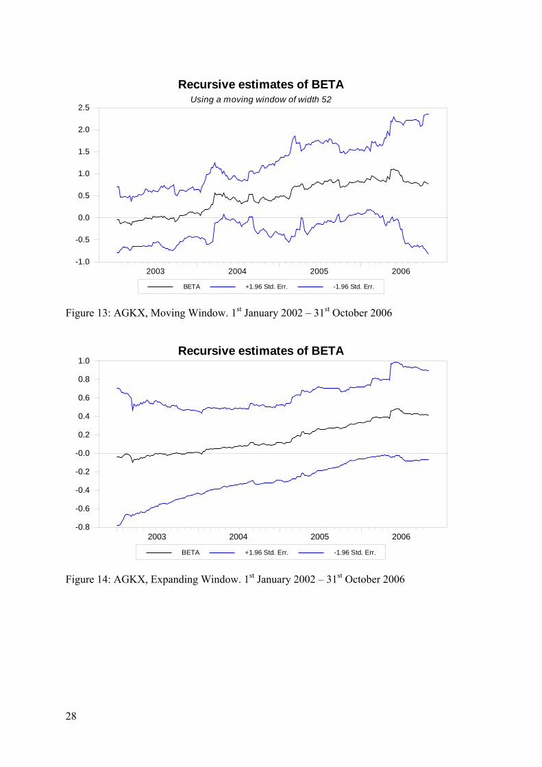
4.3 Structural stability Appendix 1 presents recursive estimates of iβ for each of the i securities using a moving window with a fixed width of 52 observations and an expanding window with initial width of 52 observations. The results for each security are, in general, remarkably similar. First, irrespective of the construction of the recursion, the evidence for each security is consistent. Second, there is only weak visual evidence of time variation in the estimates of iβ across the plots in appendix 1. That is, there are no occasions when the recursive estimates display sudden substantial jumps across all the cases considered. Moreover, there is no systematic evidence of regression to unity. For example, figures 1 and 2 suggest that the β for SPAU lies somewhere between 0.2 and 0.3 (the OLS estimate in Table 1 is 0.2614). Similarly, figures 19 and 20 suggest that the β for GAS lies in the region 0.2 to 0.5 (the OLS estimate in Table 1 is 0.3725. In short, the recursive estimation provides no systematic evidence of parameter instability in the OLS estimates of (3). Table 2 presents marginal significance levels, also referred to as p-values, for the Hansen (1992) test for structural stability applied to OLS estimates of (3) using continuously compounded returns to the accumulation indices.

Table 2: Hansen (1992) Structural Stability Tests

Continuous Returns: Weekly SPAU ENVX APAX SKIX DUEX HDFX AGKX ORGX AAN GAS

Joint 0.02 0.00 0.00 0.27 0.00 0.00 0.01 0.27 0.10 0.14 2σ 0.00 0.00 0.00 0.03 0.00 0.00 0.04 0.12 0.94 0.03

α 1.00 0.05 0.06 1.0 0.92 0.96 0.86 0.35 0.61 0.91 β 0.66 0.72 0.02 0.48 0.40 0.02 0.00 0.33 0.03 0.68

There is some evidence of parameter instability in the estimates across the securities. In 6 out of 10 cases there is evidence against the joint null of no structural instability at the 10% level of confidence or better. In 4 out of 10 cases the joint null is rejected at the 1% level of confidence or better. However in 4 out of 10 cases there is evidence against the null hypothesis of no instability in β at the 10% level of confidence or better. Only one of these rejections is significant at the 1% level of confidence or better. Many of the rejections of the joint null appear to be as a result of instability in 2σ rather than in β. There is no evidence of time variation in α at the 5% level of confidence. In short, where there is evidence of instability in the model, it appears that much of this instability is associated with the variance of the error term, and not with the estimates of the coefficients of the model. 4.4 Baseline Sample: Portfolios

7

As a robustness test, two sets of portfolios were constructed using continuously

compou

iven the concerns about the impact of takeover activity and the quality of the data available

he first portfolio, P1, contains ENVX and APA. Data is available for this portfolio over the

4.4.1 Results for the equally weighted Portfolios

Table 3: Estimates of β: Equal weight portfolios P5

nded returns to the accumulation indices. The first set of portfolios was constructed assuming equal weights, while the second set was based on value weights. As before, we report OLS and LAD estimates of β and in appendix 2 we present recursive estimates of β. Gfor AAN and GAS expressed in section 5.1 below, we exclude these stocks from our portfolio analysis. Moreover, data on these stocks is not available for the full sample period January 1st 2002 – September 1st 2008 as both stocks were delisted prior to the end of the sample. Similarly, AGKX was excluded because of concerns about the impact of corporate restructuring on the price data. Finally, given that the focus of ORGX is retail rather generation we do not consider this stock. Tperiod 1st January 2002 - 1st September 2008. P2 adds DUEX to P1 using data sampled over the period 13th August 2004 - 1st September 2008. Adding HDFX to the constituents of P2 yields the third portfolio sampled over the interval 17th December 2004 - 1st September 2008. The fourth portfolio is estimated over the period 16th December 2005 - 1st September 2008 and contains ENVX, APA, DUEX, HDFX, and SPAU. The fifth portfolio adds SKIX to the constituents of the fourth portfolio. Data over the period 2nd March 2007 - 1st September 2008 is available for the fifth portfolio

P1 P2 P3 P4 Sam le 1 Jan2002 – 13 Aug 2004 – 17 Dec 2004 – 16 Dec 2005 – 2 Mar 2007 – p

1 Sep 2008 1 Sep 2008 1 Sep 2008 1 Sep 2008 1 Sep 2008 Com E E E E Epanies

NVX, APA

NXV,APA,DUEX

NXV,APA,DUEX,HDFX

NXV,APA,DUEX,HDFX

SPAU

NXV,APA, DUEX,HDFX SPAU,SKIX

β 0.4 95 0.5 0.6 91 9 780 2 0.6181 0.6555 s.e 0.0629 0.0731 0.0756 0.0799 0.1075 β% 0.3923 0.5341 0.5511 0.5680 0.6812 s.e 0.0632 0.0733 0.0759 0.0804 0.1078

The point estimates for β obtained using OLS lie in the region 0.4995 - 0.6555. As

iven the possibility of parameter instability in the estimates of β obtained using OLS,

more constituents are added to the portfolios the estimated β increases. This increase in β may be a result of changes in the cross section as more constituents are added to the portfolio or a result of changes in the sample size as less and less time series data is available to the researcher as the cross section increases, or both. The point estimates for β obtained using LAD lie in the region 0.3923 – 0.6812. The LAD estimates increase monotonically as more and more stocks are added to the portfolio and the time series become shorter. Grecursive estimates of the coefficients are reported in appendix 2. The results of this exercise

8

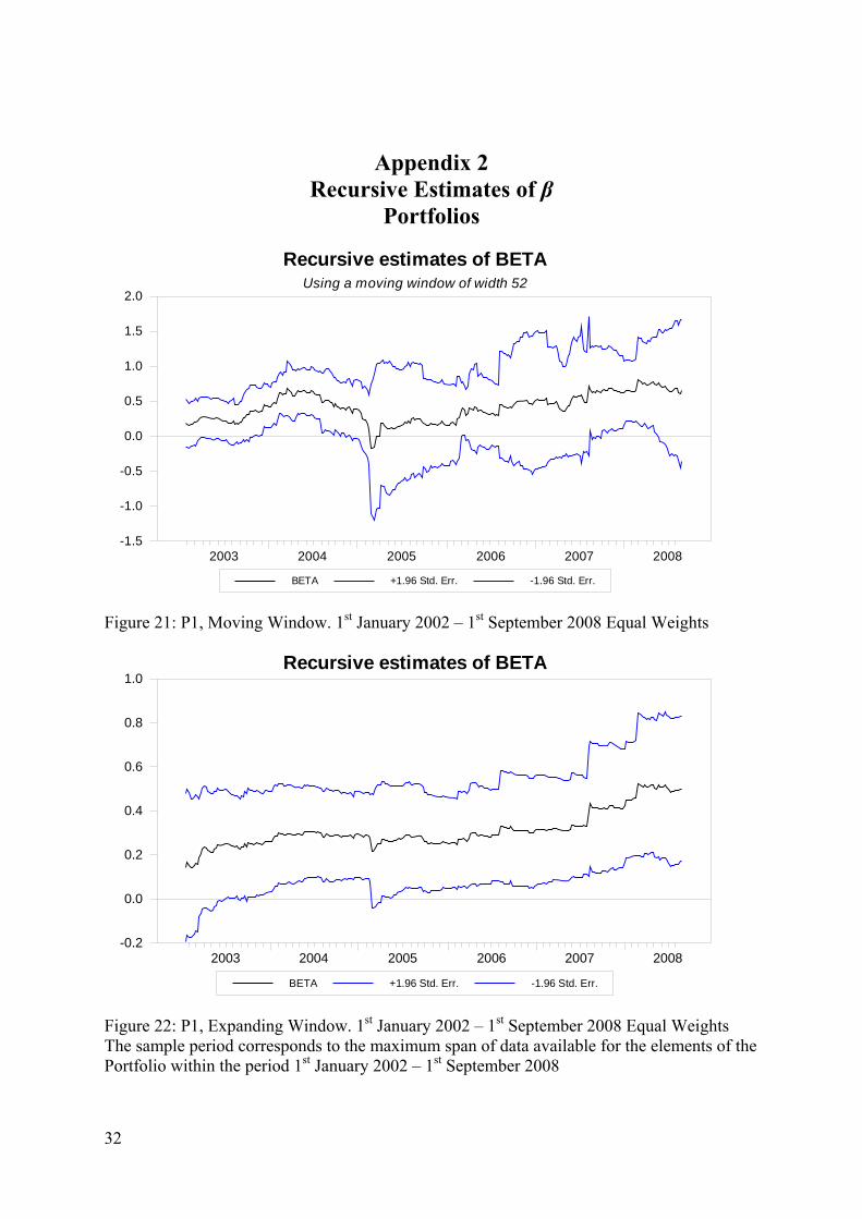
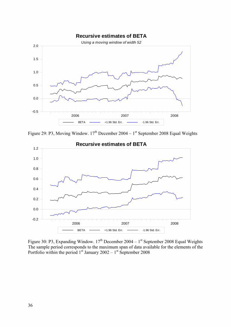
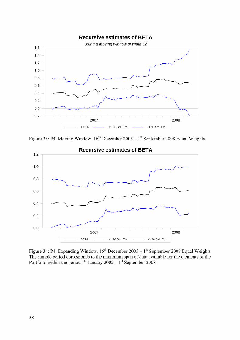
broadly concur with the results reported in appendix 1 for the individual stocks, discussed in section 4.3 above. Appendix 2 presents recursive estimates of iβ for each of the equally weighted portfolios. Results are reported using a moving window with a fixed width of 52 observations and an expanding window with initial width of 52 observations. The results for each portfolio are, in general, remarkably similar. First, irrespective of the construction of the recursion, the evidence for each portfolio is consistent. Second, there is only weak visual evidence of time variation in the estimates of iβ across the plots in appendix 2. That is, there are no occasions when the recursive estimates display sudden substantial jumps across all the cases considered. Moreover, there is no systematic evidence of regression to unity. For example, Figures 21 – 22 display recursive estimates over the period January 1st 2002 to September 1st 2008 for portfolio P1 which contains ENVX and APA. The OLS estimate of β is 0.4995 for P1, which is consistent with the results in Figures 21 and 22 which suggest that, broadly speaking, β lies in the range 0.2 – 0.5. Similarly, figures 37 and 38, which report results for the equal weight portfolio P5 suggest that the recursive estimate β rarely deviates substantially from 0.6 In table 4, the results of the Hansen tests for parameter instability are reported. The table presents marginal significance levels, also referred to as p-values, for the Hansen (1992) test for structural stability applied to OLS estimates of (3) using continuously compounded returns for each portfolio calculated using accumulation indices.

Table 4: Hansen (1992) Structural Stability Tests: Equal weight portfolios P1 P2 P3 P4 P5

Sample

1 Jan2002 – 1 Sep 2008

13 Aug 2004 –1 Sep 2008

17 Dec 2004 –1 Sep 2008

16 Dec 2005 –1 Sep 2008

2 Mar 2007 – 1 Sep 2008

Companies

ENVX, APA

ENXV,APA,DUEX

ENXV,APA,DUEX,HDFX

ENXV,APA,DUEX,HDFX

SPAU

ENXV,APA, DUEX,HDFX SPAU,SKIX

Joint 0.00 0.00 0.00 0.00 0.02 2σ 0.00 0.00 0.00 0.00 0.01

α 0.18 0.79 0.88 0.85 0.76 β 0.06 0.20 0.06 0.41 0.73

In all cases we fail to reject the null hypothesis of no instability in the estimate of β at the 5% level of confidence or better. Similarly there was no evidence of instability in the estimates of α at the 10% level of confidence or better. As with the individual stock return data, rejection of the joint null hypothesis appears to be as a result of instability in the variance of the residual, 2σ rather than as a result of instability in the estimates of α and β across the various portfolios. 4.4.2 Results for the value weighted portfolios Averaging over market capitalization data obtained from obtained from Bloomberg over the period January 1st 2002 to September 1st 2008, value weights were calculated for each stock. These value weights were then employed to construct value weighted portfolios whose constituents match the definitions reported in 4.4.1.

Table 5: Estimates of β: Value weight portfolios

9

P1 P2 P3 P4 P5 Sample

1 Jan2002 – 1 Sep 2008

13 Aug 2004 –1 Sep 2008

17 Dec 2004 –1 Sep 2008

16 Dec 2005 – 1 Sep 2008

2 Mar 2007 – 1 Sep 2008

Companies

ENXV,APA,

ENXV,APA, DUEX

ENXV,APA, DUEX,HDFX

ENXV,APA, DUEX,HDFX

SPAU

ENXV,APA, DUEX,HDFXSPAU,SKIX

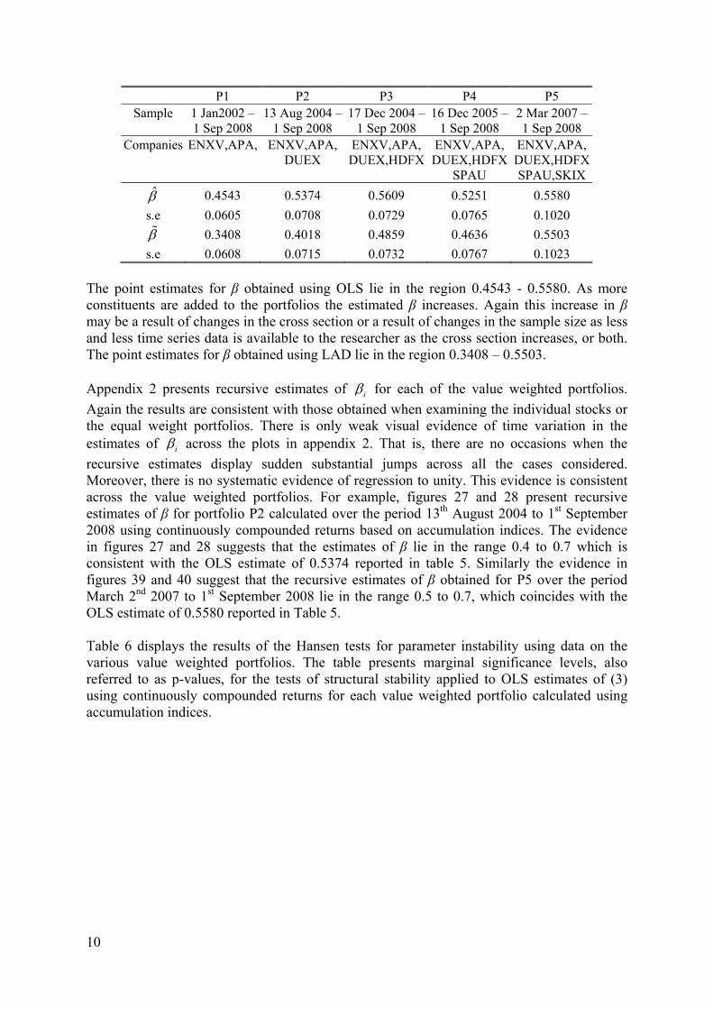
β 0.4543 0.5374 0.5609 0.5251 0.5580 s.e 0.0605 0.0708 0.0729 0.0765 0.1020 β% 0.3408 0.4018 0.4859 0.4636 0.5503 s.e 0.0608 0.0715 0.0732 0.0767 0.1023

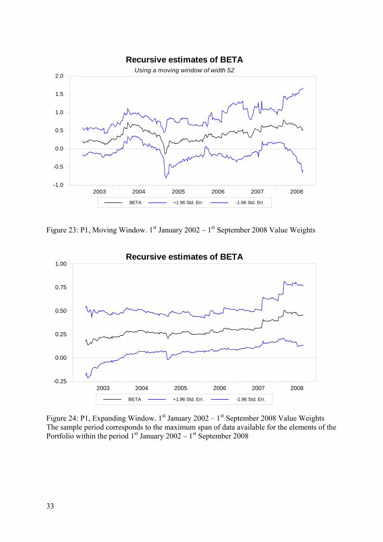
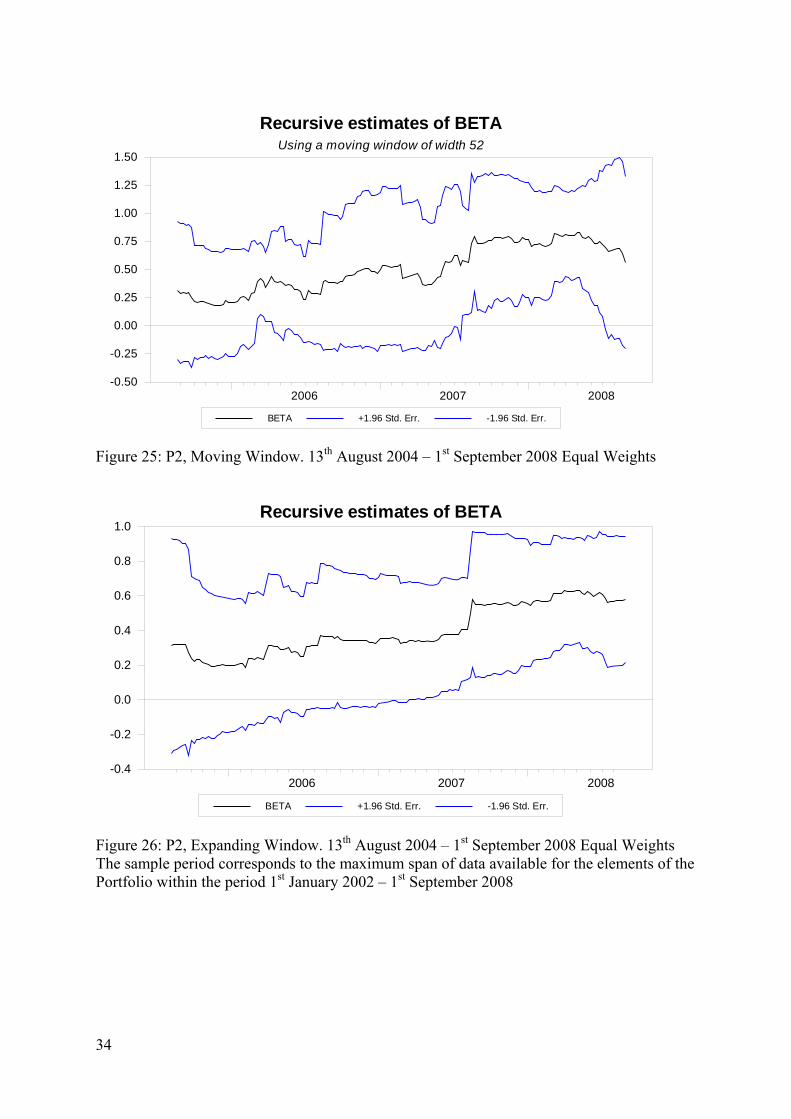
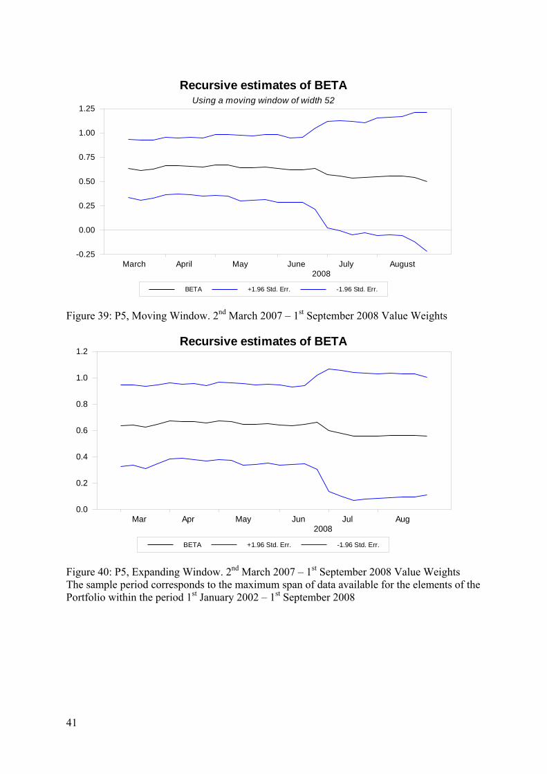
The point estimates for β obtained using OLS lie in the region 0.4543 - 0.5580. As more constituents are added to the portfolios the estimated β increases. Again this increase in β may be a result of changes in the cross section or a result of changes in the sample size as less and less time series data is available to the researcher as the cross section increases, or both. The point estimates for β obtained using LAD lie in the region 0.3408 – 0.5503. Appendix 2 presents recursive estimates of iβ for each of the value weighted portfolios. Again the results are consistent with those obtained when examining the individual stocks or the equal weight portfolios. There is only weak visual evidence of time variation in the estimates of iβ across the plots in appendix 2. That is, there are no occasions when the recursive estimates display sudden substantial jumps across all the cases considered. Moreover, there is no systematic evidence of regression to unity. This evidence is consistent across the value weighted portfolios. For example, figures 27 and 28 present recursive estimates of β for portfolio P2 calculated over the period 13th August 2004 to 1st September 2008 using continuously compounded returns based on accumulation indices. The evidence in figures 27 and 28 suggests that the estimates of β lie in the range 0.4 to 0.7 which is consistent with the OLS estimate of 0.5374 reported in table 5. Similarly the evidence in figures 39 and 40 suggest that the recursive estimates of β obtained for P5 over the period March 2nd 2007 to 1st September 2008 lie in the range 0.5 to 0.7, which coincides with the OLS estimate of 0.5580 reported in Table 5. Table 6 displays the results of the Hansen tests for parameter instability using data on the various value weighted portfolios. The table presents marginal significance levels, also referred to as p-values, for the tests of structural stability applied to OLS estimates of (3) using continuously compounded returns for each value weighted portfolio calculated using accumulation indices.

10

Table 6: Hansen (1992) Structural Stability Tests: Value weight portfolios P1 P2 P3 P4 P5

Sample

1 Jan2002 – 1 Sep 2008

13 Aug 2004 –1 Sep 2008

17 Dec 2004 –1 Sep 2008

16 Dec 2005 –1 Sep 2008

2 Mar 2007 – 1 Sep 2008

Companies

ENVX, APA

ENXV,APA,DUEX

ENXV,APA,DUEX,HDFX

ENXV,APA,DUEX,HDFX

SPAU


Joint 0.00 0.00 0.00 0.00 0.04 2σ 0.00 0.00 0.00 0.00 0.01

α 0.10 0.58 0.60 0.83 0.79 β 0.15 0.34 0.29 0.81 0.46

In all cases we fail to reject the null hypothesis of no instability in the estimate of β at the 5% level of confidence or better. Similarly there was no evidence of instability in the estimates of α at the 5% level of confidence or better. As with the individual stock return data and the equal weight portfolios, rejection of the joint null hypothesis appears to be as a result of instability in the variance of the residual, 2σ , yielding rejections of the joint null of no parameter instability for all portfolios except P5 where the rejection is marginal at the 5% level and is not significant at the 1% level.

4.5 Blume3 and Vasicek4 Adjustments. Blume (1975) inter alia notes that estimated betas that are larger than one tend to be followed by estimated betas that are smaller than one and similarly estimates of beta that are smaller than unity tend to precede estimates that exceed unity. Blume suggest that this tendency for beta to regress towards one requires correction. The Blume estimator for the beta of company i is 0 1

î iβ λ λ β= +B (7)

Here β is an OLS estimate of the beta for company i. Blume estimates the weights as

0 0.33λ = and 1 0.67λ = . Typically, these values for the weights are employed when performing the Blume adjustment. Vasicek (1973) suggests an alternative approach to correct the estimated beta for any tendency to regress towards unity. The Vasicek approach is Bayesian in nature and may be written as

( )ˆ 1Vi i

î iβ β λ λ= − + β (8)

Here β is the sample mean of iβ obtained from a cross section of companies. The weight iλ is calculated as

3 Blume, M. (1975) “Betas and their regression tendencies, Journal of Finance10,(3) 785-795. 4 Vasicek, O. (1973) “A note on using cross-sectional information in Bayesian estimation of security betas”, Journal of Finance 8 (3), 1233-1239.

11

( )

2

2 2 ˆp

ip is

σλ

σ β=

+

Where 2pσ is the sample variance of iβ obtained from a cross section of companies and

( )2is β is the square of the standard error of iβ obtained from the OLS regression used to

obtain iβ . As with the Blume estimator, the weights in the Vasicek estimator sum to one.

Table 7a presents the Blume and Vasicek adjustments to iβ for the continuously compounded weekly stock returns reported in section 4.1, while table 7b presents the adjustments for the equal and value weighted portfolios discussed in section 4.4.

Table 7a: Vasicek and Blume adjustments to β: Stocks Continuously Returns: Weekly

SPAU ENVX APAX SKIX DUEX HDFX AGKX ORGX AAN GAS β 0.2614 0.3454 0.6483 0.4931 0.5962 0.7564 0.4119 0.5785 0.641 0.3725

iβB 0.5051 0.5614 0.7644 0.6604 0.7295 0.8368 0.6060 0.7176 0.7595 0.5796 Viβ 0.3481 0.3736 0.6121 0.5033 0.5673 0.6570 0.4338 0.5598 0.5901 0.4143

The results presented in appendix 1 and 2 suggest that there is little convincing evidence of regression to unity in this data. Therefore, it is difficult to justify the application of the Blume or Vasicek adjustments. The net effect of the adjustments appears to be to increase the magnitude of the estimate of iβ . The results presented in table 7a suggest that the OLS estimates of iβ tend to be smaller than the Vasicek adjusted estimates, which in turn are less than the Blume adjusted estimates.

Table 7b: Vasicek and Blume adjustments to β: Portfolios

P1 P2 P3 P4 P5 Sample

1 Jan2002 – 1 Sep 2008

13 Aug 2004 – 1 Sep 2008

17 Dec 2004 – 1 Sep 2008

16 Dec 2005 – 1 Sep 2008

2 Mar 2007 – 1 Sep 2008

Companies

ENXV,APA,

ENXV,APA, DUEX

ENXV,APA, DUEX,HDFX

ENXV,APA, DUEX,HDFX

SPAU


Fixed Weight Portfolios β 0.4995 0.5780 0.6291 0.6181 0.6555

iβB 0.6647 0.7173 0.7515 0.7441 0.7692 Viβ 0.5495 0.5887 0.6090 0.6041 0.6104

Value Weight Portfolios β 0.4543 0.5374 0.5609 0.5251 0.5580

iβB 0.6344 0.6901 0.7058 0.6818 0.7039 Viβ 0.5037 0.5299 0.5360 0.5266 0.5319

12

The plots of the recursive estimates presented in appendix 2 suggest that there is little evidence of regression to unity in the portfolio β. This in turn suggests that application of the Blume and Vasicek adjustment may be unwarranted. As with the individual returns, the impact of the adjustment is to raise the magnitude of β. Again the OLS estimates of β tend to

e less than the Vasicek adjusted estimates, which in turn are less than the Blume adjusted

ittle vidence of regression towards unity in β. As a consequence there is scant justification for

r correction, which simply inflate the estimate of β without justification.

he results, OLS and LAD estimates of β were obtained using ccumulation index data sampled at the daily, weekly and monthly frequency. The sample

date

08

08

AN: 1st January 2002 – 17th August 2007

he results are reported in table 8 and are broadly consistent with those reported in table 1 for

fter any takeover has been agreed, but prior to delisting hen the time series dynamics of the share price are unusual. In such circumstances daily

een the noisy nature of the daily data and the lack of degrees of freedom in the monthly data. The best compromise would appear to be the use of data sampled at the weekly frequency.

bestimates The Vasicek adjustment has the advantage that the weights are estimated for each cross section of β estimates, unlike the Blume adjustment where the weights estimated by Blume are typically employed despite their lack of relevance to any cross section of β estimates other than those examined by Blume (1975). However, in the current context, there is leemploying eithe 5. Robustness 5.1 Alternative sampling frequencies for the Australian Data In order to ensure robustness of ta

s are as for Table 1, namely

SPAU: 16th December 2005 - 1st September 20ENVX: 1st January 2002 - 1st September 2008 APAX: 1st January 2002 - 1st September 2008 SKIX: 2nd March 2007 - 1st September 2008 DUEX: 13th August 2004 - 1st September 2008HDFX: 17th December 2004 - 1st September 20AGKX: 1st January 2002 - 31st October 2006 ORGX 1st January 2002 - 1st September 2008 AGAS: 1st January 2002 - 17th November 2006

Tthe daily and monthly data and identical for the weekly data. The evidence presented in table 8 suggests that the choice of sampling frequency is largely moot. There is of course one important caveat to this conclusion. In the presence of takeover speculation, there may be frequent halts to trading prior to the actual takeover. Also there may be substantial periods of time awdata may yield unreliable estimates. The bulk of the work in this report uses data sampled at a weekly frequency. Given the sparse nature of the data there are too few monthly observations available for many of the stocks to produce statistically reliable estimates of β. For some of the stocks and portfolios considered in this report there are less than 30 monthly observations meaning that statistical inference using monthly data is unlikely to be reliable. There is a tradeoff betw

13

Table 8: Estimates of β: Alternative sampling frequencies

Continuous Returns: Daily SPAU ENVX APAX SKIX DUEX HDFX AGKX ORGX β 0.4644 0.4869 0.6863 0.6180 0.6252 0.8353 0.4322 0.6541 s.e 0.0471 0.0392 0.0434 0.0696 0.0534 0.0500 0.0414 0.0462 β% 0.3873 0.3737 0.6118 0.5617 0.6571 0.6825 0.4079 0.6891 s.e 0.0472 0.0393 0.0434 0.0697 0.0534 0.0502 0.0414 0.0463 N 708 1736 1736 392 1056 970 1260 1736

Continuous Returns: Weekly SPAU ENVX APAX SKIX DUEX HDFX AGKX ORGX β 0.2614 0.3454 0.6483 0.4931 0.5962 0.7564 0.4120 0.5785 s.e 0.1160 0.0720 0.0949 0.1881 0.1132 0.1307 0.0973 0.1105 β% 0.2271 0.1401 0.5607 0.6368 0.4231 0.3734 0.3015 0.5289 s.e 0.1164 0.0729 0.0951 0.1888 0.1139 0.1336 0.0976 0.1113 N 142 348 348 79 212 194 252 348

Continuous Returns: Monthly SPAU ENVX APAX SKIX DUEX HDFX AGKX ORGX β 0.3388 0.4038 0.5828 0.6934 0.6849 0.6339 0.2463 0.4287 s.e 0.1558 0.1353 0.1781 0.1760 0.2023 0.2258 0.1595 0.2266 β% 0.1728 0.2088 0.6605 0.5153 0.3175 0.4893 0.1051 0.3003 s.e 0.1684 0.1372 0.1783 0.1816 0.2098 0.2273 0.1618 0.2280 N 32 80 80 18 48 44 57 80

We do not report estimates for Alinta and Gasnet in table 8. Alinta was delisted in October 2007 but had been a source of buyout speculation from at least January 2007 GasNet was delisted in November 2006, but again had been subject to takeover speculation as early as Jun 2006. The estimates of β for these stocks are not robust to inclusion of data close to the takeover. Moreover as the sampling frequency increases the estimates approach zero. For example the OLS estimate of β for GasNet obtained using data sampled at a weekly frequency over the period 1st January 2002 to 14th November 2006 is 0.3522. If daily data is employed this estimate falls to 0.031. Similar effects are noticed with Alinta. Using weekly data the OLS estimate of β is 0.6410, which falls to 0.0662 when daily data is employed. As a consequence, any inference about the undiversifiable risk of these stocks should be treated with some caution unless the takeover period is explicitly excluded. As any choice of the reduced sample period is entirely arbitrary, we do not explore this matter any further 5.2 Thin Trading Thin trading can create issues with the magnitude of the estimate of β. In effect, if the stock does not trade regularly, the OLS estimate of β tends to be biased towards zero. In the

14

literature there are 2 popular approaches to adjusting for thin trading. The Scholes-Williams5 approach constructs a measure of β as:

( )

( )

1 1

1

ˆ ˆ ˆ

ˆ1 2i i iSW

im

β β ββ

ρ

− ++ +=

+ (7)

Where 1îβ− is the estimated slope when ri,t is regressed on rm,t-1, ˆ

iβ is the estimated slope

when ri,t is regressed on rm,t, 1îβ+ is the estimated slope when ri,t is regressed on rm,t+1, and

1 ˆmρ is the estimated first order serial correlation coefficient for rm,,t . While the Scholes-

Williams measure of β has the advantage of simplicity, it relies on estimates of 1iβ− and 1

iβ+

that are obtained from regressions whose theoretical foundation suggests a potential for omitted variable bias. Moreover, calculation of a standard error for (7) is a non-trivial task. The Dimson6 approach involves estimation of the regression , 1 , 1 , 1 , 1i t i i m t i m t i m t i tr r r r ,α β β β− − + += + + + + ε , (8)

The Dimson estimate of β, Diβ is obtained from sum of the coefficients of the independent

variables in equation (8). If the CAPM is the correct model of equilibrium returns then the lag and lead of rm,,t are irrelevant variables. Inclusion of these variables may lead to inefficient estimates of β, but there is little danger of the potential for bias underlying SW

iβ . Additionally, calculation of a standard error for D

iβ is straightforward.

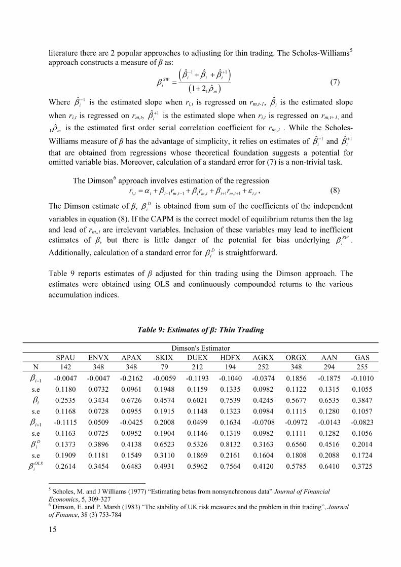
Table 9 reports estimates of β adjusted for thin trading using the Dimson approach. The estimates were obtained using OLS and continuously compounded returns to the various accumulation indices.

Table 9: Estimates of β: Thin Trading

Dimson's Estimator SPAU ENVX APAX SKIX DUEX HDFX AGKX ORGX AAN GAS

N 142 348 348 79 212 194 252 348 294 255

1iβ − -0.0047 -0.0047 -0.2162 -0.0059 -0.1193 -0.1040 -0.0374 0.1856 -0.1875 -0.1010 s.e 0.1180 0.0732 0.0961 0.1948 0.1159 0.1335 0.0982 0.1122 0.1315 0.1055

iβ 0.2535 0.3434 0.6726 0.4574 0.6021 0.7539 0.4245 0.5677 0.6535 0.3847 s.e 0.1168 0.0728 0.0955 0.1915 0.1148 0.1323 0.0984 0.1115 0.1280 0.1057

1iβ + -0.1115 0.0509 -0.0425 0.2008 0.0499 0.1634 -0.0708 -0.0972 -0.0143 -0.0823 s.e 0.1163 0.0725 0.0952 0.1904 0.1146 0.1319 0.0982 0.1111 0.1282 0.1056

Diβ 0.1373 0.3896 0.4138 0.6523 0.5326 0.8132 0.3163 0.6560 0.4516 0.2014

s.e 0.1909 0.1181 0.1549 0.3110 0.1869 0.2161 0.1604 0.1808 0.2088 0.1724 OLSiβ 0.2614 0.3454 0.6483 0.4931 0.5962 0.7564 0.4120 0.5785 0.6410 0.3725

5 Scholes, M. and J Williams (1977) “Estimating betas from nonsynchronous data” Journal of Financial Economics, 5, 309-327 6 Dimson, E. and P. Marsh (1983) “The stability of UK risk measures and the problem in thin trading”, Journal of Finance, 38 (3) 753-784

15

s.e 0.1160 0.0720 0.0949 0.1881 0.1132 0.1307 0.0973 0.1105 0.1270 0.1046 t-ratio -0.6506 0.3743 -1.5139 0.6855 -0.3403 0.2628 -0.5966 0.4287 -0.9071 -0.9925

There is little evidence of systematic distortion caused by thin trading. Comparing the estimates obtained from the Dimson approach with the OLS estimates, D

iβ < OLSiβ in most,

but not all cases. However, the coefficients associated with the lagged and leads of the return to the market portfolio are rarely significant. Moreover, tests of the null hypothesis

D0 : OLS

iH i β β= are uniformly insignificant. The t-ratio test of the null hypothesis never exceeds 2 in absolute value suggesting that there is no statistically significant difference between D

iand . OLSiβ β

On the basis of the evidence in Table 9 there is no support for any adjustment of β to correct for thin trading. 5.3 UK Data Daily, weekly and monthly samples of a comparable UK stock, NG, and proxy for the market portfolio FTSE100 over the period 1st January 2002 - 1st September 2008 were collected and used to obtain estimates of β using the OLS and LAD estimators. The data were used to create continuously compounded returns to the various accumulation indices and the results are reported in Table 10.

Table 10: Estimates of β for UK stocks: Alternative sampling frequencies Daily Weekly Monthly

N 1739 348 80 β 0.5439 0.4530 0.5561 s.e 0.0224 0.0597 0.1282 β% 0.5334 0.4715 0.6301 s.e 0.0224 0.0600 0.1293

Table 10 suggests that the choice of sampling frequency is moot when estimating β for NG, subject to the potential issues with takeovers affecting the quality of daily prices.

5.4 US Data

Daily, weekly and monthly samples of comparable stocks and the Standard and Poor’s Composite Index for the USA over the period 1st January 2002 - 1st September 2008 were collected and used to obtain estimates of β using the OLS and LAD estimators. The list of companies examined in this section was provided to the consultant by the ACC. The results for continuously compounded accumulation returns are reported in Table 11.

16

Table 11: Estimates of β for US stocks: Alternative sampling frequencies US Stocks: Daily

CHG CNP EAS NI NJ NST NU SRP UIL POM β 0.6776 0.6802 0.5039 0.6986 0.6678 0.5298 0.5966 0.9614 0.6423 0.6267 s.e 0.0251 0.0689 0.0282 0.0267 0.0226 0.0208 0.0259 0.0589 0.0310 0.0243 β% 0.6468 0.7506 0.5183 0.6676 0.7122 0.4722 0.5629 0.8899 0.6160 0.6304 s.e 0.0251 0.0690 0.0282 0.0267 0.0226 0.0208 0.0259 0.05589 0.0310 0.0243 N 1736 1736 1736 1736 1736 1736 1736 1736 1736 1736

US Stocks: Weekly CHG CNP EAS NI NJ NST NU SRP UIL POM β 0.7054 0.6142 0.4801 0.6802 0.9593 0.5322 0.5966 0.9684 0.7191 0.7447 s.e 0.0644 0.1594 0.0626 0.0644 0.1204 0.0521 0.0667 0.1621 0.0777 0.0641 β% 0.6939 0.9231 0.4371 0.7991 0.9679 0.4633 0.6153 0.8577 0.7567 0.8039 s.e 0.0645 0.1603 0.0626 0.0648 0.1204 0.0523 0.0666 0.1624 0.0778 0.0643 N 347 347 347 347 347 347 347 347 347 347

US Stocks: Monthly CHG CNP EAS NI NJ NST NU SRP UIL POM β 0.4402 1.4706 0.3657 0.6143 0.8806 0.4658 0.5209 1.7964 1.1663 0.6091 s.e 0.1481 0.3395 0.1503 0.1593 0.2448 0.1285 0.1694 0.4045 0.2097 0.1568 β% 0.4717 1.0207 0.0636 0.6725 0.6841 0.5674 0.4798 1.3746 1.054 0.5839 s.e 0.4183 0.3443 0.1544 0.1604 0.2463 0.129 0.1696 0.4074 0.2163 0.1571 N 80 80 80 80 80 80 80 80 80 80

The evidence in table 11 suggests that the choice of sampling frequency is not important when estimating β for the sample of US stocks. The caveat about the impact of takeover activity on share price dynamics would suggest that the daily frequency may be less useful than weekly and/or monthly data. 6. Delevered/Relevered estimates of β for weekly frequency

Let Aβ and Eβ represent the asset and equity β, respectively. Assuming a debt β of zero, the delivering/relevering equation is

A EEV

β β=

Here E/V is the proportion of equity in the firm’s capital structure. The average gearing level is calculated for the sample period used obtain estimates of the firm or portfolio β using data obtained from Bloomberg. The level of gearing is usually defined as the book value of debt divided by the value of the firm as represented by the sum of the market value of equity and the book value of debt. Define the average level of gearing as G , then

DG

D E=

+

Where D is the book value of net debt and E is the market value of equity. The resulting corporate gearing assumptions are reported in table 12

17

Table 12: Corporate Gearing Assumptions Company Gearing Source

SPAU 58.76% Bloomberg ENVX 71.14% Bloomberg APAX 55.04% Bloomberg SKIX 52.51% Bloomberg DUEX 76.20% Bloomberg HDFX 46.52% Bloomberg AGKX 27.76% Bloomberg ORGX 26.38% Bloomberg AAN 65.64% Bloomberg GAS 41.79% Bloomberg

Portfolio P1 63.09% Bloomberg P2 67.62% Bloomberg P3 62.38% Bloomberg P4 61.90% Bloomberg P5 60.31% Bloomberg

It is possible to show that the appropriate re-levering factor that should be applied to the raw beta estimates is:

11 0.60

Gω −=

−

If it is assumed that ω is constant and that the G is independent of β then, the re-levered β, ˆ

rβ has a mean of ˆωβ and a variance of 2 2β

ω σ . The results of the delevering/relevering

process for individual stocks are reported in table 13

Table 13: Delevered/Relevered estimates of β for weekly frequency: Stocks SPAU ENVX APAX SKIX DUEX HDFX AGKX ORGX AAN GAS

N 142 348 348 79 212 194 252 348 294 255 β 0.2695 0.2492 0.7287 0.5854 0.3547 1.0113 0.7441 1.0647 0.9328 0.3200 s.e 0.1196 0.0519 0.1067 0.2233 0.0674 0.1747 0.1996 0.2034 0.1848 0.0899 β% 0.2341 0.1011 0.6302 0.7560 0.2517 0.4992 0.5445 0.9734 0.5927 0.2379 s.e 0.1200 0.0570 0.1069 0.2242 0.0678 0.1786 0.1763 0.2048 0.1861 0.09020 ω 1.031 0.7215 1.124 1.1873 0.595 1.337 1.806 1.8405 1.4553 0.8590

Considering the delevered/relevered β estimates for the equities the OLS point estimates range from 0.2492 to 1.0647. The corresponding delevered LAD estimates range from 0.1011 to 0.9734. Similarly, the portfolio betas were delevered/relevered. The results are reported in table 14

18

Table 14: Delevered/Relevered estimates of β for weekly frequency: Portfolios Equal Weighted Portfolios

P1 P2 P3 P4 P5 β 0.4609 0.46782 0.5916 0.5887 0.6243 s.e 0.0580 0.05917 0.0711 0.0761 0.1024 β% 0.3620 0.43229 0.5183 0.5410 0.6488 s.e 0.0583 0.05933 0.0714 0.0766 0.1027

Value Weighted Portfolios P1 P2 P3 P4 P5 β 0.4192 0.4350 0.5276 0.5001 0.5314 s.e 0.0558 0.0573 0.0686 0.0729 0.0971 β% 0.3145 0.3252 0.4570 0.4415 0.5241 s.e 0.0561 0.0579 0.0688 0.0730 0.0974

The delevered/relevered OLS estimates of β for the equal weight portfolios range from 0.4609 to 0.6243, while the corresponding estimates for the value weighted portfolios range from 0.4192 to 0.5314. 7. Other Influences on Estimated Betas

Under paragraph 29 of the contract the ACC requested that, where possible, the consultant should quantify the influence of the following factors on the empirical beta estimates:

1. The regulated asset’s place in supply stream (i.e. transmission or distribution);

2. The regulated assets industry (i.e. electricity, gas); and

3. The form of regulatory revenue control (i.e. revenue cap, average revenue cap, weighted average price cap, hybrid).

Given the paucity of the data available it is very difficult to make any meaningful contribution on any of these issues. Ideally if a larger sample of companies were available it would be possible to split this sample into transmission and distribution subsamples and search for systematic biases within the subsamples. However, given that there are only 10 stocks in the sample any variation in beta across sub-samples cannot be reliably detected. Similar comments apply to the industry and form of regulatory control. Even were the data to be pooled to include the overseas firms there is insufficient data in the cross section to address these issues.

8. Summary of advice The following is a brief set of conclusions that have drawn from working with the data described in this document. 8.1 Sampling Frequency A reasonable compromise is to sample the data at a weekly frequency. Given the sparse nature of the data there are too few monthly observations available for many of the

19

stocks to produce statistically reliable estimates of β. For some of the stocks and portfolios considered in this report there are less than 30 monthly observations meaning that statistical inference is unlikely to be reliable. There is a tradeoff between the noisy nature of the daily data and the lack of degrees of freedom in the monthly data. The best compromise would appear to be the use of data sampled at the weekly frequency. 8.2 Construction of Returns Given the results presented above the compounding method does not appear to be an issue. While it is usual to employ continuously compounded returns there is no evidence that β estimates obtained from discretely compounded data are manifestly different. 8.3 Parameter Instability With one important exception, there is no overwhelming issue with instability. It is the case that the OLS and LAD estimates of β differ. However as the estimators are maximizing very different functions, this difference is somewhat unsurprising. Neither of the recursive least squares estimators appears to demonstrate convincing evidence of parameter instability. It is important to note that these estimators are not sufficient in the sense that they do not employ all available information. The use of the Hansen (1992) test for parameter instability produces systematic evidence of instability in the regression models. Where this instability is detected it is almost uniformly due to a change in the error variance in the regression model. There is no evidence of parameter instability associated with the coefficients of the regression models themselves. An exception occurs in the cases of GasNet and Alinta where the estimated betas approach zero as the sampling frequency increases. This appears to be related to the effects of takeover speculation and trading halts prior to the delisting of these stocks. The exclusion of such periods from the sample is very important, but is also arbitrary and depends entirely on the researcher. In short, any estimates of the undiversifiable risk of GasNet and Alinta should be treated with some caution. 8.5 Standard Errors There is evidence of structural instability in the variance of the errors in the estimated model. If there is instability in 2σ it should be possible to date this instability and adjust the model appropriately. Dating this instability and appropriate adjustment are beyond the scope of this report. However, both the White (1980) and Newey-West (1987) estimators correct for heteroscedasticity of unknown form. If the instability can dated a simple correction for heteroscedasticity of a known form can be made. It is not clear what the implications of this instability are for the performance of the White (1980) and Newey-West (1987) approaches to calculating standard errors. Given the difficulties associated with choosing the optimal lag length in the non-parametric estimator of the long run variance, the Newey-West approach appears potentially most fragile. While the confidence intervals obtained using the White and Newey-West corrections can differ from than those obtained using the OLS standard errors, there is no evidence of systematic bias in the standard errors.

20

8.6 Alternative data Re-estimation of the various regression models using US and UK data does not alter the conclusions one would draw about the magnitude of the point estimates β. Similarly delevering does not lead to a revision of the conclusions about the magnitude of β. Rather it is the case that the balance of the evidence points towards the point estimate of β lying in the range 0.4 to 0.7.

21

Appendix 1 Recursive Estimates of β

Individual Stocks

Recursive estimates of BETAUsing a moving window of width 52

BETA +1.96 Std. Err. -1.96 Std. Err.

2007 2008-1.5

-1.0

-0.5

0.0

0.5

1.0

1.5

2.0

2.5

Figure 1: SPAU, Moving Window. 16th December 2005 – 1st September 2008

Recursive estimates of BETA


2007 2008-0.6

-0.4

-0.2

0.0

0.2

0.4

0.6

0.8

1.0

1.2

Figure 2: SPAU, Expanding Window. 16th December 2005 – 1st September 2008

22



2003 2004 2005 2006 2007 2008-2.0

-1.5

-1.0

-0.5

0.0

0.5

1.0

1.5

2.0

2.5

Figure 3: EVX, Moving Window. 1st January 2002 – 1st September 2008



2003 2004 2005 2006 2007 2008-0.6

-0.4

-0.2

0.0

0.2

0.4

0.6

0.8

1.0

Figure 4: EVX, Expanding Window. 1st January 2002 – 1st September 2008

23



2003 2004 2005 2006 2007 2008-4

-3

-2

-1

0

1

2

3

4

Figure 5: APAX, Moving Window. 1st January 2002 – 1st September 2008



2003 2004 2005 2006 2007 2008-0.75

-0.50

-0.25

0.00

0.25

0.50

0.75

1.00

1.25

1.50

Figure 6: APAX, Expanding Window. 1st January 2002 – 1st September 2008

24



Mar Apr May Jun Jul Aug2008

-2

-1

0

1

2

3

Figure 7: SKIX, Moving Window. 2nd March 2007 – 1st September 2008




-1.5

-1.0

-0.5

0.0

0.5

1.0

1.5

2.0

2.5

Figure 8: SKIX, Expanding Window. 2nd March 2007 – 1st September 2008

25



2006 2007 2008-2

-1

0

1

2

3

Figure 9: DUEX, Fixed Window. 13th August 2004 – 1st September 2008



2006 2007 2008-1.0

-0.5

0.0

0.5

1.0

1.5

2.0

Figure 10: DUEX, Expanding Window. 13th August 2004 – 1st September 2008

26



2006 2007 2008-3

-2

-1

0

1

2

3

4

5

6

Figure 11: HDFX, Moving Window. 17th December 2004 – 1st September 2008



2006 2007 2008-1.0

-0.5

0.0

0.5

1.0

1.5

2.0

2.5

Figure 12: HDFX, Expanding Window. 17th December 2004 – 1st September 2008

27



2003 2004 2005 2006-1.0

-0.5

0.0

0.5

1.0

1.5

2.0

2.5

Figure 13: AGKX, Moving Window. 1st January 2002 – 31st October 2006



2003 2004 2005 2006-0.8

-0.6

-0.4

-0.2

-0.0

0.2

0.4

0.6

0.8

1.0

Figure 14: AGKX, Expanding Window. 1st January 2002 – 31st October 2006

28



2003 2004 2005 2006 2007 2008-3

-2

-1

0

1

2

3

4

Figure 15: ORGX, Moving Window. 1st January 2002 – 1st September 2008



2003 2004 2005 2006 2007 2008-1.5

-1.0

-0.5

0.0

0.5

1.0

1.5

2.0

2.5

Figure 16: ORGX, Expanding Window. 1st January 2002 – 1st September 2008

29



2003 2004 2005 2006 2007-3

-2

-1

0

1

2

3

4

5

Figure 17: AAN, Moving Window. 1st January 2002 – 17th August 2007



2003 2004 2005 2006 2007-1.0

-0.5

0.0

0.5

1.0

1.5

2.0

Figure 18: AAN, Expanding Window. 1st January 2002 – 17th August 2007 Data after 17th August 2007 is not available due to the delisting of AAN

30



2003 2004 2005 2006-3

-2

-1

0

1

2

3

Figure 19: GAS, Moving Window. 1st January 2002 – 17th November 2006



2003 2004 2005 2006-0.25

0.00

0.25

0.50

0.75

1.00

Figure 20: GAS, Expanding Window. 1st January 2002 – 17th November 2006 Data after 17th August 2007 is not available due to the delisting of GAS

31

Appendix 2 Recursive Estimates of β

Portfolios



2003 2004 2005 2006 2007 2008-1.5

-1.0

-0.5

0.0

0.5

1.0

1.5

2.0

Figure 21: P1, Moving Window. 1st January 2002 – 1st September 2008 Equal Weights



2003 2004 2005 2006 2007 2008-0.2

0.0

0.2

0.4

0.6

0.8

1.0

Figure 22: P1, Expanding Window. 1st January 2002 – 1st September 2008 Equal Weights The sample period corresponds to the maximum span of data available for the elements of the Portfolio within the period 1st January 2002 – 1st September 2008

32



2003 2004 2005 2006 2007 2008-1.0

-0.5

0.0

0.5

1.0

1.5

2.0

Figure 23: P1, Moving Window. 1st January 2002 – 1st September 2008 Value Weights



2003 2004 2005 2006 2007 2008-0.25

0.00

0.25

0.50

0.75

1.00

Figure 24: P1, Expanding Window. 1st January 2002 – 1st September 2008 Value Weights The sample period corresponds to the maximum span of data available for the elements of the Portfolio within the period 1st January 2002 – 1st September 2008

33



2006 2007 2008-0.50

-0.25

0.00

0.25

0.50

0.75

1.00

1.25

1.50

Figure 25: P2, Moving Window. 13th August 2004 – 1st September 2008 Equal Weights



2006 2007 2008-0.4

-0.2

0.0

0.2

0.4

0.6

0.8

1.0

Figure 26: P2, Expanding Window. 13th August 2004 – 1st September 2008 Equal Weights The sample period corresponds to the maximum span of data available for the elements of the Portfolio within the period 1st January 2002 – 1st September 2008

34



2006 2007 2008-0.50

-0.25

0.00

0.25

0.50

0.75

1.00

1.25

1.50

Figure 27: P2, Moving Window. 13th August 2004 – 1st September 2008 Value Weights



2006 2007 2008-0.2

0.0

0.2

0.4

0.6

0.8

1.0

Figure 28: P2, Expanding Window. 13th August 2004 – 1st September 2008 Value Weights The sample period corresponds to the maximum span of data available for the elements of the Portfolio within the period 1st January 2002 – 1st September 2008

35



2006 2007 2008-0.5

0.0

0.5

1.0

1.5

2.0

Figure 29: P3, Moving Window. 17th December 2004 – 1st September 2008 Equal Weights



2006 2007 2008-0.2

0.0

0.2

0.4

0.6

0.8

1.0

1.2

Figure 30: P3, Expanding Window. 17th December 2004 – 1st September 2008 Equal Weights The sample period corresponds to the maximum span of data available for the elements of the Portfolio within the period 1st January 2002 – 1st September 2008

36



2006 2007 2008-0.50

-0.25

0.00

0.25

0.50

0.75

1.00

1.25

1.50

1.75

Figure 31: P3, Moving Window. 17th December 2004 – 1st September 2008 Value Weights



2006 2007 2008-0.25

0.00

0.25

0.50

0.75

1.00

Figure 32: P3, Expanding Window. 17th December 2004 – 1st September 2008 Value Weights The sample period corresponds to the maximum span of data available for the elements of the Portfolio within the period 1st January 2002 – 1st September 2008

37



2007 2008-0.2

0.0

0.2

0.4

0.6

0.8

1.0

1.2

1.4

1.6

Figure 33: P4, Moving Window. 16th December 2005 – 1st September 2008 Equal Weights



2007 20080.0

0.2

0.4

0.6

0.8

1.0

1.2

Figure 34: P4, Expanding Window. 16th December 2005 – 1st September 2008 Equal Weights The sample period corresponds to the maximum span of data available for the elements of the Portfolio within the period 1st January 2002 – 1st September 2008

38



2007 2008-0.25

0.00

0.25

0.50

0.75

1.00

1.25

Figure 35: P4, Moving Window. 16th December 2005 – 1st September 2008 Value Weights



2007 2008-0.2

0.0

0.2

0.4

0.6

0.8

1.0

Figure 36: P4, Expanding Window. 16th December 2005 – 1st September 2008 Value Weights The sample period corresponds to the maximum span of data available for the elements of the Portfolio within the period 1st January 2002 – 1st September 2008

39



March April May June July August2008

-0.25

0.00

0.25

0.50

0.75

1.00

1.25

1.50

Figure 37: P5, Moving Window. 2nd March 2007 – 1st September 2008 Equal Weights




0.0

0.2

0.4

0.6

0.8

1.0

1.2

Figure 38: P5, Expanding Window. 2nd March 2007 – 1st September 2008 Equal Weights The sample period corresponds to the maximum span of data available for the elements of the Portfolio within the period 1st January 2002 – 1st September 2008

40



March April May June July August2008

-0.25

0.00

0.25

0.50

0.75

1.00

1.25

Figure 39: P5, Moving Window. 2nd March 2007 – 1st September 2008 Value Weights




0.0

0.2

0.4

0.6

0.8

1.0

1.2

Figure 40: P5, Expanding Window. 2nd March 2007 – 1st September 2008 Value Weights The sample period corresponds to the maximum span of data available for the elements of the Portfolio within the period 1st January 2002 – 1st September 2008

41

Appendix 3: Data Sources

Company Data Sources7

Ticker Source Ticker Source NG DS A:SPAU DS U:CHG DS A:ENVX DS U:CNP DS A:APAX DS U:EAS DS A:SKIX DS U:NI DS A:DUEX DS U:NJR DS A:HDFX DS U:NST DS A:AGKX DS U:NU DS A:ORGX DS U:SRP DS ALN BB U:UIL DS GAS BB U:POM DS

Market Portfolio Proxies

Country Index Ticker Source UK Financial Times

100 Index FTSE 100 DS

US Standard and Poor’s

Composite Index

S&PCOMP DS

Australia All Ordinaries Index

ASXAORD DS

Australia Standard and Poor’s ASX 200

Index

ASX200I DS

7 DS: Datastream BB: Bloomberg

42

Appendix 4: Estimating standard errors

Writing the model in matrix form Y X β ε= + A 4.1 Where Y is a T dimensional vector containing observations on the dependent variable, the return to the ith asset, X is a T×k vector of explanatory variables, ,i tr β is a k dimensional vector of coefficients and ε is a T-dimensional vector of errors. The OLS estimator may be written as ( ) 1ˆ ' 'X X X Yβ −= A 4.2 Here the standard errors are calculated as the square root of the diagonal elements of the covariance matrix. This matrix Σ may be calculated as ( ) 12 's X X −Σ = , A 4.3

Where . The standard errors in table 1 are not corrected for heteroscedasticity.

(2 ˆ ˆ' /s Tε ε= − )k

There are many possible approaches to correcting the standard errors for heteroscedastiticy. One possible approach is to use the White (1980)8 estimator of the variance covariance matrix of the parameters to correct for heteroscedasticity of unknown form. The White estimator is

( ) ( )1 2

1

ˆ ' 'T

W t t tt

T 1'X X x x XT k

ε X− −

=

⎛ ⎞Σ = ⎜ ⎟− ⎝ ⎠∑ A 4.4

The White estimator assumes that the residuals are free from serial correlation, an assumption that is likely to be valid when examining equity returns. Newey and West (1987)9 propose an estimator of Σ that is robust in the presence of both heteroscedasticity of unknown form and autocorrelation. The estimator may be written as

( ) ( )1 ˆˆ ' 'HACT 1X X X X

T k− −Σ = Ω

− A 4.5

Here is calculated as Ω

2 '

1 1 1

ˆ ' 11

qT T

t t t t t t t t t t tt t

T 'x x x u u x xT k q ν ν ν ν

ν ν

νε − − − −= = = +

⎧ ⎫⎛ ⎞⎛ ⎞⎪ ⎪Ω = + − +⎨ ⎬⎜ ⎟⎜ ⎟− +⎝ ⎠⎪ ⎪⎝ ⎠⎩ ⎭∑ ∑ ∑ u u x

A 4.6

Critically, q is the truncation lag, the number of autocorrelations included in the nonparametric estimate of the long run variance. Note that q is a parameter to be chosen by the researcher. This study employed the rule q=T0.25 for the sample January 1st 2002 to September 1st 2008. This results in a choice of q=4 for the 348 weekly observations in the sample.

8 White, H. (1980).“A heteroskedasticity-consistent covariance matrix and a direct test for heteroskedasticity,” Econometrica, 48, 817–838. 9 Newey, W. and K. West (1987) “A simple positive semi-definite, heteroskedasticity and autocorrelation consistent covariance matrix,” Econometrica, 55, 703–708.

43

Documents

Econometric advice and beta estimation C - Henry... · Econometric advice and beta estimation November 28th, 2008 Associate Professor Ólan T. Henry Department of Economics ... SPAU