Embed Size (px)
Citation preview
BIOLOGY 321: ECOLOGY LABORATORY & FIELD MANUAL
Instructor: C. PARADISE
DAVIDSON COLLEGE
TABLE OF CONTENTS
SECTION PAGE
1: Laboratory and Field Safety Agreements 2
2: Overview of Ecology & Developing Ecological Hypotheses 6
3: Patterns, Processes, and Observational Ecology1 7
4: Forest Succession2 13
5: Models and Theoretical Ecology 18
6: Diversity of Stream Insect Communities 23
7: Preparing and Writing Scientific Research Reports 34
8: Sample Laboratory Report 40
9: Preparing Oral Presentations 45
1Part adapted with permission from Peroni, P (2000) Ecology Handouts, Davidson College.
2Adapted with permission from Stamp, NE (1994) Ecology Lab Manual, Binghamton University.

Bio 321 Laboratory and Field Manual, p. 2
1: Laboratory and Field Safety Agreements Introduction It is critical that safety rules are followed: failure to do so could cause injury. Please be aware that eating and drinking in the laboratory are absolutely prohibited. In addition, if you are coming to laboratory with a drink or food, dispose of your containers and wrappers outside the laboratory. In ecology, there won’t be many times when we’ll be handling chemicals, but if we do, remember to wear appropriate safety equipment. Also, please wash your hands before leaving class, and sort waste according to type. There will be designated containers for the following: glassware, sharps, and chemicals. Always know what you are handling and how to dispose of it. You have a right to know about the chemicals with which you work – just ask. Whether we’re going in the field or staying in the laboratory, wear appropriate clothing. This means no sandals or open-toed shoes, no cut-offs, or baggy clothes, and no dangling jewelry. In addition, if we’re in the field, it’s best to wear long pants and shirts with sleeves, especially if you’re sensitive to poison ivy or insect bites. Finally, make sure you know where the emergency equipment is and how it works. There are flip charts in the laboratory with simple instructions. Always look out for potential hazards, keep your work area clean and free of clutter, and look out for yourself and your laboratory partners.
Davidson College Department of Biology Laboratory Use Agreement
Please read the following carefully before you sign the forms on page 6. In order to have access to laboratory facilities in Watson Life Science Building or Dana Laboratories, you must agree to the conditions set forth in this agreement. By signing this document, you agree to follow the following rules and accept the risks and responsibilities that accompany use of a scientific laboratory. RULES 1) I will only access rooms and use equipment where I have been granted permission. Access to
a room does not convey unlimited use of the facilities within a room and requires previous training in safety and emergency procedures.
2) I will only access rooms and use equipment for BIOLOGY courses. Within the permitted room, I may only use equipment on which I have been trained by a faculty or staff member and I may only use that equipment for designated assignments. Students may not grant permission or provide training for each other
3) I will only use equipment for which I have prior approval and training by the course instructor. I will follow instructor-approved protocols and safety guidelines.
4) When I am done I will clean the laboratory work area and place all equipment, reagents, trash, etc. in designated areas. This includes collecting "LABORATORY WASTE" in proper designated containers. I will dispose of all solutions properly and I will ask before pouring

Bio 321 Laboratory and Field Manual, p. 3
anything down a drain. 5) I will not eat or drink in the laboratory at any time. Food may not be consumed, stored, or
disposed of in any laboratory. Food includes water and gum. 6) I only qualify to ask for laboratory access outside of normally scheduled times if successful
completion of my research requires my presence in the laboratory during that additional, privileged, time period. I understand that scheduled classes have priority access to laboratories and equipment.
7) I will plan my lab work so that it will be completed by 1:00 AM. Building access is prohibited 1:00 – 6:00 AM and I understand that I will be removed by security if I am in the lab during these hours. On the rare occasions that my research requires lab access during this restricted time, I will inform my research advisor in advance to ask that s/he apply for an exception through the Vice President for Academic Affairs.
8) I will not prop lab doors open for any reason. If working alone in a lab, I will close and lock the door for my safety.
9) I will not perform dangerous experiments or work with hazardous chemicals alone, as per the campus chemical hygiene policy. Under these circumstances, I will make arrangements for a ‘buddy system¹ with two or more people in the same room
10) I will not use the laboratory for other purposes. I understand that laboratories are specialized, technical work areas and as such are NOT available for general student access. Approved uses include course-related work such as: assigned laboratory work, data analysis, or presentation preparation and practice. I understand that access to equipment in the instructors' bench in a teaching lab requires prior, special arrangements with the class instructor.
11) I will use the laboratory printer to print only data analysis and other materials specifically requested by the instructor. Prohibited printing includes:
a. lecture materials b. literature searches, websites or articles even if the items are course related. c. work, papers, or any other materials for other classes.
12) If there is any accident, to a person or to equipment, I will report the incident as soon as possible to the appropriate authority (e.g., security, fire, paramedics, etc.) and to the course instructor. Emergency phones and all exits are well marked.
13) I will not use the adjacent prep room or the equipment within without specific permission. 14) I will not borrow equipment or reagents from other laboratories or research areas without
prior permission from the professor who has principle responsibility for the item/room. I will take responsibility for returning all borrowed items, clean and in good working order, within a predetermined period of time.
RISKS I understand that working in a laboratory may expose me to risks and dangers, including but not limited to the following:
Chemicals-- including acids, bases, salts, alcohols, corrosives, and fixatives (e.g., formaldehyde, glutaraldehyde). Some chemicals may be neurotoxic, caustic, carcinogenic and/or highly flammable.
Equipment-- including glassware, sharps (e.g., razor blades and scalpels), high voltage sources, microwaves, and UV light sources.
Animals-- including snakes, mice, rats and birds

Bio 321 Laboratory and Field Manual, p. 4
DAVIDSON COLLEGE BIOLOGY DEPARTMENT FIELD ACTIVITY AGREEMENT
ASSUMPTION OF RISK, RELEASE OF LIABILITY AND HOLD HARMLESS AGREEMENT
THIS IS A LEGAL DOCUMENT. READ IT CAREFULLY BEFORE SIGNING. 1. I understand and accept that the Davidson Biology Department activity noted above exposes me to many risks and dangers. Some of the risks, which may be present or occur include, but are not limited to: hazards of physical exertion associated with the activity. hiking in rugged wilderness terrain, far removed from the comforts and conveniences of
civilization, like medical treatment, transportation, and communication. trail hazards that make hiking difficult, including steep slopes, rocks and limbs in and over
the trail, slippery rocks and footing, and holes and declivities; using tools and gear such as, laboratory utensils, kitchen utensils, knives, power tools,
trapping devices, marking and measuring devices, and camping equipment; chemical hazards associated with trapping, killing and preserving specimens; carrying a backpack and other equipment; injuries inflicted by animals, insects, reptiles and plants; the forces of nature including lightning, weather changes, hypothermia, hyperthermia,
sunburn, high winds, blizzards, avalanches and others not named; water hazards including swimming, wading, snorkeling, scuba diving, capsized boat; traveling in a vehicle not driven by me.
2. I understand and accept that these risks expose me to, but are not limited to, the following consequences: death, serious neck and spinal injuries which may result in complete or partial paralysis, brain damage, serious injury to my musculoskeletal system and serious injury to other aspects of my general health and well being. I also understand that the risks in participating in the field activity include not only the foregoing physical injuries, but also impairment of my future abilities to earn a living, to engage in business, social and recreational activities, and generally to enjoy life. 3. Understanding the risks mentioned above, and understanding that this activity may subject me to rigorous physical exertion, I hereby state that I am physically fit to participate in this activity. 4. In consideration of my being permitted to participate in the field activity, and as a condition of the right to participate in the field activity, i personally assume all risks incident to such activities. I also waive, release and forever discharge Davidson College and any of its employees or agents from all liabilities, losses, damages or costs of any nature that may arise in connection with my travel to or participation in such activities (including rescue activities associated with the programs. I hereby agree not to file suit against Davidson College or any of its employees. I agree to indemnify and hold the college and employees harmless from all liabilities, losses, damages or costs of any nature that may arise in connection with my travel to or participation in such activities, including rescue activities. The terms of this document shall bind me, my heirs and personal representatives.

Bio 321 Laboratory and Field Manual, p. 5
______________Tear this page out, sign, and hand in to your instructor________________
Laboratory and Field Signature Page Class: BIO 321, Ecology Semester: Spring ‘09 Instructor: C. Paradise
Davidson College Department of Biology Laboratory Use Agreement
Access to laboratory Bldg(s): Watson Life Sciences Room #: 248 I have completed safety training, understand and accept the stated risks, and agree to the above stated terms of access. I understand that I am responsible for my actions while in the laboratory and that breaking the terms stated above may result in personal penalties and in the entire class having access restricted or revoked.
____________________________________________ __________________ Signature Date ____________________________________________ Printed name
Davidson College Department of Biology Field Safety Agreement
Date(s) of field activity: Various, during Fall Semester 2006
Prior to signing this document, I have had an adequate opportunity to read and understand it, have had an opportunity to ask questions about it, and any questions I have had have been answered to my satisfaction. I further state that I am ___ years old and competent to sign this document.
____________________________________________ __________________ Signature Date ____________________________________________ Printed name

Bio 321 Laboratory and Field Manual, p. 6
2: Overview of Ecology & Developing Ecological Hypotheses Introduction There are several approaches to studying ecology, and you will experience them in the laboratory portion of this course. In the first part of the semester, you will work with one or two partners to conduct a descriptive study of one species living at the Davidson College Lake Campus. Observational ecology, sometimes also called descriptive ecology, involves the study of patterns in nature. These patterns could be of a single individual’s behavior, a population inhabiting a single place at a single point in time, a population observed over a long period of time, or an entire community over time. Your observational study will describe the density and dispersion pattern of a particular species. Observational ecology is not manipulative – we study through observation and describe patterns based on those observations. We might go farther and test hypotheses regarding the observations, but the system is not manipulated. Manipulation of variables is the purview of experimental ecology. Here, ecologists attempt to test the direct effects of one or several variables on some dependent variable, be it an individual organism, a population, or a community. In a well-designed experiment, other independent variables are controlled, or held constant, so that only the manipulated factor has the potential to affect a change in the dependent variable(s). Additionally, good experiments are rigorous tests of hypotheses. The hypotheses tested are often generated from observational ecology and also from a third major branch of ecological pursuit: theoretical ecology. Theoretical ecology typically involves the use of models that are used to test fundamental ideas about ecological systems. Theory does not arise from nothing; instead, ecological hypotheses arise from observational and experimental ecology. Experiments are then devised to test hypotheses. Sometimes those experiments are thought-experiments, which use graphical or mathematical models to simulate the real world and examine how a system responds to particular independent variables given a variety of assumptions about the system. We will explore several well-established theoretical models using Excel, and then you will use another program, called STELLA, to develop your own model addressing some ecological pattern or process. We will discuss in the field how ecologists develop testable hypotheses, as well as how manipulative experiments are designed and carried out. Most organisms exhibit patterns in their distributions, their interactions with other organisms, or their growth, survival, and reproduction. Through observation, ecologists discern these patterns and then attempt to determine the mechanisms that cause the patterns. Manipulative experiments and theoretical models can be used to test mechanisms. To understand ecological systems, we must first be able to describe them, both qualitatively and quantitatively. We must describe the patterns that we observe in a quantitative fashion in order to hypothesize about the processes that cause the patterns observed. For instance, we might observe a pattern where individuals of a prey species are rarely found where predators are found and commonly found in predator-free areas. There are alternative mechanisms that may lead to such a pattern: prey may be able to detect the presence of a predator, and avoid such areas, or prey densities may be lowered by predation. A theoretical model or a manipulative experiment may be used to discriminate between these two alternatives.

Bio 321 Laboratory and Field Manual, p. 7
3: Patterns, Processes, and Observational Ecology
Introduction The definition of ecology is the “study of distribution and abundance of organisms.” More than that, ecologists attempt to determine the mechanisms that cause the observed pattern of abundance and distribution. However, as a first foray into ecology, we ought to begin with observational ecology. Observational ecology is primarily descriptive, although as you’ll see there are hypotheses we can test about the underlying patterns of distribution and abundance observed. If you plan to study or manage a population, you need information on characteristics of abundance and dispersion. Different methods have been developed to gather data on populations of different types of organisms. Obviously, mobile species require different methods than sessile species. For example, because they are not mobile, and are relatively easy to identify, herbaceous plants in old fields make excellent subjects for studies of abundance and dispersion. We could easily estimate the density and describe the dispersion for populations of herbaceous species living in the fields at the Davidson College Lake Campus. For instance, the hyssop-leaved thoroughwort (Eupatorium hyssopifolium), a showy white member of the aster family, is a common member of this field community. However, we may desire information on a relatively dispersed, rare, nocturnal species, such as a predatory beetle. Determining the size of such a population will require different methods than determining the size of a plant population in a field. Sampling considerations Generally, if you are interested in aspects of population structure, it is not practical to sample every individual of that population. In addition, various attributes of the members of the population, such as size and age must be estimated by sampling. Time and financial constraints often require that we estimate these values, since complete censuses of populations require considerable time and effort (just ask the US Census Bureau!). A random sample allows us to obtain a practical amount of information and yet still make conclusions about the entire population in an objective manner. Since we cannot actively select individuals to sample, as that might bias our experiment, we must instead randomly select individuals or plots to include. The most straightforward approach is to select as objectively as possible a series of sample plots within a community, which are representative of the community as a whole. Historically, these plots are called quadrats by ecologists, although they are not always square. From these samples we extrapolate a description of the entire community, which of course may be subject to sampling error. Quadrat sampling is often used to study plant communities, but may also be used for animal communities, such as in the study of stream invertebrates. The shape and size of the quadrat used affects the sampling characteristics of the data collected. The shape that is fastest and easiest to use is a circle, but a square is often used when the total habitat is divided into numbered sampling units sampled randomly (see below). How big is the next question. If it is too small, more than one individual of the species in question may not fit in the quadrat; if too large, counting all the individuals may be time-consuming. Reproducibility is also higher when taking many small samples rather than a few large ones.
There are several sampling patterns typically employed by ecologists. To determine an unbiased estimate of the population, the sampling data should be collected at random. The simplest such scheme is the unrestricted random sample – our region or habitat can be mapped
Bio 321 Laboratory and Field Manual, p. 8
on a Cartesian coordinate grid, and we could select two random numbers from a random numbers table (Table 2.1) that will be our X and Y coordinates on the map. We would continue to do this until we selected as many pairs of coordinates as we need for our study. A random selection implies that every point in a study area has an equal probability of being selected and that the location of one sample does not influence the location of any other sample. The element of chance makes it possible that some areas of the community will be missed and other areas may be oversampled, but the reliability of one's sample is at least testable, and the data are more amenable to statistical analysis.
A systematic sample is one where samples are obtained at fixed intervals in time or space. Samples are placed at regular intervals along a line or at intersecting points of a line grid. This method has certain advantages in speed of selection and in spreading the samples throughout the entire area (or forest). The data, however, are not satisfactory for probability tests because the sampling locations are not independent of one another, and cannot be analyzed statistically.
Because many samples in an unrestricted random sample may, just by chance, come from
the same part of the habitat or field, and because of the statistical problems associated with systematic samples, we will actually employ a hybrid of the two methods, the stratified random sample. In this method every point in the study area has an equal probability of being sampled (as in the random method), but this method also spreads the samples throughout the study area (as in the systematic sample method). Our equal sized subdivisions will take the form of a grid, and in each square of the grid a 1 m2 sample is located at random. Thus every point in the field has an equal chance of being sampled, and the method provides us with testable data. Objectives To plan and execute, with one to two partners, a study in observational ecology. To learn standard data collection techniques for estimating abundance and dispersion patterns. To collect data on dispersion and distribution of an organism of your choice. To become familiar with standard methods for analysis of density and dispersion. To use statistical procedures to test hypotheses. To describe patterns of a population at the Lake Campus.
Week 1 – Coming up with the plan and developing a protocol We will take a trip out to the field site (the Lake Campus), where I will introduce you to the variety of organisms available for study, as well as some examples of how density and dispersion patterns have been studied in other organisms. You will then form groups of three, brainstorm methods, study previous research methods, choose a study organism, and devise a protocol that can be carried out in one afternoon at the Lake Campus. The protocol will be due by Friday. Your consideration of methods should include sampling method, randomization techniques, sample size, and creation of a data sheet. In addition, you will need to advise me of your list of materials that you will require. We have measuring tapes, compasses, quadrats of several sizes, field guides, binoculars, and other common materials used for observational ecology. Use the table at the end of this exercise to select your random numbers. I will explain its use. Questions to consider
How might quadrats of different sizes affect the outcome of a study? What other method besides a quadrat method might be used to study patterns of density
and dispersion for your chosen organism?

Bio 321 Laboratory and Field Manual, p. 9
How might choice of organism affect the choice of method? How might the chosen method have to be altered to design an unbiased sampling scheme
for your chosen organism? Week 2 – Executing the protocol
This week’s exercise will be very specific for each group, and will depend on your protocol. However, there are a couple of considerations that might be common for many groups, especially if quadrats are being used. To locate quadrats, enter the habitat where your species will be found. You and your group will then lay a transect in the field or forest. The first stake is placed at a starting point, usually at the edge of the habitat.
Use a random numbers table to determine the compass direction from that point. You will
need to limit the direction, such that you will not be moving away from the focal habitat. Proceed along your transect to a point determined randomly or systematically, depending on your protocol. You will not sample systematically, but you may be using a stratified random sampling method, in which case you select a random point nearby a systematically chosen point along the transect. You might choose coordinates a random distance from a point every 10 meters along your transect. This random point might be chosen to be up to 9 meters 90o to the left or right of the transect. The first random digit chosen from the random numbers table is used to determine the direction (e.g., odd or even determines left or right), and the second random digit is used to determine the distance from the transect. Place the corner or center of your quadrat sampler at that point. In each quadrat, record the number of individuals of your target species, using your protocol – what you do here depends on your focal species. After sampling is complete, remove the sampler and go back to the stake on your transect. Remove it and find the next quadrat by starting on your transect from the spot where the stake was located, moving along your transect the designated distance, and using the next pair of random numbers, as you did in “c.” Continue with this procedure until you have collected data on 10 quadrats. Tabulate your data in an Excel spreadsheet for later analysis. This you will do outside of class. If you are designated as the data entry person, you will e-mail the resulting spreadsheet to your partners and to me. Week 3 – Analysis, discussion of data with themes of Ecology The quantitative data we collected can be used to estimate population densities and describe patterns of dispersions. Any estimate based on sampling of a population will be subject to some degree of uncertainty, also known as sampling error. In order to help other ecologists interpret your data, always provide some estimate of error or variation when displaying estimates of means. The mean is a descriptive statistic. Other descriptive statistics that describe error or natural variation include variance, standard deviation, and standard error, which are all measures of variation or uncertainty in a data set. The median and range are other descriptive statistics. Mean and standard deviation Calculate the mean density as number per unit area, + the standard deviation, of your species. If you don’t know the formulas for average and standard deviation, figure them out using the Excel help feature. Although this is stated in the previous paragraph, it bears repeating because of its importance: always report a mean with its standard deviation (or some other measure of variation), along with the sample size, n. N is not the number of individuals of your focal

Bio 321 Laboratory and Field Manual, p. 10
species observed, but rather the number of plots or quadrats or other sampling area/volume sampled. To calculate standard deviations by hand, first start with the formula for variance, which is denoted as s2, and = ([ (Xi - X)2] / [n - 1]). Here = the sum of, Xi = the value of each replicate, and X = the mean. Standard deviation equals the square root of variance (s = √s2), and in a normally distributed data set, s.d. can be used to determine the probability that a certain magnitude deviation from the mean occurs by chance. Patterns of population dispersion
Typically, ecologists consider three broad categories of dispersion: random, clumped, and uniform. You will determine the dispersion, or distribution, pattern of your species by comparing it to a well-known theoretical random distribution. In a random distribution, the presence of an organism does not change the probability of the presence of another one of that species in the vicinity. In an aggregated, or clumped, distribution, the probability of finding another is increased, and in a regular one, the probability is decreased. Specifically, you want to know the spatial pattern or dispersion of the species you sampled.
For a random distribution, there is a set relationship between frequency and density per quadrat (or per unit area). This relationship is based on the Poisson distribution, which is
Px = e- ( x/x!)
where Px = the probability of observing x individuals in a quadrat, x = an integer count, the number of individuals observed,
= true mean of the distribution (unkown to us) x! = (x) (x -1) (x-2) ... (1); the factorial of x To fit the Poisson distribution to observed data, we need only calculate the mean, which is
our estimate of , the true mean. We could calculate the expected frequency distribution and compare it to our observed frequency, but a simpler test is to use the "index of dispersion." This calculation is based on the Poisson distribution, and is simply defined as
I = observed variance/observed mean = s2/x
A property of the Poisson distribution is that the true variance is equal to the true mean ( 2
= ), and so I would be equal to 1 in a random distribution. For aggregated distributions, variance increases relative to the mean, so I>>1. For uniform distributions, variance decreases relative to the mean density, so I<1.
Calculate the index of dispersion, I, for both species. For this you will have to calculate the
sample variance and the mean (use formulas in Excel). Statistical tests of dispersion
The index of dispersion describes the dispersion of the sample. We are using the samples we collected as a proxy for the population we studied. We need to use inferential statistics to determine the probability that any deviation from a random pattern in our sample represents an artifact of sampling rather than a deviation of the population from a random dispersion pattern. Inferential statistics allow us to test hypotheses, which are predictions about the variables we study. We will test the hypothesis that the distribution is not random, which means we are actually
Bio 321 Laboratory and Field Manual, p. 11
testing the null hypothesis that the distribution is random. Most groups will be able to follow this procedure to test hypotheses about distribution for your species:
a. For each species, sort the data by number of stems (or plants) per quadrat, using the
Data – Sort command. b. Determine the number of quadrats that contained 0, 1, 2, …, m individuals and record
in a separate column on the data sheet. These data provide a frequency distribution for the variable “# of individuals per quadrat.”
c. Calculate the number of quadrats you would expect to find in each category if the
dispersion pattern is random. To obtain these predictions, first use the mean number of individuals per quadrat and Poisson distribution to calculate the proportion of quadrats that we expect to fall into each category if the pattern is random. Excel will perform these calculations. In the column next to the column containing the frequency distribution, locate a free cell and type
=poisson(#seedlings/quadrat,mean density,false) For example, if you wanted to calculate the proportion of quadrats expected to contain 0
goldenrod stems from a sample with a mean of 6.45 stems/m2, you would type =poisson(0,6.45,false) “False” indicates that you want Excel to calculate the probability associated with the
specified outcome only. “True” instructs Excel to return the cumulative probability of all outcomes less than or equal to the one specified.
d. In the next column calculate the actual number of quadrats you would predict in
each category with the random dispersion pattern you just calculated. Simply multiply the proportion of quadrats predicted by the Poisson distribution by the total number of quadrats sampled.
e. We’ll use a Chi-square, 2, test to compare the observed frequency distribution of #
of individuals / quadrat with the one predicted for a random dispersion pattern by the Poisson distribution. The 2 test requires that all categories have predicted numbers > 5. If some categories do not meet this criterion, lump several adjacent categories until their predicted values sum to > 5. You might establish categories such as 0-3, 4-5, etc.
f. For each category, calculate the value [(observed # - expected #)2 / expected #], and
sum across all categories. That sum is our 2 value. If all observed and expected # are equal, 2 = 0, and as the differences increase, so does the 2 value.
g. Calculate the probability, P, that you would obtain a sample with a 2 value this large
or larger from a population with a random dispersion pattern (i.e., that adhered to the null hypothesis).
=chidist( 2 value,degrees of freedom)

Bio 321 Laboratory and Field Manual, p. 12
Degrees of freedom are calculated by taking the number of categories you used to calculate the 2 value and subtracting the number of pieces of information you used in order to obtain your predicted values. In this case, we used the mean number of plants per quadrat and the total number of quadrats sampled to obtain those predicted values. Degrees of freedom are thus = the number of categories – 2. Reject your null hypothesis of a random distribution if P < 0.05. In that situation there is very little chance you would obtain a sample with a 2 value as large or larger than the one you calculated from another population with a truly random dispersion pattern. If the P value is > 0.05, you cannot reject the null hypothesis, and you conclude that the pattern does not deviate significantly from random.
h. If you rejected your null hypothesis, you have concluded you don’t have a random
distribution, but you still don’t know if you have an aggregated or uniform distribution. Here, simply use the index of dispersion you calculated earlier. If it’s non-random and greater than 1, conclude a clumped distribution, and if it’s less than 1, conclude a uniform distribution. Preparation of Oral Presentations The oral presentation will be prepared with your partner(s), and presentations will be given the week after Spring Break. Consult Section 9 for guidelines and suggestions for presentations. Table 1.2. Random Numbers Table. 39634 62349 74088 65564 16379 19713 39153 69459 17986 24537 14595 35050 40469 27478 44526 67331 93365 54526 22356 93208 30734 71571 83722 79712 25775 65178 07763 82928 31131 30196 64628 89126 91254 24090 25752 03091 39411 73146 06089 15630 42831 95113 43511 42082 15140 34733 68076 18292 69486 80468 80583 70361 17635 09697 82447 31405 00209 90404 99457 72570 42194 49043 24330 14939 09865 05409 20830 01911 60767 55248 79253 12317 84120 77772 50103 95836 22530 80210 34361 52228 33869 94332 83868 61672 65358 70469 87149 89509 72176 55169 79954 72002 20582 72249 04037 36192 40221 14918 53437 60571 40995 10694 41692 40581 93050 48734 34652 41577 04631 49184 39295 81776 61885 50796 82002 07973 52925 75467 86013 98072 91942 48917 48129 48624 48248 91465 54898 18721 67387 66575 88378 84299 12193 03785 49314 39761 99132 28775 45276 91816 25734 09801 92087 02955 12872 89848 48579 06028 13827 24028 03405 01178 06316 40170 53665 87202 88638 47121 86558 84750 43994 01760 96205 27937 45416 71964 30781 78545 49201 05329 14182 10971 90472 44682 39304 19819 55799 14969 64623 82780 30941 14622 04126 25498 95452 63937 58697 06303 94202 62287 56164 79157 98375 24558 99241 38449 46438 91579 01907 05764 22400 94490 49833 09258 62134 87244 73348 80114 78490 64735 31010 66975 36166 72749 13347 65030 26128 49067 27904 49953 74674 94617 13317 81638 36566 33717 59943 12027 46547 61303 46699 76243 46574 79670 10342 89543 75030 23428 32501 89422 87474 11873 57196 32209 67663 07990 12288 59245 83638 23642 61715 13862 09949 23096 01791 19472 14634 31690 36602 62943 08312 27886 82321 28666 72998 51054 22940 31842 54245 11071 44430 94664 91294 35163 05494 32882 23904 41340 82509 11842 86963 50307 07510 32545 90717 46856 86079 13769 07426 80314 58910 93948 85738 69444 09370 58194 28207 57696 25592 91221 95386 15857 89659 80535 93233 82798 08074 89810 48521 90740 02687 83117

Bio 321 Laboratory and Field Manual, p. 13
4: Forest Succession In this exercise, we will describe vegetative patterns of the forest at DCEP. We will use these data to determine if this forest is a mature community or if successional change is occurring. Sampling considerations Generally, if you are interested in community structure or function in a forest, it is not practical to sample every tree. This is where random sampling comes in, which allows scientists to obtain a practical amount of information and yet still make conclusions about the entire population in an objective manner. We cannot actively select individuals to sample, as that biases our experiment, so we must randomly select individuals or plots to include, as we did in the beginning of the semester (see Exercise 2 to review quadrat sampling). The shape and size of the quadrat used affects the sampling characteristics of the data collected. To use a circular quadrat, randomly select a point and sample all the organisms of interest within a given radius of that point. In sampling the woods at DCEP, we will use quadrats of 100 m2 (radius = 5.64 m). Why do we use a larger quadrat here than in the field?
We will again use a stratified random method for selecting quadrats. Recall that every point in the study area has an equal probability of being sampled, but this method also spreads the samples throughout the study area. A grid is set up in the community, and in each square of the grid a sample is located at random. Thus every point in the forest has an equal chance of being sampled, but the placement of one sample eliminates the possibility of another point being selected in the same square. Objectives To learn to identify common trees in the Davidson College Ecological Preserve. To apply standard forestry sampling methods to a forest. To become familiar with standard vegetative analysis. To use statistical procedures to test hypotheses. To describe vegetative patterns of the woods at DCEP, and to determine if this forest is a mature
community or if succession is occurring. Week 1 – Materials random numbers table (Ex. 1) flagged stakes compasses tree field guides measuring tapes clipboard/data sheets Week 1 – Methods a. The class will divide into groups of three to four. If you are usually paired up with someone else, your pair will merge with another pair. If you usually work in a group of three, stay with that group. One person in each group will record data, while the others will locate points, identify trees, and measure distances and basal areas of those trees. Rotate these tasks occasionally. Construct a data sheet to use for the group with five columns for the following information: quadrat #, tree species, tree diameter at breast height, sapling species, and canopy species above sapling. b. Each group will select 5 pairs of two-digit random numbers from the random numbers table. The technique will be explained by your instructor. The random numbers should
Bio 321 Laboratory and Field Manual, p. 14
each be divided by 5 and recorded on the data sheet before going into the field. c. To locate sample sites, each group will start at a different stake along the border of a gridded area that has been staked out by Dr. Peroni, near Erwin Lodge. Use this first stake as a starting point. Then locate a random point from this stake using your first pair of random numbers, measuring out a distance in meters equal to the first number and, perpendicular to that direction, a distance equal to the second number. Place a stake at that point. d. Record the following information for all trees within 5.64 m of your sampling point (your quadrat is 100 m2, which is equal to 1/100 hectare): 1) species and diameter at 1.35 m above ground (breast height). You can read diameter directly from the dbh tapes. If a tree is on the border of your quadrat, make sure you measure to the center of the tree to determine if it is in your quadrat or not (it must be more than half in). We’ll call a plant a tree if the trunk has a basal area of at least 81 cm2 (10 cm diameter at breast height). Anything smaller is a sapling (or a shrub). If you have saplings, record the species and the canopy species above each sapling. e. After sampling is complete, remove the second stake and go back to the first one. From there move to the next stake in the grid. Use the new stake as your first stake to define the corner of your second grid square. Locate the second quadrat as you did the first, using the pair of random numbers. Continue with this procedure until you have collected data on five quadrats. Week 2 – Vegetative sampling analysis We’ll start with a descriptive analysis of the canopy species (trees with dbh > 10 cm). The standard measures that summarize the raw data in a convenient manner for describing forest community composition are:
a. Frequency: the percentage of quadrats containing a given species. If 15 out of 30 quadrats (each 0.01 hectare) contain red oak, its frequency is 50%
b. Density: the number of individuals per unit area. If our total sample contained 20 red oak, and our total sample area was 30 quadrats, then our density estimate is 20/(30 0.01) = 66.7 trees / ha.
c. Dominance: basal area (or any other measure of cover or size) per unit area. If the total basal area of red oaks in 30 0.01 = 0.3 ha was 90 dm2, then its dominance is 90/0.3 = 300 dm2/ha. Basal area is calculated by dividing dbh by 2, squaring it, and multiplying that by pi ( ).
d. Average size: the mean basal area of a species for the entire sample. Divide the total basal area for a species by the total number of trees of that species. For red oaks, 90 dm2/20 = 4.5 dm2. Size of trees is correlated with age, and the comparison of different species may provide evidence about the dynamics of the community.
e. Relative frequency: this, and the other "relative" measures are closely related to the corresponding ones above, but the data are made relative, so that the sum for all species adds up to 100% in each case. This may be advantageous if several forests are being compared. Relative frequency is the number of quadrats containing a species divided by the sum of that number for all species. If red oak occurred in 5 quadrats, sugar maple in 10, and american elm in 10, the sum of the quadrats of occurrence for all species is 25, and the relative frequencies are 20%, 40%, and 40% for the three species.
f. Relative density: the proportion of all individuals sampled belonging to a given species. If a total of 95 trees were sampled and 20 were red oak, the relative density is 20/95( 100) = 21%.
g. Relative dominance: the proportion of total basal area sampled belonging to a given
Bio 321 Laboratory and Field Manual, p. 15
species. If the sum for all species is 800 dm2, and that for red oak alone is 90, the relative dominance is 90/800( 100) = 11.25%.
h. Relative importance value: the average of relative frequency, relative density, and relative dominance for each species. This value is used as a single-value index of the overall importance of a species in a community. In the present example, the relative importance of red oak is (20 + 21 + 11.25)/3 = 17.4%.
i. Tree Density: the total density of trees per hectare, regardless of species (# trees / (total number of quadrats 0.01)).
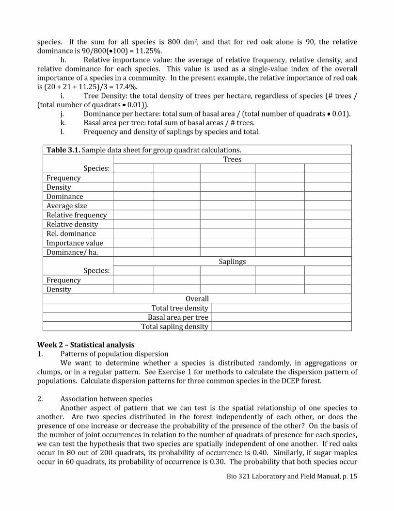
j. Dominance per hectare: total sum of basal area / (total number of quadrats 0.01). k. Basal area per tree: total sum of basal areas / # trees. l. Frequency and density of saplings by species and total.
Table 3.1. Sample data sheet for group quadrat calculations.
Species:
Trees
Frequency Density Dominance Average size Relative frequency Relative density Rel. dominance Importance value Dominance/ ha.
Species:
Saplings
Frequency Density
Overall Total tree density
Basal area per tree Total sapling density
Week 2 – Statistical analysis 1. Patterns of population dispersion We want to determine whether a species is distributed randomly, in aggregations or clumps, or in a regular pattern. See Exercise 1 for methods to calculate the dispersion pattern of populations. Calculate dispersion patterns for three common species in the DCEP forest. 2. Association between species Another aspect of pattern that we can test is the spatial relationship of one species to another. Are two species distributed in the forest independently of each other, or does the presence of one increase or decrease the probability of the presence of the other? On the basis of the number of joint occurrences in relation to the number of quadrats of presence for each species, we can test the hypothesis that two species are spatially independent of one another. If red oaks occur in 80 out of 200 quadrats, its probability of occurrence is 0.40. Similarly, if sugar maples occur in 60 quadrats, its probability of occurrence is 0.30. The probability that both species occur
Bio 321 Laboratory and Field Manual, p. 16
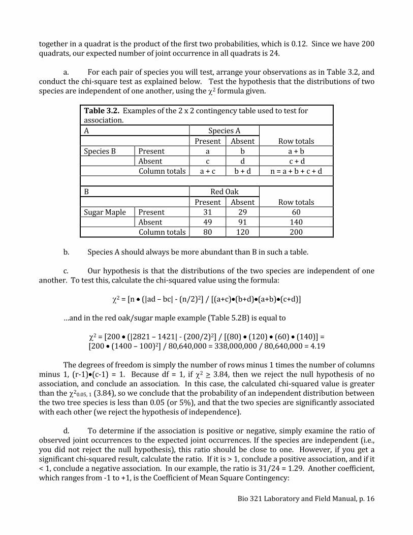
together in a quadrat is the product of the first two probabilities, which is 0.12. Since we have 200 quadrats, our expected number of joint occurrence in all quadrats is 24. a. For each pair of species you will test, arrange your observations as in Table 3.2, and conduct the chi-square test as explained below. Test the hypothesis that the distributions of two species are independent of one another, using the 2 formula given.
Table 3.2. Examples of the 2 x 2 contingency table used to test for association.
A Species A
Present Absent Row totals Species B Present a b a + b Absent c d c + d
Column totals a + c b + d n = a + b + c + d
B Red Oak
Present Absent Row totals Sugar Maple Present 31 29 60 Absent 49 91 140
Column totals 80 120 200
b. Species A should always be more abundant than B in such a table. c. Our hypothesis is that the distributions of the two species are independent of one
another. To test this, calculate the chi-squared value using the formula:
2 = [n (|ad – bc| - (n/2)2] / [(a+c) (b+d) (a+b) (c+d)]
…and in the red oak/sugar maple example (Table 5.2B) is equal to
2 = [200 (|2821 – 1421| - (200/2)2] / [(80) (120) (60) (140)] = [200 (1400 – 100)2] / 80,640,000 = 338,000,000 / 80,640,000 = 4.19
The degrees of freedom is simply the number of rows minus 1 times the number of columns minus 1, (r-1) (c-1) = 1. Because df = 1, if 2 > 3.84, then we reject the null hypothesis of no association, and conclude an association. In this case, the calculated chi-squared value is greater than the 20.05, 1 (3.84), so we conclude that the probability of an independent distribution between the two tree species is less than 0.05 (or 5%), and that the two species are significantly associated with each other (we reject the hypothesis of independence). d. To determine if the association is positive or negative, simply examine the ratio of observed joint occurrences to the expected joint occurrences. If the species are independent (i.e., you did not reject the null hypothesis), this ratio should be close to one. However, if you get a significant chi-squared result, calculate the ratio. If it is > 1, conclude a positive association, and if it < 1, conclude a negative association. In our example, the ratio is 31/24 = 1.29. Another coefficient, which ranges from -1 to +1, is the Coefficient of Mean Square Contingency:

Bio 321 Laboratory and Field Manual, p. 17
CAB = ( 2/ (n + 2)) The association is concluded to be positive or negative using this coefficient if CAB is >0 or <0, respectively. 3. Community succession a. A very simple, and non-statistical, way we can determine if our forest is in a mature state, and predict the future composition of the forest, is to compare the present frequencies of trees to saplings. Prepare graphs illustrating the frequencies, densities, and dominance of each of three tree species compared to the same species of saplings. Questions and Report considerations For this first laboratory report, you will focus on a short Introduction, Results, Discussion, and Works Cited. You will need to present Results in graphical and tabular format. Decide which is best for each analysis you performed, as well as how best to condense and present the raw data (do not include Table 3.1 in your Results section). For the Discussion, put your results into the big picture, that is, relate our results to community composition, succession, and species associations. What did you notice when you were out in the forest? Have you determined what stage of succession the forest is in? Can you show that quantitatively? What are the major points you learned from this study? I will discuss the format of your Report in class, but review Sections 7 and 8 for formatting instructions and information on laboratory report preparation. Here are some additional questions and points to consider (these are suggestions and it is not required that you address each of these questions in the report): 1. Using basal area as an indicator of age and using sapling numbers, discuss age structure among the species in the sample. How would you present these data in a figure? Do so. 2. In our analyses, what are assumptions of each test? 3. What sampling errors, biases, or inconsistencies may be present? What abiotic factors may have changed as we sampled from one side of the forest to the other? 4. Predict what our plot might look like, in terms of species composition and dominance, in 100 years. On what do you base your prediction? 5. Discuss associations, positive or negative, among tree species. First, what did you find, and second, why do you suppose any two tree species have an association?

Bio 321 Laboratory and Field Manual, p. 18
5: Models and Theoretical Ecology
Introduction Many of the processes of population growth are difficult to observe in nature, especially among larger, longer-lived organisms. Computer simulations offer an excellent opportunity to model some of the processes we will discuss in lecture. We will use two programs, Microsoft Excel, with which you are probably familiar, and STELLA, developed by ISEE Systems. STELLA is an icon-based, conceptual, diagrammatic program that allows you to develop theoretical models without having to figure out the mathematical equations behind your model. The program is available on all the computers in the Ecology and Biostatistics laboratories. We will use a variety of features in Excel to develop models related to population growth and community dynamics, in order for you to learn how the models work, the concepts behind the models, and to become more familiar with using Excel to do your dirty work for you. Excel Models From the book Spreadsheet Exercises for Ecology and Evolution I’ve chosen several models for us to work on – they are the geometric model of population growth, demographic stochasticity, island biogeography, metapopulation dynamics, and source-sink population dynamics. There will be a packet of instructions passed out to you in class with directions for each on. Each of you, independently, will complete the geometric model of population growth, and then you will complete one other model assigned to you. For each of the two models you complete, be prepared to discuss with me your model, the theoretical background of the model, and the answers to the questions at the end of the chapter. Basics of STELLA STELLA is a computer software program that allows users to model different processes, including many of the ecological processes we have encountered and will encounter. While the mathematics behind some of the models we will discuss are beyond the scope of this course, STELLA uses a fairly straightforward schematic approach that puts the mathematics behind the scenes and focuses on the connections and interactions between components of the model. Map/Model Level STELLA opens in this level. There are a number of different building blocks you use to construct models to test hypotheses. Each building block in the Map/Model Level is briefly described below, and you will need to understand them to begin model building. In this level you can view Map or Model modes. They both show the same basic view, but the Model mode is where you build your equations. To switch between the two, click the icon on the left side of the window that shows either a small picture of Earth (Map mode) or the chi-square symbol ( 2 – Model mode). 1. Stocks: Stocks are accumulations of physical and non-physical stuff. They collect whatever
flows into and out of them. For our purposes, a stock might be a population, collecting and losing individuals via birth and mortality, respectively, or an island, collecting and losing species via colonization and extinction. To select a stock, click on the stock icon, which looks like a rectangle, by clicking once on the icon in the Building Block palette. Move the mouse to the desired location on the diagram and click to deposit the stock. Stocks may be Reservoirs or Conveyors. The default stock type is the Reservoir. Think of a Reservoir as a pool of water, or as an undifferentiated pile of “stuff”. A Reservoir passively accumulates its inflows, minus its

Bio 321 Laboratory and Field Manual, p. 19
outflows. Any units that flow into a Reservoir will lose their individual identity. Reservoirs mix together all units into an undifferentiated mass as they accumulate. Conveyors are similar except they move units out at regular intervals. Each unit remains in the conveyor stock for a specified period of time. If you double click on a stock in the Model mode you’ll note that the expression in the equation box requires an initial value for the stock. This value is evaluated at the outset of a simulation run.
2. Flows: The job of flows is to fill and drain stocks. The unfilled arrowhead on the flow pipe indicates the direction of the flow. Select the flow icon (horizontal arrow with circle underneath) by clicking once on the icon in the Building Block palette. Move the mouse to the desired starting location on the page, click-and-hold, and drag the cursor to the place where the flow will end. Release the click. As you drag, the flow will follow your cursor movement. To draw an outflow from a stock, be sure to start with the cursor inside of the stock. If you are not within the boundary of the stock when you begin dragging, your flow will be drawn with a cloud at its source. To draw an inflow to a stock, make sure that your cursor makes contact with the stock before you release your click. The stock will turn gray on contact to let you know to release your click. If you release the click prematurely, a cloud will appear at the destination end of the flow pipe. To replace a cloud with a stock, select the stock with the Hand tool. Drag the stock over the cloud. When the cursor (the tip of the index finger on the hand) is directly atop the cloud, the cloud will turn gray. Release your click, and the flow will be connected to the stock. The cloud will disappear. Flows may be uniflow or biflow. With uniflows, the flow volume will take on non-negative values only. On the other hand, biflows can take on any value. If you specify a flow as a biflow, a second, shaded arrowhead will appear on the flow to point the direction of negative flow. It is not possible to have a biflow connected to a conveyor. When the flow is conserved (i.e., it connects two stocks), the unit conversion check box is enabled. Unit conversion enables you to convert the units of measure for the flow, as material moves through the flow pipe. Unit conversion is useful in modeling processes such as predator/prey interactions that transform prey items into predator offspring, or chemical processes that involve molecular transformations. When you specify a flow as unit converted, a shaded half-circle will appear in the flow regulator on the diagram to indicate that unit conversion is taking place. When Unit conversion has been checked, an additional field will appear in the flow dialog. The inflow multiplier can be a number. Alternatively, it can be some model variable that appears in the Required Inputs list. What comes out of the upstream stock will be multiplied by the inflow multiplier, and then added to the downstream stock. At run time, the software will report the values for the flow, before unit conversion has taken place. Double click the flow while in the Model mode to access the equation editor. The Required Inputs list contains all inputs that have been connected to the flow using connectors. Anything in the Required Inputs list must be used in the equation definition for the flow.
3. Converters: The converter serves a utilitarian role in the software. It holds values for constants, defines external inputs to the model, calculates algebraic relationships, and serves as the repository for graphical functions. In general, it converts inputs into outputs, hence, the name converter. Select the converter icon (the circle) by clicking once on the icon in the Building Block palette. Move the mouse to the desired location and click once to deposit the converter.
4. Connectors: As its name suggests, the job of the connector is to connect model elements.

Bio 321 Laboratory and Field Manual, p. 20
Connectors have limitations in terms of what things they can connect. For instance, you can never drag a connector into a stock. The only way to change the magnitude of a stock is through a flow. Select the connector icon (the diagonal arrow) by clicking once on the icon in the Building Block palette. Slide the cursor to the place where the connector will start. This starting place must be within the boundary of a stock, flow regulator, or converter on your screen. Click-and-hold, and drag the cursor to the target converter or flow regulator. When you make contact, the target will turn gray. Release your click. In drawing connector linkages, you may encounter an alert that tells you that circular connections are not allowed. This alert means that you have attempted to create a chain of converters and/or flows, such that one converter or flow ultimately depends upon itself. The software cannot resolve the resultant simultaneous equations. To resolve the situation, you must include a stock somewhere in the chain.
5. Decision Process Diamond: This is not really a building block. It is a space saving device that serves to reduce clutter in your diagram. Whenever you have a mildly elaborate chain of logic that’s associated with making a decision, it’s usually a good idea to place it within a diamond. The diamond then opens to reveal a subspace into which you can place the associated logic of a particular process. You probably won’t have occasion to use these too much, depending on the complexity of your model.
Interface & Equation Levels You won’t use these levels too much, although the Equation Level is used to view the equations that STELLA has constructed for your model. You do not need to construct equations; STELLA does that for you. Dynamite If you put in an icon that you realize you don’t want, click on the stick of dynamite, then click on the offending icon and it will be blown to bits. Run Model As you construct a model, STELLA is busy behind the scenes writing equations based on the picture you are creating. To complete the conversion of a picture to computer simulation model you need only click in a few simple equations, sketch some curves, and enter a few numbers. Click the Map/Model toggle to begin this process. As you do this, run your model to see what it’s doing. When you simulate your STELLA models you can view output in several ways, including animation, a graph over time, and a table of numeric values. Under the Run Menu, click Run Specs… to specify the length of the simulation, the unit of time, and the frequency of calculation. DT is the fraction of one unit of time that passes before STELLA performs another iteration. The default value is 0.25, which means that if the unit of time is days, the model’s equations are recalculated four times a day, each time using new values from the previous iteration. Click on Run to run the model, but first open a graph and/or a table. The icons to control graphs and tables are to the right of the building blocks and look like a graph and a table. Select one or both, and click in the window to place the object. Double-click on it to specify what parameters you want to graph or tabulate. Select the parameter in the “Allowable” window and then click on the arrow to place it in the “Selected” window. Then any time you run the model, those parameters will be graphed, whether the pad is open or not. You can later open the graph/table pad to view the results.
Bio 321 Laboratory and Field Manual, p. 21
Population Growth of White-tailed Deer For this exercise, we will first start by developing some simple population growth models, and then increase their complexity and, hopefully, their realism. The simplest population growth model is one of Density Independent Growth, which examines how populations grow when the density of that population does not affect the growth of the population. The model you build should yield a graph of exponential population growth. a. Place a stock in the middle of the window. Highlight it and type “Deer Population.” Place a flow starting outside the stock and flowing into it. Name it “births.” Finally, Place a converter near the flow and call it “birth fraction.” We will multiply the population in the stock by the birth fraction to yield the flow of new births into the stock. That is how the population will grow, and its rate of growth will depend on the birth fraction. In order to do this, we need to add a couple of connectors. b. Add two connectors, one starting from birth fraction and one from deer population and both ending at births. You may notice that there are question marks in each of the building blocks (if you’re in the Model mode), which indicates that you need to add some information to them. Double-click on deer population and enter 100 as the initial value. Double-click on birth fraction and enter 0.2 as the “right-hand side of the equation.” Double-click on births. In the required input box, click on deer population and that term will appear in the window at the bottom. Type an asterisk next to that term and click on birth fraction above. Now the window at the bottom should read: deer population*birth fraction. The model is complete. c. Place a graph and a table in your window, double-click to open them, and select all three terms to graph and tabulate. You really don’t need to graph birth fraction because it is a constant, but it is good to make sure it was actually put in as a constant. d. Run the simulation. Then click on Run Specs… in the run model window. Change the length of the simulation to 25 years. What is the population size in year 10? In year 20? What is the shape of the curve? Density Dependent Population Growth This simulation explores how populations grow when the density of that population affects the growth rate of the population. There are a couple of different ways we could model density dependence. We will all do one together, and then you and your group can work through another. The thing you may have noticed about the first model is that all individuals are apparently immortal. Let’s add some death to our deer population. a. Now that you know something about modeling, add a flow from the population, a converter, and three connectors, one from the stock to the outflow, one from the stock to the converter, and another from the converter to the outflow. Call the outflow “deaths” and the converter “death fraction.” b. We will make the death fraction dependent on the deer population. Open up death fraction and make it equal to deer population. Click “become equation” and we will make a graph of death fraction vs. deer population. As the deer population becomes larger, death rate, or death fraction increases. You should make the curve S-shaped; you can draw in a graph right on
Bio 321 Laboratory and Field Manual, p. 22
the grid, or you type numbers into the table on the right. Scale the death fraction from 0-0.2, since it is per capita death rate. Scale the deer population however large you want. c. Run the model. What happens to the population growth curve? What is the shape of the population growth curve? Save your model and show it to me during class; part of your participation grade will be based on your model construction. d. Make the model more complex and realistic by adding some stochasticity (variability) into the model. Not every individual will reproduce in any given year, and not every year will produce the same per capita population growth. We will discuss at least two ways to introduce variability into intrinsic birth and death rates. Consider what happens to your population, and again save this model and review it with me. Multi-Species Interactions The appealing thing about STELLA is that you can model just about anything you want, from a simple model of money flowing into and out of your checking account to the entire biosphere (a daunting challenge to say the least). You are only limited by your knowledge of the particular system and your imagination and creativity. The first simulation examined a simple population growth curve, which we made more complex as we went along. Now, build on population growth model by adding in at least one interaction, either between the deer and a predator or between the deer and its food source or both. Use a population approach, as we did above, to determine the effects of population size of prey on the population growth of a predator or the vegetation prey consume. You can consider the entire community of vegetation as your “population” or you can separate out different types of vegetation. You can use different predators, or include humans in the interaction scheme. You and your partner must consider carefully what it is you will model, and in the course of developing a model, you will be able to test the effects of different parameters on the growth of populations. Alternatively, you can take a similar approach to model the changes in an entire community on an island or some other ecosystem. a. Use an approach similar to the one above to model the predator or the vegetation, but now you need to connect the prey population to this new model. We’ll discuss different ways to connect the deer population to the other population(s) you and your partner are modeling. b. Do you think your model is realistic? What other information are you lacking that prevents you from making a more realistic model? c. You will e-mail this model to me prior to presenting it in class. Before you e-mail it to me, be sure you have graphed the populations or communities, and set the time specs so the model runs for 100 years. Indicate in a comment box what special features you’ve used and the answers to the questions above. Add a comment box by clicking the “A” in the button bar and then clicking somewhere in the model (preferably in the upper left so I can find it and you can explain it to the class easily).
Preparation of Oral Presentations This second oral presentation will be prepared with your partner, and presentations will be given the final week of lab. You will explain the theory behind your model, how you constructed it, the different components you included, how it works, and what results you obtained when you ran the model. Consult Section 9 for guidelines and suggestions for presentations.
Bio 321 Laboratory and Field Manual, p. 23
6: Diversity of Stream Insect Communities Introduction
Benthic macroinvertebrates are common inhabitants of lakes and streams where they occupy varied trophic positions in food webs and help cycle nutrients. "Benthic" means "bottom-living", so these organisms usually inhabit bottom substrates for at least part of their life cycle; the prefix "macro" indicates that these organisms are retained by mesh sizes greater than 200 mm.
The most diverse group of benthic macroinvertebrates is the aquatic insects, which
account for about 70% of known species of aquatic macroinvertebrates. As a highly diverse group, benthic macroinvertebrates are excellent candidates for studies of changes in biodiversity. Qualitative sampling is possible using simple, inexpensive equipment, good taxonomic keys are available, and methods of data analysis are well developed.
However, keep the following in mind when working with benthic macroinvertebrates.
First, quantitative sampling is difficult because the clumped distribution of benthic macroinvertebrates requires large numbers of samples to achieve precision in estimating population abundance. Second, the distribution and abundance of macroinvertebrates are affected by a large number of natural factors, which have to be accounted for to determine changes in biodiversity. Finally, some groups of benthic macroinvertebrates are taxonomically difficult, so we will only identify our animals to the order or family level.
The collection of benthic macroinvertebrates from streams is usually a straightforward procedure using standard equipment. However, the removal of organisms from background material can be tedious and time-consuming unless available laborsaving strategies are used. Data-analysis procedures are standard, and can be done by anyone trained in elementary statistics. The methods below describe sampling methods for benthic macroinvertebrates in lotic (stream) habitats, different types of analyses, and techniques for efficient operation in the field and laboratory.
Abiotic Factors
Our sampling study will characterize two habitats using a variety of abiotic factors: (1) site variables such as land use, water depth, and substrate composition; and (2) water variables such as pH, conductivity, and temperature. The following describes a few variables that can be easily measured in streams and should be part of general biodiversity sampling for benthic macroinvertebrates.
1. Area and site variables It is often useful to photograph or describe a site to provide a record of the area and land
use. Descriptions should be detail canopy coverage over a stream, algal coverage in the water, or the extent and type of vegetation in the riparian zone. One should also describe the riffle-pool sequence and note whether samples were taken from riffles or pools. See the data sheets at the end of the chapter for details on information to collect.
2. Stream physical and chemical factors Physical and chemical factors of the environment are among the strongest determinants of benthic macroinvertebrate community structure. Substrate is perhaps the most important
Bio 321 Laboratory and Field Manual, p. 24
environmental factor for benthic macroinvertebrates and so it needs to be adequately described. A number of methods using weights of various substrate fractions after sieving are available, but relative descriptions will suffice for our survey. In streams, substrate score is determined by the sizes of the two predominant substrates, and the size of the material surrounding the predominant substrates. For instance, you may find boulders and large stones to be the predominant substrate, with small gravel or sand interspersed between the predominant substrate. We will estimate the percentage of different sizes as described on the data sheet at the end of the exercise.
In addition to pH, conductivity, and temperature, measurements of dissolved oxygen and alkalinity should be considered. All of these variables will be measured using portable field instruments or kits. Week 1 – Materials pH meter conductivity meter dissolved oxygen meter measuring tape water velocity meters chemistry test kits D-frame nets waders/boots sample bottles 70% ethanol enamel or plastic pans forceps squirt bottles with EtOH squirt bottles with water Week 1 – Methods for Data Collection
This protocol applies to many sampling situations for benthic macroinvertebrates in wadeable streams, and is designed to integrate different habitats within a stream reach (e.g., see Cuffney et al. 1993). The majority of animals in fast-flowing streams will be underneath stones. We’ll use a D-frame, or kick, net and distinguishes four habitats: (1) steep banks/vegetated margins, (2) silty bottom with organic matter, (3) woody debris with organic matter, and (4) sand/rock/gravel substrate. We will probably only sample two to three of these habitat types. The kick net is placed on the streambed against the flow and the substrate upstream from the net is agitated. Animals living in this agitated substrate are dislodged and flow into the net. The kick net is so-called because the most common way to agitate the streambed is by kicking the stones or sediment. However, be aware that extreme agitation may damage specimens to the point of being unidentifiable. Also be aware that this method may not collect all individuals in the portion of streambed being sampled, but will be useful for comparative purposes.
a. As a class, we’ll collect information on stream physical and chemical parameters.
Data from all sections will be pooled prior to next week's lab period. First, we need to characterize habitat variables, as described above. You should take notes on these variables in your notebook or in the data collection sheets at the end of the exercise.
b. We’ll also characterize the stream channel itself. The size and shape of the
channel, and the substrate paving its bottom (a factor of critical importance to the benthos) are a result of the geology of the area and peak flows. Peak flows are related to summer rainstorms. Erodible materials are carried through the stream, shape the width and depth of the channel, and leave behind material that the stream does not have enough energy to transport. It is possible to relate faunal distributions to a particular suite of hydrological variables by measuring or taking note of channel characteristics (Cobb et al. 1992).
c. Next, collect three water samples, at random, from the stream. We will then
Bio 321 Laboratory and Field Manual, p. 25
measure each water chemistry parameter on each sample. Work in groups of four, so that everyone can observe and/or assist in the determination of each parameter. The instructions for each instrument or kit will be described by the instructor or are described with the kit itself. Follow the instructions carefully and record the data in your data sheet.
d. Next, select three sites for macroinvertebrate sampling. At each site one group will
measure surface and bottom water velocity, water depth, and describe the substrate at that spot. Do not step in or otherwise disturb the site prior to sampling!
e. Place the kick net at the selected site, with the flat side resting on the substrate of
the stream, downstream of the designated kicker who is standing still on the site. For large rocks, the net is held downstream while the rock is brushed by hand. The net is held near the area being disturbed and up against the substrate, so dislodged animals will be carried into the net. The collector will spend a designated period of time, 1 minute, disturbing the area between 0 and 1 meter upstream from the net, using hands or feet.
f. When sampling is completed, lift the net out of the water, moving it upstream as
you do. You can use the current of the water to wash much of the material down into the bottom of the net. Now slowly begin to invert the net, scanning the interior as you go. If you see any living animals, gently pry them off the net with forceps and place them in an enamel pan with a bit of 70% ethanol. When you get to the bottom of the net, all the material at the bottom can be dumped into the pan. Carefully rinse the inside of the net with a squirt bottle of ethanol to get all the material off the net.
g. The entire sample, sand, insects, leaves, and all, should then be poured into a
sample bottle. Label the container with your group members, the date, and the location. Place the containers in the cooler provided for transport back to the laboratory. Week 2 – Materials insect identification keys 10% MgSO4 forceps enamel or plastic pans sieves dissecting microscopes petri dishes plastic pipets calipers Week 2 – Sample Processing and Sorting
a. We’ll spend most of this week sorting our samples. You and your mates can split up the sample by pouring portions of it into different enamel pans. Scan your sample for preserved animals, carefully sorting the sample and teasing apart any large debris. Place your insects into a petri dish or small watch glass with a small amount of 70% ethanol.
b. When you can't find any more animals and all large debris has been removed, pour
your sample into a large beaker and fill the remainder of the beaker with 10% magnesium sulfate. This will cause most organic matter to float to the top. When you have retrieved most of the floating animals, run the sample through a sieve in the sink, and dump the debris in the trash.
c. Keep accurate counts of all insects found in the data sheets. Next, separate the
insects into groups of anatomically similar specimens. Use the pictorial keys provided to identify each specimen at least to the order. For two groups, the mayflies (Order Ephemeroptera) and the flies (Order Diptera), we will attempt to identify most of our specimens to the family level,

Bio 321 Laboratory and Field Manual, p. 26
counting the number of different families we find and the number of individuals of each family. Week 3 – Data Analysis
Four different types of biodiversity studies may be undertaken: (1) pilot studies at the beginning of a full-fledged program; (2) descriptions of population or community characteristics; (3) detection of differences in communities between or among sites; and (4) initiation of a long-term, rapid-assessment program. Each of these studies has its own data-analytical requirements, so identification of objectives of a biodiversity study is critical to experimental design. Our project is a community comparison of two streams.
a. Using Excel we will calculate a couple of indices of biodiversity and stream health,
and perform correlations among physical, chemical, and biological data. We must first enter all the data into the spreadsheet, as a group, although your instructor will have entered some of it. Calculate total abundance of insects and enter those values for each site into your spreadsheet.
b. Next, calculate biodiversity using the Shannon index, which is H' = - piln(pi),
where pi is the proportion of individuals found in the ith species and ln is the natural logarithm of the proportion. Normally, this index is used for individual species, but we will calculate it for the number of taxa we have at the order level. We lose a lot of information, but we cannot identify all our insects to the species. Values of the Shannon diversity index often fall between 1.5 and 3.5. The index is affected by both the number of species (or orders in our case) and their evenness (how they are distributed). We’ll calculate diversity for each sample, and overall diversity for pooled samples. Examine these numbers carefully for deviations of samples from pooled diversity. Do any sites that deviate have any differences in physical or chemical parameters?
c. Another index we can calculate is the EPT index, which is a ratio of three orders, E
= Ephemeroptera (the mayflies), P = Plecoptera (the stoneflies), and T = Trichoptera (the caddisflies), to one family of Dipterans, Family Chironomidae (the midges). These EPT orders tend to be more sensitive to pollution than chironomids. The creation of one quantitative measure used to compare the streams makes the analysis simpler. What is one drawback of reducing data down to one or a few numbers?
d. Another index is the ratio of the number of individuals of the dominant group to total numbers of individuals in each sample. Calculate this value for each site.
e. Similarity indices are often used to compare two sites, and are simple measures of
the extent to which two habitats have species (or taxa) in common. We will use an index called the Morisita-Horn Coefficient of Similarity, which takes into account both sample size and species (or taxa) richness. It ranges from 0 (completely dissimilar) to 1 (completely similar), and is calculated using the following equation:
[2 (nia nib)] CMH = ------------------------------
[(da + db) Na Nb]
where Na and Nb = total number of individuals in sites a and b, respectively, nia and nib = the total number of individuals in the ith species in sample a and b, respectively, and

Bio 321 Laboratory and Field Manual, p. 27
da = [ (nia2)] / Na2 (use similar equation for site b). Use Table 4.1 to practice calculating the index. Some calculations are done for you.
Table 4.1. Sample data used to calculate the Morisita-Horn Coefficient of Similarity (CMH). Use the space in the last row to calculate CMH. Order nia nib nia x nib nia2 nib2 Ephemeroptera 85 55 4675 7225 3025 Plecoptera 43 5 215 Trichoptera 32 3 96 Chironomidae 10 75 750 Diptera 47 15 705 Odonata 9 12 108 Oligochaeta 5 3 15 Coleoptera 3 0 0 Sums 6564 Na Nb Na2 Nb2 234 169 54756
d (a or b) 0.23 C
f. Finally, determine the Habitat Assessment Score on the last page of the Evaluation
Sheets. Compare the values for the sites. This Score is determined by physical characteristics of the streams and riparian zones. We can also examine correlations among various physicochemical parameters and the biological data. For instance, is stream velocity correlated with total number of insects or type of substrate? There are many different correlations we can make, but you should attempt to find correlations that you think are interesting or relevant. We will discuss these correlations and how to calculate them in class. References Cobb DG, Galloway TD, & Flannagan JF (1992) Effects of discharge and substrate stability on density and species
composition of stream insects. Canadian J. of Fisheries & Aquatic Sciences 49:1788-1795. Cuffney TF, Gurtz ME & Meador ME (1993) Methods for collecting benthic invertebrate samples as part of the
National Water-Quality Assessment Program. U.S. Geological Survey Report 93-406. U.S.G.S., Raleigh, North Carolina. 65 p. (http:// wwwrvares.er.usqs.gov/nawqa/protocols/OFR-93-406/inv1.html).
Preparing Your Report We will discuss the results at the end of laboratory, as time permits. The format of the report will be similar to that for previous reports. Review Sections 7 and 8 for formatting instructions and information on laboratory report preparation. Basic Guidelines for Writing 1. Prepare tables and figures. Identify key points. 2. Prepare an outline structured around key points and the big picture. 3. Save your work often and in more than one place. 4. Prepare a rough draft that can be checked, read aloud, altered, and rewritten. 5. Rewrite to make your writing straightforward and concise.

Bio 321 Laboratory and Field Manual, p. 28
6. Prepare a draft (the “first draft”), which can be turned in to the instructor. Introduction Introduce the question, the hypotheses, the motivation, the justification, and the study organisms in this section. Why did we do this exercise? What is the larger context in which we can place this study? Be brief, but thorough. See Section 7 for an example of a Report. Brief Methods Since the detailed methods are in this manual, there is no need to repeat what is here. You should state the general method used to sample streams and where you performed the experiment. Refer to this laboratory manual to cite complete methods (i.e., Paradise 2005). Results Decide whether graphs or tables are best for each aspect of your data presentation and analysis, as well as how best to condense and present the data. By now, you should be familiar with how to prepare a professional grade Results section. Show the data that relate to your hypotheses and questions and that make specific points. Each finding should be briefly described; save discussion of the significant conclusions for the next section. The objective here is to describe in a clear and logical way what you discovered. YOU MUST PROVIDE TEXT, NOT JUST TABLES and FIGURES! Include at least two separate figures – see Section 6. Present these in the form of line graphs or histograms, whichever is most appropriate. Calculate measures of variation (e.g., standard deviation) and include them. Tables and figures should always be labeled with a number, such as "Table 1" or "Figure 3." Title and label your graphs and tables so the reader knows what they are examining. Include the results of statistical analyses, using tables or figures. Discussion: Put your results into the big picture. What are the major points you learned from this study? Examine the major concepts illustrated by the experiments. Point out why the research was significant, what general conclusions can be drawn, and the relation between your findings and basic scientific principles and concepts. Consider the following questions: Why did we do this exercise? What is the larger context in which we can place this study? How do your results support our hypotheses? What new questions arise after examining the results? How does the study relate to ecology in general? References You will need to cite the Laboratory Manual, the textbook, or some primary literature that you’ve read while preparing this report. Include complete citations of any works you cite; do not list sources that are not cited in the body of the report. Use a standard citation format. See me for references that have no analogous example listed.

Bio 321 Laboratory and Field Manual, p. 29
Sample Site Evaluation Sheet Date: SITE DESCRIPTION, LOCATION, AND ACCESSIBILITY Stream: Watershed: Town/County:
Site Location, directions to site (include important landmarks), accessibility (explain steep banks, poison ivy, etc.):
SECTION I: BACKGROUND INFORMATION Site Number (on this stream): _______ Time: ________ Investigators: __________ Estimated Elevation: _____ Photos/Site Record: __________ Comments:
Weather Now Last 48 hrs ____ ____ Clear/Sunny ____ ____ Overcast ____ ____ Showers ____ ____ Rain (steady) ____ ____ Storm (heavy)
STREAM CHARACTERISTICS Stream habitat: Riffle ____ Glide ____ Pool _____ (check if present) small surface waves smooth moving water still water
Stream Bottom (estimate % in each category, according to size of particles): _____ _____ _____ _____ _____ _____ % bedrock % boulder % cobble % gravel % sand % silt (>25cm) (5-25cm) (0.25-5cm) (0.1-0.25cm) (<0.1cm) Embeddedness: _______% (area of particles > gravel surrounded/covered by sand/silt) Flow meter and depth readings at 2 fast sites: Flow: 1: _____ 2: _____ Avg: ______Depth: 1: _____ 2: _____ Avg: ______ Flow meter and depth readings at 2 slow sites: Flow: 1: _____ 2: _____ Avg: ______Depth: 1: _____ 2: _____ Avg: ______ Stream Width (3 measurements) 1: _____ 2: _____ 3: _____ Avg: ______ SECONDARY HABITAT CHARACTERISTICS 1. Velocity/Depth Regime ______ slow-deep ______ slow-shallow (check if present) ______ fast-deep ______ fast-shallow (deep = >2’) 2. Do the banks or channel appear to be altered? _______ (Y or N) _______% Left bank altered (facing upstream) ______% Right bank altered 3. Abundance of sediment deposits in pools ______ High ______ Moderate ______ Slight ______ None
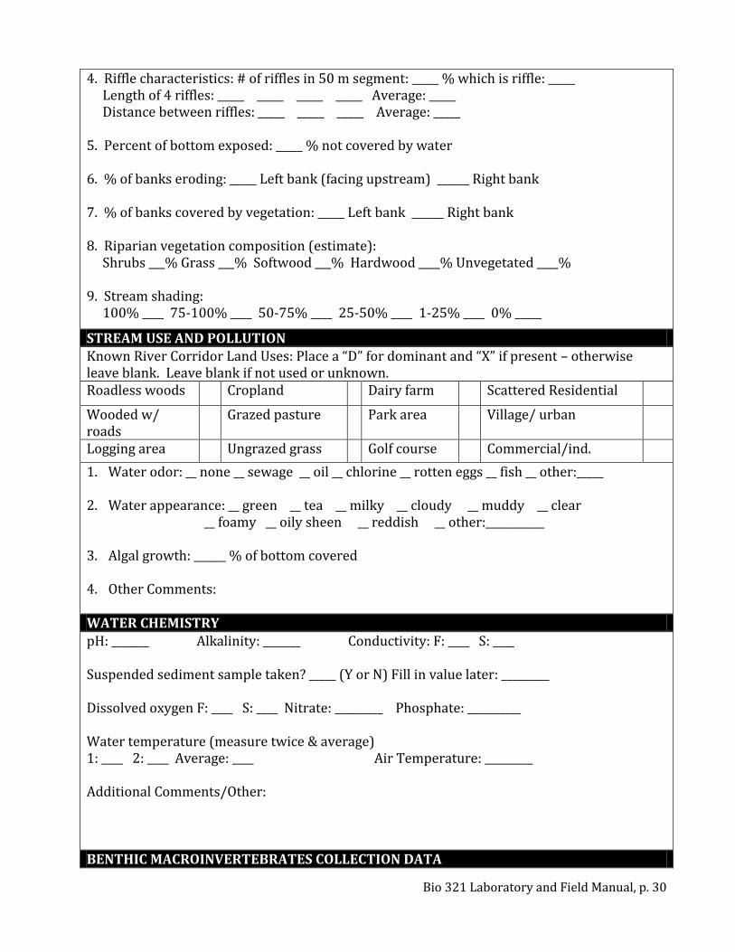
Bio 321 Laboratory and Field Manual, p. 30
4. Riffle characteristics: # of riffles in 50 m segment: _____ % which is riffle: _____ Length of 4 riffles: _____ _____ _____ _____ Average: _____ Distance between riffles: _____ _____ _____ Average: _____ 5. Percent of bottom exposed: _____ % not covered by water 6. % of banks eroding: _____ Left bank (facing upstream) ______ Right bank 7. % of banks covered by vegetation: _____ Left bank ______ Right bank 8. Riparian vegetation composition (estimate): Shrubs ___% Grass ___% Softwood ___% Hardwood ____% Unvegetated ____% 9. Stream shading: 100% ____ 75-100% ____ 50-75% ____ 25-50% ____ 1-25% ____ 0% _____
STREAM USE AND POLLUTION Known River Corridor Land Uses: Place a “D” for dominant and “X” if present – otherwise leave blank. Leave blank if not used or unknown. Roadless woods Cropland Dairy farm Scattered Residential
Wooded w/ roads
Grazed pasture Park area Village/ urban
Logging area Ungrazed grass Golf course Commercial/ind.
1. Water odor: __ none __ sewage __ oil __ chlorine __ rotten eggs __ fish __ other:_____ 2. Water appearance: __ green __ tea __ milky __ cloudy __ muddy __ clear __ foamy __ oily sheen __ reddish __ other:___________ 3. Algal growth: ______ % of bottom covered 4. Other Comments: WATER CHEMISTRY pH: _______ Alkalinity: _______ Conductivity: F: ____ S: ____ Suspended sediment sample taken? _____ (Y or N) Fill in value later: _________ Dissolved oxygen F: ____ S: ____ Nitrate: _________ Phosphate: __________ Water temperature (measure twice & average) 1: ____ 2: ____ Average: ____ Air Temperature: _________ Additional Comments/Other: BENTHIC MACROINVERTEBRATES COLLECTION DATA

Bio 321 Laboratory and Field Manual, p. 31
Replicate #: 1 Total number of organisms picked _____ Number of Orders: ______ Families: ______ Date sorted: _____ Sorting notes: Names of sorters: __________________ Names of identifiers: ___________________ Identification Comments: Replicate #: 2 Total number of organisms picked _____ Number of Orders: ______ Families: ______ Date sorted: _____ Sorting notes: Names of sorters: __________________ Names of identifiers: ___________________ Identification Comments: Replicate #: 3 Total number of organisms picked _____ Number of Orders: ______ Families: ______ Date sorted: _____ Sorting notes: Names of sorters: __________________ Names of identifiers: ___________________ Identification Comments: IDENTIFICATION AND ENUMERATION SECTIONS: ORDER LEVEL
Abundance (A) for each rep Richness (S) for each replicate Selected Major Groups 1 2 3 Avg. 1 2 3 Avg.
Mayflies
Stoneflies
Caddisflies
Chironomid Midges
Beetles
TOTAL (Selected)
Other Major Groups 1 2 3 Avg. 1 2 3 Avg.
Other True Flies
Dragon/Damselflies
Dobsonflies/Alderflies
Non-Insect Inverts.
Other:
Other:
TOTAL (Other)

Bio 321 Laboratory and Field Manual, p. 32
IDENTIFICATION AND ENUMERATION SECTIONS: FAMILY LEVEL
Replicate # 1 2 3
Families in Major Groups Tolerance A A A Avg. A FFG
EPHEMEROPTERA: Mayflies (not all families listed) Baetidae 4 GC/SC
Ephemerellidae 1 GC/SC
Ephemeridae 4 GC
Heptageniidae 4 SC/GC
Leptophlebiidae 2 GC
Oligoneuridae 2 FC
Siphlonuridae 7 GC
Total # of Families
Total Ephemeroptera
Replicate # 1 2 3
Families in Major Groups Tolerance A A A Avg. A FFG
DIPTERA: True Flies (not all families listed) Chironomidae 7 ALL
Dixidae
Empididae 6 PR
Ptychopteridae
Simuliidae 6 FC
Tabanidae 6 PR
Tipulidae 3 GC/PR/SH
Total # of Families
Total Diptera
Key: Tolerance = Family pollution tolerance level A = Abundance (# of individuals in family); Avg. = average abundance for 3 replicates FFG = Functional Feeding Groups: SC = scraper; FC = filtering/collector; GC = gathering collector; PR = predator; SH = shredder Note: designations are generalized for families. When species level information is available, these designations should be adjusted to reflect the FFG of the dominant taxon within the family or allocated among the FFG of the taxa actually present.
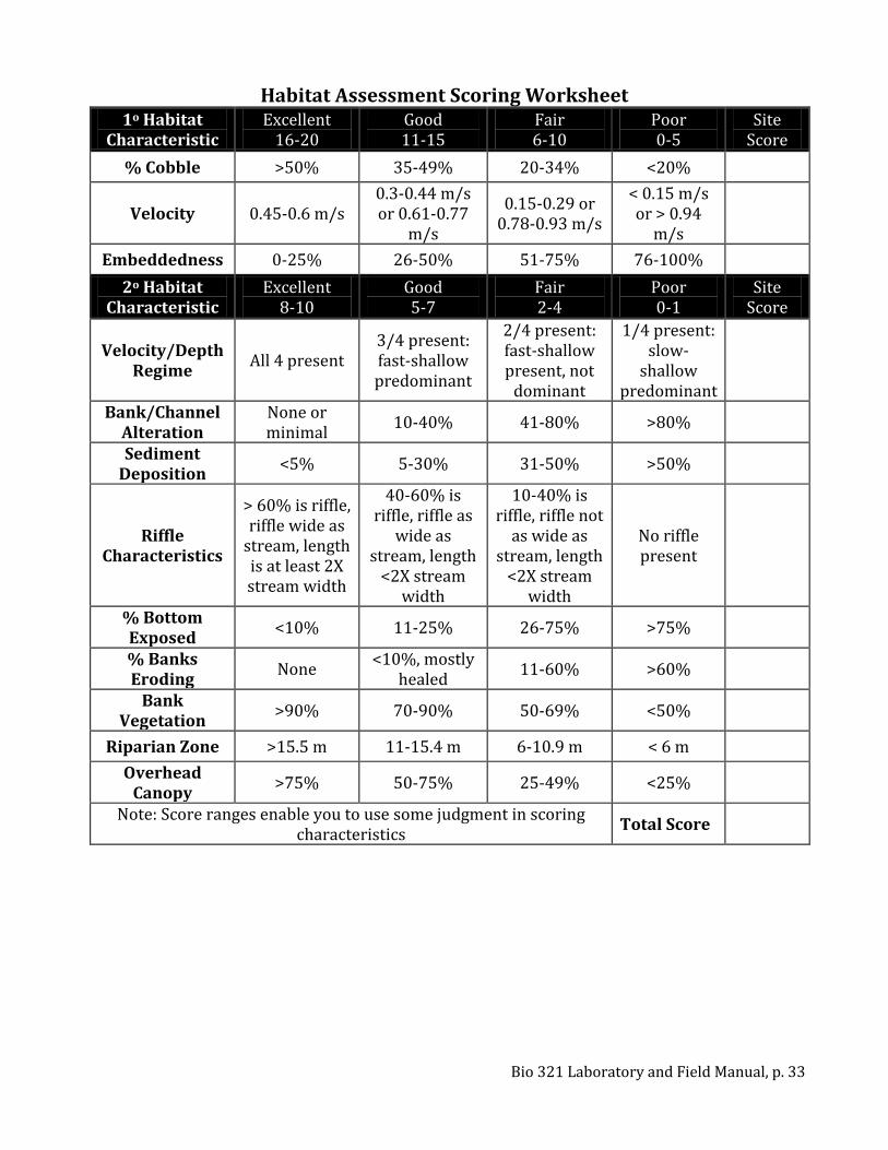
Bio 321 Laboratory and Field Manual, p. 33
Habitat Assessment Scoring Worksheet 1o Habitat
Characteristic Excellent
16-20 Good 11-15
Fair 6-10
Poor 0-5
Site Score
% Cobble >50% 35-49% 20-34% <20%
Velocity 0.45-0.6 m/s 0.3-0.44 m/s or 0.61-0.77
m/s
0.15-0.29 or 0.78-0.93 m/s
< 0.15 m/s or > 0.94
m/s
Embeddedness 0-25% 26-50% 51-75% 76-100%
2o Habitat Characteristic
Excellent 8-10
Good 5-7
Fair 2-4
Poor 0-1
Site Score
Velocity/Depth Regime
All 4 present 3/4 present: fast-shallow predominant
2/4 present: fast-shallow present, not
dominant
1/4 present: slow-
shallow predominant
Bank/Channel Alteration
None or minimal
10-40% 41-80% >80%
Sediment Deposition
<5% 5-30% 31-50% >50%
Riffle Characteristics
> 60% is riffle, riffle wide as
stream, length is at least 2X stream width
40-60% is riffle, riffle as
wide as stream, length
<2X stream width
10-40% is riffle, riffle not
as wide as stream, length
<2X stream width
No riffle present
% Bottom Exposed
<10% 11-25% 26-75% >75%
% Banks Eroding
None <10%, mostly
healed 11-60% >60%
Bank Vegetation
>90% 70-90% 50-69% <50%
Riparian Zone >15.5 m 11-15.4 m 6-10.9 m < 6 m
Overhead Canopy
>75% 50-75% 25-49% <25%
Note: Score ranges enable you to use some judgment in scoring characteristics
Total Score
Bio 321 Laboratory and Field Manual, p. 34
7. Preparing and Writing Scientific Research Reports Basic Guidelines for Writing Writing a paper on your observations, experiments, and conclusions is a critical part of a laboratory course in ecology. You should set aside whatever notions you may have about "scientific writing" and prepare reports that are composed of straightforward English-language sentences. Remember that the point of the report is to effectively convey a message to the reader. Decide what you want to say and then translate your mental notions into symbols that will have specific meaning for the reader. In this context, writing sentences that sound right is not merely a matter of aesthetics, but a way of promoting effective communication. Follow the organization suggestions below, and use the guidelines for each section to organize your paper. 1. Prepare your summary tables and figures. Identify the key points that you wish to make
and structure your paper around them. 2. Prepare an outline on a computer. The outline is the design of your paper. The more time you
take to construct it carefully, the more logical your paper will be and the easier it will be to turn the outline into text. Save your outline and first draft on disk, and save any early hardcopies you prepare. Be sure to save your work on more than one disk.
3. Prepare at least two drafts of text. First, prepare a rough draft that can be checked, read aloud, altered, and rewritten. The second draft may be ready for your instructor.
4. Avoid jargon as much as possible. State your meaning in a simple and concise manner. Whenever possible, remove unnecessary words from your sentences. Reading aloud helps identify unnecessary words and awkward phrases. Unnecessarily long sentences are ineffective because they dilute the writer's meaning. Economical sentences drive their messages home forcefully.
5. Use the “spell check” feature of your word processor! Use the “grammar check” too, if you feel inclined. By removing errors, you help the reader focus on your message, rather than by distracting them with your errors.
The Form of a Scientific Report Both tradition and common sense support the fundamental structure of scientific report consisting of an introduction, materials and methods, results, discussion, and references cited. In preparing your reports, you may work together in your groups to compare and compute results, but each individual must write their own section of the report. See Exercise 1 to help you decide how to prepare tables and graphs. 1. Introduction:
This is a statement of the purpose of the study. Introduce the problems and questions you addressed in your experiment (i.e., why did you do it?). You must also make a statement of your hypothesis or question. In a formal scientific paper, the author will usually review previous publications related to the hypothesis or question, in order to put their work in a larger contect. For our purposes, an introduction of 1-2 paragraphs should be sufficient. Use information from the lecture and your text to provide background (add a literature review if instructed to do so).
2. Methods and Materials: The purpose of this section is to allow the reader to critique or repeat the experiment performed. Usually you would address the following questions: What did we do? How did we do it? Where
Bio 321 Laboratory and Field Manual, p. 35
did we do it? What organisms did we study? What equipment did we use? How did we analyze the data? How did you set up your experiment? How many experimental groups did you have? How did you measure the effect you studied? For most exercises, however, the methods will be presented in this manual or by the instructor. To repeat them in your report would only be busy work. I will ask you only to describe materials and methods not included above or in another handout. Anything that is different from methods stated in the manual must be explicitly stated. Ask me if you have questions about any specifics. Sometimes materials and methods will not be required at all. 3. Results:
This section presents the key findings of the study, the results of experiments and field observation, and/or the data gathered during the project. Here you want to show data, in tables or graphs that relate to your stated hypotheses and questions and make specific points. Each finding should be briefly discussed and perhaps related to other results, although you should save discussion of the truly significant conclusions for the next section. The object here is to describe in a clear and logical way what you discovered.
Whenever we perform experiments with multiple replicates, condense your data into averages and standard deviations across replicates. Do not show all raw data in this section unless I specifically ask you to.
Presenting Your Data Numerical results are useful because they help answer a question or test a hypothesis. The task of scientists is to make certain that their readers understand why certain data do or do not answer a given question. Presenting data in tabular or graphic form are two methods that scientists use to assist their readers (and themselves) in the interpretation of their results. Presentation of results, for maximum effectiveness, requires condensation and summarization of raw data. There are very rare occasions when it is desirable to present raw data, and those occasions are exceptions to the rule. The processing of raw data usually leads to presentation of average values for treatments, estimated from the replicates of each treatment, along with some measure of the variability around those estimates, either standard deviation or standard error of the mean. In a laboratory report, tables and figures should always be labeled with a table or figure number, such as "Table 1" or "Figure 3." Always refer to the table or figure in the text, either to point out a trend in the data or to discuss the significance of the data. Never put tables or figures into a report without discussing them or referring to them in the text! Tables are generally used to show the relationships between treatments and controls when it is necessary to present information on several different dependent variables for each treatment or subject. However, this method can become cumbersome when large data sets are displayed or when there are many dependent variables. Alternatively, graphs are often used to demonstrate relationships without burdening the reader with large quantities of numbers. There are advantages and disadvantages to both styles of presentation. Tables are useful when one wants the reader to see the actual numbers (the processed, condensed numbers, rarely the raw data). They are also useful to show frequency counts of categorical variables or results of statistical tests. As previously mentioned, tables can be a disadvantage when one has to present large data sets, because it forces the reader to visualize the
Bio 321 Laboratory and Field Manual, p. 36
relationships among many numbers and the complex interactions between many variables. That's where graphs come in. When a reader looks at a graph, they should be able to quickly grasp the point being made. The graph should effectively show a trend (e.g., an increase in the measured variable over time) or a relationship (e.g., the difference between a control and treatments). However, if there are many variables on which one needs to present data, it could overwhelm the reader, and to present different variables for each treatment on the same graph may require special graphing programs. Graphs generally consist of an independent and a dependent variable. The independent variable is generally displayed on the abscissa (the x-axis) and can be a measured quantity, such as time, or a category, and may be set by the investigator. This variable should be unaffected, or as the name implies, independent, of the factor that is being studied. The dependent variable, on the other hand, is affected by the factor under investigation (or at least one hypothesizes that it is before the experiment is conducted). The dependent variable is graphed against the independent variable so that one can see how the dependent variable changes with changes in the independent variable. There are many different ways to graph data. Line graphs, scatter plots, and histograms are probably the most popular and will be the types that you will use most frequently. Line graphs show the relationship of a dependent variable to an independent variable when the independent variable is a continuous measurement, such as time (Figure 6.1). A scatter plot would be simply a plot of Y vs. X, with no lines connecting the points (Figure 6.2). Finally, a histogram is a bar graph, and is the best way to show averages (+ standard deviations) and frequency distributions of either categorical or continuous variables (Figure 6.3). The frequency is the number or proportion and is the dependent variable, while the various categories or scale on the x-axis make up the independent variable.

Bio 321 Laboratory and Field Manual, p. 37
Figure 6.1. Example of a line graph, with time as the independent variable.
Figure 6.2. Example of a scatterplot.

Bio 321 Laboratory and Field Manual, p. 38
Figure 6.3. Example of a frequency distribution. There are no error bars because each point represents a frequency, not an average.
Figure 6.4. Example of a histogram with error bars added. Here the error bars are calculated standard deviations.

Bio 321 Laboratory and Field Manual, p. 39
4. Discussion:
This section should contain a detailed examination for the few (usually two to three) major issues illustrated by the study. You should also point out why the research was significant, what general conclusions can be drawn, and the relation between your findings and basic scientific principles and concepts. Consider the following questions: How do your results support our hypotheses? Or do they? What sources of error and/or bias were present? How would you perform the experiment differently to help eliminate error? What new questions come to mind after examining the results? 5. References: Include complete citations of any works you cite. Use the standard format below (find the example that best fits your source). Anonymous (2001) Davidson College Department of Biology Homepage.
http://www.bio.davidson.edu/index.html Carpenter, SR, & Kitchell, JF (1993) The Trophic Cascade In Lakes. Cambridge University Press, London,
England. Merritt, RW, Dadd, RH, & Walker, ED (1992) Feeding behavior, natural food, and nutritional relationships
of larval mosquitoes. Annual Review of Entomology 37:349-376. Paradise, CJ (2003) Patterns and processes, density and dispersion. Pages 6-12 in CJ Paradise (ed.),
Biology 321: Ecology Laboratory and Field Manual. Davidson College, Davidson, NC. Power, ME, Parker, MS, & Wootton, JT (1995) Disturbance and food chain length in rivers. Pages 286-297
in GA Polis and KO Winemiller (eds.), Food Webs: Integration of Patterns and Dynamics. Chapman and Hall, New York, New York, USA.
Rith, J (1988) Plant succession on abandoned railways in rural New York State. Proceedings of the 73rd Annual Meeting of the Ecological Society of America, Davis, CA.

Bio 321 Laboratory and Field Manual, p. 40
8. Sample Laboratory Report
[note: sample begins BELOW this line]
Name Biology 321 Lab Report #X Date
A Comparison of Water Chemistry and Macroinvertebrate Life in Dye Creek and Jacob’s Fork
Introduction Basic sampling techniques can be used to determine the health of aquatic environments (Paradise 2004). Monitoring the water chemistry, macroinvertebrate life, and physical appearance of the stream can frequently be a helpful assessment of human impact on aquatic environments. The two streams sampled in this study are located in North Carolina. Dye Creek runs through a housing development past a horse farm and was once used by a textile company as a depository for their waste products. Jacob’s Fork is located in South Mountains State Park, drains a forested watershed, and is further from human development than Dye Creek. Dye Creek was sampled approximately 1000 feet from the horse farm, while Jacob’s Fork was sampled within the state park. Because Dye Creek is located near a horse farm as well as human habitation, two large sources of fertilizers, we hypothesized that the amount of nitrates and phosphates would be much higher in this stream than in Jacob’s Fork. An increased concentration of these compounds would lead to decreased abundance and diversity of insects in Dye Creek as compared to Jacob’s Fork. In addition, macroinvertebrates known to be sensitive to organic pollutants are predicted to be absent from Dye Creek, including some families of mayflies (Ephemeroptera) and stoneflies (Plecoptera). Brief Methods Water chemistry was measured using a combined dissolved oxygen and conductivity meter, as well as sampling kits for acidity, alkalinity, nitrates, and phosphates. Abundance and diversity of macroinvertebrates were determined using kicknet samples of rocky areas, gravel areas, and areas of high leaf litter. Samples were preserved in ethanol, and macroinvertebrates were enumerated in the laboratory. General characteristics of the two streams were noted, such as amount of riparian vegetation, amount of erosion, and abundance of sediment in the water. See Paradise (2004) for full description of methods. Results The physical habitat of the two streams showed a marked difference (Table 1). Jacob’s Fork had a greater percentage of cobble on the stream bed, compared to the sandy bottom of Dye Creek. There was no sediment and no erosion in Jacob’s Fork, while Dye Creek had a high abundance of sediment and 68.8% erosion between the two banks.
Table 1. Some physical features of Jacob’s Fork and Dye Creek. Jacob’s Fork (10/11) Dye Creek (Ave. for 10/13 & 14) Abundance of Sediment None High % Cobble 35 0 % Erosion (Left Bank) 0 68.8
The pH was slightly lower in Jacob’s Fork than Dye Creek, although both were

Bio 321 Laboratory and Field Manual, p. 41
circumneutral (Table 2). Nitrates were much higher in Dye Creek than Jacob’s Fork, and phosphates were slightly higher in the latter. Hardness was almost three times as high in Jacob’s Fork than Dye Creek, while conductivity was nearly twenty times higher in Dye Creek (Fig. 1). Temperature was 6oC higher in Dye Creek than Jacob’s Fork, and dissolved oxygen levels were slightly lower in Dye Creek than Jacob’s Fork (Table 2).
Table 2. Water Chemistry of Jacob’s Fork and Dye Creek. Parameter Jacob’s Fork Dye Creek pH 6.0 7.3 Hardness (mg/L CaCO3) 156 56 Conductivity (Avg. fast & slow; μS) 12.5 253.1 Dissolved Oxygen (Avg. fast and slow; mg/L) 11.6 9.9 Nitrate (ppm) 0 6.4 Phosphate (ppm) 0.1 0.4 Temperature (oC) 11.0 17.2
Conductivity
0
50
100
150
200
250
300
Jacob's Fork Dye Creek
Site
Con
du
ctivity (
mic
roS
)
Figure 1. Conductivity (microSiemens), a measure of ion concentrations, in the two creeks.
In Dye Creek, many chironomids were found, while only a few Ephemeropterans,
Plecopterans, and Trichopterans were found (the sum of these three equals “EPT,” which are considered taxa sensitive to, and used as bioindicators of, polluted waters). The ratio of EPT to chironomids should be high in unpolluted streams. In Jacob’s Fork, the EPT to Chironomid ratio was much higher than in Dye Creek (Fig. 2). In addition, a greater abundance and diversity of macroinvertebrates was found in Jacob’s Fork (Fig. 3), and macroinvertebrate diversity as measured by the Shannon-Weaver index was higher in Jacob’s Fork than in Dye Creek (Fig. 4).

Bio 321 Laboratory and Field Manual, p. 42
The number of Ephemeroptera, Plecoptera, and Trichoptera
relative to the number of Chironomidae
0
2
4
6
8
10
12
14
16
18
Jacob's Fork Dye Creek
Site
EP
T:C
hir
. R
atio
Figure 2. The EPT:Chironomid ratio in the two creeks. EPT is the sum of all Ephemeroptera,
Plecoptera, and Trichoptera, and Chir. is the number of chironomid midges.
Abundance of Various Taxa in Dye Creek and Jacob's Fork
0
5
10
15
20
25
30
35
40
45
50
Eph
emer
opte
ra
Pleco
pter
a
Tricho
pter
a
Chiro
nom
idae
Dipte
ra
Odo
nata
Olig
ocha
eta
Coleo
pter
a
Taxon
Ab
un
da
nce
(+
/- 1
se
) Dye Creek
Jacob's Fork
Figure 3. Comparisons of abundance of major taxa in the two creeks. Values are averages of
three kick net samples, and error bars are equal to one standard deviation.

Bio 321 Laboratory and Field Manual, p. 43
Shannon-Weaver diversity in the two creeks
1.25
1.3
1.35
1.4
1.45
1.5
1.55
1.6
1.65
1.7
Jacob's Fork Dye Creek
Site
Div
ers
ity
Figure 4. Overall family level diversity in Jabob’s Fork and Dye Creek.
Discussion Most of the physical and chemical measures made indicated that Jacob’s Fork was more suitable for a high diversity of macroinvertebrates than Dye Creek. The high amount of sediment, the low amount of cobble and the high percentage of bank erosion indicate that sedimentation is likely a source of pollution in Dye Creek. Sedimentation pollutes by introducing high quantities of small particles into a body of water, clogging gills and reducing visibility for aquatic animals (Kalff 2001). High conductivity is also generally correlated with high sediment loads, and is indicative of high levels of ionic materials dissolved in water. In a healthy stream, we would expect to also find low levels of phosphates and nitrates, and high levels of dissolved oxygen (Kalff 2001; Paradise 2004). Jacob’s Fork showed low phosphate levels, no detectable nitrates, and near-saturation levels of DO. Conversely, Dye Creek higher phosphate and nitrate levels, and in fact, had nitrate concentrations considered to be detrimental to aquatic animals (Roy et al.2003). Dissolved oxygen in Dye Creek was also near saturation, at least in the high flow zone. It’s not surprising to have high levels of DO in polluted creeks that have turbulent flows (Kalff 2001). Possible causes of the high phosphate and nitrate levels in Dye Creek include sewage contamination, runoff from lawn and agricultural fertilizers, animal waste, and industrial wastes. With a horse farm, agriculture, and a housing development nearby, there are many sources of these nutrients. While some phosphate and nitrate is required by living organisms, an excess may result in eutrophication. The abundance and diversity of macroinvertebrates will decrease as a result of eutrophication (Ometo et al. 2000). Continued buildup of organic wastes as a result of eutrophication can cause DO levels to decrease as bacteria consume oxygen. One chemical measure that might indicate impairment of Jacob’s Fork was pH, and our measurements indicated a slightly lower pH in Jacob’s Fork than Dye Creek. This may mean that
Bio 321 Laboratory and Field Manual, p. 44
Jacob’s Fork is subject to more acid rainfall than Dye Creek. Most aquatic animals are adapted to live in pH ranges from 6.5 to 8.2 (Kalff 2001). However, pH of 6.0 is probably not too much of a detriment to the organisms we found, and the high water hardness in Jacob’s Fork indicates a higher buffering capacity than Dye Creek. The macroinvertebrate community may be the best measure of the health of streams, since macroinvertebrates are exposed to long-term changes and the dynamics of water chemistry over the length of their larval life. Water chemistry may change on an hourly basis in streams. The measurements we took can be improved by measuring in different parts of the stream and after rainfalls. This could show whether pollutants are leaching in through groundwater, which might result in different conductivity readings in different parts of the stream, or whether the pollutants enter the stream through rainfall. However, analysis of the macroinvertebrate community gives us a long-term view of the stream ecosystem, and the data their support our short-term measurements of water chemistry and physical habitat – and that is that Jacob’s Fork is a more hospitable stream habitat for a wider diversity and greater abundance of macroinvertebrates than Dye Creek. This conclusion is consistent with previous studies that show that watershed urbanization has a negative effect on water quality, decreased macroinvertebrate diversity, and increased abundance of tolerant organisms (Ometo et al. 2000; Roy et al. 2003). References Kalff J (2001) Limnology: Inland Water Systems. Prentice Hall, NJ Ometo JP, Martinelli LA, Ballestei MV, Gessner A, Krusche AV, Victoria RL, and Williams M (2000)
Effects of land use on water chemistry and macroinvertebrates in two streams of the Piracicaba river basin, south-east Brazil. Freshwater Biology 44: 327-37.
Paradise CJ (2004) Exercise 4: Diversity of Stream Insect Communities. Biology 321 Laboratory
and Field Manual. http://www.bio.davidson.edu/courses/ ecology/lab/ex6.pdf. Roy AH, Rosemond AD, Paul MJ, Leigh DS, and Wallace JB (2003) Stream macroinvertebrate
response to catchment urbanization (Georgia, USA). Freshwater Biology 48: 329-46.
Bio 321 Laboratory and Field Manual, p. 45
9. Preparing Oral Presentations
Introduction For your report, you will present background on your species, a detailed explanation of your protocol, your results, a discussion of your conclusions and what they mean, and an references you used). Use PowerPoint for your presentation. Decide whether graphs or tables are best for each aspect of your data presentation and analysis, as well as how best to condense and present the data. You should refer to Sections 6 and 7 while preparing the report for information on different subsections. At the least, you will want to provide comparisons of the observed and predicted frequency distributions for your species, along with results of your statistical tests, including the
2 values, the P values, and degrees of freedom for each test. For Discussion, put your results into the big picture, that is, relate our results to abundance and dispersion of species, their life histories, succession, and potential interactions with other species or environmental factors. In other words, hypothesize about the mechanisms behind the observed distribution – why might your species exhibit the distribution it does, and how could you test that? Requirements: You must use PowerPoint or some other program for your presentation. Anyone who isn’t
familiar with this program or a similar one should see me to get a tutorial. Gear your entire presentation for no more than 20 minutes in length, and I will provide 5-10
minutes at the end for discussion or questions and answers. I will be firm in the length of the each presentation. The best advice I can give is to practice your timing multiple times beforehand.
Discussion: This section of your presentation should contain a detailed examination of the few (usually 2-3) major concepts illustrated by the experiments. Point out why the research was significant, what general conclusions can be drawn, and the relation between your findings and basic scientific principles and concepts. Use information from class, the handout, and the text to provide background. Consider the following questions: Why did we do this exercise? What is the larger context in which we can place this study? How do your results support your hypotheses? What new questions arise after examining the results? What experiments could be done to test new hypotheses or answer new questions? How does the study relate to ecology in general? References You may find that you need to cite previous works, such as the textbook or other ecological literature that you’ve read while preparing this report. Include complete citations of any works you cite at the end of your presentation. Use the standard citation format listed in Section 6. See me for references that have no analogous example listed. Organization You should include an introduction or overview to the topic. The introduction should tell
your audience what you are going to say. The Introduction should be a succinct description that prepares your audience for what follows. Introduce the question, the hypotheses, the motivation, the justification, and the study organisms in this section. This is where you have the chance to motivate and interest your audience. It should take about 2-3 minutes and use 1 or 2 slides. Why did we do this exercise? What is the larger context in which we can place this study? Be brief, but thorough.

Bio 321 Laboratory and Field Manual, p. 46
Develop a smooth transition to the methods section your talk. Describe your protocol in detail, using the instructions above and my lecture on sampling to guide you in what to include. What biases or flaws did you discover in your protocol? What else should or could you have done to enhance the quality of your study?
The results section is where you tell the audience what you found. The beginning of your main results should be smoothly entered, having prepared the audience adequately. The body should take its cue from the introduction and should expand on each of your major points, in the same order as you outlined in the introduction. If not stated previously, state your hypotheses. Show the data that relate to your hypotheses, predictions, and questions. The objective here is to describe in a clear and logical way what you discovered.
Read Sections 6 and 7 to learn more about presentation of data. Present these in the form of line graphs or histograms, whichever is most appropriate. Calculate measures of variation (e.g., standard deviation) as appropriate and include them. Tables and figures should always be labeled with a number, such as "Table 1" or "Figure 3." Title and label your graphs and tables so the reader knows what they are examining. Include the results of statistical analyses, using tables or figures.
For each point you should provide discussion based on analysis, a link to the original question or point, and supportive examples. There should then be a smooth transition as you begin to present your conclusions.
The conclusions tell the audience what you just said. It should take about 2-3 minutes. The conclusion should summarize your main arguments and reiterate how you have addressed the original question or task. You should use the conclusion to further motivate the audience and to ask for feedback or initiate question time.
If you finish early and there are no questions, you should elicit some discussion from your audience. One way to do this is to compare your results to previous presentations – all presentations will be on similar themes, so there is a good chance for comparisons to be made.
You may wish to use some of your time for questions and discussion. If so, prepare ahead of time a list of questions and discussion points to provide the group. Think about the questions below, as some of them might help you prepare your presentation. Not all questions will fit every situation, and don’t feel that you need to ask these questions at all. Develop the best questions and discussion points you can that will get a discussion rolling. Be prepared to answer every question you ask. o What are your reactions to…? o What aspects were of greatest interest to you? o What are your conclusions to…? And what evidence supports your conclusions? o What alternative hypotheses might explain…? o What are the next steps that need to be taken…? o Take a devil’s advocate role and argue a counterpoint. o What implications to your conclusions are there? o What do you consider to be the major forces that affect…? o How can you integrate past material with…?
Tips for Giving an Oral Presentation
Oral communication is a valuable skill. As well as encouraging you to develop this skill that can be used outside of college, this skill also fully tests your knowledge of an area. In order to explain an issue or argument to others, you must have fully considered it yourself, and figured

Bio 321 Laboratory and Field Manual, p. 47
out how to best present it. Think about the different types of presentations you have done previously. How do you think these experiences will compare with an oral presentation in a science seminar? What feedback did you receive from previous presentations, and how will this impact on your preparation and delivery this time?
There are two well-known models to communicate effectively. The first is to K.I.S.S. (keep it simple, stupid). Focus on getting one to three key points across. Second, repeat key insights: tell them what you're going to tell them (forecast), tell them, and tell them what you told them (summary). This second model is the one used in the above section. Remember to think about your audience and keep in mind what they already know about ecology as you develop your presentation.
Here are a few tips for your presentation. You must decide what is appropriate for you and your topic, then go with it. What is important is that you plan! KNOW your task: Think very clearly about the purpose of your presentation. Use your
annotated bibliography to help you prepare. Think about the limits of a presentation, for example, time and format, as well as your audience. Ask yourself the following questions. Do all of my main points and arguments relate to my original topic and objective?
KNOW your stuff: You will need to formulate a clear plan for arguing your case or presenting your explanation. You will need to have examples and expert opinions on hand to support your points.
KNOW what to expect: Try to anticipate the kinds of questions that the students and instructor might ask. Prepare some answers for these questions in advance.
Make a good first impression by looking at the people around the room, not just at your notes or the screen. Omit distracting gestures (like stray hand movements) but use enhancing gestures. For example, if you make a sweeping statement, a sweeping gesture with your hand will seem appropriate (e.g., “In all of ecotoxicology, no toxin has as many adverse effects as …”).
Monitor the volume and pace of your voice. Speak slowly and at a level that can be heard by all – a slow pace allows the audience to process information. Be sure to correctly enunciate your words so that you are easy to understand. Remember that you can convey emotion through your voice. The use of silence and repetition can emphasize important points. We all have a tendency to speak lower and faster when nervous, so pause from time to time to catch your breath. Be enthusiastic about your topic and avoid monotone – remember this is your topic that you worked hard to research so be proud and express yourself! Do not read your presentation!
Avoid filling pauses with "uhm", "like" and "you know". Talk your audience through the organization. “We will discuss three issues, first X, then Y,
and end with a discussion of Z.” At the end of each section, tell the audience that you are now moving on to the next section. If you use overheads or PowerPoint, use these as aides to what you say. Use them to show organization, define your terms, show pictures, figures, and tables. Don’t overload the audience’s eyes with information that will distract.
Make each slide clear and uncluttered. Use the visual aid quite literally and do not spend space on words. Your aim is to highlight, reinforce, focus and illustrate a point. You could overburden your audience if you require them to see too much at one time, or if you require that they remember too many terms from earlier overheads.
At the end of your presentation, thank your audience for their attention. Then ask if there are any questions. That clues in the audience that you’re done – I’ve seen many speakers that have just stopped and the audience doesn’t know if it’s a long pause or the end.

Bio 321 Laboratory and Field Manual, p. 48
Given your time budget, think about each statement and ask if it informs the audience, if it fits with what you've said and are about to say, and if it makes a relevant point?
How to control your nervousness!
Feeling nervous before a presentation is perfectly normal, but there are many ways in which you can help to control the nervous feelings. The best way to overcome shyness and gain confidence is to prepare. Rehearse and time yourself. Get someone to hear you and give you feedback. You will feel less nervous if you understand that the presentation has more in common with a conversation than a theatrical review. Before presenting, take some time to calm yourself. Instead of frantically re-reading your notes and working yourself up, go for a walk and breathe deeply. Most importantly, be sure that you are fully prepared and that you are confident with your topic. The surer you are of your topic and your mastery of it, the less nervous you will feel on the day.
One final suggestion: relax! Some nervousness is not only expected, it is a force for productivity. One way to relax is to meditate (or use some other preparation) in the late morning or early afternoon. If you have not done this, try it. If you do not choose to try specific exercises to relax, think about how far you have come and that you have something to say that no one else in the room knows. Exert your expertise in the subject matter with confidence! Answering questions at the end of your presentation As part of your presentation, you will need to answer questions from your peers and instructor. Remember that because you have already researched the topic in depth, you will be the expert in the subject area. The audience is showing interest if it asks questions; do not consider this to be threatening. Consider the following tips when answering questions. Try to anticipate questions the audience might ask and prepare responses. When planning
your answers be sure to have examples ready that illustrate major points. Be concise by stating your answer clearly and illustrating it with a single example.
Repeat and/or paraphrase the question. Here you can buy yourself time to fully consider your answer, help the audience by ensuring that everyone has heard the question, and demonstrate that you understand the question. If you don’t understand the question, ask the audience member to repeat it in a different way.
Never guess an answer or “make up” an answer. If you don’t know the answer to someone’s question, you’re going to have to admit it.
Remember that question/answer time is part of the assessment process. Summarize each of your responses and check that the audience understands.
If someone in the audience begins a commentary, but doesn’t ask a question, gently remind them that, while comments are valuable, at this point you are only answering questions. Offer to discuss the comments after class.
If someone asks a really complex question that will take too long to answer and will eat up all the remaining time, acknowledge the complexity of the question and offer as simple an answer as possible. Offer to discuss the topic in greater depth outside of class.
How to Give a Bad Talk, or Nine Things To Do If You Want To Give a Poor Presentation 1. Be messy and don’t pay attention to detail: Why waste time preparing slides? Ignore spelling,
grammar and legibility. Who cares what anyone else thinks? 2. Fill every bit of every slide with pictures, words, and distracting animations. Hey, it looks
cool.
Bio 321 Laboratory and Field Manual, p. 49
3. Always use complete sentences, never just key words. If possible, use whole paragraphs and read every word to your audience, as if they can’t read themselves.
4. Use all the bells and whistles that PowerPoint supplies. You need the suspense! 5. Be humble and use a small font. Who cares if no one can read what you wrote? You’re going
to read it to them anyway (see point #3)? 6. Use only text, with no pictures. “A picture = 1000 words,” but others say that “pictures are
for weak minds.” A picture, graph, or table is useless for making an effective point. 7. Never make eye contact with your audience. If you look right at them, you’d have to
acknowledge that they’re really there. In fact, just look at the screen the entire time. 8. Don’t pay attention to the time. You’re audience doesn’t care if you go over the time limit – if
you’re first, the second person will have to shorten their presentation, if you’re second the audience will just have to be late to their next class.
9. Don’t practice. Why waste time practicing a talk? Your time is better spent on your college blog. Practicing could take a couple hours out of the ~2500 hours in a semester. If you do practice in front of peers, don’t take any of their suggestions – what do they know anyway?
Assessment: Grades will be based on the following: Thoroughness of Introduction: How well was it developed and how well did it set up the body
of your presentation? Methods/Protocol/Results: Were all aspects of assignment covered in sufficient detail? Did
you appear to understand the topic of the presentation? Provide an understandable explanation of your results?
Discussion / Conclusions: Was the discussion focused on the results presented? Were results put into the larger ecological context? Were the major points reiterated? Was it clear what the take-home message was?
Organization: Were ideas presented logically? Did you follow an obvious and memorable structure for the presentation?
Synthesis: Was material from the text integrated with the presentation? Transitions: Were they smooth? Presentation: Did you use technology effectively? Did you appear to have practiced using this
technology beforehand? Speaking Skills: Did you use clear and concise language? Did you speak loudly enough to be
heard? Vary the pitch of your voice and pace of speaking? Refrain from using “er,” “ah,” “um,” and slang too frequently? Did you move easily from point to point during the presentation? Did you make eye contact with the audience?
Directions: Have you followed the directions above and in the syllabus?