Embed Size (px)
Citation preview

ECLiPSe by Examplewww.eclipse-clp.org
Tutorial CP’07
Joachim Schimpf and Kish Shen

Motivation
ECLiPSe attempts to support - in some form or other - the most common techniques used in solving Constraint (Optimization) Problems:
CP – Constraint Programming MP – Mathematical Programming LS – Local Search and combinations of those
ECLiPSe is built around the CLP (Constraint Logic Programming) paradigm

ECLiPSe for Modelling and Solving
LS/RepairLS/RepairLibraryLibrary
IntervalIntervalReasoningReasoning
LibraryLibrary
BranchBranchand boundand bound
LibraryLibrary
Algorithm, Heuristics, …
ModelModel
SymmetrySymmetryBreakingBreaking
SymmetrySymmetryBreakingBreaking
Coin-ORXpress-MP
Cplex
Coin-ORXpress-MP
Cplex
Math Math ProgrammingProgramming
LibraryLibrary
Math Math ProgrammingProgramming
LibraryLibrary
GeneralisedGeneralisedPropagationPropagation
GeneralisedGeneralisedPropagationPropagation

ECLiPSe Usage
Applications Developing problem solvers Embedding and delivery
Research Teaching Prototyping solution techniques
ECLiPSe is open source (MPL) can be freely used for any purpose

Overview
How to model How to use solvers How to prototype constraints How to do tree search How to do optimization How to break symmetries How to do Local Search How to use LP/MIP How to do hybrids How to visualise

ECLiPSe Programming Language (I)
Logic Programming basedPredicates over Logical Variables X #> Y, integers([X,Y])Disjunction via backtracking X=1 ; X=2Metaprogramming (e.g. constraints as data) Constraint = (X+Y)
Modelling extensionsArrays M[I,J]Structures task{start:S}Iteration/Quantification ( foreach(X,Xs) do …)
Solver annotationsSolver libraries :- lib(ic). Solver qualification [Solvers] : Constraint
One language for modelling, search, and solver implementation!
ModellingSolver independent model
model(Vars, Obj) :-
Vars = [A1, A2, A3, B1, B2, B3, C1, C2, C3, D1, D2, D3],Vars :: 0..inf,
A1 + A2 + A3 $= 200,B1 + B2 + B3 $= 400,C1 + C2 + C3 $= 300,D1 + D2 + D3 $= 100,
A1 + B1 + C1 + D1 $=< 500,A2 + B2 + C2 + D2 $=< 300,A3 + B3 + C3 + D3 $=< 400,
Obj = 10*A1 + 7*A2 + 11*A3 + 8*B1 + 5*B2 + 10*B3 + 5*C1 + 5*C2 + 8*C3 + 9*D1 + 3*D2 + 7*D3.
500
300
400
200
100
400
300
10
89
75
11
5
35
108
7
Plantcapacity
Clientdemand
Transportationcost
A
B
C
D
1
2
3

ModellingWith Iterators and Arrays
model(RowSums, ColSums, Board) :-
dim(RowSums, [M]), % get dimensionsdim(ColSums, [N]),
dim(Board, [M,N]), % make variables Board[1..M,1..N] :: 0..1, % domains
( for(I,1,M), param(Board,RowSums,N) do % row cstrsum(Board[I,1..N]) #= RowSums[I]
),( for(J,1,N), param(Board,ColSums,M) do % col cstr
sum(Board[1..M,J]) #= ColSums[J]).
2 1 0 3
2
1
2

ModellingWith Structures and Predicates
:- local struct(task(start,dur,resource,name)).
model(Tasks) :-
…
Task7 = task{start:S7,dur:7,name:”roof”,res:R3},
…
precedes(Task7, Task3),
…
precedes(task{start:S1,dur:D}, task{start:S2}) :-
S2 #>= S1+D1.

Constraint Solver Libraries
Solver Lib Var Domains Constraints class Behaviour
suspend numericArbitrary arithmetic in/dis/equalities
Passive test
fd integer, symbolLinear in/dis/equalities and some others
Domain propagation
ic real, integerArbitrary arithmetic in/dis/equalities
Bounds/domain propagation
ic_global integerN-ary constraints over lists of integers
Bounds/domain propagation
ic_sets set of integerSet operations (subset, cardinality, union, …)
Set-bounds propagation
ic_symbolic ordered symbols Dis/equality, ordering, element, …Bounds/domain propagation
sd unordered symbols
Dis/equality, alldifferent Domain propagation
propia Inherited any various
eplex real, integer Linear in/equalities Global, optimising
tentative open open Violation monitoring

SolversSolving with Finite Domains
:- lib(ic).:- lib(branch_and_bound).
solve(Vars, Cost) :-model(Vars, Obj),Cost #= eval(Obj),minimize(search(Vars, 0, first_fail, indomain_split, complete, []), Cost).
model(Vars, Obj) :-Vars = [A1, A2, A3, B1, B2, B3, C1, C2, C3, D1, D2, D3],Vars :: 0..inf,A1 + A2 + A3 $= 200,B1 + B2 + B3 $= 400,C1 + C2 + C3 $= 300,D1 + D2 + D3 $= 100,A1 + B1 + C1 + D1 $=< 500,A2 + B2 + C2 + D2 $=< 300,A3 + B3 + C3 + D3 $=< 400,Obj = 10*A1 + 7*A2 + 11*A3 + 8*B1 + 5*B2 + 10*B3 + 5*C1 + 5*C2 + 8*C3 + 9*D1 + 3*D2 + 7*D3.
500
300
400
200
100
400
300
10
89
75
11
5
35
108
7
Plantcapacity
Clientdemand
Transportationcost
A
B
C
D
1
2
3

SolversSolving with Linear Programming
:- lib(eplex).
solve(Vars, Cost) :-model(Vars, Obj),eplex_solver_setup(min(Obj)),eplex_solve(Cost).
model(Vars, Obj) :-Vars = [A1, A2, A3, B1, B2, B3, C1, C2, C3, D1, D2, D3],Vars :: 0..inf,A1 + A2 + A3 $= 200,B1 + B2 + B3 $= 400,C1 + C2 + C3 $= 300,D1 + D2 + D3 $= 100,A1 + B1 + C1 + D1 $=< 500,A2 + B2 + C2 + D2 $=< 300,A3 + B3 + C3 + D3 $=< 400,Obj = 10*A1 + 7*A2 + 11*A3 + 8*B1 + 5*B2 + 10*B3 + 5*C1 + 5*C2 + 8*C3 + 9*D1 + 3*D2 + 7*D3.
500
300
400
200
100
400
300
10
89
75
11
5
35
108
7
Plantcapacity
Clientdemand
Transportationcost
A
B
C
D
1
2
3

Common Arithmetic Solver Interface
Solver
$::/2$=/2, =:=/2$>=/2, >=/2$=</2, =</2
$>/2, >/2$</2, </2
$\=/2=\=/2
::/2
#::/2#= /2#>=/2, #>/2#=</2, #</2
#\=/2
integers/1 reals/1
suspend
ic
eplex
std arith

SolversThe real/integer domain solver lib(ic)
Differences from a plain finite domain solver:
Real-valued variables Integrality is a constraint Infinite domains supported Subsumes finite domain functionality

Solvers – interval solver lib(ic)The basic set of constraints
Typesreals(Xs), integers(Ys)
DomainsX :: [1..5,8], Y :: -0.5..5.0, Z :: 0.0..inf
Non-strict inequalitiesX #>= Y, Y #=< Z, X $>= Y, Y $=< Z
Strict inequalities
X #> Y, Y #< Z, X $> Y, Y $< Z
Equality and disequality
X #= Y, Y #\= Z, X $= Y, Y $\= Z
Expressions+ - * / ^ abs sqr exp ln sin cos min max sum ...
“#” constraints impose integrality, “$” constraints do not

Solvers – interval solver lib(ic)Pure finite domain problem
sudoku(Board) :-
dim(Board, [9,9]),Board[1..9,1..9] :: 1..9,
( for(I,1,9), param(Board) do alldifferent(Board[I,1..9]), alldifferent(Board[1..9,I])),( multifor([I,J],1,9,3), param(Board) do ( multifor([K,L],0,2), param(Board,I,J), foreach(X,SubSquare) do
X is Board[I+K,J+L] ), alldifferent(SubSquare)),
labeling(Board).
3 6 1 9 2 8 7 5 4
4 5 8 6 3 7 2 9 1
7 2 9 4 5 1 8 3 6
2 8 4 1 9 5 3 6 7
6 9 3 7 4 2 5 1 8
5 1 7 8 6 3 9 4 2
8 3 2 5 1 6 4 7 9
9 7 6 3 8 4 1 2 5
1 4 5 2 7 9 6 8 3

CP functionality – library(ic)Mixing integer and continuous variables
From rectangular sheets that come in widths of 50, 100 or 200 cm, and lengths of 2,3,4 or 5 m, build the smallest cylinder with at least 2 m3 volume [A&W]:
cylinder(W, L, V) :-W :: [50, 100, 200], % width in cmL :: 2..5, % length in mV $>= 2.0, % min volumeV $= (W/100)*(L^2/(4*pi)),minimize(labeling([W,L]), V).
?- cylinder(W, L, V).Found a solution with cost 2.546479089470325__2.546479089470326Found no solution with cost 2.546479089470325 .. 1.546479089470326W = 200L = 4V = 2.5464790894703251__2.546479089470326There are 6 delayed goals.Yes (0.00s cpu) Conditional solution
Due to limited precision
“Bounded real” result

Find the intersection of two circles
X = X{-1.000000000000002 .. 2.0000000000000013}Y = Y{-1.000000000000002 .. 2.0000000000000013}
There are 12 delayed goals.Yes
CP functionality – library(ic)Continuous variables
?- 4 $= X^2 + Y^2, 4 $= (X - 1)^2 + (Y - 1)^2).

CP functionality – library(ic)Isolating solutions via search
?- 4 $= X^2 + Y^2,
4 $= (X - 1)^2 + (Y – 1)^2,
locate([X, Y], 1e-5).
X = X{-0.82287566035527082 .. -0.822875644848199}
Y = Y{1.8228756448481993 .. 1.8228756603552705}
There are 12 delayed goals.
More ? ;
X = X{1.8228756448481993 .. 1.8228756603552705}
Y = Y{-0.82287566035527082 .. -0.822875644848199}
There are 12 delayed goals.
Yes

Overview
How to model How to use solvers How to prototype constraints How to do tree search How to do optimization How to break symmetries How to do LS How to use LP/MIP How to do hybrids How to visualise

User-defined ConstraintsUsing reification
Connecting primitives in reified form, combining booleans:
#=<(X+7, Y, B1), #=<(Y+7, X, B2), B1+B2 #>= 1.
The same with syntactic sugar:
X+7 #=< Y or Y+7 #=< X.
Clever example:
lex_le(Xs, Ys) :-( foreach(X,Xs), foreach(Y,Ys), fromto(1,Bi,Bj,1) do
Bi #= (X #< Y + Bj)).

User-defined constraintsGeneralised Propagation – lib(propia)
A generic algorithm to extract and propagate the MSG (most specific generalisation) from disjunctions [LeProvost&Wallace].
Syntax: NonDetGoal infers Spec
c(1,2). c(1,3). c(3,4). % extensional constraint spec
?- c(X,Y) infers ic.X = X{[1, 3]}Y = Y{2 .. 4}There is 1 delayed goal.
?- c(X,Y) infers ic, X = 3.Y = 4Yes.

User-defined constraints - Generalised PropConstructive disjunction
?- [A, B] :: 1 .. 10, (A + 7 #=< B ; B + 7 #=< A) infers ic.A = A{[1 .. 3, 8 .. 10]}B = B{[1 .. 3, 8 .. 10]}There is 1 delayed goal.Yes (0.00s cpu)
Note the difference with reification:
?- [A, B] :: 1 .. 10, A + 7 #=< B or B + 7 #=< A.A = A{1 .. 10}B = B{1 .. 10}There are 3 delayed goals.Yes (0.00s cpu)

User-defined constraints – Generalised Prop
Prototyping AC and SAC constraintsArc consistency from weaker consistency (test, forward checking)
ac_constr(Xs) :-(
weak_constr(Xs),delete(X, Xs, Others),indomain(X),once labeling(Others)
) infers ic.
Singleton arc consistency from arc consistency:
sac_constr(Xs) :-(
ac_constr(Xs),member(X, Xs),indomain(X)
) infers ic.

User-defined constraints – Generalised Prop
Prototyping constraintsOr something weaker,
e.g. for combining constraints.
E.g. a constraint for sudoku:
overlapping_alldifferent(Xs, Ys, XYs) :-
(
alldifferent(Xs), alldifferent(Ys),
labeling(XYs)
) infers ic.

User-defined constraints – Generalised Prop
Graph/automaton method Beldiceanu et al, 2004:
Deriving Filtering Algorithms from Constraint Checkers
global_contiguity(Xs) :-
StateEnd :: 0..2,( fromto(Xs, [X|Xs1], Xs1, []), fromto(0, StateIn, StateOut, StateEnd)do (
StateIn = 0, (X = 0, StateOut = 0 ; X = 1, StateOut = 1 ) ; StateIn = 1, (X = 0, StateOut = 2 ; X = 1, StateOut = 1 ) ; StateIn = 2, X = 0, StateOut = 2
) infers ac).
0
1
End
2
Xi = 0
Xi = 1
Xi = 1
Xi = 0

User-defined constraints – Generalised Prop
Graph/automaton method (II)inflexion(N, Xs) :-
StateEnd :: 0..2,( fromto(Xs, [X1,X2|Xs1], [X2|Xs1], [_]), foreach(Ninc, Nincs), fromto(0, StateIn, StateOut, StateEnd)do (X1 #< X2) #= (Sig #= 1), (X1 #= X2) #= (Sig #= 2), (X1 #> X2) #= (Sig #= 3), ( StateIn = 0,
( Sig=1, Ninc=0, StateOut=1 ; Sig=2, Ninc=0, StateOut=0 ; Sig=3, Ninc=0, StateOut=2 )
; StateIn = 1, ( Sig=1, Ninc=0, StateOut=1 ; Sig=2, Ninc=0, StateOut=1 ; Sig=3, Ninc=1, StateOut=2 )
; StateIn = 2, ( Sig=1, Ninc=1, StateOut=1 ; Sig=2, Ninc=0, StateOut=2 ; Sig=3, Ninc=0, StateOut=2 )
) infers ac),N #= sum(Nincs).
0
2
End
1
Xi+1=Xi
Xi+1<Xi
Xi+1=<Xi Xi+1>=Xi
Xi+1>Xi
Xi+1<Xi
Xi+1>Xi
n:=0
n++
n++

User-defined constraintsUsing low-level primitives
Primitives for implementing propagators:
Goal suspend/wake mechanism Variable-related triggers Execution priorities Solver’s reflection primitives
E.g. bounds-consistent greater-equal:ge(X, Y) :-
( var(X),var(Y) -> suspend(ge(X,Y), 3, [X->ic:max,Y->ic:min])
; true),get_max(X, XH),get_min(Y, YL),impose_min(X, YL),impose_max(Y, XH).
X >= Y

Overview
How to model How to use solvers How to prototype constraints How to do tree search How to do optimization How to break symmetries How to do LS How to use LP/MIP How to do hybrids How to visualise

Exploring search spaces
CLP Tree search:
• constructive• partial/total assignments• systematic• complete or incomplete
“Local” search:
• move-based (trajectories)• only total assignments• usually random element• incomplete
partial assignments

Tree SearchLabeling heuristics
For finite domains, common heuristics are provided by built-in:
search(List, VarIndex, VarSelect, ValSelect, SearchMethod, Options)
But often user-programmed, e.g. most basic:
labeling(AllVars) :-( foreach(Var, AllVars) do indomain(Var) % choice here).
Extends into schema for further heuristics:
labeling(AllVars) :-static_preorder(AllVars, OrderedVars),( fromto(OrderedVars, Vars, RestVars, []) do select_variable(X, Vars, RestVars), select_value(X, Value), % choice here X = Value).

Tree SearchSymbolic manipulation for heuristics
Standard heuristics predefined (first-fail etc) Problem-specific heuristics programmable via reflection and symbolic
manipulation features of the CLP language
E.g. find variable with maximum coefficient in a symbolic expression:
:- lib(linearize).
find_max_weight_variable(ObjectiveExpr, X) :-
linearize(ObjectiveExpr, [_|Monomials], _),
sort(1, >, Monomials, [MaxCoeff*X|_Others]).

Tree SearchPredefined incomplete strategies (1)
search(List, VarIndex, VarSelect, ValSelect, SearchMethod, Options)
Bounded-backtrack search:
Depth-bounded, then bounded-backtrack search:

Tree SearchPredefined incomplete strategies (2)
Credit-based search:
Limited Discrepancy Search:

Tree SearchLimited Discrepancy Search
User-defined LDS straightforward to program:
lds_labeling(AllVars, MaxDisc) :-( fromto(Vars, Vars, RestVars, []), fromto(MaxDisc, Disc, RemDisc, _)do select_variable(X, Vars, RestVars), once select_value(X, Value), (
X = Value, RemDisc = Disc ;
Disc > 0, RemDisc is Disc-1, X #\= Value, indomain(X) )).

Tree searchInstrumentation, e.g. counting backtracks
:- local variable(backtracks), variable(deep_fail).
count_backtracks :-setval(deep_fail, false).
count_backtracks :-getval(deep_fail, false),setval(deep_fail, true),incval(backtracks),fail.
labeling(AllVars) :-( foreach(Var, AllVars) do count_backtracks, % before choice indomain(Var)).
Properties:
• Shallow backtracking is not counted
• Perfect heuristics leads to backtracks = 0
• Easy to insert in search

Tree searchHow to Shave
For finite domains:
shave(X) :-findall(X, indomain(X), Values),X :: Values.
E.g. sudoku solvable with ac-alldifferent and shaving – no deep search needed [Simonis].
For continuous variables, we shave off regions from the bounds and iterate until fixpoint:
squash(Xs, Precision, LinLog) :-…( X $>= Split -> true ; X $=< Split ),…

Overview
How to model How to use solvers How to prototype constraints How to do tree search How to do optimization How to break symmetries How to do LS How to use LP/MIP How to do hybrids How to visualise

SearchOptimization
Branch-and-bound methodfinding the best of many solutionswithout checking them all
:- lib(branch_and_bound).
Strategies:Continue – after solution, continue with new boundRestart - after solution, restart with new boundDichotomic – search by partitioning the cost space
Other options:Initial cost bounds (if known)Minimum improvement (absolute/percentage) between solutionsTimeouts

SearchOptimization
Search code for all (or many) solutions can simply be wrapped into the optimisation primitive:
setup_constraints(Vars),
bb_min( labeling(Vars), Cost, Options)
The branch-and-bound routine is solver independent
Finite and continuous domains
LP/MIP
Local Search

Tree SearchOptimization with LP solver
:- lib(eplex), lib(branch_and_bound).
main :- ...
<setup constraints>
IntVars = <variables that should take integral values>,
Objective = <objective function>,
...
Objective $= CostVar,
eplex_solver_setup(min(Objective), CostVar, [], [bounds]),
...
bb_min( mip_search(IntVars), CostVar, _).
mip_search(IntVars) :-
...
eplex_var_get(X, solution, RelaxedSol),
Split is floor(RelaxedSol),
( X $=< Split) ; X $>= Split+1 ), % choice
...

Overview
How to model How to use solvers How to prototype constraints How to do tree search How to do optimization How to break symmetries How to do LS How to use LP/MIP How to do hybrids How to visualise
Symmetry Breaking
ECLiPSe currently comes with 3 libraries which implement SBDS and SBDD symmetry breaking techniques:
lib(ic_sbds) lib(ic_gap_sbds) lib(ic_gap_sbdd)
The last two interface to the GAP system (www.gap-system.org) for the group theoretic operations.
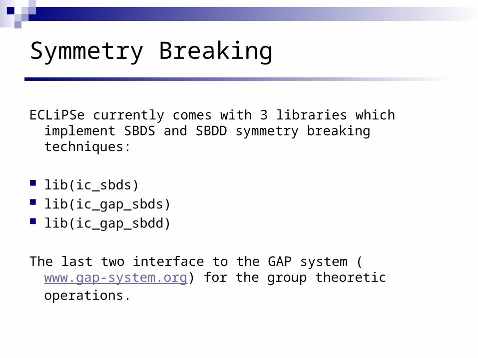
Symmetry Breakingwith lib(ic_sbds)
queens(Board) :-…sbds_initialise(Board, 2, [r90(Board, N), r180(Board, N), r270(Board, N), rx(Board, N), ry(Board, N), rd1(Board, N), rd2(Board, N)], #=, []),
search(Board, 0, input_order, sbds_indomain, sbds, []).
r90(Matrix, N, [I,J], Value, SymVar, SymValue) :- % 90 deg rotationSymVar is Matrix[J, N + 1 - I],SymValue is Value.
…rd2(Matrix, N, [I,J], Value, SymVar, SymValue) :- % d2 reflection SymVar is Matrix[N + 1 - J, N + 1 - I], SymValue is Value.

Symmetry Breakingwith lib(ic_gap_sbds)
queens(Board) :-. . .sbds_initialise(Board, [rows,cols], values:0..1,
[symmetry(s_n, [rows], []), symmetry(s_n, [cols], [])],[]),
search(Fields, 0, input_order, sbds_indomain, sbds, []).
Uses compact symmetry expressions [Harvey et al, SymCon, CP’03]
s_n index permutation in 1 dimensioncycle index rotation in 1 dimensionreverse index reversal in 1 dimensionr_4 rotation symmetry of the square in 2 dimensionsd_4 full symmetry of the square in 2 dimensionsgap_group(F)function(F)table(T)

Overview
How to model How to use solvers How to prototype constraints How to do tree search How to do optimization How to break symmetries How to do Local Search How to use LP/MIP How to do hybrids How to visualise

Tree SearchWith Local Search Flavour
E.g. Shuffle Searchtree search within subtrees
“local moves” between trees, preserving part of the previous solution’s variable assignments
Pesant & Gendreau, Neighbourhood Models

Tree Search with Local Search Flavour Restart with seeds, heuristics, limits
Jobshop example (approximation algorithm by Baptiste/LePape/Nuijten)
init_memory(Memory),bb_min((
( no_remembered_values(Memory) -> once bln_labeling(c, Resources, Tasks), % find a first solution remember_values(Memory, Resources, P); scale_down(P, PLimit, PFactor, Probability), % with decreasing
probability member(Heuristic, Heuristics), % try several heuristics repeat(N), % several times limit_backtracks(NB), % spending limited effort install_some_remembered_values(Memory, Resources, Probability), bb_min(
bln_labeling(Heuristic, Resources, Tasks),EndDate,bb_options{strategy:dichotomic}
), remember_values(Memory, Resources, Probability))
), EndDate, Tasks, TasksSol, EndApprox, bb_options{strategy:restart}).

Local Searchlib(tentative)
Tentative valuesX::1..5, X tent_set 3
In addition to other attributes (e.g. domain).Tentative value can be changed freely (unlike domain)Corresponds to incremental variables in Comet
Data-driven computation with tentative valuesSuspend until tentative value changes, then execute
ConstraintsMonitored for degree of violation, assuming tentative values
InvariantsZ tent_is X+Y
Update tentative value of Z whenever tentative value of X or Y changes (automatic and incremental)
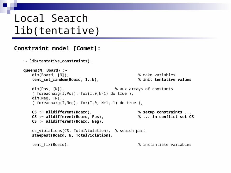
Local Searchlib(tentative)
Constraint model [Comet]:
:- lib(tentative_constraints).
queens(N, Board) :- dim(Board, [N]), % make variables tent_set_random(Board, 1..N), % init tentative values
dim(Pos, [N]), % aux arrays of constants ( foreacharg(I,Pos), for(I,0,N-1) do true ), dim(Neg, [N]), ( foreacharg(I,Neg), for(I,0,-N+1,-1) do true ),
CS :~ alldifferent(Board), % setup constraints ... CS :~ alldifferent(Board, Pos), % ... in conflict set CS CS :~ alldifferent(Board, Neg),
cs_violations(CS, TotalViolation), % search part steepest(Board, N, TotalViolation),
tent_fix(Board). % instantiate variables

Local Searchlib(tentative)
Search routine:
steepest(Board, N, Violations) :- vs_create(Board, Vars), % create variable set Violations tent_get V0, % initial violations SampleSize is fix(sqrt(N)), % neighbourhood size (
fromto(V0,_V1,V2,0), % until no violations left param(Vars,N,SampleSize,Violations)
do vs_worst(Vars, X), % get a most violated variable tent_minimize_random( % find a best neighbour ( % nondeterministic move generator random_sample(1..N,SampleSize,I), X tent_set I ), Violations, % violation variable I % best move-id ), X tent_set I, % do the move Violations tent_get V2 % new violations
).

Overview
How to model How to use solvers How to prototype constraints How to do tree search How to do optimization How to break symmetries How to do Local Search How to use LP/MIP How to do hybrids How to visualise

Mathematical ProgrammingSolving with Linear Programming
:- lib(eplex).
solve(Vars, Cost) :-model(Vars, Obj),eplex_solver_setup(min(Obj)),eplex_solve(Cost).
model(Vars, Obj) :-Vars = [A1, A2, A3, B1, B2, B3, C1, C2, C3, D1, D2, D3],Vars :: 0..inf,A1 + A2 + A3 $= 200,B1 + B2 + B3 $= 400,C1 + C2 + C3 $= 300,D1 + D2 + D3 $= 100,A1 + B1 + C1 + D1 $=< 500,A2 + B2 + C2 + D2 $=< 300,A3 + B3 + C3 + D3 $=< 400,Obj = 10*A1 + 7*A2 + 11*A3 + 8*B1 + 5*B2 + 10*B3 + 5*C1 + 5*C2 + 8*C3 + 9*D1 + 3*D2 + 7*D3.
500
300
400
200
100
400
300
10
89
75
11
5
35
108
7
Plantcapacity
Clientdemand
Transportationcost
A
B
C
D
1
2
3

Mathematical Programming Features of eplex
Support for: COIN/OSI, CPLEX, Xpress MP LP, MIP, QP, MIQP as supported by the solver Adding constraints and resolving problem (remove
constraints on backtracking) Data driven/event triggering of solver Encapsulated modifications of problem Multiple problem instances Options to solver, e.g. changing solving method,
presolve, time-outs… Support for column generation Cut pools

Mathematical Programming Encapsulated modifications: eplex_probe Allow problem to be modified temporarily and (re)solved
Change/perturb objective
Change variable bounds, RHS coefficients,
Relax integers constraints….
Modification is encapsulated into the probe predicate, e.g.What if the transportation cost from plant 1 to warehouse A is
increased from 10 to 20?….eplex_probe([perturb_obj([A1:10])], NewCost)
oreplex_probe([min(20*A1+7*A2+11*A3 ...)], NewCost)

Overview
How to model How to use solvers How to prototype constraints How to do tree search How to do optimization How to break symmetries How to use LP/MIP How to do LS How to do hybrids How to visualise

Solving a Problem with Multiple Solvers
Real problems comprise different subproblemsDifferent solvers/algorithms suit different subproblems
Global reasoning can be achieved in different waysLinear solvers reason globally on linear constraintsDomain solvers support application-specific global
constraints
Solvers complement each otherOptimisation versus feasibilityNew and adapted forms of cooperation
(e.g. Linear relaxation as a heuristic)

Co-operating Solvers in ECLiPSe
Modelling of different (sub)problems for different solvers can use the same logical variables: ic: (X #>= 3), eplex: (X + Y $=< 3.0)
Common Solver Interface – same syntax for constraints in different solvers ic: (X $=< 3), eplex: (Y $=< 3) [ic, eplex]: (X + Y $=:= Z + 3)Solver: (X+Y $>= 3)

Example: Bridge Scheduling Problem
Linear precedence + distance constraints (min/max time between tasks)
Non-linear resource usage constraints: nonoverlap of tasks using the same resource
Find optimal solution (minimise) Hybrid solution for problem using probe backtrack
search – note real problems that benefits from hybrid will be more complicated.

Ignore hard constraintsIn subproblem(nonoverlap)Monitor hard constraintsfor violation
Problem
Probe Backtrack Search
subproblem
Solve subproblem with probe(linear solver)
Conflicting constraintsfor main problem(monitored)
add constraint to subproblemto resolve one conflict(remove overlap)
resolve subproblem withadded constraintsMore than one way to resolve constraint ->search

Information transfer
ICFinite domain
Linear constraints
EPLEXContinuous
Linear constraints
TENTATIVENon-linear (monitored)
Subproblem solution valuesLinear precedence constraints
Variable bounds
Branch & BoundSearch

Bridge Probe Backtrack Example:- lib(tentative), lib(eplex),lib(ic),lib(branch_and_bound).:- local struct(task(start,duration,need,use)).go(End_date) :-
Tasks = [PA,….],PA = task{duration : 0, need : []},A1 = task{duration : 4, need : [PA], use : excavator},
….end_to_end_max(S6, B6, 4),
….end_to_start_max(A6, S6, 3),
….start_to_start_min(UE, Start_of_F, 6),end_to_start_min(End_of_M, UA, -2),tasks_starts(Tasks,Starts),ic:integers(Starts),(foreach(task{start:Si,duration:_Di,need:NeededTasks}, Tasks) do [ic,eplex]:(Si $>= 0),),
(foreach(task{start:Sj,duration:Dj},NeededTasks), param(Si) do[ic,eplex]:(Si $>= Sj+Dj) )
),tent_set_all(Starts, 0),disjunct_setup(Tasks, CS),eplex_solver_setup(min(End_date), End_date, [sync_bounds(yes)/]. new_constraint, deviating_bounds, post( post_eplex_solve )]),minimize((
repair_label(CS),tent_fix(Starts) ), End_date).
post_eplex_solve :- eplex_get(vars, Vs), eplex_get(typed_solution, Vals), ( foreacharg(V,Vs), foreacharg(Val0, Vals) do
Val is fix(round(Val0)), V tent_set Val ).
start_to_start_min(task{start:S1}, task{start:S2}, Min) :-[ic,eplex]:(S1+Min $=< S2).
end_to_end_max(task{start:S1,duration:D1}, task{start:S2,duration:D2}, Max) :-[ic,eplex]:(S1+D1+Max $>=S2+D2).
end_to_start_min(task{start:S1,duration:D1}, task{start:S2}, Min) :-[ic,eplex]:(S1+D1+Min $=< S2.
end_to_start_max(task{start:S1,duration:D1}, task{start:S2}, Max) :-[ic,eplex]:(S1+D1+Max $>= S2.
disjunct_setup(Tasks, CS) :-cs_create(CS, []),( fromto(Tasks, [Task0|Tasks0], Tasks0, []), param(CS) do ( foreach(Task1,Tasks0), param(Task0,CS) do Task0 = task{start:S0, duration:D0, use:R0}, Task1 = task{start:S1, duration:D1, use:R1}, ( R0 == R1 ->
CS :~ nonoverlap(S0,D0,S1,D1) alias tasks(Task0, Task1) ;
true ) ) ).
nonoverlap(Si,Di,Sj,_Dj) :-[ic,eplex]: (Sj $>= Si+Di).
nonoverlap(Si,_Di,Sj,Dj) :- [ic,eplex]: (Si $>= Sj+Dj).repair_label(CS) :-
( cs_all_worst(CS, [tasks(Task0, Task1)|_]) -> Task0 = task{start:S0, duration:D0}, Task1 = task{start:S1, duration:D1}, nonoverlap(S0,D0,S1,D1),
repair_label(CS); true % no overlaps).

Bridge Example code
Use ic and eplex, tentative and branch_and_bound libraries
Use task structure to represent tasks::- local struct(task(start,duration,need,use)).
Constraint set up, e.g. :start_to_start_min(task{start:S1}, task{start:S2} , Min) :-
[ic,eplex]:(S1+Min $=< S2).

Setup of nonoverlap conflict monitoring
cs_create(CS, []), ( fromto(Tasks, [Task0|Tasks0], Tasks0, []), param(CS) do
( foreach(Task1,Tasks0), param(Task0,CS) do Task0 = task{start:S0, duration:D0, use:R0}, Task1 = task{start:S1, duration:D1, use:R1}, ( R0 == R1 ->
% tasks uses same resource – monitor for overlapCS :~ nonoverlap(S0,D0,S1,D1) alias
tasks(Task0,Task1) ;
true )
))
Handle to a conflict set
Add constraint to conflict set: monitored version called to
check for violation
alias defines how monitored
constraint is returned

Setup of eplex probe
……..eplex_solver_setup(min(Endtask), Endtask,
[ sync_bounds(yes) ],[ new_constraint, deviating_bounds, post( post_eplex_solve ) ]
), …..
post_eplex_solve :- eplex_get(vars, Vs),eplex_get(typed_solution, Vals),( foreacharg(V,Vs), foreacharg(Val0, Vals) do Val is fix(round(Val0)), V tent_set Val ).
Update bounds before solveTrigger solver when new constraints are
added…and when bounds change to exclude
existing eplex solution
solutionUpdate tentative value with the eplex solution values (as integer values). Violation of monitored constraints is
checked for
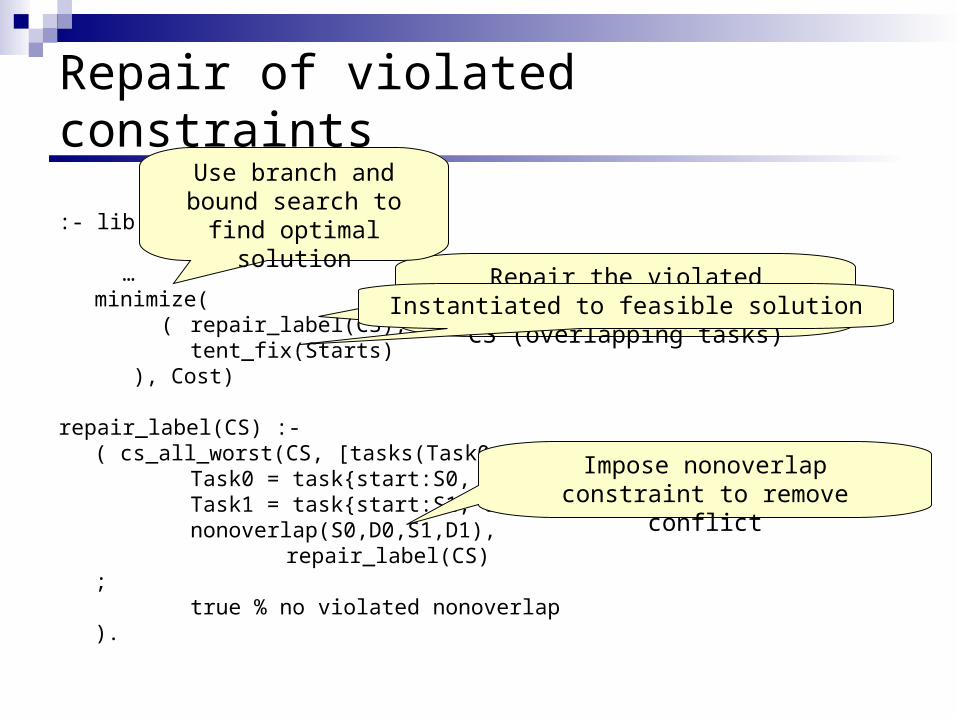
Repair of violated constraints
:- lib(branch_and_bound).
…minimize(
( repair_label(CS),tent_fix(Starts)
), Cost)
repair_label(CS) :-( cs_all_worst(CS, [tasks(Task0, Task1)|_]) ->
Task0 = task{start:S0, duration:D0}, Task1 = task{start:S1, duration:D1}, nonoverlap(S0,D0,S1,D1), repair_label(CS);
true % no violated nonoverlap).
Repair the violated constraint in constraint set CS (overlapping tasks)Instantiated to feasible solution
Use branch and bound search to find optimal
solution
Impose nonoverlap constraint to remove conflict
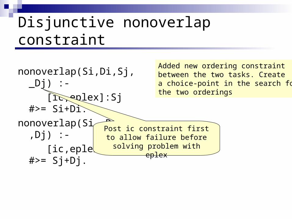
Disjunctive nonoverlap constraint
nonoverlap(Si,Di,Sj,_Dj) :- [ic,eplex]:Sj #>= Si+Di.
nonoverlap(Si,_Di,Sj,Dj) :- [ic,eplex]:Si #>= Sj+Dj.
Added new ordering constraintbetween the two tasks. Createa choice-point in the search forthe two orderings
Post ic constraint first to allow failure before solving problem with
eplex

Overview
How to model How to use solvers How to prototype constraints How to do tree search How to do optimization How to break symmetries How to use LP/MIP How to do LS How to do hybrids How to visualise

ToolsTkEclipse

ToolsTracer and Data Inspector

ToolsSaros – ECLiPSe/eclipse integration

ToolsVisualisation
:-lib(ic).:-lib(viewable).
sendmore1(Digits) :- Digits = [S,E,N,D,M,O,R,Y], Digits :: [0..9], viewable_create(equation, Digits), Carries = [C1,C2,C3,C4], Carries :: [0..1], alldifferent(Digits), S #\= 0, M #\= 0, C1 #= M, C2 + S + M #= O + 10*C1, C3 + E + O #= N + 10*C2, C4 + N + R #= E + 10*C3, D + E #= Y + 10*C4, lab(Carries), lab(Digits).

Tools Visualisation (arrays)

ToolsVisualisation (graphs)

Ongoing work
Evolve strengthsHigh level scripting and solver cooperationMore interfaces to good solvers (Gecode, MiniSat, …)
System EngineeringNew compilerRuntime improvements
Development EnvironmentSaros (ECLiPSe/eclipse)

Resources
BooksConstraint Logic Programming using ECLiPSe Krzysztof Apt & Mark Wallace, Cambridge University Press, 2006.
Programming with Constraints: an IntroductionKim Mariott & Peter Stuckey, MIT Press, 1998.
ECLiPSe is open-source (MPL)Main web site www.eclipse-clp.orgTutorial, papers, manuals, mailing listsSources at www.sourceforge.net/eclipse-clp