Embed Size (px)
Citation preview
Copyright © by Jose E. Schutt‐Aine , All Rights ReservedECE 598‐JS, Spring 2012 11
ECE 598 JS Lecture ‐09Scattering Parameters
Spring 2012
Jose E. Schutt-AineElectrical & Computer Engineering
University of [email protected]
Copyright © by Jose E. Schutt‐Aine , All Rights ReservedECE 598‐JS, Spring 2012 2
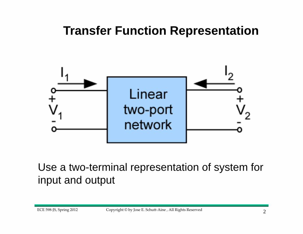
Transfer Function Representation
Use a two-terminal representation of system for input and output

Copyright © by Jose E. Schutt‐Aine , All Rights ReservedECE 598‐JS, Spring 2012 3
Y-parameter Representation
1 11 1 12 2
2 21 1 22 2
I y V y VI y V y V
= += +

Copyright © by Jose E. Schutt‐Aine , All Rights ReservedECE 598‐JS, Spring 2012 4
Y Parameter Calculations
2 2
1 211 21
1 10 0V V
I Iy yV V
= =
= =
To make V2= 0, place a short at port 2
Copyright © by Jose E. Schutt‐Aine , All Rights ReservedECE 598‐JS, Spring 2012 5
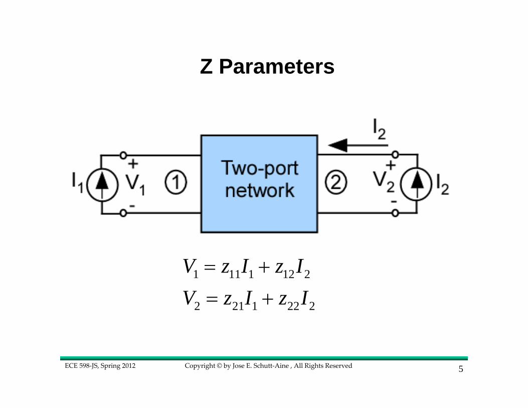
Z Parameters
1 11 1 12 2
2 21 1 22 2
V z I z IV z I z I
= += +
Copyright © by Jose E. Schutt‐Aine , All Rights ReservedECE 598‐JS, Spring 2012 6
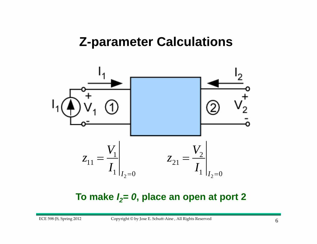
Z-parameter Calculations
2 2
1 211 21
1 10 0I I
V Vz zI I
= =
= =
To make I2= 0, place an open at port 2

Copyright © by Jose E. Schutt‐Aine , All Rights ReservedECE 598‐JS, Spring 2012 7
H Parameters
1 11 1 12 2
2 21 1 22 2
V h I h VI h I h V
= += +

Copyright © by Jose E. Schutt‐Aine , All Rights ReservedECE 598‐JS, Spring 2012 8
H Parameter Calculations
To make V2= 0, place a short at port 2
2 2
1 211 21
1 10 0V V
V Ih hI I
= =
= =

Copyright © by Jose E. Schutt‐Aine , All Rights ReservedECE 598‐JS, Spring 2012 9
G Parameters
1 11 1 12 2
2 21 1 22 2
I g V g IV g V g I
= += +

Copyright © by Jose E. Schutt‐Aine , All Rights ReservedECE 598‐JS, Spring 2012 10
G-Parameter Calculations
2 2
1 211 21
1 10 0I I
I Vg gV V
= =
= =
To make I2= 0, place an open at port 2

Copyright © by Jose E. Schutt‐Aine , All Rights ReservedECE 598‐JS, Spring 2012 1111
TWO‐PORT NETWORK REPRESENTATION
- At microwave frequencies, it is more difficult to measure total voltagesand currents.
- Short and open circuits are difficult to achieve at high frequencies.
- Most active devices are not short- or open-circuit stable.
1 11 1 12 2V Z I Z I= +
2 21 1 22 2V Z I Z I= +1 11 1 12 2I Y V Y V= +
2 21 1 22 2I Y V Y V= +
Z Parameters Y Parameters

Copyright © by Jose E. Schutt‐Aine , All Rights ReservedECE 598‐JS, Spring 2012 1212
1 11I = i r
o
E EZ− 2 2
2I = i r
o
E EZ−
- Total voltage and current are made up of sums of forward andbackward traveling waves.
- Traveling waves can be determined from standing-wave ratio.
Use a travelling wave approach
Wave Approach
1 1 1i rV E E= + 2 2 2i rV E E= +

Copyright © by Jose E. Schutt‐Aine , All Rights ReservedECE 598‐JS, Spring 2012 1313
11a = i
o
EZ
22a = i
o
EZ
11b = r
o
EZ
22b = r
o
EZ
Zo is the reference impedance of the system
b1 = S11 a1 + S12 a2
b2 = S21 a1 + S22 a2
Wave Approach
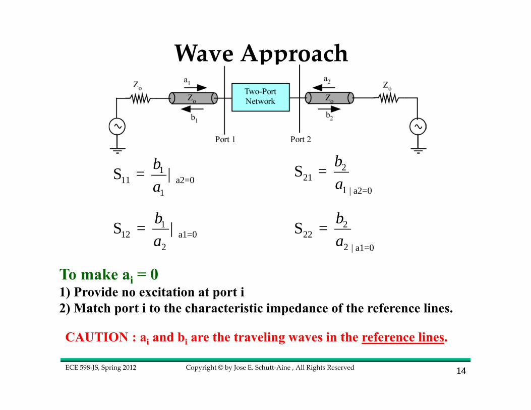
Copyright © by Jose E. Schutt‐Aine , All Rights ReservedECE 598‐JS, Spring 2012 1414
111 a2=0
1
S = | ba
221
1 | a2=0
S = ba
112 a1=0
2
S = | ba
222
2 | a1=0
S = ba
To make ai = 01) Provide no excitation at port i2) Match port i to the characteristic impedance of the reference lines.
CAUTION : ai and bi are the traveling waves in the reference lines.
Wave Approach

Copyright © by Jose E. Schutt‐Aine , All Rights ReservedECE 598‐JS, Spring 2012 1515
2
2 2
1111 22( X )S = S =
XΓ
Γ−−
2
2 2
1112 21( )XS = S =
XΓ
Γ−−
c ref
c ref
Z ZZ Z
Γ−
=+
( )( )R j L G j Cγ ω ω= + +
cR j LZG j C
ωω
+=
+
S‐Parameters of TL
lX e γ−=

Copyright © by Jose E. Schutt‐Aine , All Rights ReservedECE 598‐JS, Spring 2012 1616
2
2 2
1111 22( X )S = S =
XΓ
Γ−−
2
2 2
1112 21( )XS = S =
XΓ
Γ−−
c ref
c ref
Z ZZ Z
Γ−
=+
LCβ ω=
cLZC
=
S‐Parameters of Lossless TL
j lX e β−=
If Zc = Zref
011 22S = S = j l
12 21S = S = e β−

Copyright © by Jose E. Schutt‐Aine , All Rights ReservedECE 598‐JS, Spring 2012 17
N-Port S Parameters
1 11 12 1
2 21 22 2
n nn n
b S S ab S S a
b S a
⋅ ⋅⎡ ⎤ ⎡ ⎤ ⎡ ⎤⎢ ⎥ ⎢ ⎥ ⎢ ⎥⋅ ⋅⎢ ⎥ ⎢ ⎥ ⎢ ⎥=
⋅ ⋅ ⋅ ⋅ ⋅ ⋅⎢ ⎥ ⎢ ⎥ ⎢ ⎥⎢ ⎥ ⎢ ⎥ ⎢ ⎥⋅ ⋅ ⋅⎣ ⎦ ⎣ ⎦ ⎣ ⎦
b = Sa
ii
oi
VaZ
+
=
If bi = 0, then no reflected wave on port i port is matched
ii
oi
VbZ
−
=
iV +
iV −
oiZ
: incident voltage wave in port i
: reflected voltage wave in port i
: impedance in port i

Copyright © by Jose E. Schutt‐Aine , All Rights ReservedECE 598‐JS, Spring 2012 18
N-Port S Parameters
( ) ( )1o
o
ZZ
=a + b Z a - b
v = Zi( )1
oZ=i a - b
Substitute (1) and (2) into (3)
Defining S such that b = Sa and substituting for b( ) ( )
o oZ Z=U + S a U - S a
( )( ) 1oZ −=Z U + S U - S ( ) ( )o oZ Z= −-1S Z + U Z U
S Z Z S
(3)(2)(1)( )oZ=v a + b
U : unit matrix

Copyright © by Jose E. Schutt‐Aine , All Rights ReservedECE 598‐JS, Spring 2012 19
N-Port S Parameters
( )-1i = k a - b
If the port reference impedances are different, we define k as
v = k(a + b)
1
2
o
o
on
Z
Z
Z
⎡ ⎤⎢ ⎥⎢ ⎥= ⎢ ⎥⋅⎢ ⎥⎢ ⎥⎣ ⎦
k
( )= -1k(a + b) Zk a - b
( )( )-1Z = k U + S U - S k( )( )-1 -1S = Zk + k Zk - k
S ZZ S
and and
Copyright © by Jose E. Schutt‐Aine , All Rights ReservedECE 598‐JS, Spring 2012 20
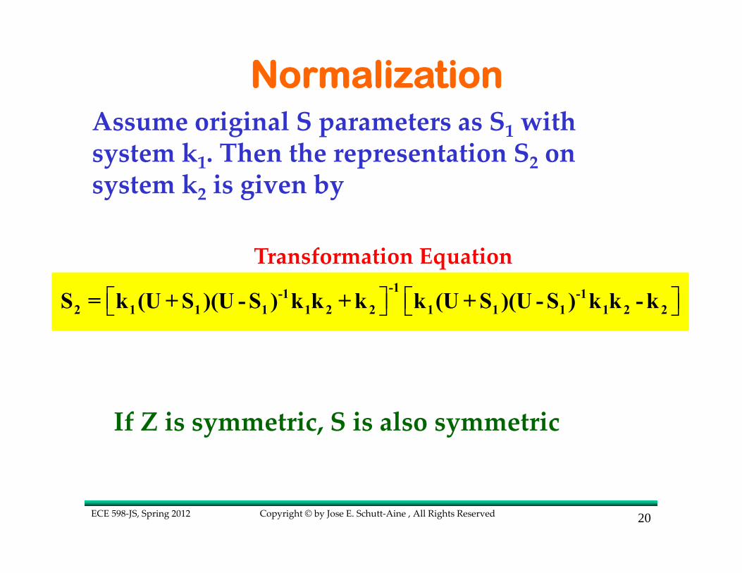
NormalizationAssume original S parameters as S1 with system k1. Then the representation S2 on system k2 is given by
⎡ ⎤ ⎡ ⎤⎣ ⎦ ⎣ ⎦-1-1 -1
2 1 1 1 1 2 2 1 1 1 1 2 2S = k (U + S )(U - S ) k k + k k (U + S )(U - S ) k k - k
Transformation Equation
If Z is symmetric, S is also symmetric
Copyright © by Jose E. Schutt‐Aine , All Rights ReservedECE 598‐JS, Spring 2012 21
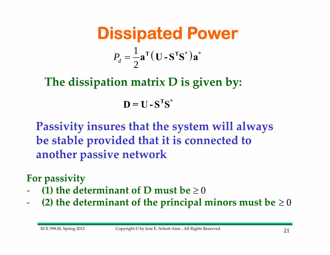
Dissipated Power( )1
2dP = T T * *a U - S S a
The dissipation matrix D is given by:T *D = U - S S
Passivity insures that the system will always be stable provided that it is connected to another passive network
For passivity‐ (1) the determinant of D must be‐ (2) the determinant of the principal minors must be
0≥0≥

Copyright © by Jose E. Schutt‐Aine , All Rights ReservedECE 598‐JS, Spring 2012 22
Dissipated Power
=T *S S U
When the dissipation matrix is 0, we have a lossless network
The S matrix is unitary.
2 211 21 1S S+ =
2 222 12 1S S+ =
For a lossless two‐port:
If in addition the network is reciprocal, then2
12 21 11 22 12and 1S S S S S= = = −
Copyright © by Jose E. Schutt‐Aine , All Rights ReservedECE 598‐JS, Spring 2012 23
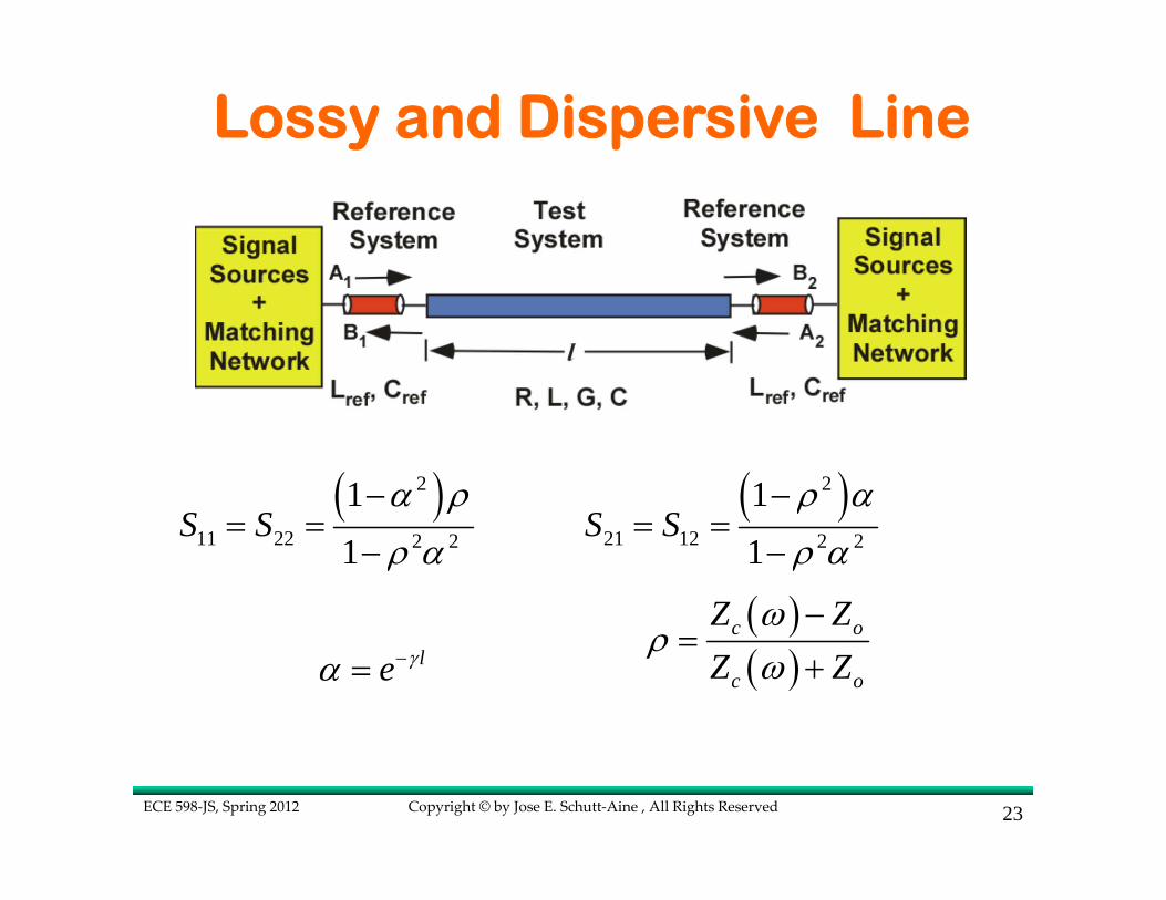
Lossy and Dispersive Line
( )2
11 22 2 2
11
S S−
= =−
α ρ
ρ α( )2
21 12 2 2
11
S S−
= =−
ρ α
ρ α
le−= γα( )( )
c o
c o
Z ZZ Z
−=
+ω
ρω

Copyright © by Jose E. Schutt‐Aine , All Rights ReservedECE 598‐JS, Spring 2012 24
Frequency-Domain Formulation*
* J. E. Schutt-Aine and R. Mittra, "Scattering Parameter Transient analysis of transmission lines loaded with nonlinear terminations," IEEE Trans. Microwave Theory Tech., vol. MTT-36, pp. 529-536, March 1988.

Copyright © by Jose E. Schutt‐Aine , All Rights ReservedECE 598‐JS, Spring 2012 25
( ) ( )1 11 1 12 2( ) ( ) ( )B S A S A= +ω ω ω ω ω
( ) ( )2 21 1 22 2( ) ( ) ( )B S A S A= +ω ω ω ω ω
Frequency-Domain

Copyright © by Jose E. Schutt‐Aine , All Rights ReservedECE 598‐JS, Spring 2012 26
Time-Domain Formulation

Copyright © by Jose E. Schutt‐Aine , All Rights ReservedECE 598‐JS, Spring 2012 27
Time-Domain Formulation
1 11 1 12 2( ) ( )* ( ) ( )* ( )b t s t a t s t a t= +
2 21 1 22 2( ) ( )* ( ) ( )* ( )b t s t a t s t a t= +
1 1 1 1 1( ) ( ) ( ) ( ) ( )a t t b t T t g t= Γ +
2 2 2 2 2( ) ( ) ( ) ( ) ( )a t t b t T t g t= Γ +
( )( )
oi
i o
ZT tZ t Z
=+
( )( )( )
i oi
i o
Z t ZtZ t Z
−Γ =
+

Copyright © by Jose E. Schutt‐Aine , All Rights ReservedECE 598‐JS, Spring 2012 28
Time-Domain Solutions
[ ]'2 22 1 1 1 1
1
1 ( ) (0) ( ) ( ) ( ) ( )( )
( )t s T t g t t M t
a tt
⎡ ⎤− Γ + Γ⎣ ⎦=Δ
[ ]'1 12 2 2 2 2( ) (0) ( ) ( ) ( ) ( )
( )t s T t g t t M t
t
⎡ ⎤Γ + Γ⎣ ⎦+Δ
[ ]'1 11 2 2 2 2
2
1 ( ) (0) ( ) ( ) ( ) ( )( )
( )t s T t g t t M t
a tt
⎡ ⎤− Γ + Γ⎣ ⎦=Δ
[ ]'2 21 1 1 1 1( ) (0) ( ) ( ) ( ) ( )
( )t s T t g t t M t
t
⎡ ⎤Γ + Γ⎣ ⎦+Δ

Copyright © by Jose E. Schutt‐Aine , All Rights ReservedECE 598‐JS, Spring 2012 29
Time-Domain Solutions
' ' ' '1 11 2 22 1 12 2 21( ) 1 ( ) (0) 1 ( ) (0) ( ) (0) ( ) (0)t t s t s t s t s⎡ ⎤ ⎡ ⎤Δ = − Γ − Γ − Γ Γ⎣ ⎦ ⎣ ⎦
' (0) (0)ij ijs s= Δτ
1 11 12( ) ( ) ( )M t H t H t= +
2 21 22( ) ( ) ( )M t H t H t= +
1
1
( ) ( ) ( )t
ij ij jH t s t a−
=
= − Δ∑τ
τ τ τ
' '1 11 1 12 2 1( ) (0) ( ) (0) ( ) ( )b t s a t s a t M t= + +
' '2 21 1 22 2 2( ) (0) ( ) (0) ( ) ( )b t s a t s a t M t= + +

Copyright © by Jose E. Schutt‐Aine , All Rights ReservedECE 598‐JS, Spring 2012 30
Special Case – Lossless Line
11 22( ) ( ) 0s t s t= = 12 21( ) ( ) ls t s t tv
⎛ ⎞= = −⎜ ⎟⎝ ⎠
δ
1 2( ) lM t a tv
⎛ ⎞= −⎜ ⎟⎝ ⎠
2 1( ) lM t a tv
⎛ ⎞= −⎜ ⎟⎝ ⎠
( )1 1 1 1 2( ) ( ) ( ) la t T t g t t a tv
⎛ ⎞= + Γ −⎜ ⎟⎝ ⎠
( )2 2 2 2 1( ) ( ) ( ) la t T t g t t a tv
⎛ ⎞= + Γ −⎜ ⎟⎝ ⎠
1 2( ) lb t a tv
⎛ ⎞= −⎜ ⎟⎝ ⎠
2 1( ) lb t a tv
⎛ ⎞= −⎜ ⎟⎝ ⎠
Wave Shifting Solution

Copyright © by Jose E. Schutt‐Aine , All Rights ReservedECE 598‐JS, Spring 2012 31
Time-Domain Solutions
1 1 1( ) ( ) ( )v t a t b t= +
2 2 2( ) ( ) ( )v t a t b t= +
1 11
( ) ( )( )o o
a t b ti tZ Z
= −
2 22
( ) ( )( )o o
a t b ti tZ Z
= −
Copyright © by Jose E. Schutt‐Aine , All Rights ReservedECE 598‐JS, Spring 2012 32
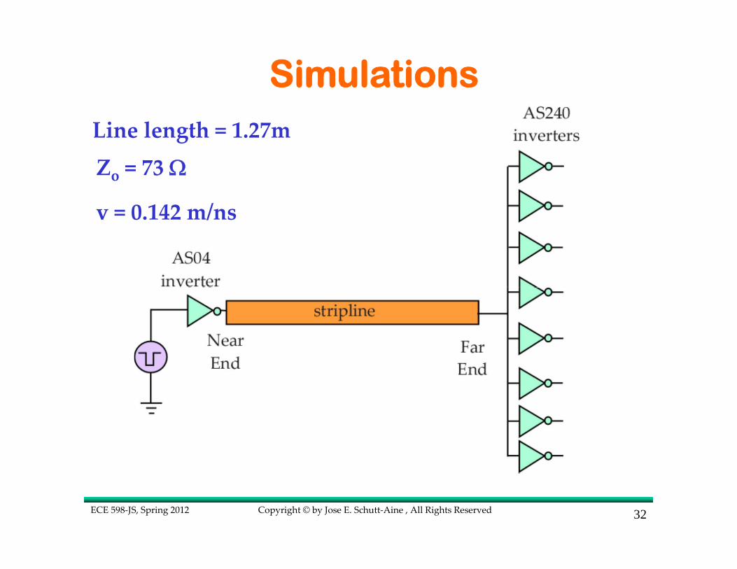
SimulationsLine length = 1.27mZo = 73 Ω
v = 0.142 m/ns
Copyright © by Jose E. Schutt‐Aine , All Rights ReservedECE 598‐JS, Spring 2012 33
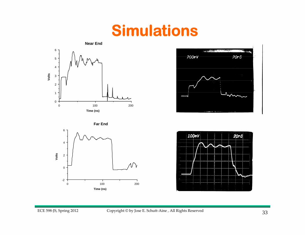
0 100 2000
1
2
3
4
5
6
Near End
Time (ns)
Volts
0 100 200-2
0
2
4
6
Far End
Time (ns)
Volts
Simulations

Copyright © by Jose E. Schutt‐Aine , All Rights ReservedECE 598‐JS, Spring 2012 34
0 10 20 30 40 50-1
0
1
2
3
4
5
lossylossless
Near End
Time (ns)
Volts
0 10 20 30 40 50-2
0
2
4
6
lossylossless
Far End
Time (ns)
Volts
Simulations
Line length = 25 in
L = 539 nH/m
C = 39 pF/m
Ro = 1 kΩ (GHz)1/2
Pulse magnitude = 4V
Pulse width = 20 ns
Rise and fall times = 1ns
Copyright © by Jose E. Schutt‐Aine , All Rights ReservedECE 598‐JS, Spring 2012 35
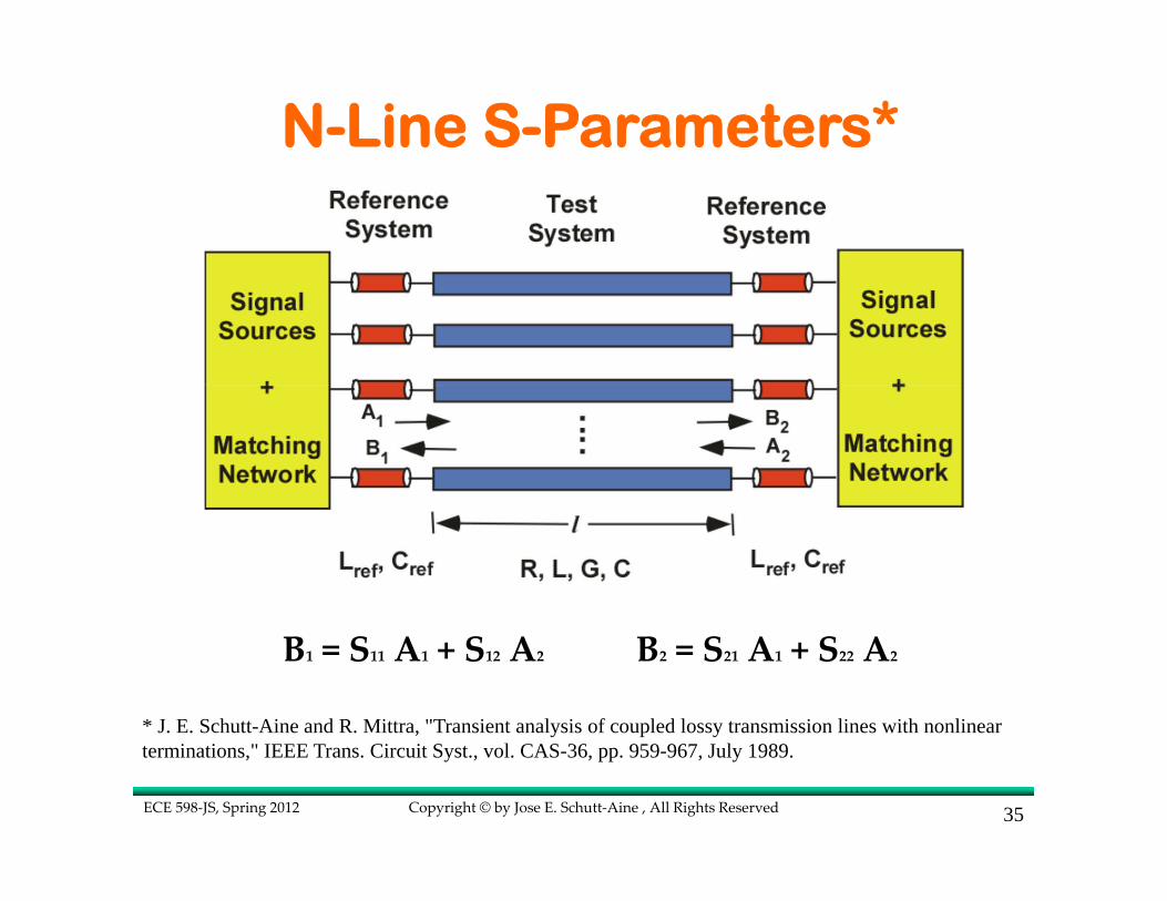
N-Line S-Parameters*
B1 = S11 A1 + S12 A2 B2 = S21 A1 + S22 A2
* J. E. Schutt-Aine and R. Mittra, "Transient analysis of coupled lossy transmission lines with nonlinear terminations," IEEE Trans. Circuit Syst., vol. CAS-36, pp. 959-967, July 1989.
Copyright © by Jose E. Schutt‐Aine , All Rights ReservedECE 598‐JS, Spring 2012 36
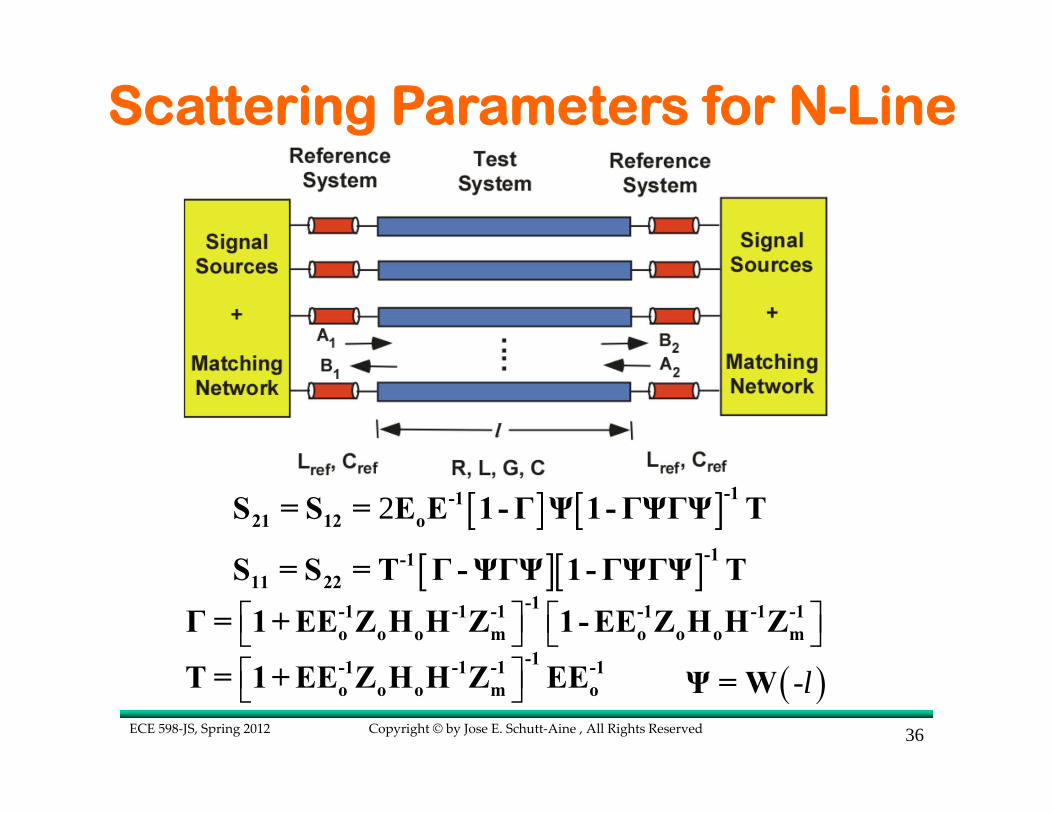
Scattering Parameters for N-Line
[ ][ ]-1-111 22S = S = T Γ -ΨΓΨ 1-ΓΨΓΨ T
[ ] [ ]2 -1-121 12 oS = S = E E 1-Γ Ψ 1-ΓΨΓΨ T
⎡ ⎤ ⎡ ⎤⎣ ⎦ ⎣ ⎦-1-1 -1 -1 -1 -1 -1
o o o m o o o mΓ = 1+ EE Z H H Z 1- EE Z H H Z
⎡ ⎤⎣ ⎦-1-1 -1 -1 -1
o o o m oT = 1+ EE Z H H Z EE ( )-lΨ = W
Copyright © by Jose E. Schutt‐Aine , All Rights ReservedECE 598‐JS, Spring 2012 37
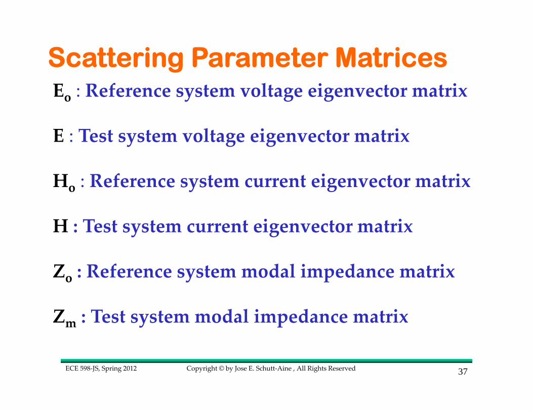
Scattering Parameter MatricesEo : Reference system voltage eigenvector matrix
E : Test system voltage eigenvector matrix
Ho : Reference system current eigenvector matrix
H : Test system current eigenvector matrix
Zo : Reference system modal impedance matrix
Zm : Test system modal impedance matrix

Copyright © by Jose E. Schutt‐Aine , All Rights ReservedECE 598‐JS, Spring 2012 38
Eigen Analysis
* Diagonalize ZY and YZ and find eigenvalues.* Eigenvalues are complex: λi = αi + jβi
W(u) =
eα1u+ jβ1u
eα2u+ jβ2u
•eαn u+ jβnu
⎡
⎣
⎢ ⎢ ⎢ ⎢ ⎢
⎤
⎦
⎥ ⎥ ⎥ ⎥ ⎥

Copyright © by Jose E. Schutt‐Aine , All Rights ReservedECE 598‐JS, Spring 2012 39
Solution
mV = EV
mI = HI
[ ]( ) ( ) ( )x x x− + ΒmV = W A W
[ ]( ) ( ) ( )x x x− + Β-1m mI = Z W A W
-1 -1m mZ = Λ EZH
-1 -1 -1c m mZ = E Z H = E Λ EZ
Copyright © by Jose E. Schutt‐Aine , All Rights ReservedECE 598‐JS, Spring 2012 40
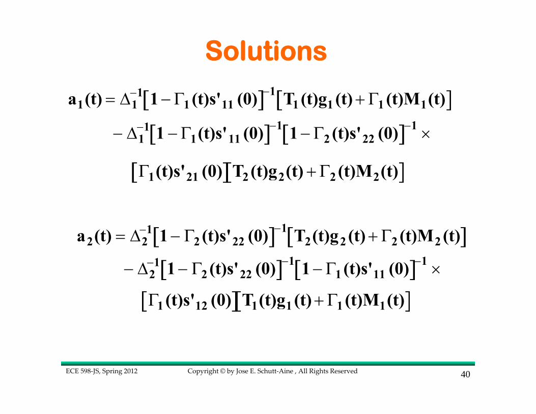
Solutions
a1(t) = Δ1−1 1 − Γ1 (t)s'11 (0)[ ]−1 T1 (t)g1 (t) + Γ1 (t)M1(t)[ ]
− Δ1−1 1 − Γ1(t)s'11 (0)[ ]−1 1 − Γ2 (t)s'22 (0)[ ]−1 ×
Γ1(t)s'21 (0)[ ]T2 (t)g2(t) + Γ2 (t)M2(t)[ ]
a2(t) = Δ2−1 1 − Γ2 (t)s'22 (0)[ ]−1 T2(t)g2 (t) + Γ2 (t)M2 (t)[ ]
− Δ2−1 1 − Γ2 (t)s'22 (0)[ ]−1 1 − Γ1 (t)s'11 (0)[ ]−1 ×
Γ1 (t)s'12 (0)[ ] T1(t)g1 (t) + Γ1 (t)M1(t)[ ]
Copyright © by Jose E. Schutt‐Aine , All Rights ReservedECE 598‐JS, Spring 2012 41
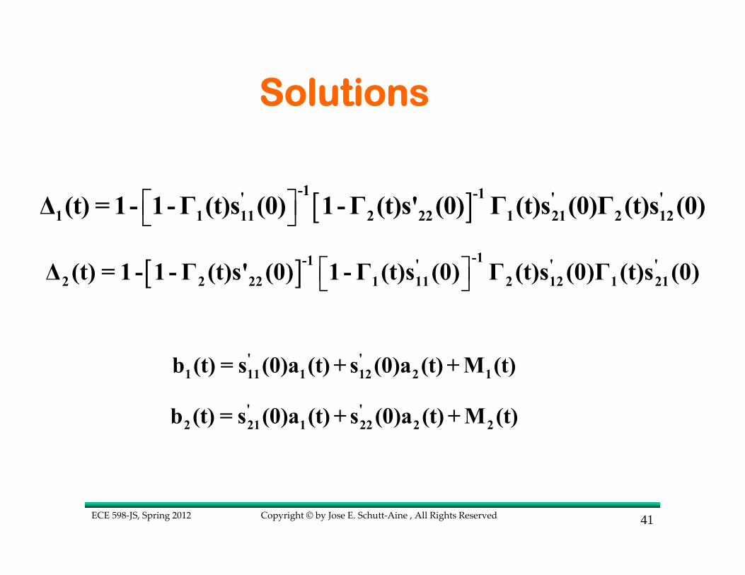
Solutions
[ ]⎡ ⎤⎣ ⎦-1 -1' ' '
1 1 11 2 22 1 21 2 12Δ (t) = 1- 1-Γ (t)s (0) 1-Γ (t)s' (0) Γ (t)s (0)Γ (t)s (0)
[ ] ⎡ ⎤⎣ ⎦-1-1 ' ' '
2 2 22 1 11 2 12 1 21Δ (t) = 1 - 1 -Γ (t)s' (0) 1 -Γ (t)s (0) Γ (t)s (0)Γ (t)s (0)
' '2 21 1 22 2 2b (t) = s (0)a (t) + s (0)a (t) + M (t)
' '1 11 1 12 2 1b (t) = s (0)a (t) + s (0)a (t) + M (t)
Copyright © by Jose E. Schutt‐Aine , All Rights ReservedECE 598‐JS, Spring 2012 42
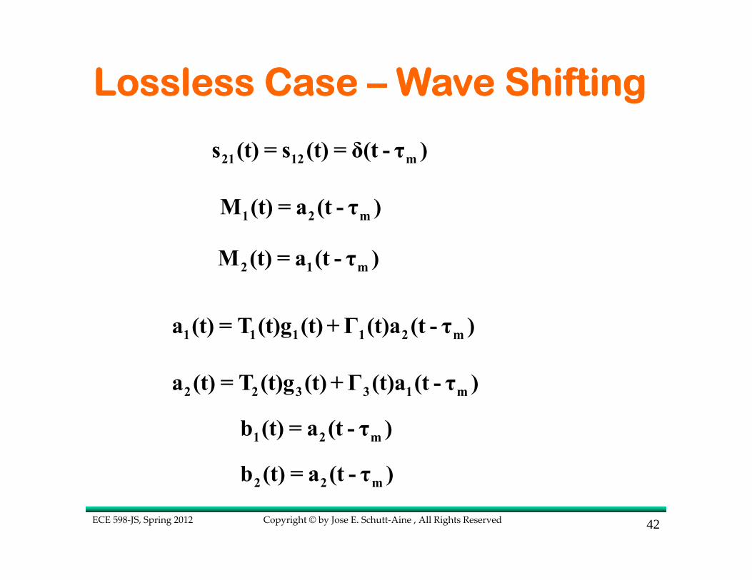
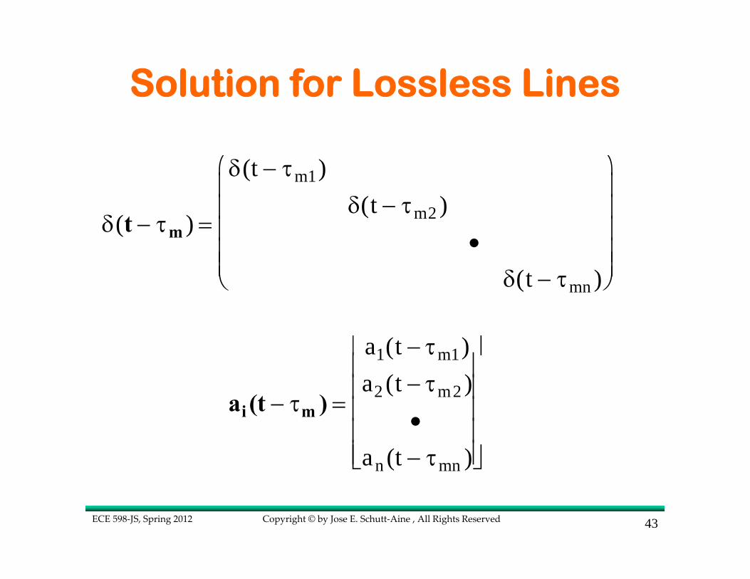
Lossless Case – Wave Shifting
21 12 ms (t) = s (t) = δ(t - τ )
1 2 mM (t) = a (t - τ )
2 1 mM (t) = a (t - τ )
1 1 1 1 2 ma (t) = T (t)g (t) +Γ (t)a (t - τ )
2 2 3 3 1 ma (t) = T (t)g (t) +Γ (t)a (t - τ )
1 2 mb (t) = a (t - τ )
2 2 mb (t) = a (t - τ )
Copyright © by Jose E. Schutt‐Aine , All Rights ReservedECE 598‐JS, Spring 2012 43
δ(t − τm ) =
δ(t − τm1)δ(t − τm2 )
•δ(t − τmn )
⎛
⎝
⎜ ⎜ ⎜ ⎜ ⎜
⎞
⎠
⎟ ⎟ ⎟ ⎟ ⎟
ai (t − τm ) =
a1(t − τm1)a2 (t − τm2 )
•an (t − τmn )
⎡
⎣
⎢ ⎢ ⎢ ⎢ ⎢
⎤
⎦
⎥ ⎥ ⎥ ⎥ ⎥
Solution for Lossless Lines
Copyright © by Jose E. Schutt‐Aine , All Rights ReservedECE 598‐JS, Spring 2012 44
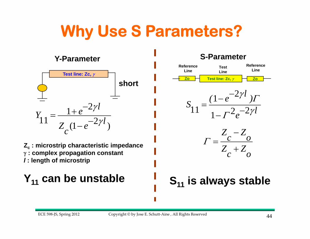
2111 2(1 )
leY lZ ec
γγ
−+=−−
Zc : microstrip characteristic impedanceγ : complex propagation constantl : length of microstrip
Y11 can be unstable
2111 221
l( e )S le
γ ΓγΓ
−−=
−−
Z Zc oZ Zc o
Γ−
=+
S11 is always stable
Y-Parameter S-Parameter
Test line: Zc, γ
shortZoZo
ReferenceLine
ReferenceLine
Test line: Zc, γ
TestLine
Why Use S Parameters?

Copyright © by Jose E. Schutt‐Aine , All Rights ReservedECE 598‐JS, Spring 2012 45
c ref
c ref
Z ZZ Z
−Γ =
+ cR j LZG j C
ωω
+=
+
Zref is arbitraryWhat is the best choice for Zref ?
refLZC
=
cLZC
→
11 0S →12j LCd
oS e Xω−→ =
At high frequencies
Thus, if we choose
Choice of Reference

Copyright © by Jose E. Schutt‐Aine , All Rights ReservedECE 598‐JS, Spring 2012 46
50.0 0.0 0.0 0.00.0 50.0 0.0 0.00.0 0.0 50.0 0.00.0 0.0 0.0 50.0
S-Parameter measurements (or simulations) aremade using a 50-ohm system. For a 4-port, the reference impedance is given by:
Zo =
11 1o oS ZZ I ZZ I
−− −⎡ ⎤ ⎡ ⎤= + −⎣ ⎦ ⎣ ⎦
[ ][ ] 1oZ I S I S Z−= + −
Z: Impedance matrix (of blackbox)S: S-parameter matrixZo: Reference impedanceI: Unit matrix
Choice of Reference

Copyright © by Jose E. Schutt‐Aine , All Rights ReservedECE 598‐JS, Spring 2012 47
328.0 69.6 328.9 69.669.6 328.8 69.6 328.9328.9 69.6 328.8 69.669.6 328.9 69.6 328.8
50.0 0.0 0.0 0.00.0 50.0 0.0 0.00.0 0.0 50.0 0.00.0 0.0 0.0 50.0
Method: Change reference impedance from uncoupled to coupled system to get new S-parameter representation
Zo =
Zo =
Uncoupled system
Coupled system
as an example…
Reference Transformation

Copyright © by Jose E. Schutt‐Aine , All Rights ReservedECE 598‐JS, Spring 2012 48
0
0.5
1
1.5
0 2 4 6 8 10
S11 - Linear Magnitude
S11 - 50 Ohm
S11 - Zref
S11
Frequency (GHz)
50.0 0.0 0.0 0.00.0 50.0 0.0 0.00.0 0.0 50.0 0.00.0 0.0 0.0 50.0
using
Zo =
as reference…
328.0 69.6 328.9 69.669.6 328.8 69.6 328.9328.9 69.6 328.8 69.669.6 328.9 69.6 328.8
using
as reference…
Zo =
Harder toapproximate
Easier to approximate (up to 6 GHz)
Choice of Reference

Copyright © by Jose E. Schutt‐Aine , All Rights ReservedECE 598‐JS, Spring 2012 49
0
0.5
1
1.5
0 2 4 6 8 10
S11 - Linear Magnitude
S11 - 50 Ohm
S11 - Zref
S11
Frequency (GHz)
50.0 0.0 0.0 0.00.0 50.0 0.0 0.00.0 0.0 50.0 0.00.0 0.0 0.0 50.0
using
Zo =
as reference…
328.0 69.6 328.9 69.669.6 328.8 69.6 328.9328.9 69.6 328.8 69.669.6 328.9 69.6 328.8
using
as reference…
Zo =
Harder toapproximate
Easier to approximate (up to 6 GHz)
Choice of Reference

Copyright © by Jose E. Schutt‐Aine , All Rights ReservedECE 598‐JS, Spring 2012 50
0
0.05
0.1
0.15
0.2
0.25
0.3
0 2 4 6 8 10
S12 - Linear Magnitude
S12 - 50 Ohm
S12 - Zref
S12
Frequency (GHz)
50.0 0.0 0.0 0.00.0 50.0 0.0 0.00.0 0.0 50.0 0.00.0 0.0 0.0 50.0
using
Zo =
as reference…
328.0 69.6 328.9 69.669.6 328.8 69.6 328.9328.9 69.6 328.8 69.669.6 328.9 69.6 328.8
using
as reference…
Zo =
Easier to approximate (up to 6 GHz)
Harder toapproximate
Choice of Reference

Copyright © by Jose E. Schutt‐Aine , All Rights ReservedECE 598‐JS, Spring 2012 51
0
0.2
0.4
0.6
0.8
1
1.2
0 2 4 6 8 10
S31 - Linear Magnitude
S31 - 50 Ohm
S31 - ZrefS3
1
Frequency (GHz)
50.0 0.0 0.0 0.00.0 50.0 0.0 0.00.0 0.0 50.0 0.00.0 0.0 0.0 50.0
using
Zo =
as reference…
328.0 69.6 328.9 69.669.6 328.8 69.6 328.9328.9 69.6 328.8 69.669.6 328.9 69.6 328.8
using
as reference…
Zo =
Harder toapproximate
Easier to approximate
Choice of Reference

Copyright © by Jose E. Schutt‐Aine , All Rights ReservedECE 598‐JS, Spring 2012 52
.
0
0.05
0.1
0.15
0.2
0.25
0.3
0 0.5 1 1.5 2 2.5 3
S11 Magnitude
Zref=ZoZref=80 ohmsZref=100 ohms
Frequency (GHz)
S11
Choice of Reference

Copyright © by Jose E. Schutt‐Aine , All Rights ReservedECE 598‐JS, Spring 2012 53
.
0.7
0.75
0.8
0.85
0 0.5 1 1.5 2 2.5 3
S21 Magnitude
Zref=ZoZref=80 ohmsZref=100 ohms
Frequency (GHz)
S21
Choice of Reference
Copyright © by Jose E. Schutt‐Aine , All Rights ReservedECE 598‐JS, Spring 2012 54
Modeling of Discontinuities
1. Tapered Lines
2. Capacitive Discontinuities

Copyright © by Jose E. Schutt‐Aine , All Rights ReservedECE 598‐JS, Spring 2012 55
General topology of tapered microstrip with dw :width at wide end,dn: width at narrow end, lw: length of wide section, ln : length ofnarrow section, lt: length of tapered section.
Tapered Microstrip

Copyright © by Jose E. Schutt‐Aine , All Rights ReservedECE 598‐JS, Spring 2012 56
( ) ( )21 1 22( ) ( )* ( ) ( )* ( )j j
j j ju t s t u t s t w t−= +
( 1) ( 1)11 12 1( ) ( )* ( ) ( )* ( )j j
j j jw t s t u t s t w t+ ++= +
* J. E. Schutt-Aine, IEEE Trans. Circuit Syst., vol. CAS-39, pp. 378-385, May 1992.
Tapered Line Analysis Using S Parameters*

Copyright © by Jose E. Schutt‐Aine , All Rights ReservedECE 598‐JS, Spring 2012 57
-1
0
1
2
3
4
5
0 1 2 3 4 5 6
Vol
ts
Time (ns)
Small EndExcitation at small end
-1
0
1
2
3
4
5
0 1 2 3 4 5 6
Vol
ts
Time (ns)
Wide EndExcitation at small end
-1
0
1
2
3
4
5
0 1 2 3 4 5 6
Vol
ts
Time (ns)
Small EndExcitation at wide end
-1
0
1
2
3
4
5
0 1 2 3 4 5 6
Vol
ts
Time (ns)
Wide EndExcitation at wide end
Tapered Transmission Line

Copyright © by Jose E. Schutt‐Aine , All Rights ReservedECE 598‐JS, Spring 2012 58
-1
0
1
2
3
4
5
0 1 2 3 4 5Time (ns)
Near End
.0564 mils/in
.1128 mils/in
.2257 mils/in
6 7 8
volts
-1
0
1
2
3
4
5
0 1 2 3 4 5Time (ns)
Far End
.0564 mils/in
.1128 mils/in
.2257 mils/in
6 7 8
volts
Varying tapering rate
Tapered Transmission Line

Copyright © by Jose E. Schutt‐Aine , All Rights ReservedECE 598‐JS, Spring 2012 59
Zo
Zo
ZoC
-1
-0.5
0
0.5
1
1.5
2
2.5
0 10 20 30 40 50
Near End -- C=4 pF
Vol
ts
Time (ns)
-1
-0.5
0
0.5
1
1.5
2
2.5
0 10 20 30 40 50
Far end -- C=4 pF
Vol
ts
Time (ns)
Capacitive Load

Copyright © by Jose E. Schutt‐Aine , All Rights ReservedECE 598‐JS, Spring 2012 60
Zo
Zo
ZoC
-1
-0.5
0
0.5
1
1.5
2
2.5
0 10 20 30 40 50
Near end -- C=40 pF
Vol
ts
Time (ns)
-0.5
0
0.5
1
1.5
2
2.5
0 10 20 30 40 50
Far end -- C=40 pF
Vol
ts
Time (ns)
Capacitive Load
Copyright © by Jose E. Schutt‐Aine , All Rights ReservedECE 598‐JS, Spring 2012 61
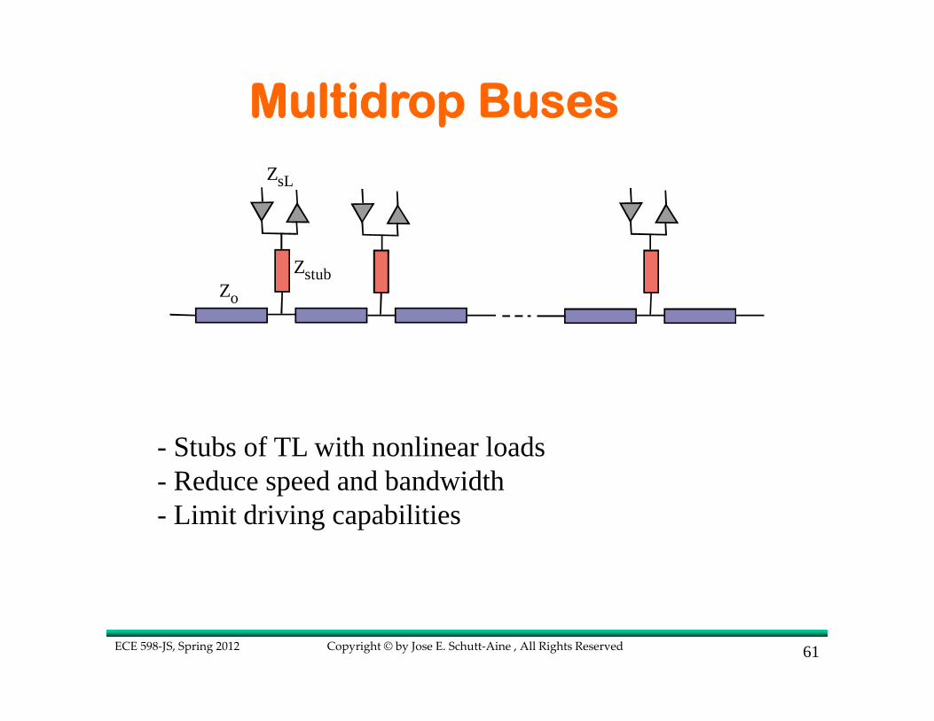
Zo
Zstub
ZsL
- Stubs of TL with nonlinear loads- Reduce speed and bandwidth - Limit driving capabilities
Multidrop Buses

Copyright © by Jose E. Schutt‐Aine , All Rights ReservedECE 598‐JS, Spring 2012 62
Transmission Lines with Capacitive Discontinuities

Copyright © by Jose E. Schutt‐Aine , All Rights ReservedECE 598‐JS, Spring 2012 63
i r tV V V+ = i r i r t
o o
V V V V VEZ R R Z− −
+ − =
r c c iV T E V= + Γ
Capacitive Discontinuity

Copyright © by Jose E. Schutt‐Aine , All Rights ReservedECE 598‐JS, Spring 2012 64
( ) ' ( )21 1 22( ) ( )* ( ) ( )* ( )j j
j j ju t s t u t s t w t−= +
' "( ) ( ) ( )j j ju t u t u t= +
' "( ) ( ) ( )j j jw t w t u t= +
Scattering Parameter Analysis

Copyright © by Jose E. Schutt‐Aine , All Rights ReservedECE 598‐JS, Spring 2012 65
- 1
0
1
2
3
4
0 11.25 22.5 33.75 45
V o l ts
Ti me ( ns)
Near End
- 1
0
1
2
3
4
0 11.25 22.5 33.75 45
V o l ts
Ti me ( ns)
Far End
Capacitive Loading

Copyright © by Jose E. Schutt‐Aine , All Rights ReservedECE 598‐JS, Spring 2012 66
-1
0
1
2
3
4
5
0 1 2 3 4 5Time (ns)
loading period 600 mils300 mils150 mils
6 7 8
volts
-1
0
1
2
3
4
0 1 2 3 4 5Time (ns)
capacitive loading1 pF2 pF4 pF
6 7 8
volts
Computer-simulated near end responses for capacitively loaded transmission line with l = 3.6 in, w = 8 mils, h = 5 mils. Pulse parameters are Vmax = 4 V, tr = tf = 0.5 ns, tw = 4 ns. Left: Varying P with C = 2 pF. Right: Varying C with P = 300 mils.
Capacitive Loading
Copyright © by Jose E. Schutt‐Aine , All Rights ReservedECE 598‐JS, Spring 2012 67
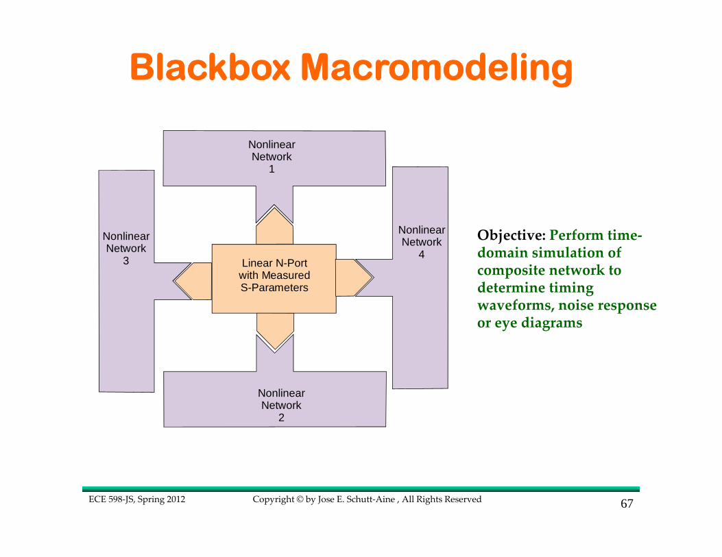
Linear N-Portwith MeasuredS-Parameters
NonlinearNetwork
1
NonlinearNetwork
2
NonlinearNetwork
3
NonlinearNetwork
4Objective: Perform time‐domain simulation of composite network to determine timing waveforms, noise response or eye diagrams
Blackbox Macromodeling

Copyright © by Jose E. Schutt‐Aine , All Rights ReservedECE 598‐JS, Spring 2012 68
Output
Frequency-DomainData
IFFT MOR
DiscreteConvolution
RecursiveConvolution
STAMP
Circuit Simulator
Macromodel Implementation

Copyright © by Jose E. Schutt‐Aine , All Rights ReservedECE 598‐JS, Spring 2012 69
TL Simulation

Copyright © by Jose E. Schutt‐Aine , All Rights ReservedECE 598‐JS, Spring 2012
• Only measurement data is available • Actual circuit model is too complex
Motivations
• Inverse-Transform & Convolution• IFFT from frequency domain data• Convolution in time domain
• Macromodel Approach• Curve fitting• Recursive convolution
Methods
Blackbox Synthesis

Copyright © by Jose E. Schutt‐Aine , All Rights ReservedECE 598‐JS, Spring 2012
Blackbox Synthesis
Terminations are described by a source vector G(ω)and an impedance matrix ZBlackbox is described by its scattering parameter matrix S

Copyright © by Jose E. Schutt‐Aine , All Rights ReservedECE 598‐JS, Spring 2012 72
Blackbox - Method 1
Scattering Parameters ( ) ( ) ( )B S Aω ω ω=
Terminal conditions ( ) ( ) ( )A B TGω ω ω= Γ +
where11 1
o oU ZZ U ZZ−− −⎡ ⎤ ⎡ ⎤Γ = − + −⎣ ⎦ ⎣ ⎦
and11
oT U ZZ−−⎡ ⎤= +⎣ ⎦
(1)
(2)
U is the unit matrix, Z is the termination impedance matrix and Zo is the reference impedance matrix

Copyright © by Jose E. Schutt‐Aine , All Rights ReservedECE 598‐JS, Spring 2012 73
Blackbox - Method 1
Combining (1) and (2) [ ] 1( ) ( ) ( )A U S TGω ω ω−= − Γ
and [ ] 1( ) ( ) ( ) ( ) ( ) ( )B S A S U S TGω ω ω ω ω ω−= = − Γ
[ ][ ] 1( ) ( ) ( ) ( ) ( ) ( )V A B U S U S TGω ω ω ω ω ω−= + = + − Γ
[ ] [ ][ ] 11 1( ) ( ) ( ) ( ) ( ) ( )o oI Z A B Z U S U S TGω ω ω ω ω ω−− −= − = − − Γ
{ }( ) ( )v t IFFT V ω=
{ }( ) ( )i t IFFT I ω=
Copyright © by Jose E. Schutt‐Aine , All Rights ReservedECE 598‐JS, Spring 2012 74
• No Frequency Dependence for TerminationsReactive terminations cannot be simulated
• Only Linear TerminationsTransistors and active nonlinear terminations cannot be described
• StandaloneThis approach cannot be implemented in a simulator
Method 1 - Limitations
Copyright © by Jose E. Schutt‐Aine , All Rights ReservedECE 598‐JS, Spring 2012 75
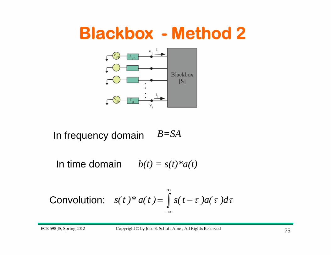
B=SA
b(t) = s(t)*a(t)
s( t )* a( t ) s( t )a( )dτ τ τ∞
−∞
= −∫
In frequency domain
In time domain
Convolution:
Blackbox - Method 2

Copyright © by Jose E. Schutt‐Aine , All Rights ReservedECE 598‐JS, Spring 2012 76
Since a(τ) is known for τ < t, we have:
Isolating a(t)
t 1
1s( t )* a( t ) s( 0 )a( t ) s( t )a( )
τΔτ τ τ Δτ
−
== + −∑
t 1
1H( t ) s( t )a( ) : History
ττ τ Δτ
−
== −∑
t
1s( t )* a ( t ) s( t )a( )
ττ τ Δτ
== −∑
When time is discretized the convolution becomes
Discrete Convolution
Copyright © by Jose E. Schutt‐Aine , All Rights ReservedECE 598‐JS, Spring 2012 77
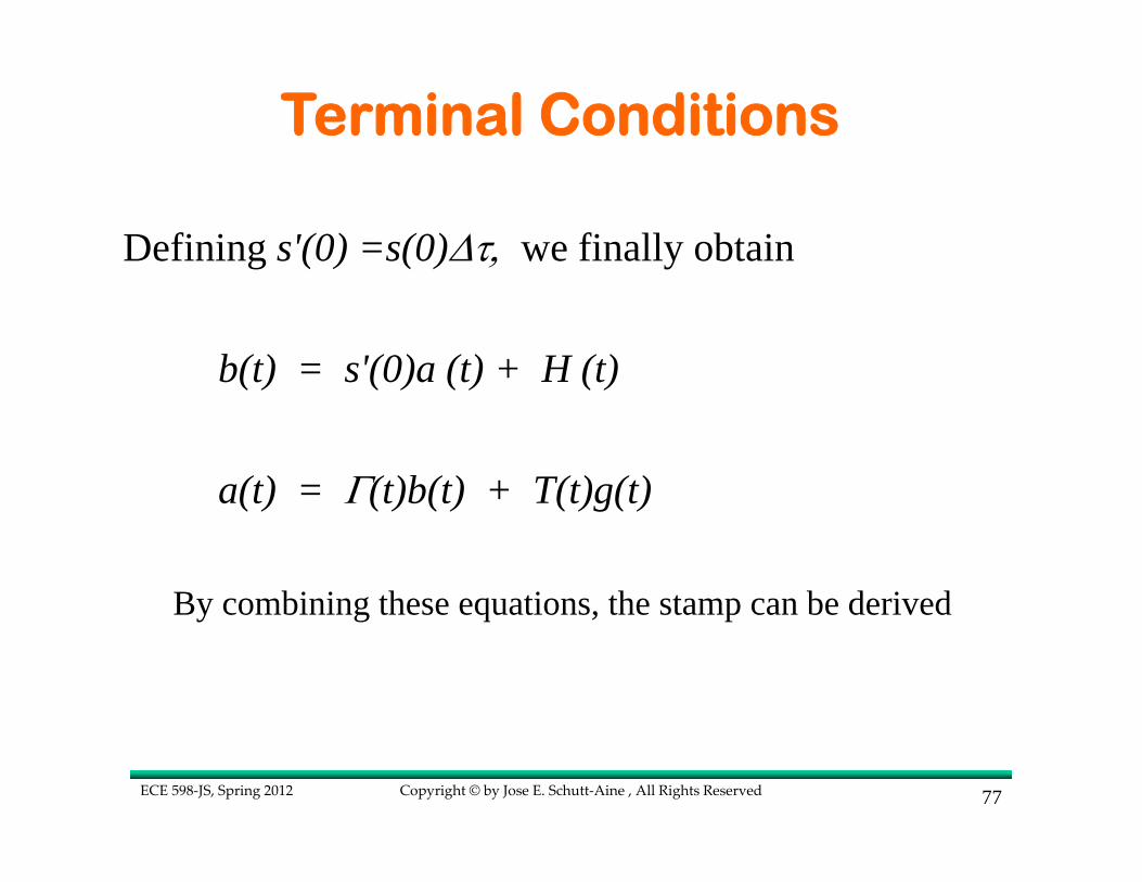
Defining s'(0) =s(0)Δτ, we finally obtain
a(t) = Γ(t)b(t) + T(t)g(t)
b(t) = s'(0)a (t) + H (t)
By combining these equations, the stamp can be derived
Terminal Conditions

Copyright © by Jose E. Schutt‐Aine , All Rights ReservedECE 598‐JS, Spring 2012 78
[ ] [ ]1a(t) 1 (t)s'(0) T(t)g(t) (t)H(t)Γ Γ−= − +
b(t) = s'(0)a (t) + H (t)
[ ]o1a( t ) v( t ) Z i( t )2
= +
[ ]o1b( t ) v( t ) Z i( t )2
= −
The solutions for the incident and reflected wave vectors are given by:
Stamp Equation Derivation
The voltage wave vectors can be related to the voltage and current vectors at the terminals
Copyright © by Jose E. Schutt‐Aine , All Rights ReservedECE 598‐JS, Spring 2012 79
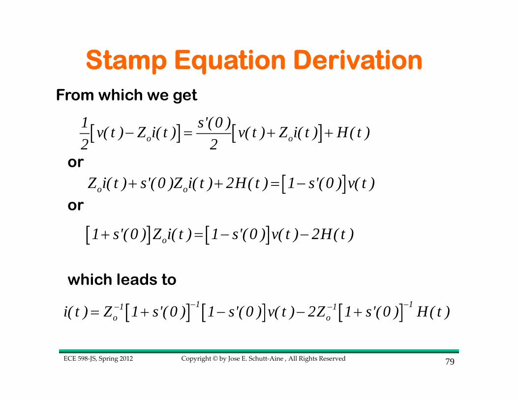
[ ] [ ]o o1 s'( 0 )v( t ) Z i( t ) v( t ) Z i( t ) H( t )2 2
− = + +
[ ]o oZ i( t ) s'(0 )Z i( t ) 2H( t ) 1 s'(0 ) v( t )+ + = −
[ ] [ ]o1 s'(0 ) Z i( t ) 1 s'(0 ) v( t ) 2H( t )+ = − −
[ ] [ ] [ ]1 11 1o oi( t ) Z 1 s'( 0 ) 1 s'( 0 ) v( t ) 2Z 1 s'( 0 ) H( t )− −− −= + − − +
From which we get
Stamp Equation Derivation
or
or
which leads to

Copyright © by Jose E. Schutt‐Aine , All Rights ReservedECE 598‐JS, Spring 2012 80
[ ] [ ]11stamp oY Z 1 s'( 0 ) 1 s'( 0 )−−= + −
[ ] 11stamp oI 2Z 1 s'( 0 ) H( t )−−= +
stamp stampi( t ) Y v( t ) I= −
i(t) can be written to take the form
Stamp Equation Derivation
in which
and

Copyright © by Jose E. Schutt‐Aine , All Rights ReservedECE 598‐JS, Spring 2012 81
[ ] [ ]11stamp oY Z 1 s'( 0 ) 1 s'( 0 )−−= + −
[ ] 11stamp oI 2Z 1 s'(0 ) H( t )−−= +
( ) ( )g stamp g stampY Y v t I I+ = +
stamp stampi( t ) Y v( t ) I= −Stamp Equations

Copyright © by Jose E. Schutt‐Aine , All Rights ReservedECE 598‐JS, Spring 2012 82
No DC Data Point With DC Data Point
If low‐frequency data points are not available, extrapolation must be performed down to DC.
Effects of DC Data

Copyright © by Jose E. Schutt‐Aine , All Rights ReservedECE 598‐JS, Spring 2012 83
-0.2
0
0.2
0.4
0.6
0.8
1
0 2 4 6 8 10
Port 1
Port 1 - No DC ExtrapolationPort 1 - With DC Extrapolation
volts
Time (ns)-0.5
0
0.5
1
1.5
0 2 4 6 8 10 12 14 16
Port 2
Port 2 - No DC ExtrapolationPort 2 - With DC Extrapolation
Vol
ts
Time (ns)
Effect of Low-Frequency Data

Copyright © by Jose E. Schutt‐Aine , All Rights ReservedECE 598‐JS, Spring 2012 84
-2
-1.5
-1
-0.5
0
0 20 40 60 80 100 120
No DC component(lowest freq: 10 MHz)
Vol
ts
Time (ns)
-0.2
0
0.2
0.4
0.6
0.8
1
1.2
0 20 40 60 80 100 120
With DC component
Volts
Time (ns)
Left: IFFT of a sinc pulse sampled from 10 MHz to 10 GHz. Right: IFFT of the same sinc pulse with frequency data ranging from 0-10 GHz. In both cases 1000 points are used
( )2sin 2( )
2ft
V fftπ
π=Calculating inverse Fourier Transform of:
Effect of Low-Frequency Data
Copyright © by Jose E. Schutt‐Aine , All Rights ReservedECE 598‐JS, Spring 2012 85
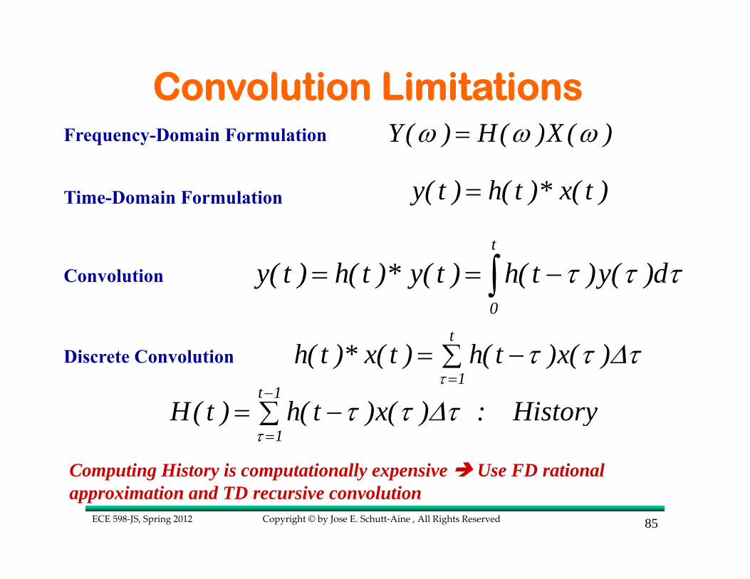
=ω ω ωY( ) H( )X ( )
=y( t ) h( t )* x( t )
Frequency-Domain Formulation
= = −∫ τ τ τt
0
y( t ) h( t )* y( t ) h( t )y( )d
== −∑
ττ τ Δτ
t
1h( t )* x( t ) h( t )x( )
−
== −∑
ττ τ Δτ
t 1
1H( t ) h( t )x( ) : History
Time-Domain Formulation
Convolution
Discrete Convolution
Computing History is computationally expensive Use FD rational approximation and TD recursive convolution
Convolution Limitations

Copyright © by Jose E. Schutt‐Aine , All Rights ReservedECE 598‐JS, Spring 2012 86
Large Network (>1,000 nodes)
Reduced Order Model
(< 30 poles)
SPICE Y(t) v(t) = i(t) Y(ω) V(ω) = I(ω)
Order Reduction
Y(ω) = Y(ω)~ ~
Recursive Convolution
Y(t) v(t) = i(t) ~
11
1 1
( )1 /
Li
i c i
aY Aj
ωω ω=
⎡ ⎤= +⎢ ⎥+⎣ ⎦
∑
Model Order Reduction

Copyright © by Jose E. Schutt‐Aine , All Rights ReservedECE 598‐JS, Spring 2012 87
• AWE – Pade• Pade via Lanczos (Krylov methods)• Rational Function• Chebyshev-Rational function• Vector Fitting Method
11
1 1
( )1 /
Li
i c i
aH Aj
ωω ω=
⎡ ⎤= +⎢ ⎥+⎣ ⎦
∑
Objective: Approximate frequency-domain transfer function to take the form:
Methods
Model Order Reduction

Copyright © by Jose E. Schutt‐Aine , All Rights ReservedECE 598‐JS, Spring 2012 88
Model Order Reduction (MOR)
Question: Why use a rational function approximation?
Lk
k 1 ck
cY( ) H( )X ( ) d X ( )1 j /=
⎡ ⎤= = +⎢ ⎥+⎣ ⎦
∑ω ω ω ωω ω
1
( ) ( ) ( )=
= − + ∑L
pkk
y t dx t T y t
( )( ) ( ) 1 ( )− −= − − + −ω ωck ckT Tpk k pky t a x t T e e y t T
Answer: because the frequency‐domain relation
will lead to a time‐domain recursive convolution:
which is very fast!
where

Copyright © by Jose E. Schutt‐Aine , All Rights ReservedECE 598‐JS, Spring 2012 89
=
= ++∑ω
ω ω
Lk
k 1 ck
cH( ) d1 j /
Transfer function is approximated as
In order to convert data into rational function form, we need a curve fitting scheme Use Vector Fitting
Model Order Reduction

Copyright © by Jose E. Schutt‐Aine , All Rights ReservedECE 598‐JS, Spring 2012
• 1998 - Original VF formulated by Bjorn Gustavsen and Adam Semlyen*
• 2003 - Time-domain VF (TDVF) by S. Grivet-Talocia.
• 2005 - Orthonormal VF (OVF) by Dirk Deschrijver, Tom Dhaene, et al.
• 2006 - Relaxed VF by Bjorn Gustavsen.
• 2006 - VF re-formulated as Sanathanan-Koerner (SK) iteration by W. Hendrickx, Dirk Deschrijver and Tom Dhaene, et al.
History of Vector Fitting (VF)
* B. Gustavsen and A. Semlyen, “Rational approximation of frequency responses by vector fitting,” IEEE Trans. Power Del., vol. 14, no. 3, pp 1052–1061, Jul. 1999

Copyright © by Jose E. Schutt‐Aine , All Rights ReservedECE 598‐JS, Spring 2012 91
Measurement Data
Approximation function
Frequency
S-pa
ram
ete r
FrequencyS-
para
met
e r
Approximation function
Measurement Data S-pa
ram
e ter
Frequency
Measurement Data
Approximation function
Low order Medium order Higher order
LT
CT
LT
CT
LT LT
CT
Orders of Approximation

Copyright © by Jose E. Schutt‐Aine , All Rights ReservedECE 598‐JS, Spring 2012
∗ ∗
∗
=
+ ≥ >*
( ) ( ),[ ( ) ( )] , [ ]0 0T T
H s H sz H s H s z s
− ≥ >*( ) ( ) , [ ]0 0TI H s H s s ,for S-parameters.
,for Y or Z-parameters.
= + ⇔ = +[ ] [ ] [ ] ( ) ( ) ( )ω ω ωe o R Ih n h n h n H j H j jH j
•Accurate:- over wide frequency range.
•Stable:- All poles must be in the left-hand side in s-plane or inside in the unit-circle in z-plane.
•Causal:- Hilbert transform needs to be satisfied.
•Passive:- H(s) is analytic
MOR Attributes

Copyright © by Jose E. Schutt‐Aine , All Rights ReservedECE 598‐JS, Spring 2012 93
• Bandwidth Low-frequency data must be added
• PassivityPassivity enforcement
• High Order of ApproximationOrders > 800 for some serial linksDelay need to be extracted
MOR Problems

Copyright © by Jose E. Schutt‐Aine , All Rights ReservedECE 598‐JS, Spring 2012 94
Length = 7 inches
1.- DISC: Transmission line with discontinuities
2.- COUP: Coupled transmission line2
dx = 51/2 inches
Frequency sweep: 300 KHz – 6 GHz
dxx y
u
z
v
w
Line A
Line B
Examples

Copyright © by Jose E. Schutt‐Aine , All Rights ReservedECE 598‐JS, Spring 2012 95
DISC: Approximation order 90
DISC: Approximation Results

Copyright © by Jose E. Schutt‐Aine , All Rights ReservedECE 598‐JS, Spring 2012 96
-0.2
0
0.2
0.4
0.6
0.8
1
1.2
30 32 34 36 38 40
Exact
B
A
-0.2
0
0.2
0.4
0.6
0.8
1
1.2
30 32 34 36 38 40
Exact
B
A
1 2Microstrip line with discontinuitiesData from 300 KHz to 6 GHz
Observation: Good agreement
DISC: Simulations

Copyright © by Jose E. Schutt‐Aine , All Rights ReservedECE 598‐JS, Spring 2012 97
COUP: Approximation order 75 – Before Passivity Enforcement
COUP: Approximation Results

Copyright © by Jose E. Schutt‐Aine , All Rights ReservedECE 598‐JS, Spring 2012 98
-0.2
-0.1
0
0.1
0.2
0.3
0.4
0.5
0.6
30 35 40 45 50
Exact
B
A
-0.2
-0.1
0
0.1
0.2
0.3
0.4
0.5
0.6
30 35 40 45 50
Convolution
B
A
Port 1: a – Port 2: dData from 300 KHz to 6 GHz
dxx y
a
b
c
d
Observation: Good agreement
COUP: Simulations


![ECE 598 JS Lecture 04 Transmission Linesjsa.ece.illinois.edu/ece598js/Lect_04.pdfTitle Microsoft PowerPoint - Lect_04 [Compatibility Mode] Author jose Created Date 1/19/2012 12:24:22](https://img.dokumen.tips/doc/110x75/5fad2c67beacef572d20dd41/ece-598-js-lecture-04-transmission-title-microsoft-powerpoint-lect04-compatibility.jpg)


![ECE 598 JS Lecture 06 Multiconductorsjsa.ece.illinois.edu/ece598js/Lect_06.pdf · 2013-03-23 · Title: Microsoft PowerPoint - Lect_06 [Compatibility Mode] Author: jose Created Date:](https://img.dokumen.tips/doc/110x75/5e89ff4b3514a836a87544bf/ece-598-js-lecture-06-2013-03-23-title-microsoft-powerpoint-lect06-compatibility.jpg)
![ECE 598 JS Introductionjsa.ece.illinois.edu/ece598js/Lect_01.pdf · Title: Microsoft PowerPoint - Lect_01 [Compatibility Mode] Author: jose Created Date: 1/17/2012 1:29:15 PM](https://img.dokumen.tips/doc/110x75/5f84e80cca6cba696d0d80af/ece-598-js-title-microsoft-powerpoint-lect01-compatibility-mode-author-jose.jpg)