ECE 4524 Artificial Intelligence and EngineeringApplications

Lecture 22: Introduction to LearningReading: AIAMA 18.1-18.3

Today’s Schedule:

I Motivation for Learning

I Types of Learning

I Supervised Learning and Hypothesis spaces

I Example: Decision Trees

Why learning?

I not all information is known at design time

I it might be impractical to program all possibilities directly

I some agents need to be able to adapt over time

I we might not know how to solve a problem directly by design

This area in general is referred to as Machine Learning.

Learning is a very general concept.

It can be applied to all elements of an agents design, e.g. we might

I learn functions mapping percepts to internal states

I learn functions mapping states to actions

I learn the agent model itself

I learn probabilities

I learn utilities of internal states or actions

Any agent component with a representation, prior knowledge ofthe representation, and a way to update the representation usingfeedback can use learning methods.

Categorization of Learning

The most basic distinction in learning is the difference between

I Deductive Learning

I Inductive Learning

Within inductive learning there is

I unsupervised learning

I reinforcement learning

I supervised learning

Supervised Learning

Supervised learning is conceptually very simple, but has manypractical and subtle issues.

I Given a training set consisting of examplesD = {(x1, y1), (x2, y2), · · · , (xn, yn)} where each exampleobeys

yi = f (xi )

for some unknown function f (·).I Find a function, the hypothesis h(·)

y = h(x)

that approximates the true f .

The quality of the approximation is measured using theTest Set.

T = {(x1, y1), (x2, y2), · · · , (xm, ym)}

where m < n and T ∩ D = ∅I Collecting training and testing sets is often hard and expensive

I a h that performs well on the test set is said to generalize well.

I an h that performs well on the training set (said to beconsistent) but poorly on the test set is said to beover-trained.

Note the test set is independent of the training set!

Some Nomenclature

I When y is finite with a categorical interpretation, this is aclassification problem

I If y is binary it is a binary classification problem

I If y is continuous then it is a regression problem.

Hypothesis Space

In y = h(x), h is a hypothesis in some space of functions H.

I Goal is to find a consistent h with smallest testing error andthe simplest representation (Ockham’s Razor)

I If we restrict the space H then it may be that no h can befound which approximates f sufficiently (unrealizable).

I The complexity/expressiveness of H and the generalization ofh ∈ H is related through the bias-variance dilemma.

Bayesian analysis gives us a useful framework forsupervised learning

I Let h ∈ H be parameterized by θ, and the training data givenby D, then the posterior of the parameters is

p(θ|D, h) =p(D|θ, h)p(θ|h)

P(D|h)

I The posterior of the model is the evidence for h

p(h|D) =p(D|h)p(h)

P(D)

where the denominator integrates over all models in H

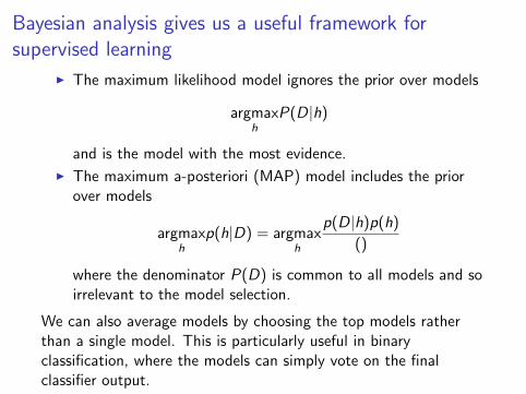
Bayesian analysis gives us a useful framework forsupervised learning

I The maximum likelihood model ignores the prior over models

argmaxh

P(D|h)

and is the model with the most evidence.

I The maximum a-posteriori (MAP) model includes the priorover models

argmaxh

p(h|D) = argmaxh

p(D|h)p(h)()

where the denominator P(D) is common to all models and soirrelevant to the model selection.

We can also average models by choosing the top models ratherthan a single model. This is particularly useful in binaryclassification, where the models can simply vote on the finalclassifier output.

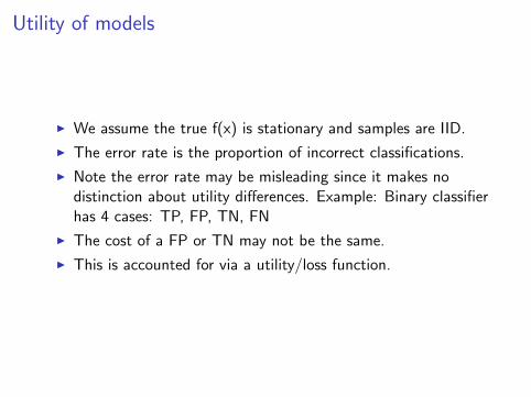
Utility of models

I We assume the true f(x) is stationary and samples are IID.

I The error rate is the proportion of incorrect classifications.

I Note the error rate may be misleading since it makes nodistinction about utility differences. Example: Binary classifierhas 4 cases: TP, FP, TN, FN

I The cost of a FP or TN may not be the same.

I This is accounted for via a utility/loss function.

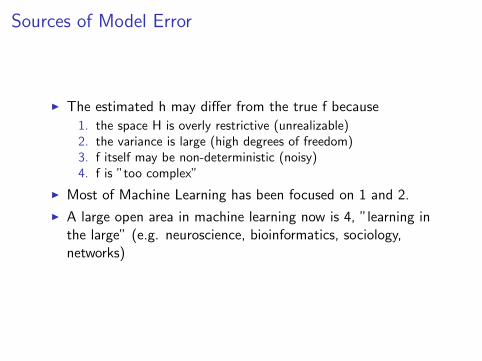
Sources of Model Error

I The estimated h may differ from the true f because

1. the space H is overly restrictive (unrealizable)2. the variance is large (high degrees of freedom)3. f itself may be non-deterministic (noisy)4. f is ”too complex”

I Most of Machine Learning has been focused on 1 and 2.

I A large open area in machine learning now is 4, ”learning inthe large” (e.g. neuroscience, bioinformatics, sociology,networks)

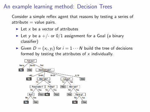
An example learning method: Decision Trees

Consider a simple reflex agent that reasons by testing a series ofattribute = value pairs.

I Let x be a vector of attributes

I Let y be a +/- or 0/1 assignment for a Goal (a binaryclassifier)

I Given D = (xi , yi ) for i = 1 · · ·N build the tree of decisionsformed by testing the attributes of x individually.

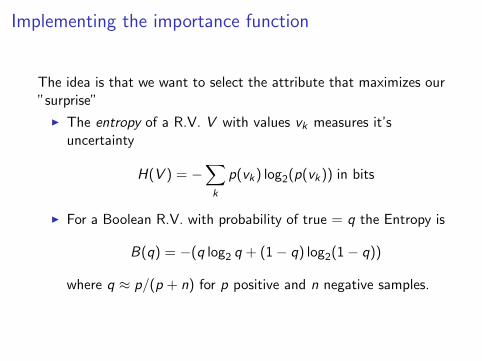
Implementing the importance function

The idea is that we want to select the attribute that maximizes our”surprise”

I The entropy of a R.V. V with values vk measures it’suncertainty

H(V ) = −∑k

p(vk) log2(p(vk)) in bits

I For a Boolean R.V. with probability of true = q the Entropy is

B(q) = −(q log2 q + (1− q) log2(1− q))

where q ≈ p/(p + n) for p positive and n negative samples.

Implementing the importance function

Now suppose we choose attribute A from x

I For each possible value of A we divide the training set into ksubsets with pk positive and nk negative examples

I After testing A, the remaining entropy is

remainder(A) =d∑

k=1

pk + nkp + n

B

(pk

pk + nk

)I The information gain associated with selecting A is then

gain(A) = B

(p

p + n

)− remainder(A)

We choose the attribute with the highest gain in information.

Next Actions

I Reading on Learning Theory (AIAMA 18.4-18.5)

I No warmup.

Reminders:

I Quiz 3 will be Thurday 4/12.

I PS 3 is due tonight.