EC791- International Trade Empirics of Firm-Level ...people.bu.edu/garettos/teaching_docs/firm_productivity.pdf · EC791- International Trade Empirics of Firm-Level Productivity:

1 / 26

EC791- International TradeEmpirics of Firm-Level Productivity: a Survey

Stefania Garetto

Introduction

Introduction

BJRS 2007

BJ 1999

BJ 2004

BJS 2006

Pavcnik 2002

Tybout HIT

RT 1997

2 / 26

When introducing models with heterogeneous firms , we motivated themwith a series of facts highlighting differences in firm-level performancebetween exporters and non-exporters.

Here is a survey of empirical articles on the relationship betweenfirm-level productivity, other measures of performance, and export status.

References:

• Bernard, Jensen, Redding and Schott (2007) JEP, “Firms in International Trade”

• Bernard and Jensen (1999) JIE, “Exceptional Exporter Performance: Cause, Effect, orBoth?”

• Bernard and Jensen (2004) REStat, “Why Some Firms Export”

• Bernard, Jensen and Schott (2006) JME, “Trade Costs, Firms, and Productivity”

• Pavcnik (2002) ReStud, “Trade Liberalization, Exit, and Productivity Improvements”

• Tybout (2005) HIT, “Plant- and Firm-Level Evidence on the ‘New’ Trade Theories”

• Roberts and Tybout (1997) AER, “The Decision to Export in Colombia: An EmpiricalModel of Entry with Sunk Costs”

Bernard, Jensen, Redding and Schott (2007)

Introduction

BJRS 2007

• Limited Participation

• Selection

• Reallocations

• Data

• Other Facts

BJ 1999

BJ 2004

BJS 2006

Pavcnik 2002

Tybout HIT

RT 1997

3 / 26

• JEP article: put the literature into perspective, linking empiricalevidence with the “new trade theory”.

• Establish and describe three main facts:

1. LIMITED PARTICIPATION: not all firms export.

2. SELECTION: exporters are “better” than non-exporters alonga number of dimensions.

3. Effects of trade on REALLOCATIONS AND PRODUCTIVITY(a la Melitz).

Limited Participation

Introduction

BJRS 2007


• Selection

• Reallocations

• Data

• Other Facts

BJ 1999

BJ 2004

BJS 2006

Pavcnik 2002

Tybout HIT

RT 1997

4 / 26

• Among all firms in the U.S. in 2000:

only 4% export;

the top 10% exporters account for 96 % of total exports.

• Among manufacturing firms:

only 18% export;

large variation in participation within manufacturing: only 5% offirms export in “printing and related support”, 38% of firmsexport in “computer and electronic products” ;

exports are a small share of firms’ total sales: from 7% of totalsales in “beverages and tobacco” to 21% in “computer andelectronic products”. The average across sectors is 14%.

Limited Participation

Introduction

BJRS 2007


• Selection

• Reallocations

• Data

• Other Facts

BJ 1999

BJ 2004

BJS 2006

Pavcnik 2002

Tybout HIT

RT 1997

4 / 26

• Among all firms in the U.S. in 2000:

only 4% export;

the top 10% exporters account for 96 % of total exports.

• Among manufacturing firms:

only 18% export;

large variation in participation within manufacturing: only 5% offirms export in “printing and related support”, 38% of firmsexport in “computer and electronic products” ;

exports are a small share of firms’ total sales: from 7% of totalsales in “beverages and tobacco” to 21% in “computer andelectronic products”. The average across sectors is 14%.

⇒ Higher export intensity in more “skill-intensive” sectors? Could be in linewith H-O models... But H-O cannot explain limited participation orintra-industry trade. These aspects call for variety-motivated trade .

Selection

Introduction

BJRS 2007


• Selection

• Reallocations

• Data

• Other Facts

BJ 1999

BJ 2004

BJS 2006

Pavcnik 2002

Tybout HIT

RT 1997

5 / 26

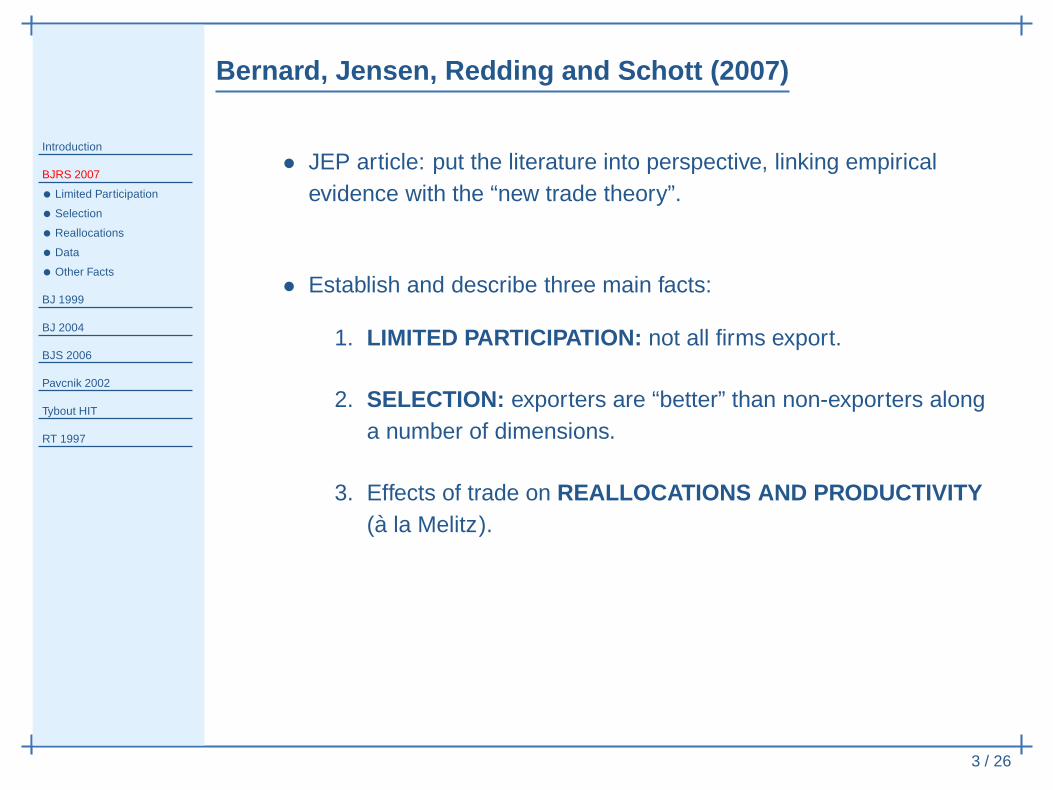
Exporters are different:

1. employ more workers (119% more);

2. have higher sales (148% higher);

3. have higher value-added per worker (26% higher);

4. have higher TFP (2% higher);

5. pay higher wages (17% higher);

6. are more capital-intensive (K/L 32% higher);

7. are more skill-intensive (employ 19% more skilled vs unskilled labor).

Evidence for selection : exporters were different prior to start exporting.Very limited evidence in favor of “learning by exporting”, see BJ (1999).⇓This suggest the existence of entry costs : see Roberts and Tybout (1997),Das, Roberts and Tybout (2007).[Differences in factor intensity do NOT support H-O: we observe the same differences

between exporters and non-exporters across countries.]

Reallocations and Productivity

Introduction

BJRS 2007


• Selection

• Reallocations

• Data

• Other Facts

BJ 1999

BJ 2004

BJS 2006

Pavcnik 2002

Tybout HIT

RT 1997

6 / 26

Trade liberalization induces:

• exit of domestic low-productivity firms

• entry of foreign high-productivity firms

⇓As a result, aggregate productivity increases .

Empirical evidence in support of this mechanism in Pavcnik (2002), lookingat Chilean data, BJS (2006) for the U.S.

Tybout (2005) is a survey of other studies on the topic.

[All this evidence is consistent with the mechanism in Melitz-type models.]

Data

Introduction

BJRS 2007


• Selection

• Reallocations

• Data

• Other Facts

BJ 1999

BJ 2004

BJS 2006

Pavcnik 2002

Tybout HIT

RT 1997

7 / 26

BJRS assembled one of the best existing datasets to study U.S. trade:LFTTD (Linked-Longitudinal Firm Trade Transaction Databa se)

• merges data from U.S. Census and U.S. Customs

• contains all U.S.-related international trade transactions , 1992-2000

• for each transaction, it records:

product

value and quantity

date

trading partner country

transport mode

identity of US firm involved

• ideal to distinguish between firms’ extensive margins (number ofproducts sold/bought, number of export destinations) and intensivemargin (quantity/value traded).

Other Facts

Introduction

BJRS 2007


• Selection

• Reallocations

• Data

• Other Facts

BJ 1999

BJ 2004

BJS 2006

Pavcnik 2002

Tybout HIT

RT 1997

8 / 26

The detail of LFTTD allowed to uncover more detailed statistics:

• Concentration of trade: the top 1% of trading firms by value account for 80% of the

total value of trade

the top 10% of trading firms by value account for 95% of thetotal value of trade

(need a productivity distribution with huge dispersion and/or veryhigh elasticity of substitution to account for this).

• Small trade flows: firms trade small fractions of their total sales

most firms trade with a small number (often 1) of countries(see EKK):

• 64% of U.S. exporters export to 1 destination, and theirtotal export account for 3.3% of total U.S. exports;

• 13.7% of U.S. exporters export to 5 or more destinations,and their total export account for 92.9% of total U.S.exports.

Other Facts (contd.)

Introduction

BJRS 2007


• Selection

• Reallocations

• Data

• Other Facts

BJ 1999

BJ 2004

BJS 2006

Pavcnik 2002

Tybout HIT

RT 1997

9 / 26

• Multiproduct firms:

42.2% of U.S. exporters sell only 1 product abroad, and theyaccount for 0.4% of U.S. total exports

25.9% of U.S. exporters sell 5 products or more abroad, andthey account for 98% of U.S. total exports

positive correlation between the number of products a firmsells and the number of countries it sells to. Both arecorrelated with other firm characteristics.

New papers on multiproduct firms: BRS (2010), Melitz and Ottaviano(2012), Arkolakis and Muendler (2010).

• Importers:

many of the characteristics found for exporters also hold whenlooking at importing firms

many exporters are also importers (see literature on thefragmentation of production).

Bernard and Jensen (1999)

Introduction

BJRS 2007

BJ 1999

• Success and Export

BJ 2004

BJS 2006

Pavcnik 2002

Tybout HIT

RT 1997

10 / 26

On the direction of causality between productivity advantage and exportstatus : are ex-ante good firms that become exporters, or they becomebetter by exporting?

The evidence points towards selection , but to establish it we need to lookat differences in performance before-during-after periods o f export .

Important question, also for export-promotion policy.

Empirical work with US manufacturing data 1984-1992.

Success and Export Status

Introduction

BJRS 2007

BJ 1999


BJ 2004

BJS 2006

Pavcnik 2002

Tybout HIT

RT 1997

11 / 26

3 possibilities:

1. SUCCESS LEADS TO EXPORT: exporting is costly, so only largerand more productive firms can afford it. Hence larger and moreproductive firms become exporters. (SELECTION, modeled inMelitz-type frameworks).

2. EXPORT LEADS TO SUCCESS: exporting is “good for a firm”.Since competition is tougher in foreign markets, firms must “improvetheir performance” to survive there.⇓If true, post-entry performance should be better than pre-entryperformance for exporters.

3. EXPORT ENCOURAGES IMPROVEMENT THAT LEADS TOSUCCESS: firms know that exporting is “good for a firm”, so theydecide to export. Before starting though, they have to undertakeperformance improvements to succeed abroad.

[Notice: 2. and 3. are NOT consistent with optimal behavior!]

Success and Export Status (contd.)

Introduction

BJRS 2007

BJ 1999


BJ 2004

BJS 2006

Pavcnik 2002

Tybout HIT

RT 1997

12 / 26

To distinguish among the 3 possibilities above:

• Look at measures of performance before entry :

divide sample period in 2 sub-periods, and compare:

1. non exporters

2. firms that do not export in the 1st sub-period, but do in the2nd.

⇒ they find that firms that become exporters in the 2nd sub-periodare ex-ante larger, more productive, and pay higher wages thatall-time non-exporters (supports hypothesis 1., but does not exclude2., 3.).


Introduction

BJRS 2007

BJ 1999


BJ 2004

BJS 2006

Pavcnik 2002

Tybout HIT

RT 1997

12 / 26

To distinguish among the 3 possibilities above:

• Look at measures of performance before entry :

divide sample period in 2 sub-periods, and compare:

1. non exporters

2. firms that do not export in the 1st sub-period, but do in the2nd.

⇒ they find that firms that become exporters in the 2nd sub-periodare ex-ante larger, more productive, and pay higher wages thatall-time non-exporters (supports hypothesis 1., but does not exclude2., 3.).

• Look at growth in measures of performance in the yearsimmediately before entry into export

⇒ they find that growth is higher for firms that will start exporting(could support both 2.,3.).


Introduction

BJRS 2007

BJ 1999


BJ 2004

BJS 2006

Pavcnik 2002

Tybout HIT

RT 1997

13 / 26

• Is there an effect of exporting on firm performance? (hyp. 2.)To find out, run reduced-form regressions of changes inperformance measures on initial export status , controlling forother plants characteristics.

Findings:

exporters display higher growth in employment and sales overa 1-year period;

no significant results for other measures of performance andover longer periods.

⇒ Mixed evidence, gives no support to hypothesis 2.NO CONVINCING EVIDENCE THAT EXPORTING LEADS TOPRODUCTIVITY GROWTH!


Introduction

BJRS 2007

BJ 1999


BJ 2004

BJS 2006

Pavcnik 2002

Tybout HIT

RT 1997

13 / 26

• Is there an effect of exporting on firm performance? (hyp. 2.)To find out, run reduced-form regressions of changes inperformance measures on initial export status , controlling forother plants characteristics.

Findings:

exporters display higher growth in employment and sales overa 1-year period;

no significant results for other measures of performance andover longer periods.

⇒ Mixed evidence, gives no support to hypothesis 2.NO CONVINCING EVIDENCE THAT EXPORTING LEADS TOPRODUCTIVITY GROWTH!

• Switching pattern: the data display a lot of entry in/exit from theexport market, suggesting that initial export status is poorlycorrelated with subsequent exporting .⇒ Not much support for the hypothesis that exports lead toimproved performance (hyp. 3.).


Introduction

BJRS 2007

BJ 1999

BJ 2004

BJS 2006

Pavcnik 2002

Tybout HIT

RT 1997

14 / 26

Identify the factors that induce a firm to start exporting . They examine:

1. size

2. labor force composition (quality of workforce)

3. product mix (introduction of new products)

4. past performance

5. entry costs

6. spillovers

7. Government intervention

Census data 1984-1992. Export boom in late 80s generates around 10% ofswitches into and out of exports every year.Probit empirical model to evaluate the effects of the factors above on theprobability of exporting.


Introduction

BJRS 2007

BJ 1999

BJ 2004

BJS 2006

Pavcnik 2002

Tybout HIT

RT 1997

14 / 26

Identify the factors that induce a firm to start exporting . They examine:

1. size ⇒ pos. corr. with export

2. labor force composition (quality of workforce) ⇒ pos. corr. with export

3. product mix (introduction of new products) ⇒ pos. corr. with export

4. past performance ⇒ most important factor

5. entry costs ⇒ significant effect (see also RT 1997, DRT 2007)

6. spillovers ⇒ no effect

7. Government intervention ⇒ no effect

Census data 1984-1992. Export boom in late 80s generates around 10% ofswitches into and out of exports every year.Probit empirical model to evaluate the effects of the factors above on theprobability of exporting.

Bernard, Jensen and Schott (2006)

Introduction

BJRS 2007

BJ 1999

BJ 2004

BJS 2006

Pavcnik 2002

Tybout HIT

RT 1997

15 / 26

Attempt to test trade-induced reallocations and their effect on aggregateproductivity (the “Melitz” mechanism).

Link plant-level U.S. manufacturing data with industry measures of tariffsand transportation costs.

As trade costs fall:

1. industry productivity increases

2. higher probability of plant death

3. higher probability of successful exports

4. existing exporters increase their export shipments.

(all the empirical findings are in line with the mechanism of the Melitzmodel).

Pavcnik (2002)

Introduction

BJRS 2007

BJ 1999

BJ 2004

BJS 2006

Pavcnik 2002

• Results

Tybout HIT

RT 1997

16 / 26

Empirical investigation of the effects of trade liberalization onproductivity in the case of Chile.

Outline:

1. Structural estimation of a production function to obtain estimates ofplant-level productivity, controlling for selection, simultaneity bias,and plant exit.

2. Relate changes in productivity to trade liberalization by exploitingvariation over time and across traded and non-traded sectors.

Pavcnik (2002) (contd.)

Introduction

BJRS 2007

BJ 1999

BJ 2004

BJS 2006

Pavcnik 2002

• Results

Tybout HIT

RT 1997

17 / 26

Findings:

• Support for within-plant productivity improvements related totrade liberalization:

the productivity of plants in the traded sectors grew 3-10%more than in the non-traded sectors;

exiting plants are on average 8% less productive than survivingplants.


Introduction

BJRS 2007

BJ 1999

BJ 2004

BJS 2006

Pavcnik 2002

• Results

Tybout HIT

RT 1997

17 / 26

Findings:




• Results seem to contradict the absence of within-firm effects found inBernard and Jensen (1999), but the two papers are testing twodifferent things:

Bernard and Jensen (1999) find no evidence that exportingaffects the productivity of an exporting plant;

Pavcnik (2002) test whether opening to trade increases theproductivity of domestic plants, independently on whether theytrade or not (import competition channel : firms must “trimtheir fat” to survive).


Introduction

BJRS 2007

BJ 1999

BJ 2004

BJS 2006

Pavcnik 2002

• Results

Tybout HIT

RT 1997

17 / 26

Findings:




• Results seem to contradict the absence of within-firm effects found inBernard and Jensen (1999), but the two papers are testing twodifferent things:

Bernard and Jensen (1999) find no evidence that exportingaffects the productivity of an exporting plant;

Pavcnik (2002) test whether opening to trade increases theproductivity of domestic plants, independently on whether theytrade or not (import competition channel : firms must “trimtheir fat” to survive).

• Aggregate productivity improvements are linked to exit: reshuffling ofresources from less efficient to more efficient plants (a la Melitz).

Tybout, Handbook of International Trade

Introduction

BJRS 2007

BJ 1999

BJ 2004

BJS 2006

Pavcnik 2002

Tybout HIT

• Static

• Dynamics

RT 1997

18 / 26

Survey of firm-level and plant-level evidence on the relationships betweenpricing, firm size, export status, productivity and profitab ility .

RESULTS AND “STATIC” EVIDENCE:

1. mark-ups fall with import competition;

2. trade competition has effects on firm-level sales (on average, theydecline);

3. trade rationalizes production : the most efficient plants expand,while the least efficient contract;

4. trade increases aggregate productivity , via both scale effects andreallocations;

5. trade competition can also affect intra-firm efficiency (mixedevidence).

Tybout, Handbook of International Trade (contd.)

Introduction

BJRS 2007

BJ 1999

BJ 2004

BJS 2006

Pavcnik 2002

Tybout HIT

• Static

• Dynamics

RT 1997

19 / 26

EVIDENCE ON TRANSITIONAL DYNAMICS:Interaction between sunk costs, firm heterogeneity, and uncertainty .(More complex issue to address, rely on dynamic stochastic optimization).

• First papers: Dixit (1989), Baldwin and Krugman (1989): role of sunkcosts and expectations in ruling exporters’ behavior.

history-dependence: decisions depend on whether a firm is inor out of the market;

aggregate outcomes depend on the % of firms in each state.

hysteresis.

• Roberts and Tybout (1997), Das, Roberts and Tybout (2007):empirical relevance of the sunk-cost export model.

sunk costs are important, and more so for small firms;

aggregate exports are rel. insensitive to history andexpectations.

MORE RECENT:

• Eaton et al. (2011): learning from exporting as the core mechanismbehind entry and exit of small exporters.

Roberts and Tybout (1997)

Introduction

BJRS 2007

BJ 1999

BJ 2004

BJS 2006

Pavcnik 2002

Tybout HIT

RT 1997

• Notation

• Model

• Estimation

• Results

20 / 26

• Main idea:

non-exporters must pay a sunk cost to enter a foreign market(and become exporters);

if a positive shock induces entry , its reversal may not induceexit ⇒ hysteresis in trade flows.

• Test the existence of sunk costs-induced hysteresis by analyzingentry and exit patterns in the data.

• Dynamic discrete choice model :

current export status is a function of previous exportingexperience , other firm characteristics, and unobserved seriallycorrelated shocks;

the conditional effect of a plant’s exporting history on currentexport status can be used to infer the importance of sunkcosts.

• Data on Colombian manufacturing plants, 4 industries, 1981-1989.

Roberts and Tybout (1997): Notation

Introduction

BJRS 2007

BJ 1999

BJ 2004

BJS 2006

Pavcnik 2002

Tybout HIT

RT 1997

• Notation

• Model

• Estimation

• Results

21 / 26

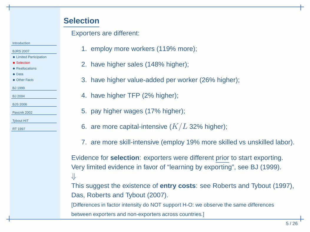
πit(pt, sit): expected profits if exporting - expected profits if notexporting for plant i at time t;

pt: market-level variables (exchange rates, demand levels, ...);sit: plant-specific state variables;

F ji : sunk cost of starting to export for plant i if it last exported

at time t− j (for j ≥ 2);F 0i : sunk cost of starting to export for plant i if it never exported

before;Xi: loss of exiting the export market for plant i

Yit =

1 ; if i exports at time t

0 ; otherwise.

Y(−)it = Yi,t−j |j = 0, ...Ji

where Ji denotes the age of plant i (Y(−)it is the exporting history of plant

i).

Roberts and Tybout (1997): Model

Introduction

BJRS 2007

BJ 1999

BJ 2004

BJS 2006

Pavcnik 2002

Tybout HIT

RT 1997

• Notation

• Model

• Estimation

• Results

22 / 26

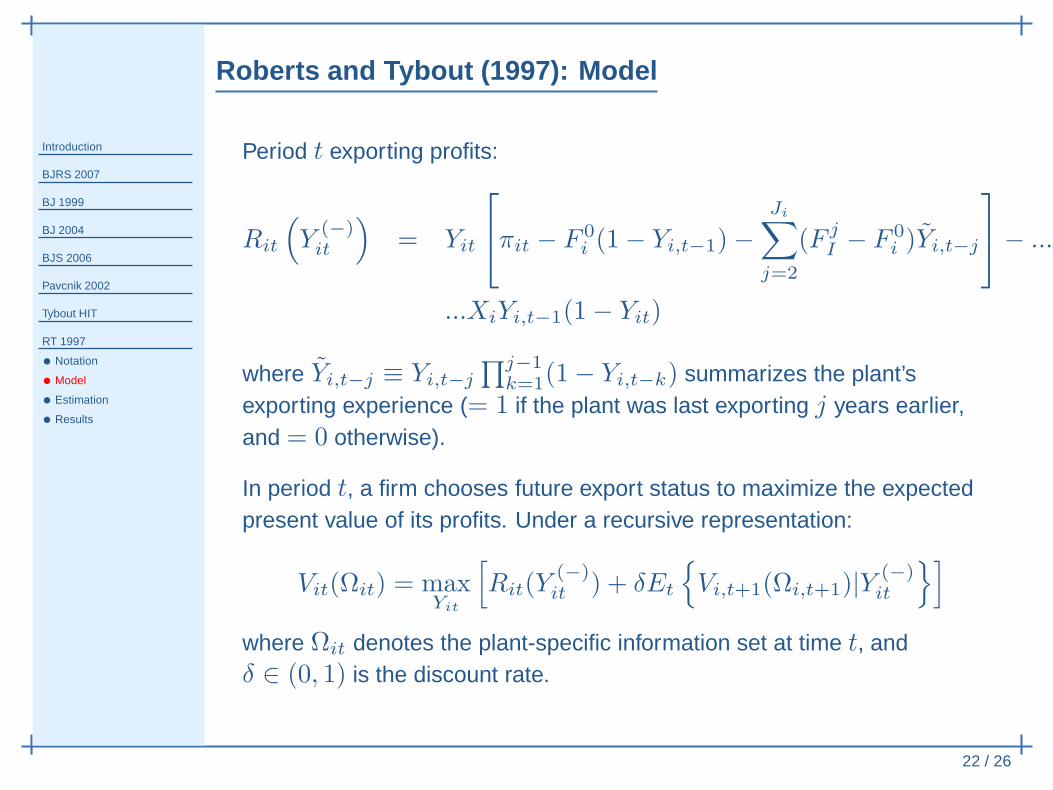
Period t exporting profits:

Rit

(

Y(−)it

)

= Yit

πit − F 0i (1− Yi,t−1)−

Ji∑

j=2

(F jI − F 0

i )Yi,t−j

− ...

...XiYi,t−1(1− Yit)

where Yi,t−j ≡ Yi,t−j

∏j−1k=1(1− Yi,t−k) summarizes the plant’s

exporting experience (= 1 if the plant was last exporting j years earlier,and = 0 otherwise).

In period t, a firm chooses future export status to maximize the expectedpresent value of its profits. Under a recursive representation:

Vit(Ωit) = maxYit

[

Rit(Y(−)it ) + δEt

Vi,t+1(Ωi,t+1)|Y(−)it

]

where Ωit denotes the plant-specific information set at time t, andδ ∈ (0, 1) is the discount rate.

Roberts and Tybout (1997): Model (contd.)

Introduction

BJRS 2007

BJ 1999

BJ 2004

BJS 2006

Pavcnik 2002

Tybout HIT

RT 1997

• Notation

• Model

• Estimation

• Results

23 / 26

Participation condition. Plant i exports at time t if:

πit(pt, sit)︸︷︷︸

profit flow

+ δ [Et(Vi,t+1(Ωi,t+1)|Yit = 1)− Et(Vi,t+1(Ωi,t+1)|Yit = 0)]︸︷︷︸

continuation value

≥ ...

F 0I

︸︷︷︸

cost of first entry

− (F 0I +Xi)Yi,t−i

︸︷︷︸

cost of exit

+

Ji∑

j=2

(F 0I − F

ji )Yi,t−j

︸︷︷︸

cost of entry after j periods without exporting

Let π∗

it denote the left-hand side of the participation condition: π∗

it is alatent variable representing the expected increment to gross future profitsfor plant i if it exports at t.

Dynamic discrete choice equation:

Yit =

1 ; if π∗

it − F 0I + (F 0

I +Xi)Yi,t−i +

Ji∑

j=2

(F 0I − F j

i )Yi,t−j ≥ 0

0 ; otherwise.

Roberts and Tybout (1997): From Model to Estimation

Introduction

BJRS 2007

BJ 1999

BJ 2004

BJS 2006

Pavcnik 2002

Tybout HIT

RT 1997

• Notation

• Model

• Estimation

• Results

24 / 26

Assume: π∗

it − F 0i = µt + βZit + εit.

The term π∗

it − F 0I

summarizes exogenous plant and market characteristics. The authors

assume it is composed by a time effect µt (which captures temporal variation in profitability

and start-up costs common to all plants: credit market conditions, exchange rates, trade

policy), by observable plant-specific determinants of profits and start-up costs Zit (industry

dummies, ownership, location, prices, wages, capital, age), and by an error term εit.

Also assume: F 0i = F 0, F j

i = F j , Xi = X (sunk costs are common across

plants).

Define: γ0 ≡ F 0 +X , γj ≡ F 0 − F j .

Estimating equation:

Yit =

1 ; if µt + βZit + γ0Yi,t−i +

Ji∑

j=2

γj Yi,t−j + εit ≥ 0

0 ; otherwise.

Testing the null hypothesis that sunk costs are NOT important is equivalentto test whether γ0 and γj are jointly equal to 0.

Roberts and Tybout (1997): Estimation

Introduction

BJRS 2007

BJ 1999

BJ 2004

BJS 2006

Pavcnik 2002

Tybout HIT

RT 1997

• Notation

• Model

• Estimation

• Results

25 / 26

Potential issues:

1. Persistence in status may be due to sources other than sunk costs,which are not included into Zit and can induce serial correlation ofεit.

Solution: Roberts and Tybout allow for serial correlation of the error term:

εit = αi + ωit, where ωit = ρωi,t−1 + ηit.

2. In a sample of T periods, the lag structure implies that we can runthe estimation equation only from year J + 1 to year T , but onecannot treat Yi,t−i and Yi,t−j as exogenous variables for the first Jyears (“initial condition problem”) .

Solution: following Heckman (1981), Roberts and Tybout use an “approximate”representation of Yit for t = 1, ...J :

π∗

it − F 0i = λZ

pit+ ε

pit

Yit =

1 ; if λZpit + ε

pit ≥ 0

0 ; otherwise.

where εpit = α

pi + ω

pit, ωp

it = ρpωpi,t−1 + η

pit, and αi and α

pi are correlated.

Roberts and Tybout (1997): Estimation and Results

Introduction

BJRS 2007

BJ 1999

BJ 2004

BJS 2006

Pavcnik 2002

Tybout HIT

RT 1997

• Notation

• Model

• Estimation

• Results

26 / 26

Estimation performed via simulated method of moments :

• choose an initial set of parameter values;

• by combining the distribution of errors and the observable variables,simulate Yit for each plant;

• search over the parameter space to obtain trajectories for Yit thatare as similar as possible to the export dynamics observed in thedata.

Results:

• The Wald test on the estimates of γ0, γj REJECTS the nullhypothesis that the sunk costs are zero:sunk costs are important, exporting history matters!

• Recent history matters the most: previous year exporting status isthe most significant variable in predicting current export status.

• Export status at longer lags is not as important: after a two-yearabsence from the export market, re-entry costs are NOT significantlydifferent from first-time entry costs.

Documents

EC791- International Trade Empirics of Firm-Level ...people.bu.edu/garettos/teaching_docs/firm_productivity.pdf · EC791- International Trade Empirics of Firm-Level Productivity: