Lecture 7: Assignment Models (Empirics) - Dave …dave-donaldson.com/.../10/Lecture-7-Assignment-Models-empirics.pdf · { Lecture 7: Assignment Models (Empirics) ... agriculture As

Econ 266: International Trade– Lecture 7: Assignment Models (Empirics) –

Stanford Econ 266 (Donaldson)

Winter 2016 (lecture 7)

Stanford Econ 266 (Donaldson) Assignment Models (Empirics) Winter 2016 (lecture 7) 1 / 81

Plan of Today’s Lecture

1 Introduction to assignment models

2 Empirical applications of (Ricardian) assignment models:1 Testing Ricardian comparative advantage: Costinot and Donaldson

(2012a)2 Gains from economic integration: Costinot and Donaldson (2012b)3 Climate change and trade: Costinot, Donaldson and Smith (2016)



1 Introduction to assignment model empirics


(2012a)2 Gains from economic integration: Costinot and Donaldson (2012b)3 Climate change and trade: Costinot, Donaldson and Smith (2016)


Introduction

Following from last lecture, we now consider empirical applications ofassignment models (of sort in Costinot-Vogel, 2015 survey)

We will place particular emphasis on settings in which:

Each fundamental production unit uses one factor (land). This is ofcourse what makes these Ricardian assignment models.But the observable production units are comprised of many suchfundamental production units, each of which is unique (i.e. the type ofland is different).Fundamental production units combine as perfect substitutes togenerate output at the observable level.So at the level of the observable production unit, this is an ‘assignmentmodel’ of the comparative advantage and Ricardian sort, as seen inLecture 6.



1 Introduction to Ricardian assignment models

2 Empirical applications of (Ricardian) assignment models:1 Testing Ricardian comparative advantage: Costinot and

Donaldson (2012a)2 Gains from economic integration: Costinot and Donaldson (2012b)3 Climate change and trade: Costinot, Donaldson and Smith (2016)


A Key Empirical Challenge

Suppose that different factors of production specialize in differenteconomic activities based on their relative productivity differences

Following Ricardo’s famous example, if English workers are relativelybetter at producing cloth than wine compared to Portuguese workers:

England will produce clothPortugal will produce wineAt least one of these two countries will be completely specialized in oneof these two sectors

Accordingly—as discussed in Lecture 5—the key explanatory variablein Ricardo’s theory, relative productivity, cannot be directly observed


How Can One Solve This Identification Problem?Existing Approach

Previous identification problem is emphasized by Deardorff (1984) inhis review of empirical work on the Ricardian model of trade

A similar identification problem arises in labor literature in whichself-selection based on CA is often referred to as the Roy model

Heckman and Honore (1990): if general distributions of worker skillsare allowed, the Roy model has no empirical content

One Potential Solution:

Make (fundamentally untestable) functional form assumptions aboutdistributionsUse these assumptions to relate observable to unobservableproductivity,

Examples:

In a labor context: Log-normal distribution of worker skillsIn a trade context: Frechet distributions across countries and industries(Costinot, Donaldson and Komunjer, 2012)


How Can One Solve This Identification Problem?This Paper’s Approach

Focus on sector in which scientific knowledge of how essential inputsmap into outputs is well understood: agriculture

As a consequence of this knowledge, agronomists predict theproductivity of a ‘field’ (small parcel of land) if it were to grow anyone of a set of crops

In this particular context, we know the productivity of a ‘field’ in alleconomic activities, not just those in which it is currently employed


Basic Theoretical Environment

The basic environment is the same as in the purely Ricardian part ofCostinot (2009)

Consider a world economy comprising:

c = 1, ...,C countriesg = 1, ...,G goods [crops in our empirical analysis]f = 1, ...,F factors of production [‘fields’, or grid cells, in our empiricalanalysis]

Factors are immobile across countries, perfectly mobile across sectors

Lcf ≥ 0 denotes the inelastic supply of factor f in country c

Factors of production are perfect substitutes within each country andsector, but vary in their productivities Ag

cf ≥ 0


Cross-Sectional Variation in Output

Total output of good g in country c is given by

Qgc =

F∑f =1

Agcf L

gcf

Take producer prices pgc ≥ 0 as given and focus on the allocation that

maximizes total revenue at these prices

Assuming that this allocation is unique, can express output as

Qgc =

∑f ∈Fg

c

Agcf Lcf (1)

where Fgc is the set of factors allocated to good g in country c :

Fgc = { f = 1, ...F |Ag

cf /Ag ′

cf > pg ′c /p

gc if g ′ 6= g} (2)


Data Requirements

CD (2012a; AER P&P)’s test of Ricardo’s ideas requires data on:

Actual output levels, which we denote by Qgc

Data to compute predicted output levels, which we denote by Qgc

By equations (1) and (2), we can compute Qgc using data on:

Productivity, Agcf , for all factors of production f

Endowments of different factors, Lcf

Producer prices, pgc


Output and Price Data

Output (Qgc ) and price (pg

c ) data are from FAOSTAT

Output is equal to quantity harvested and is reported in tonnes

Producer prices are equal to prices received by farmers net of taxesand subsidies and are reported in local currency units per tonne

In order to minimize the number of unreported observations, our finalsample includes 55 countries and 17 crops

Since Ricardian predictions are cross-sectional, all data are from 1989


Productivity Data

Global Agro-Ecological Zones (GAEZ) project run by FAO

Used in Nunn and Qian (2011) as proxy for areas where potato couldbe grown

Productivity (Agcf ) data for:

154 varieties grouped into 25 crops c (though only 17 are relevant here)All ‘fields’ f (5 arc-minute grid cells) on Earth

Inputs:

Soil conditions (8 dimensional vector)Climatic conditions (rainfall, temperature, humidity, sun exposure)Elevation, average land gradient.

Modeling approach:

Entirely ‘micro-founded’ from primitives of how each crop is grown.64 parameters per crop, each from field and lab experiments.Different scenarios for other human inputs. We use ‘mixed, irrigated’


Example: Relative Wheat-to-Sugar Cane Productivity


Empirical Strategy

To overcome identification problem highlighted by Deardorff (1984)and Heckman and Honore (1990), CD (2012a) follow two-stepapproach:

1 We use the GAEZ data to predict the amount of output (Qgc ) that

country c should produce in crop g according to (1) and (2)2 We regress observed output (Qg

c ) on predicted output (Qgc )

Like in HOV literature, they consider test of Ricardo’s theory ofcomparative advantage to be a success if:

The slope coefficient in this regression is close to unityThe coefficient is precisely estimatedThe regression fit is good

Compared to HOV literature, CD (2012a) estimate regressions in logs:

Core of theory lies in how relative productivity predict relative quantitiesAbsolute levels of output are far off because more uses of land than 17crops


Results





(2012a)2 Gains from economic integration: Costinot and Donaldson

(2012b)3 Climate change and trade: Costinot, Donaldson and Smith (2016)


Recall a Classic Question in this Course: How Large arethe Gains from Economic Integration?

Regions of the world, both across and within countries, appear to havebecome more economically integrated with one another over time.

Two natural questions arise:

1 How large have been the gains from this integration?

2 How large are the gains from further integration?


How Large are the Gains from Economic Integration?

Deardorff (1984) identification problem arises again.

Fundamental challenge lies in predicting how local markets wouldbehave under counterfactual scenarios in which they become moreor less integrated with rest of the world.

In a Trade context, counterfactual scenarios typically involve thereallocation of multiple factors of production towards differenteconomic activities.

Hence researcher requires knowledge of counterfactual productivityof factors if they were employed in sectors in which producers arecurrently, and deliberately, not using them.

Any study of the gains from economic integration needs to overcomethis identification problem.


How to Overcome Identification Problem?

Four main approaches in the literature:

“Reduced form” approach (e.g. Frankel and Romer 1999): knowledgeof CF obtained by observing behavior of “similar but open” countries(Lecture 2).

“Autarky” approach (e.g. Bernhofen and Brown, 2005): autarky prices,when observed, are useful (Lecture 2).

“Sufficient statistic” approach (e.g. Chetty, 2009): knowledge of CFtechnologies unnecessary (for small changes) because gains fromreallocation of production are second-order at optimum.

“Structural” approach (e.g. Eaton and Kortum 2002): knowledge ofCF obtained by extrapolation based on (untestable) functional forms(Lecture 4).

Basic idea of CD (2012b):

Develop new structural approach with weaker need for extrapolation byfunctional form assumptions by drawing on agronomic knowledge inagricultural sector (from CD2012a).


CD (2012b): Method

Consider a panel of ∼1,500 U.S. counties from 1880 to 1997.

Choose US for long sweep of high-quality, comparable micro-data fromimportant agricultural economy.

Use Roy/Ricardian model + FAO data to construct PPF in eachcounty.

Then two steps:1 Measuring Farm-gate Prices:

We combine Census data on output and PPF to infer prices thatfarmers in local market i appear to have been facing.

2 Measuring Gains from Integration:

We compute the spatial distribution of price gaps between U.S.counties and New York/World in each year.

We then ask: “For any period t, how much higher (or lower) would thetotal value of US agricultural output in period t have been if price gapswere those from 1997 rather than those from period t?”


Inferring farm-gate pricesSometimes effects are clearly visible (eg US-Canada 49th parallel border)


CD (2012b): Results

Farm-gate price estimates look sensible:

State-level price estimates correlate well with state-level price data.

How large have been the gains that arose as counties becameincreasingly integrated?

eg 1880-1920: 2.3 % growth (in agricultural GDP) per yearsame order of magnitude as productivity growth in agriculture


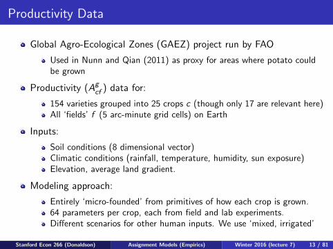
A Few Caveats to Keep in Mind

1 FAO data are only available in 2011.

Extrapoloation necessary when going back in time.

To do so CD (2012b) allow unrestricted county-crop-year specificproductivity shocks.

2 Highest resolution output data available (from Census) is atcounty-level.

So direct predictions from high-resolution FAO model, pixel by pixel,are not testable.

3 Land (though heterogeneous) is the only factor of production.

Should think of land as “equipped” land


Basic Environment

Many ‘local’ markets i ∈ I ≡{1, ..., I} in which production occurs

One ‘wholesale’ market in which goods are sold (New York/World)

Only factors of production are fields f ∈ Fi ≡ {1, ...,Fi}V f

i ≥ 0 denotes the number of acres covered by field f in market i

Fields can be used to produce multiple goods k ∈ K ≡{1, ...,K + 1}

Goods k = 1, ...,K are ‘crops’; Good K + 1 is an ‘outside’ good

Total output Qkit of good k in market i is given by

Qkit =

∑f ∈Fi

Afkit L

kfit

All fields have same productivity in outside sector: AfK+1it = αK+1

it


Basic Environment (Continued)

Large number of price-taking farms in all local markets.

Profits of farm producing good k in local market i are given by:

Πkit = pk

it

∑f ∈Fi

Afkit L

kfit

−∑f ∈Fi

r fitL

fkit ,

where farm-gate price of good k in local market i is given by:

pkit ≡ pk

t /(1 + τkit ).

Profit maximization by farms requires:

pkitA

fkit − r f

it ≤ 0, for all k ∈ K, f ∈ Fi , (3)

pkitA

fkit − r f

it = 0, if Lfkit > 0, (4)

Factor market clearing in market i requires:∑k∈K

Lfkit ≤ V f

i , for all f ∈ Fi . (5)


Competitive Equilibrium

Notation:

pt ≡ (pkt )k∈K is exogenously given vector of wholesale prices

pit ≡(pk

it

)k∈K is the vector of farm gate prices

rit ≡ (r fit)f∈F is the vector of field prices

Lit ≡ (Lfkit )k∈K,f∈F is the allocation of fields to goods in local market i

Definition

A competitive equilibrium in a local market i at date t is a field allocation,Lit , and a price system, (pit , rit), such that conditions (3)-(5) hold.


Two Steps of Analysis

Recall that CD (2012b) break analysis down into two steps:

1 Measuring Farm-gate Prices:

Combine data on output (from the Census) and the PPF (from theFAO) to infer the crop prices (pk

it) that farmers in local market i appearto have been facing.

2 Measuring Gains from Integration:

Compute price gaps (1 + τ kit ) as the difference between farm-gate prices

and prices in wholesale markets.

Then ask how much more productive a collection of local markets iwould be under a particular counterfactual ‘integration’ scenario: allmarkets i face lower price gaps.

Now describe how to do these steps in turn.


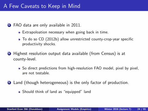
Measuring Farm-gate PricesAssumptions about technological change

The FAO aims for its measures of counterfactual productivity(Afk

i ,2011) to be relevant today (ie in 2011). But how relevant are

these measures for true technology (Afkit ) in, eg, 1880?

With data on both output and land use, by crop, CD (2012b) needonly the following assumption:

Afkit = αk

itAfki ,2011, for all k = 1, ...,K , f ∈ Fi .

How realistic is this assumption?

The FAO runs model under varied conditions (eg irrigation vs rain-fed).

R2 of ln Afki,scenario2 − ln Afk

i,scenario1 on crop-county fixed effects is0.78-0.82.

Results are insensitive to using these alternative scenarios.


Measuring Farm-gate Prices

Dataset contains the following measures, which we assume are relatedto their theoretical analogues in the following manner:

Sit =K∑

k=1

pkitQ

kit ,

Qkit = Qk

it , for all k = 1, ...,K ,

Lkit =

∑f ∈Fi

Lfkit , for all k = 1, ...,K ,

V fi = V f

i , for all f ∈ Fi .

Definition

Given an observation Xit ≡ [Sit , Qkit , L

kit , V

fi , A

fki ,2011], a vector of

productivity shocks and farm gate prices, (αit , pit), is admissible if andonly if there exist a field allocation, Lit , and a vector of field prices, rit ,such that (Lit , pit , rit) is a competitive equilibrium consistent with Xit .


Measuring Farm-gate PricesNotation

For any observation Xit , we denote:

K∗it ≡ {k : Qkit > 0}

A∗it ≡ {α : αk > 0 if k ∈ K∗it}

P∗it ≡ {p : pk > 0 if k ∈ K∗it}

Li ≡{L :∑

k∈K Lfk ≤ V fi

}L (αit ,Xit) ≡ arg maxL∈Li mink∈K∗

it

{∑f∈Fi

αkitA

fki,2011L

fk/Qkit

}


Theorem

For any Xit ∈ X , the set of admissible vectors of productivity shocks andgood prices is non-empty and satisfies: (i) if (αit , pit) ∈ A∗it × P∗it isadmissible, then

(αk

it

)k∈K∗it/{K+1} is equal to unique solution of∑

f ∈Fαk

itAfki2011L

fkit = Qk

it for all k ∈ K∗it/ {K + 1} , (6)∑f ∈Fi

Lfkit = Lk

it for all k ∈ K∗it/ {K + 1} , (7)

with Lit ∈ L (αit ,Xit) and (ii) conditional on αit ∈ A∗it , Lit ∈ L (αit ,Xit)satisfying (6) and (7), (αit , pit) ∈ A∗it × P∗it is admissible iff∑

k∈K∗i /{K+1}

pkitQ

kit = Sit ,

αk ′it p

k ′it A

fk ′i2011 ≤ αk

itpkitA

fki2011 for all k,k ′ ∈ K, f ∈ Fi , if Lfk

it > 0.


Measuring Farm-gate PricesResults

Corollary

For almost all Xit ∈ X ,(pk

it

)k∈K∗it/{K+1} is equal to the unique solution of∑

k∈K∗i /{K+1}

pkitQ

kit = Sit ,

pk ′it

pkit

=αk

itAfki2011

αk ′it A

fk ′i2011

, for any f ∈ Fi s.t. Lfkit × Lfk ′

it > 0,

where(αk

it

)k∈K∗it/{K+1} and Lit are as described in previous theorem.


Measuring Farm-gate PricesIn practice, for a county that can be illustrated in 2-dimensions
















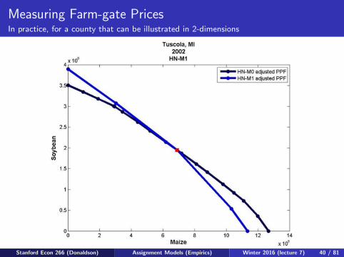
Measuring Farm-gate PricesComputation

Computation of αit and pit is non-trivial in high dimensional settingslike those we consider.

For example, median county has F = 26 and K∗ = 8.

Hence, (K∗)F = 3× 1023 fully specialized allocations to consider justto construct kinks of PPF.

Then ∼1,500 counties times 16 time periods.

Theorem 1 is useful in this regard:

‘Inner loop’: Conditional on αit , farm-gate prices can be inferred bysolving a simple linear programming problem.

‘Outer loop’: αit is relatively low-dimension (K∗).

Paper develops algorithm that speeds up outer loop (standardalgorithms too slow).


Measuring Gains from Economic IntegrationCounterfactual

Recall that CD (2012b)’s counterfactual question is:

“For any pair of periods, t and t ′, how much higher (or lower)would the total value of agricultural output in period t have beenif price gaps were those of period t ′ rather than period t?”

Let(Qk

it

)′denote counterfactual output level if farmers in market i

were facing(pk

it

)′= pk

t /(1 + τkit′) rather than pk

it = pkt /(1 + τk

it ).

Then measure the gains (or losses) from changes in the degree ofeconomic integration as:

∆τ It,t′ ≡

∑i∈I∑

k∈K pkt

(Qk

it

)′∑i∈I∑

k∈K pkt Q

kit

− 1,

∆τ IIt,t′ ≡

∑i∈I∑

k∈K(pk

it

)′ (Qk

it

)′∑i∈I∑

k∈K pkitQ

kit

− 1.


Measuring Gains from Economic IntegrationCounterfactual

Using the above framework it is easy to compare the gains fromintegration (ie ∆τ I

t,t′ and ∆τ IIt,t′) to the gains from pure agricultural

technological progress.

Let(Qk

it

)′′denote counterfactual output level if farmers in market i

had access to (αkit)′′ = αk

it′ rather than αkit , holding prices constant.

Then compute gains from this change in agricultural technology:

∆αt,t′ ≡∑

i∈I∑

k∈K pkit

(Qk

it

)′′∑i∈I∑

k∈K pkitQ

kit

− 1,


Measuring Gains from Economic IntegrationComments

∆τ It,t′ and ∆τ II

t,t′ both measure changes in GDP in agriculture inperiod t if price gaps were those of period t ′ rather than t.

But ∆τ It,t′ and ∆τ II

t,t′ differ in terms of economic interpretation.

For ∆τ It,t′ , we use reference prices to evaluate value of output.

Price gaps implictly interpreted as “true” distortions.

Similar to impact of misallocations on TFP in Hsieh Klenow (2009).

For ∆τ IIt,t′ , we use local prices to evaluate value of output.

Price gaps implicitly interpreted as “true” productivity differences.

Similar to impact of trade costs in quantitative trade models


FAO Data: Limitations

Potentially realistic farming conditions that do not play a role in theFAO model:

Increasing returns to scale in growth of one crop.

Product differentiation (vertical or horizontal) within crop categories.

Sources of complementarities across crops:

Farmers’ risk aversion.Crop rotation .Multi-cropping.

Potentially realistic farming conditions that are inconsistent with CD(2012b)’s application of the FAO model:

Changing use of non-land factors of production in response to changingprices of those factors. Introduces bias here if:

Relative factor prices implicitly used by FAO model differ from those inUS 1880-1997,and factor intensities differ across crops (among the crops that acounty is growing).

Two seasons within a year (eg in some areas, cotton and wheat)Stanford Econ 266 (Donaldson) Assignment Models (Empirics) Winter 2016 (lecture 7) 46 / 81

Agricultural Census Data

Data on actual total output, Qkit , and land use, Lk

it , for:

Each crop k (barley, buckwheat, cotton, groundnuts, maize, oats, rye,rice, sorghum, soybean, sugarbeet, sugarcane, sunflower, sweet potato,wheat, white potato).Each US county i (as a whole)Each decade from 1840-1920, then every 5 years from 1950 to 1997.

Data on total crop sales, Sit , (slightly more than total sales just fromour 16 crops) in county.

But this data starts in 1880 only.

Question asked of farmers changed between 1920 and 1950;comparisons difficult across these years (at the moment).

Output and sales by county is the finest spatial resolution dataavailable.


US County Borders in 1880Focus on approximately 1,500 counties from Agricultural Census in 1880.


Price Data

Key first step of our exercise is estimation of farm-gate prices.

Natural question: how do those prices correlate with real producerprice data?

Only available producer price data is at the state-level (with unknownsampling procedure within states):

1866-1969: ATICS dataset (Cooley et al, 1977), generously provided byPaul Rhode.

1970-1997: supplemented with data from NASS/USDA website.


Empirical Results

Step 1: Measuring Farm-gate Prices

Step 2: Measuring Gains from Integration

How large are these gains?


Gains from Economic Integration: Question

Recall the counterfactual question of interest:

How much higher (or lower) would the total value of outputacross local markets in period t have been if price gaps werethose of period t ′ rather than period t?

Requires two years, t and t ′.

For now pick t ′ = 1920 or 1997


Gains from Economic Integration: Procedure

1 Define counterfactual farm-gate prices in year t as:(pk

it

)′= pk

t /(1 + τk

it′).

2 Compute counterfactual output levels(Qk

it

)′.

3 Compute gains from counterfactual scenario using:

∆τ It,t′ ≡

∑i∈I∑

k∈K pkt

(Qk

it

)′∑i∈I∑

k∈K pkt Q

kit

− 1,

∆τ IIt,t′ ≡

∑i∈I∑

k∈K(pk

it

)′ (Qk

it

)′∑i∈I∑

k∈K pkitQ

kit

− 1,

∆αt,t′ ≡∑

i∈I∑

k∈K pkit

(Qk

it

)′′∑i∈I∑

k∈K pkitQ

kit

− 1.


Gains from Economic Integration: Estimates


Gains from Economic Integration: Estimates


Summary

CD (2012b) have developed a new approach to measuring the gainsfrom economic integration based on Roy/Ricardian model.

Central to the approach is use of novel agronomic data:

Crucially, this source aims to provide counterfactual productivity data:productivity of all crops in all regions, not just the crops that areactually being grown there.

Have used this approach to estimate:

1 County-level prices for 16 main crops, 1880-1997.2 Changes in spatial distribution of price gaps across U.S. counties from

1880 to 1997: estimated gaps appear to have fallen over time.3 Gains associated with reductions in the level of these gaps of the same

order of magnitude as productivity gains in agriculture





(2012a)2 Gains from economic integration: Costinot and Donaldson (2012b)3 Climate change and trade: Costinot, Donaldson and Smith

(2016)


Climate Change and Agriculture: from Micro to Macro

Voluminous agronomic literature establishes that climate change willhurt important crops in many locations on Earth

See review in IPCC, 2007, Chapter 5

Agronomists provide very detailed micro-level estimates

Predictions about implications of climate change for crop yields, cropby crop and location by location

Goal of CDS (2016, JPE) is to aggregate up micro-agronomicestimates in order to shed light an important macro-economicquestion:

What will be the global impact of climate change on theagricultural sector?


The Impact of Climate Change in a Globalized World

Analysis in CDS (2016) builds on one simple observation:

When countries can trade, the impact of micro-level shocks doesnot only depend on their average level, but also on theirdispersion over space, i.e., their effect on comparative advantage

Basic idea:

A wheat farmer cares not only about what CC does to his wheat yields

He also cares about what CC does to the yields of the crops that hecould have produced as well as their (relative) prices, which depend onhow other farmers’ (relative) yields are affected around the world

Note: This is not ‘trade as adaptation’:

Trade openness can mitigate the ill-effects of climate change if it leadsto more heterogeneity in productivity within and between countries

Trade openness can exacerbate the ill-effects of climate change if itleads to less heterogeneity in productivity within and between countries


Empirical Strategy

CDS (2016) use—again!—the Food and Agriculture Organization’s(FAO) Global Agro-Ecological Zones (GAEZ) dataset

9 million grid-cells (‘fields’) covering surface of the Earth

State-of-the-art agronomic models used to predict yield of any crop ateach grid cell (on basis of soil, topography, climate, etc.)

Key attractive features of GAEZ dataset:

Measuring comparative advantage is impossible using conventional data(need to observe how good a farmer is at doing what he doesn’t do)

Exact same agronomic model used to model ‘baseline’ and ‘climatechange’ scenarios; just different climate inputs (plus CO2 fertilization)

9 million grid cells means plenty of scope for within-countryheterogeneity (which turns out to be important)


Predicted Change in Productivity due to Climate ChangeExample: % change in wheat


Predicted Change in Productivity due to Climate ChangeExample: % change in rice


Predicted Change in Comparative Advantage due to CCExample: Difference between wheat % change and rice % change


Beyond the GAEZ data

Aggregating up the GAEZ data requires an economic model:

Maximizing agents (consumers and farmers)

Barriers to trade between countries

General equilibrium (supply = demand in all crops and countries)

A metric for aggregate welfare

CDS (2016) construct a quantitative trade model with:

Estimate 3 key parameters using 3 transparent data moments

Evaluate goodness of fit on other moments

Solve model under baseline and climate change GAEZ scenarios


Related Literature on Trade and Climate Change

Carbon leakages:

Felder and Rutherford (1993), Babiker (2005), Elliott, Foster, Kortum,Munson, Cervantes, Weisbach (2010) and Hemous (2012)

International transportation:

Cristea, Hummels, Puzzello, and Avetysyan (2012), Shapiro (2012)

Trade and adaptation to CC in agriculture (CGE):

Reilly and Hohmann (1993), Rosenzweig and Parry (1994), Tsigas,Friswold, and Kuhn (1997), and Hertel and Randhir (1999)


Basic Environment

Multiple countries i ∈ I ≡{1, ..., I}

Only factors of production are fields f ∈ Fi ≡ {1, ...,Fi}Fields should be thought of as equipped landEach field comprises continuum of parcels ω ∈ [0, 1]All fields have the same size, normalized to one

Fields can be used to produce multiple goods k ∈ K ≡{0, ...,K}Goods k = 1, ...,K are ‘crops’Good 0 is an ‘outside’ good


Preferences and Technology

Representative agent in each country with two-level utility function:

Ui =K∏

k=0

(C k

i

)βki

C ki =

I∑j=1

(C k

ji

)(σk−1)/σk

σk/(σk−1)

Total output Qki of good k in country i :

Qki =

∑f ∈Fi

∫ 1

0Afk

i (ω) Lfki (ω) dω

with productivity of each parcel ω such that:

lnAfki (ω) = lnAfk

i + εfki (ω)

Afki = E

[Afk

i (ω)]

Pr[εfk

i (ω) ≤ ε]

= exp [− exp(−θε− κ)]Stanford Econ 266 (Donaldson) Assignment Models (Empirics) Winter 2016 (lecture 7) 66 / 81

Market Structure and Trade Costs

All markets are perfectly competitive

Trade is (potentially) costly:

Trade in crops k = 1, ...,K is subject to iceberg trade costs, τ kij ≥ 1

Normalize such that τ kii = 1

No arbitrage between countries implies:

pkij = τ k

ij pki

Outside good (i.e. k = 0) is not traded


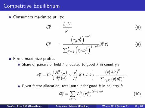
Competitive Equilibrium

Consumers maximize utility:

C 0i =

β0i Yi

p0i(8)

C kji =

(τjip

kj

)−σk

∑Ij ′=1

(τj ′ip

kj ′

)1−σk βki Yi (9)

Firms maximize profits:

Share of parcels of field f allocated to good k in country i :

πfki = Pr

{Afk

i (ω)

Afli (ω)

>pl

i

pki

if l 6= k

}=

(pk

i Afki

)θ∑l∈K

(pl

iAfli

)θ .

Given factor allocation, total output for good k in country i :

Qki =

∑f∈Fi

Afki

(πfk

i

)(θ−1)/θ(10)


Competitive Equilibrium (Continued)

Goods markets clear:

Q0i = C 0

i (11)

Qki =

∑j∈I

τijCkij (12)

Definition

A competitive equilibrium is a set of producer prices, p, output levels, Q,and consumption levels, C, such that Equations (8)-(12) hold

Once CDS (2016) have estimates of parameters (see below) theycompute competitive equilibria for this economy:

at baseline (∼ 2009), to assess model fit and provide model-consistentbenchmark

under the new productivity levels(Afk

i

)′that obtain under climate

change (2071-2100), with full adjustment

under CC but while shutting down various modes of adjustmentStanford Econ 266 (Donaldson) Assignment Models (Empirics) Winter 2016 (lecture 7) 69 / 81

Model Parameter EstimationOverview

Model contains the following unknown parameters:

Preferences: βki and σk

Technology: p0i A0i and θ

Trade costs: τ kij

CDS (2016) estimate these parameters using a cross-section of FAOand GAEZ data from 2009


Estimation ProcedureStep 1: Preferences

Let X kij denote the value of exports of crop k from i to j

With measurement error (ηkij ) in trade flows, Equation (9) implies

lnX kij = E k

i + Mki +

(1− σk

)ln τij + ηk

ij

Estimate σk by OLS treating E ki and Mk

j as fixed effects

For now, set σk = σ for all k = 1...K for simplicity

Finally, use trade and output data to measure expenditure shares:

βki =

∑j 6=i X

kji +

(pk

i Qki −

∑j 6=i X

kij

)GDPi


Estimation ProcedureStep 2: Technology

For crops (k = 1...K ), the GAEZ data provides plausibly unbiasedestimate Afk

i of E[Afk

i (ω)]

= Afki .

CDS (2016) use output and producer price data to estimate θ by NLS:

minθ

∑i ,k 6=0

(ln Qk

i (θ)− lnQki

)2,

where Qki (θ) is output level predicted by model

Qki (θ) =

∑f ∈Fi

Afki

(pk

i Afki

)θ∑

l∈K

(pl

i Afli

)θ

(θ−1)/θ

For outside good they estimate p0i A0i ≡ p0i Q

0i /L

0i from GDP (to

compute p0i Q0i ) and land data (i.e. L0i )


Estimation ProcedureStep 3: Trade Costs

Data on origin-destination price gaps used to estimate τkij

Following a standard free arbitrage argument, for crops andcountry-pairs with positive trade flows, we compute:

ln τkij = ln pk

ij − ln pki

Then assume that for all crops and country-pairs:

ln τkij = α ln dij + εk

ij

Where dij is the great circle distance between major populationcenters (from CEPII ‘gravity’ dataset) and εk

ij is an error term.

Straightforward to extend this method to include a full vector of tradecost determinants (e.g. contiguity, shared language, colonial ties, etc.)

Estimate α by OLS and use α ln dij as our measure of trade costs, ie:

ln τkij = α ln dij


GAEZ Data: Productivity after Climate Change

At baseline:

Climatic conditions obtained from daily weather records, 1961-1990

Agronomic model simulated in each year

Reported Afki is average over these 30 years of runs.

Under climate change:

Exact same agronomic model, just different climatic data. (NB: thismeans that adaptation through technological change, etc is shut down.)

Reported(Afk

i

)′is average over 30 years of agronomic model runs

from 2071-2100

‘Weather’ from 2071-2100 from Hadley CM3 A1F1 global circulationmodel (GCM).

Also allow for CO2 fertilization effect in plants


Other Sources of Data: FAOSTAT, World Bank

From FAOSTAT obtain data on the following (for all countries i andcrops k , in 2009):

Qki , output [tonnes]

pki , producer price [USD/tonne]

L0i , land used by outside good [ha]X k

ij , exports [USD]

pkij , import (cif) price [USD/tonne]

From World Bank obtain data on (for all countries i , in 2009):

p0i Q0i , value of output of outside good [USD]


Estimation Results


Model Fit


Counterfactual Scenarios

Three scenarios (each compared with relevant baseline), designed toillustrate GE mechanisms at work here

Scenario 1:

Climate Change, Trade Costs at Baseline, Full Output Adjustment“True” Impact

Scenario 2:

Climate Change, Trade Costs at Baseline, No Output AdjustmentGains from “Local Specialization” ≡ 6= between 2 and 1

Scenario 3:

Climate Change, Autarky, Full Output AdjustmentGains from “International Specialization” ≡ 6= between 3 and 1


Main Counterfactual simulation results


Main Counterfactual simulation results


Counterfactual simulation results—Robustness


Documents

Lecture 7: Assignment Models (Empirics) - Dave …dave-donaldson.com/.../10/Lecture-7-Assignment-Models-empirics.pdf · { Lecture 7: Assignment Models (Empirics) ... agriculture As