Embed Size (px)
Citation preview

EC400B Math for Micro: Lecture 2
Francesco Nava
September 2013
Nava (LSE) EC400B – Lecture 2 September 2013 1 / 25

Taylor Expansion
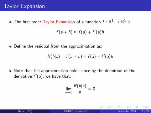
The first order Taylor Expansion of a function f : R1 → R1 is
f (a + h) ≈ f (a) + f ′(a)h
Define the residual from the approximation as:
R(h|a) = f (a + h)− f (a)− f ′(a)h
Note that the approximation holds since by the definition of thederivative f ′(a), we have that:
limh→0
R(h|a)
h= 0
Nava (LSE) EC400B – Lecture 2 September 2013 2 / 25
Taylor Expansion
The first order Taylor Expansion of a function f : R1 → R1 is
f (a + h) ≈ f (a) + f ′(a)h
Define the residual from the approximation as:
R(h|a) = f (a + h)− f (a)− f ′(a)h
Note that the approximation holds since by the definition of thederivative f ′(a), we have that:
limh→0
R(h|a)
h= 0
Nava (LSE) EC400B – Lecture 2 September 2013 2 / 25

Taylor Expansion
Geometrically: this is the formalization of the approximation of thegraph of f (x) by its tangent line at (a, f (a)).
Analytically: it describes the best approximation of f by a polynomialof degree 1.
Nava (LSE) EC400B – Lecture 2 September 2013 3 / 25
Higher Order Taylor Expansions
Definition
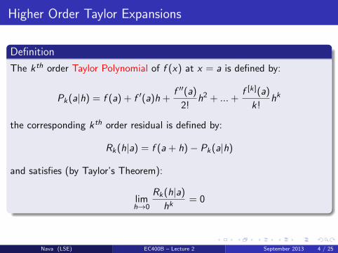
The kth order Taylor Polynomial of f (x) at x = a is defined by:
Pk(a|h) = f (a) + f ′(a)h +f ′′(a)
2!h2 + ... +
f [k](a)
k!hk
the corresponding kth order residual is defined by:
Rk(h|a) = f (a + h)− Pk(a|h)
and satisfies (by Taylor’s Theorem):
limh→0
Rk(h|a)
hk= 0
Nava (LSE) EC400B – Lecture 2 September 2013 4 / 25

A Simple Example
Consider the first and second order Taylor polynomial of theexponential function f (x) = ex at x = 0.
All the derivatives of f (x) at x = 0 equal 1.
Therefore:
P1(0|h) = 1 + h
P2(0|h) = 1 + h +h2
2
For h = 0.2, then:
P1(0|0.2) = 1.2,P2(0|0.2) = 1.22, f (0.2) = 1.22140275816017
Nava (LSE) EC400B – Lecture 2 September 2013 5 / 25

Taylor Expansion for Functions of Several Variables
First Order Taylor Polynomial:
F (a + h) ≈ F (a) +∂F
∂x1(a)h1 + ... +
∂F
∂xn(a)hn
Alternatively, let R1(h|a) denote the residual, to get:
F (a + h) = F (a) + dF (a) · h + R1(h|a)
where dF (a) = (∂F/∂x1, . . . , ∂F/∂xn) is the Jacobian of F at a.
As before R1(h|a)/||h|| → 0 as h→ 0.
Nava (LSE) EC400B – Lecture 2 September 2013 6 / 25

Taylor Expansion for Functions of Several Variables
Second order Taylor Polynomial:
F (a + h) ≈ F (a) + dF (a)h +1
2!hTd2F (a)h
where d2F (a) is the Hessian matrix of F at a:
d2F (a) =
∂2F∂x1∂x1
(a) ... ∂2F∂xn∂x1
(a)
... ... ...∂2F
∂x1∂xn(a) ... ∂2F
∂xn∂xn(a)
The extension for order k then trivially follows.
Nava (LSE) EC400B – Lecture 2 September 2013 7 / 25

Definition Extreme Points
Definition
The ball B(x, ε) centred at x of radius ε is the set of all vectors y in Rn
whose distance from x is less than ε:
B(x, ε) = {y ∈ Rn|ε > ||y − x||}
Definition
Let f (x) be a real valued function defined on a subset C of Rn.A point x∗ in C is:
a global maximizer for f (x) on C if
f (x∗) ≥ f (x) for all x ∈ C
a strict global maximizer for f (x) on C if
f (x∗) > f (x) for all x ∈ C such that x 6= x∗
Nava (LSE) EC400B – Lecture 2 September 2013 8 / 25

Definition Extreme Points
Definition
Let f (x) be a real valued function defined on a subset C of Rn.A point x∗ in C is:
a local maximizer for f (x) if ε > 0 exists such that:
f (x∗) ≥ f (x) for all x ∈ C ∩ B(x∗, ε)
a strict local maximizer for f (x) if ε > 0 exists such that:
f (x∗) > f (x) for all x ∈ C ∩ B(x∗, ε) such that x 6= x∗
a critical point for f (x) if first partial derivatives exist at x∗ and if:
∂f (x∗)
∂xi= 0 for i = 1, 2, ..., n ⇔ df (x∗) = 0
Nava (LSE) EC400B – Lecture 2 September 2013 9 / 25
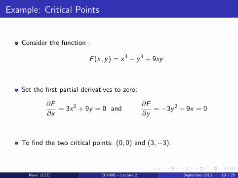
Example: Critical Points
Consider the function :
F (x , y) = x3 − y3 + 9xy
Set the first partial derivatives to zero:
∂F
∂x= 3x2 + 9y = 0 and
∂F
∂y= −3y2 + 9x = 0
To find the two critical points: (0, 0) and (3,−3).
Nava (LSE) EC400B – Lecture 2 September 2013 10 / 25
Do Extreme Points Exist?
Theorem (Extreme Value Theorem)
Let C be a compact (closed and bounded) subset of Rn.
Let f (x) be a continuous function defined on C.
If so, there exists a point x∗ in C , which is a global maximizer of f ,and there exists a point x∗ in C , which is a global minimizer of f .
That is:f (x∗) ≤ f (x) ≤ f (x∗) for all x ∈ C
Nava (LSE) EC400B – Lecture 2 September 2013 11 / 25

Functions of One Variable: FOC
First Order Necessary Conditions for a maximum in R :
Let f (x) be a continuous differentiable function on an interval I .
If x∗ is a local maximizer of f (x) then:
either x∗ is an end point of I
or f ′(x∗) = 0
Nava (LSE) EC400B – Lecture 2 September 2013 12 / 25

Functions of One Variable: SOC
Second Order Sufficient Conditions for a maximum in R:
Suppose that f (x), f ′(x), f ′′(x) are all continuous on an interval in I andthat x∗ is a critical point of f (x) then:
if f ′′(x) ≤ 0 for all x ∈ I , then x∗ is a global maximizer of f (x) on I .
if f ′′(x) < 0 for all x ∈ I such that x 6= x∗, then x∗ is a strict globalmaximizer of f (x) on I .
if f ′′(x∗) < 0, then x∗ is a strict local maximizer of f (x) on I .
Nava (LSE) EC400B – Lecture 2 September 2013 13 / 25
Functions of Several Variables: FOC
First Order Necessary Conditions for a maximum in Rn:
Let f (x) be a continuous real valued function for which all first partialderivatives exist and are continuous on a subset C ⊂ Rn.
If x∗ is both an interior point of C and a local maximizer of f (x), then x∗
is a critical point of f (x), that is:
∂f (x∗)
∂xi= 0 for i = 1, 2, ..., n
Nava (LSE) EC400B – Lecture 2 September 2013 14 / 25
Functions of Several Variables: SOC
How can we determine whether a critical point is a local maximum ora local minimum in this more general setup?
To this end we have to consider the Hessian of the map f(ie the matrix of the second order partial derivatives).
Note that the Hessian is always a symmetric matrix, sincecross-partial derivatives are equal (Clairaut-Schwarz Theorem).
Nava (LSE) EC400B – Lecture 2 September 2013 15 / 25

Functions of Several Variables: SOC
Second Order Sufficient Conditions for a local maximum in Rn
Let f (x) be a continuous real valued function for which all first and secondpartial derivatives exist and are continuous on a subset C ⊂ Rn.
If x∗ is critical point of f then:
if d2f (x∗) is negative definite, x∗ is a strict local maximizer of f .
if d2f (x∗) is positive definite, x∗ is a strict local minimizer of f .
Nava (LSE) EC400B – Lecture 2 September 2013 16 / 25

Functions of Several Variables: SOC
It is also true that if x∗ is an interior point and:
a global maximum of f , then d2f (x∗) is negative semidefinite.
a global minimum of f , then d2f (x∗) is positive semidefinite.
But, it is not true that if x∗ is a critical point and d2f (x∗) is negative(positive) semidefinite, then x∗ is a local maximum (minimum).
A counterexample is f (x) = x3:
which has a critical point at x = 0
in which d2f (0) = 0 is semidefinite.
But x = 0 is not a maximum or minimum, it’s a saddle point.
Nava (LSE) EC400B – Lecture 2 September 2013 17 / 25

Back to the Example
Consider again F (x , y) = x3 − y3 + 9xy . The Hessian satisfies:
d2F (x , y) =
(6x 99 −6y
)The first order leading principle minor is 6x andthe second order leading principal minor is −36xy − 81.
At (0, 0) the two minors are 0 and −81.Hence the Hessian is indefinite and(0, 0) is not an extreme point, it is a saddle point.
At (3,−3) these two minors are positive.Hence, (3,−3) is a strict local minimum of F .
However, (3,−3) is not a global minimum of F(to see why this is the case consider (x , y)→ (0, inf)).
Nava (LSE) EC400B – Lecture 2 September 2013 18 / 25

Sketch of the Proof
Consider the Taylor Expansion:
F (x∗ + h) = F (x∗) + dF (x∗)h +1
2hTd2F (x∗)h + R(h)
Ignore R(h), set dF (x∗) = 0, and observe that:
F (x∗ + h)− F (x∗) ≈ 1
2hTd2F (x∗)h
If d2F (x∗) is negative definite, then for all small enough h 6= 0, the righthand side is negative.
This in turn implies that for small enough h:
F (x∗ + h) < F (x∗)
Hence, x∗ is a strict local maximizer of F .
Nava (LSE) EC400B – Lecture 2 September 2013 19 / 25

Concavity and Convexity
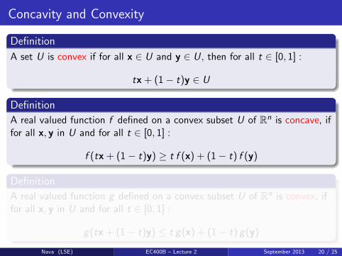
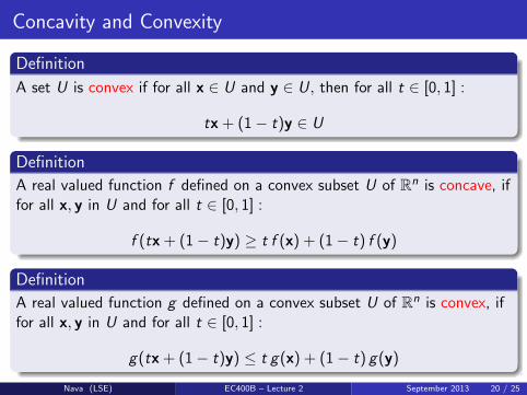
Definition
A set U is convex if for all x ∈ U and y ∈ U, then for all t ∈ [0, 1] :
tx + (1− t)y ∈ U
Definition
A real valued function f defined on a convex subset U of Rn is concave, iffor all x, y in U and for all t ∈ [0, 1] :
f (tx + (1− t)y) ≥ t f (x) + (1− t) f (y)
Definition
A real valued function g defined on a convex subset U of Rn is convex, iffor all x, y in U and for all t ∈ [0, 1] :
g(tx + (1− t)y) ≤ t g(x) + (1− t) g(y)
Nava (LSE) EC400B – Lecture 2 September 2013 20 / 25
Concavity and Convexity
Definition
A set U is convex if for all x ∈ U and y ∈ U, then for all t ∈ [0, 1] :
tx + (1− t)y ∈ U
Definition
A real valued function f defined on a convex subset U of Rn is concave, iffor all x, y in U and for all t ∈ [0, 1] :
f (tx + (1− t)y) ≥ t f (x) + (1− t) f (y)
Definition
A real valued function g defined on a convex subset U of Rn is convex, iffor all x, y in U and for all t ∈ [0, 1] :
g(tx + (1− t)y) ≤ t g(x) + (1− t) g(y)
Nava (LSE) EC400B – Lecture 2 September 2013 20 / 25

Concavity and Convexity
Observations:
f is concave if and only if −f is convex.
linear functions are convex and concave.
concave and convex functions must to have convex sets as theirdomains for the definitions to apply.
Theorem
Let f be a continuous differentiable function on a convex subset U of Rn.
If so, f is concave on U if and only if for all x, y in U:
f (y)− f (x) ≤ df (x) (y − x) =
=∂f (x)
∂x1(y1 − x1) + ... +
∂f (x)
∂xn(yn − xn)
Nava (LSE) EC400B – Lecture 2 September 2013 21 / 25

Proof for R1
Since f is concave, then
t f (y) + (1− t) f (x) ≤ f (ty + (1− t)x)⇔f (x) + t(f (y)− f (x)) ≤ f (x + t(y − x))⇔
f (y)− f (x) ≤ f (x + t(y − x))− f (x)
t⇔
f (y)− f (x) ≤ f (x + h)− f (x)
h(y − x)
where the latter holds for h = t(y − x).
The limit the last expression when h→ 0 gives:
f (y)− f (x) ≤ f ′(x)(y − x)
Nava (LSE) EC400B – Lecture 2 September 2013 22 / 25
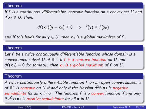
Theorem
If f is a continuous, differentiable, concave function on a convex set U andif x0 ∈ U, then:
df (x0)(y − x0) ≤ 0 ⇒ f (y) ≤ f (x0)
and if this holds for all y ∈ U, then x0 is a global maximizer of f .
Theorem
Let f be a twice continuously differentiable function whose domain is aconvex open subset U of Rn. If f is a concave function on U anddf (x0) = 0 for some x0, then x0 is a global maximum of f on U.
Theorem
A twice continuously differentiable function f on an open convex subset Uof Rn is concave on U if and only if the Hessian d2f (x) is negativesemidefinite for all x in U. The function f is a convex function if and onlyif d2f (x) is positive semidefinite for all x in U.
Nava (LSE) EC400B – Lecture 2 September 2013 23 / 25
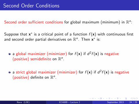
Second Order Conditions
Second order sufficient conditions for global maximum (minimum) in Rn:
Suppose that x∗ is a critical point of a function f (x) with continuous firstand second order partial derivatives on Rn. Then x∗ is:
a global maximizer (minimizer) for f (x) if d2f (x) is negative(positive) semidefinite on Rn.
a strict global maximizer (minimizer) for f (x) if d2f (x) is negative(positive) definite on Rn.
Nava (LSE) EC400B – Lecture 2 September 2013 24 / 25

Why Care about Concavity?
The property that critical points of concave functions are globalmaximizers is an important one in economic theory.
For example, many economic principles, such as marginal rate ofsubstitution equals the price ratio, or marginal revenue equalsmarginal cost are simply the first order necessary conditions of thecorresponding maximization problems (as we will see).
Ideally, such conditions should also be sufficient to identify optimizingbehavior. But this will indeed be the case when the objectivefunctions are concave.
Nava (LSE) EC400B – Lecture 2 September 2013 25 / 25