Efficient Lie-Poisson Integrator for Secular Spin Dynamics of Rigid Bodies

SÃlawomir Breiter

Astronomical Observatory, Adam Mickiewicz University, SÃloneczna 36, PL 60-286 Poznan,Poland

breiter@amu.edu.pl

David Nesvorny

Southwest Research Institute, 1050 Walnut St., Suite 400, Boulder, CO 80302, USA

davidn@boulder.swri.edu

and

David Vokrouhlicky

Institute of Astronomy, Charles University, V Holesovickach 2, 180 00 Prague 8, Czech Republic

vokrouhl@cesnet.cz

ABSTRACT

A fast and efficient numerical integration algorithm is presented for the problemof the secular evolution of the spin axis. Under the assumption that a celestial bodyrotates around its maximum moment of inertia, the equations of motion are reduced tothe Hamiltonian form with a Lie-Poisson bracket. The integration method is based onthe splitting of the Hamiltonian function and so it conserves the Lie-Poisson structure.Two alternative partitions of the Hamiltonian are investigated and second order leapfrogintegrators are provided for both cases. Non-Hamiltonian torques can be incorporatedinto the integrators with a combination of Euler and Lie-Euler approximations. Numer-ical tests of the methods confirm their good properties resulting in short computationtime and reliability on long integration intervals.

Subject headings: methods: numerical — solar system: general — celestial mechanics

1. Introduction

Motion of celestial bodies is conventionally split into translation of the center of mass androtation about the proper spin axis (Whittaker 1944). Planetary dynamics offers a plethora ofcases where translation and rotation motion interact via resonant phenomena. This manifests

– 2 –

mainly through the translation mode affecting the rotation mode, in either (or both) of the twocases:

1. Rotation about the spin axis resonates with orbital motion, such as the case of spin-orbitcoupling of close planetary satellites, Mercury or secondary components of asteroid binaries.

2. Precession of the spin axis resonates with precession of the orbital plane, such as the caseof a number of planetary satellites (including our Moon), some terrestrial planets, possiblySaturn, and many asteroids.

It has been long understood that occurrence of these resonant states reflects in many cases thepast evolution of the spin and/or orbit due to dissipative effects. An accurate modeling of theseevolutionary paths is a very interesting goal in planetary science. However, such ambitious modelsoften depend on a number of unknown parameters, related to non-gravitational torques, and aresensitive to a chaotic nature of the orbital evolution of gravitationally interacting bodies. As aresult, efficient numerical tools are often very useful to sample a wide range of parameters withina reasonable amount of CPU time.

In this paper, we develop an efficient integrator to tackle the problems in planetary dynamicslike those described in item 2. As far as the problems of major planets are concerned, the rotationhistory of Mercury and Venus is a type 1 problem (Peale 1969, 1974; Goldreich & Peale 1970;Ward & de Campli 1979), but on the other hand Earth and Mars remain the distinguished caseswhere secular spin dynamics (type 2) applies. The basic framework for this case was establishedin the classical paper by Colombo (1966), but the complications for Earth and Mars arise dueto the necessity of accurate representation of the orbital evolution and its influence on the spinhistory. Ward (1973, 1974, 1979) was the first to discover large-scale oscillations in Mars’ obliquityresponding to forcing torques due to orbital evolution, itself driven by planetary perturbations.This field has been later mastered by Laskar and collaborators using steadily improved solutions ofplanetary motion (e.g. Laskar & Robutel 1993). Additional difficulty in understanding planetaryspin evolution is due to long-term effects of non-gravitational torques, such as tides (Peale 1974;Ward 1975, 1980; Neron de Surgy & Laskar 1997), core-mantle friction (Rochester 1976) and/oratmospheric torques (Dobrovolskis & Ingersoll 1980; Dobrovolskis 1980; Correia & Laskar 2001,2003; Correia et al. 2003). Modern paleoclimate studies for both Earth and Mars rely on thesecomplicated models (Laskar et al. 2002, 2004a,b). In addition, Ward & Hamilton (2004), andHamilton & Ward (2004), have recently brought an attractive model for explaining Saturn’s largeobliquity as a result of a resonance torque due to Neptune-raised terms in Saturn’s orbital motionmodulated, on a long-term, by a dissipating planetesimal disc. And not only the Solar Systemplanets are the subject of such studies. The growing interest in testing newly discovered planetarysystems for habitable climate conditions also calls for an efficient obliquity tracking tool (Atobeet al. 2004).

– 3 –

In the realm of minor bodies (natural and artificial satellites, asteroids, and comets) resonantinteractions of the orbital plane precession with the spin axis is so widely studied that any attemptof brief bibliographic guide is doomed to be unsatisfactory. Here we only briefly touch asteroidapplications stemming from the work of Skoglov (1997, 1999). Wider publicity to this field has beengot after Vokrouhlicky et al. (2003) solved, using a combination of secular spin-orbit resonant lockingand the long-term influence of the thermal torques (Rubincam 2000; Vokrouhlicky & Capek 2002),the puzzling alignment of spin axes for five Koronis family member asteroids (Slivan 2002). Manymore asteroids, especially those with low-inclination orbits and in the inner part of the main belt,are expected to reside in similar spin-orbit resonances (Rubincam et al. 2002). Intermittent resonantstates are also expected for near-Earth asteroids, such as in the case of (433) Eros (Vokrouhlickyet al. 2005). Growing knowledge of spin states for small near-Earth (and main-belt) asteroids,that will likely undergo a spectacular leap after data from future space-born missions are available(e.g. Kaasalainen 2004), will soon allow statistical studies of obliquity distribution across a widerange of sizes. Understanding the long-term (secular) dynamics of asteroid spin axes will becomea necessary prerequisite to interpret these data.

Such is the motivation for a development of an efficient numerical integration tool that mayhelp in further studies of the above mentioned problems. There exists a general purpose Lie-Poissonintegrator, developed by Touma & Wisdom (1994a), that handles the complete translation-rotationproblem, but it involves a costly “Keplerian drift” part that can be suppressed under few simpli-fying assumptions. Assuming principal axis rotation and averaging the appropriate Newton-Eulerequations over orbital periods we achieve a considerable gain in the computational efficiency. Post-poning individual planetary applications to the forthcoming work, we aim at presenting numericaltools developed and optimized for this particular task.

In Sec. 2 we review the mathematical formulations of the secular spin dynamics for a rigidbody in orbit about a force center and bring the underlying equations into a Hamiltonian formthat allows application of Lie-Poisson splitting methods. In Sec. 3 we construct two alternativeLie-Poisson integrators based upon different Hamiltonian splitting. The elementary maps can beused as building blocks for a high order integrator, but we focus on the second order “leapfrog”algorithm as the most convenient one. In Sec. 4 we extend our previous formulation, accountingfor gravitational torques only, to the case when arbitrary (dissipative) torques are required. InSec. 5 we test the properties of the second-order “leapfrog” implementation for the secular spinaxis evolution.

2. Lie-Poisson equations of rotation

2.1. Equations of motion in an inertial frame

In order to study the long-term evolution of the spin axis, we begin with averaged Newton-Euler equations describing the evolution of the unitary spin direction vector e under the action of

– 4 –

the mean Solar torque.1 The torque is perpendicular to the unitary vector Np, the latter beingnormal to the orbital plane. Let us assume that the body rotates around the principal axis of theinertia tensor. In an arbitrary inertial reference frame, say Ecliptic-Equinox of some epoch, it holds(Bertotti et al. 2003,p. 176)

de

dt= e× α (Np · e) Np, (1)

whereα(t) =

3µ∆2ωr a3 η3

, (2)

is a function of the heliocentric gravitation parameter µ (gravity constant times the total mass of thesystem), dynamical ellipticity ∆ defined in terms of the principal moments of inertia I1 ≤ I2 ≤ I3

as

∆ =I3 − 1

2(I1 + I2)I3

, (3)

the mean rotation frequency ωr, and two time-dependent orbital elements: major semi-axis a andeccentricity e via η =

√1− e2.

The time dependence of α is the result of planetary perturbations in a and η. The orientationof the unit vector Np, normal to the orbital plane, is also time-dependent due to perturbationsin inclination I and in the longitude of the ascending node Ω. If the body possesses a close ora distant satellite, one can recalibrate the ellipticity ∆ to include information about the averagesolar torque exerted on the satellite orbit similarly to Neron de Surgy & Laskar (1997) or Ward &Hamilton (2004).

Equation (1) can be reformulated in the Lie-Poisson formalism that reveals its Hamiltonian,although non-canonical, structure (Olver 1993; Touma & Wisdom 1994a). Let us introduce twooperators: Q : R3 → so(3), and q : so(3) → R3 acting between the R3 Euclidian space and theso(3) Lie algebra of skew-symmetric matrices. For any vector v ∈ R3, Q(v) is a skew symmetricmatrix

Q(v) =

0 −v3 v2

v3 0 −v1

−v2 v1 0

. (4)

On the other hand, given a skew-symmetric matrix V = [V ]ij ∈ so(3), we define

q(V) = (V32, V13, V21)T. (5)

These operators link the vector product and the matrix product. Given any pair of vectors v, w

v ×w = Q(v)w, (6)

1For definiteness, we speak about an asteroid in orbit about the Sun. However, the same approach applies to a

planet, or a satellite in orbit about a planet, etc.

– 5 –

and for any skew-symmetric matrix V

Vw = q(V)×w. (7)

Equation (1) can be rewritten as

de

dt= Q(e)

(∂H∂e

)T

, (8)

whereH(e, t) =

α

2(Np · e)2 , (9)

and we use the convention of Battin (1987), i.e. for f ∈ R, the derivative ∂f∂e is a row vector

( ∂f∂e1

, ∂f∂e2

, ∂f∂e3

), dual to the usual column vector.

Let us now introduce a bilinear, skew-symmetric differential operator

f ; g =∂f

∂eQ(e)

(∂g

∂e

)T

. (10)

Checking that ; satisfies the Jacobi identity

f ; g; h+ g; h; f+ h; f; g = 0, (11)

and observing the linearity of Qij with respect to the components of e, we identify Eq. (10) asthe definition of a Lie-Poisson bracket (Olver 1993). Accordingly, equations of motion (8) areHamiltonian (but not canonical)

de

dt= e;H , (12)

with the Hamiltonian function H. Note that for any scalar function g,

e · e; g = 0, (13)

hence all solutions of Eqs. (12), regardless of the actual form of the Hamiltonian function, belongto the SO(3) group of rotations, respecting the e2

1 + e22 + e2

3 = 1 constraint.

In the Ecliptic-Equinox inertial frame, Np can be parameterized by means of orbital inclinationI and longitude of the ascending node Ω. The transformation of any vector r from the inertialframe to the nodal-orbital frame, where it becomes r′ = Mr, is defined by the rotation matrix

M = R1(I)R3(Ω) = (14)

=

cosΩ sin Ω 0− cos I sinΩ cos I cosΩ sin I

sin I sinΩ − sin I cosΩ cos I

.

– 6 –

Because N ′p = (0, 0, 1)T, we find

Np = MTN ′p =

sin I sinΩ− sin I cosΩ

cos I

=

=

2 p√

1− q2 − p2

−2 q√

1− q2 − p2

1− 2 (q2 + p2)

. (15)

In the latter form, we used nonsingular elements

q + i p = sin (I/2) exp iΩ. (16)

Thus we can write explicitly the Hamiltonian as:

H(e, t) =α

2((e1 sinΩ− e2 cos Ω) sin I + e3 cos I)2 . (17)

In the absence of planetary perturbations α, Ω, and I are constant, and we obtain the integral ofmotion H = const.

2.2. Transformation of reference frame

The Hamiltonian (17) can be simplified by an appropriate rotation of the reference frame.But will an orthogonal (and possibly time-dependent) transformation of variables conserve theHamiltonian structure of equations (12) ? More precisely, there are two questions to be answered:is the Lie-Poisson bracket invariant with respect to orthogonal transformations, and what kind ofremainder should be added to the Hamiltonian if the transformation is time-dependent.

Let e′ = P(t) e, where P ∈ SO(3) is an arbitrary rotation matrix. For any pair of scalarfunctions f , g, their Lie-Poisson bracket (10) transforms as follows

f ; g =∂f

∂eQ(e)

(∂g

∂e

)T

=

=∂f

∂e′∂e′

∂e

[PTe′ ×

(∂g

∂e′∂e′

∂e

)T]

=

=∂f

∂e′P

[PTe′ ×

(∂g

∂e′P

)T]

=

=∂f

∂e′PPT detP

[e′ ×

(∂g

∂e′

)T]

=

=∂f

∂e′Q(e′)

(∂g

∂e′

)T

. (18)

– 7 –

Thus we have demonstrated that the Lie-Poisson bracket (10) is invariant with respect to rotations,hence we can substitute e = PT(t)e′ into Eq. (12), obtaining

d(PTe′)dt

=PTe′;H

, (19)

where the Lie-Poisson bracket is evaluated with respect to e′ as in Eq. (18). After elementarytransformations

de′

dt=

e′;H−PPTe′. (20)

From the properties of rotation matrices, we know that PPT is a skew-symmetric matrix, and

q(PPT) = ω, (21)

where ω is the angular rate vector of the rotating reference frame. This allows us to rewriteequations of motion as

de′

dt=

e′;H

+ e′ × ω. (22)

Bute′ × ω = Q(e′)ω =

e′;ω · e′ , (23)

hence, from the linearity of Lie-Poisson brackets we obtain the Hamiltonian equations of motion ina rotating frame

de′

dt=

e′;H′ , (24)

whereH′(e′, t) = H(PTe′, t) + ω · e′. (25)

2.3. Asteroid spin axis in orbital frame

Let us adopt the orbital reference frame defined by orthonormal vectors i′, j′,k′, where k′ isnormal to the osculating orbital plane. Then, the Hamiltonian function (25), where H is given byEq. (9), takes form

H′ = α(t)2

(e′3

)2 + ω1(t) e′1 + ω2(t) e′2 + ω3(t) e′3. (26)

Directing i′ towards the ascending node of the orbit may sometimes be preferred, but usuallythis is not the best choice. It is much more convenient to rotate i′ backwards, by an angle −Ωalong the orbital plane. The gain is twofold: not only do we avoid problems of undefined nodeswhen sin I = 0, but we also partially compensate the reference frame motion due to Ω when theinclination is small.

Let us use the symbol v to stand for the spin vector e′ in this particular reference frame. Itscomponents will be v = (x, y, z)T. Hence, the transformation to the new reference frame is v = Pe,where

P = R3(−Ω)R1(I)R3(Ω), (27)

– 8 –

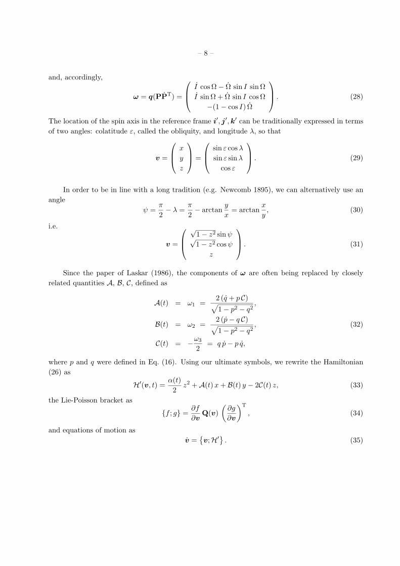
and, accordingly,

ω = q(PPT) =

I cosΩ− Ω sin I sin ΩI sinΩ + Ω sin I cosΩ

−(1− cos I) Ω

. (28)

The location of the spin axis in the reference frame i′, j′, k′ can be traditionally expressed in termsof two angles: colatitude ε, called the obliquity, and longitude λ, so that

v =

x

y

z

=

sin ε cosλ

sin ε sinλ

cos ε

. (29)

In order to be in line with a long tradition (e.g. Newcomb 1895), we can alternatively use anangle

ψ =π

2− λ =

π

2− arctan

y

x= arctan

x

y, (30)

i.e.

v =

√1− z2 sinψ√1− z2 cosψ

z

. (31)

Since the paper of Laskar (1986), the components of ω are often being replaced by closelyrelated quantities A, B, C, defined as

A(t) = ω1 =2 (q + p C)√1− p2 − q2

,

B(t) = ω2 =2 (p− q C)√1− p2 − q2

, (32)

C(t) = −ω3

2= q p− p q,

where p and q were defined in Eq. (16). Using our ultimate symbols, we rewrite the Hamiltonian(26) as

H′(v, t) =α(t)2

z2 +A(t) x + B(t) y − 2C(t) z, (33)

the Lie-Poisson bracket as

f ; g =∂f

∂vQ(v)

(∂g

∂v

)T

, (34)

and equations of motion asv =

v;H′ . (35)

– 9 –

2.4. Reduction to the canonical form

Our equations of motion are locally equivalent with the canonical form given by Laskar &Robutel (1993). Let us exclude the poles z = ±1 and introduce two variables on the surface of thesphere v2 = 1: a longitude related ψ from Eq. (30) and some unspecified function of colatitude X(ε).Under the new parametrization h = (ψ, X)T, the Lie-Poisson bracket f ; g will be transformedinto a reduced operator (f ; g), according to the transformation rule (Olver 1993)

(f ; g) =(

∂f

∂h

)(ψ; ψ ψ; XX; ψ X; X

)(∂g

∂h

)T

,

i.e.

(f ; g) =∂X

∂z

(∂f

∂ψ

∂g

∂X− ∂f

∂X

∂g

∂ψ

). (36)

Thus an obvious choice X = z = cos ε brings in the classical, canonically conjugate pair ψ, X

and the canonical Poisson bracket (ψ; X) = 1. Using our Hamiltonian (33) expressed in terms ofcanonical variables

H′ =α(t)2

X2 − 2C(t) X + (37)

+√

1−X2 (A(t) sinψ + B(t) cos ψ) ,

we obtain the canonical equations of Laskar & Robutel (1993)

X = (X;H′) = −∂H′∂ψ

=

=√

1−X2 (−A cosψ + B sinψ) , (38)

ψ = (ψ;H′) =∂H′∂X

=

= α X − 2 C − X√1−X2

(A sinψ + B cosψ) .

The canonical equations of motion are only two, as compared to three components of v, but theypossess serious drawbacks: singularities at X2 = 1 and a more complicated form.

2.5. Extended phase space

Introducing an additional canonically conjugate pair of variables u,E, we can replace a time-dependent Hamiltonian H′(v, t) from Eq. (33) with a new, conservative function K of five variablesw = (x, y, z, E, u)

K(w) = H′(v, u) + E =α(u)

2z2 +A(u) x +

+B(u) y − 2 C(u) z + E = const, (39)

– 10 –

where α, A, B, C become functions of the formal, time-like u. In the extended phase space theLie-Poisson bracket (34) can be replaced by

f ; g =∂f

∂wJ(v)

(∂g

∂w

)T

, (40)

where the structure matrix J is

J(v) =

0 −z y 0 0z 0 −x 0 0−y x 0 0 00 0 0 0 −10 0 0 1 0

. (41)

The equations of motion in the extended phase space are w = w;K, or explicitly

x = α(u) z y − 2 C(u) y − B(u) z,

y = −α(u) z x + 2 C(u)x +A(u) z,

z = −A(u) y + B(u) x, (42)

E = −z2

2dα

du− x

dAdu

− ydBdu

+ 2 zdCdu

,

u = 1.

These last equations deserve a few comments. First we note that t and u differ only by an arbitraryadditive constant, with u = t as the most natural choice. The evolution of the energy-like variableE counterbalances the varying H′ in order to provide the constant K. As a matter of fact, one maysolve the equations for v without any knowledge of the values of E. Thus we will not pay attentionto the evolution of this “variable-in-being”.

3. Explicit Lie-Poisson integrators

According to the principles of the so-called “splitting method” (McLachlan & Quispel 2002),an explicit integrator can be built as a composition of solutions to the equations of motion generatedby separate terms of a partitioned Hamiltonian. We consider two ways of splitting K that differonly by the placement of the E variable. Surprisingly, the two resulting algorithms are completelydifferent.

3.1. Three-terms splitting method (LP3)

The first integration algorithm results if we identify three different, noncommuting terms ofthe Hamiltonian

K(w) = K0(E) +K1(z, u) +K2(v, u), (43)

– 11 –

where

K0 = E, (44)

K1 =α(u)

2z2, (45)

K2 = A(u) x + B(u) y − 2C(u) z. (46)

Each Kj generates the Lie-Poisson equations of motion

w = w;Kj ≡ Ljw, (47)

that can be solved explicitly. The solutions will be formally represented by means of the operatorsΨj,τ = exp (τLj) that map initial conditions w(t) onto

w(t + τ) = Ψj,τw(t) = exp (τLj)w(t). (48)

The flow generated by K0 is quite trivial. The equations of motion w = L0w, or

v = 0, E = 0, u = 1, (49)

amount to a simple propagation of the formal time u

Ψ0,τv = v, Ψ0,τu = u + τ, Ψ0,τE = E. (50)

Note that the remaining terms K1 and K2 will not contain E, hence the value of u will be fixed innext two flows.

The K1 term consists of a monomial z2 times a constant. Accordingly, the equations of motionw = L1w should describe rotation around z axis with the rate depending on αz, which is indeedthe case. The physics behind

x = α(u) z y,

y = −α(u)z x,

z = 0,

E = −dα(u)du

z2

2 ,

u = 0,

(51)

is clear: a regular precession of the spin axis forced by the mean solar torque that vanishes if ε = 12π

(i.e. z = 0). Solving Eqs. (51) we obtain a non-linear map for v

Ψ1,τv =

cosϕ1 sinϕ1 0− sinϕ1 cosϕ1 0

0 0 1

v, (52)

with ϕ1 = α(u) z τ , andΨ1,τu = u. (53)

– 12 –

The knowledge of Ψ1,τE is not required.

Equations of motion w = L2w, generated by the last term K2, are linear. For v they representthe effect of inertial forces due to the planetary perturbations of the reference frame. Recall thatu is fixed, so the reference frame rotates with a constant rate. Thus, for v

v =

0 −2C(u) −B(u)2C(u) 0 A(u)B(u) −A(u) 0

v = −ω × v. (54)

The solution of (54) isΨ2,τv = ω−2 Mv, (55)

with the following elements of matrix M

M11 = A2 +(B2 + 4C2

)cos (ωτ),

M12 = 2AB sin2(ωτ/2)− 2Cω sin (ωτ),

M13 = −4AC sin2(ωτ/2)− Bω sin (ωτ),

M21 = 2AB sin2(ωτ/2) + 2Cω sin (ωτ),

M22 = B2 +(A2 + 4C2

)cos (ωτ), (56)

M23 = −4BC sin2(ωτ/2) +Aω sin (ωτ),

M31 = −4AC sin2(ωτ/2) + Bω sin (ωτ),

M32 = −4BC sin2(ωτ/2)−Aω sin (ωτ),

M33 = 4C2 +(A2 + B2

)cos (ωτ),

andω =

√A2 + B2 + 4C2. (57)

For the remaining two variables

E = −v · dω

du, u = 0, (58)

soΨ2,τu = u, (59)

and, as usually, we pay no attention to the value of E.

Knowing the explicit form of each Lj generated flow, we can approximate the solution ofEqs. (42) on the stepsize interval h, composing the Ψj,βkh maps with appropriate step subdivisionconstants βk. The basic, first-order approximation is obtained as

w(t + h) = Ψ2,h Ψ1,h Ψ0,h w(t) + O(h2

). (60)

Throughout the paper, any composition of Ψ0, Ψ1, and Ψ2 maps will be referred to as an LP3integrator.

– 13 –

3.2. Two-terms splitting method (LP2)

Intuitively, one might think that freezing the rates of the reference frame motion, effected byisolating E from the remaining terms of K, should produce the simplest algorithm. It is not so,however. Let us join K0 and K2 into a single term K20, so that we have

K = K1 +K20, (61)

where

K1 =α(u)

2z2, (62)

K20 = A(u) x + B(u) y − 2C(u) z + E =

= ω(u) · v + E. (63)

There is no need to repeat the discussion of w = L1w, because the operator Ψ1,τ has alreadybeen presented in Eqs. (52) and (53). The second term leads to w = L20w, that is

v = v × ω, (64)

E = −v · dω

du= −v · ω, (65)

u = 1. (66)

Equations (54) and (64), or (58) and (65) may look similar at the first glimpse, but it is u = 1 thatmakes the difference and leads to dω

du = ω. The best way to solve Eq. (64) is to think about itsphysics. It describes the constant e referred to an inertial frame as seen in the noninertial referenceframe i′, j′, k′. In other words,

Ψ20,τv = M20 v, (67)

where M20 is the matrix of rotation to the inertial frame at the initial t = u, and then back to theorbital frame at u + τ . In terms of Ω0 = Ω(u), Ω1 = Ω(u + τ), I0 = I(u), and I1 = I(u + τ)

M20 = R3(−Ω1)R1(I1)R3(Ω1 − Ω0)

R1(−I0)R3(Ω0). (68)

It is better, however, to use the nonsingular elements q0, p0 and q1, p1. If

R(q, p) =

1− 2 p2 2 q p 2 p ν

2 q p 1− 2 q2 −2 q ν

−2 p ν 2 q ν 2 ν2 − 1

, (69)

where ν =√

1− q2 − p2, then

M20 = [R(q1, p1)]T R(q0, p0). (70)

– 14 –

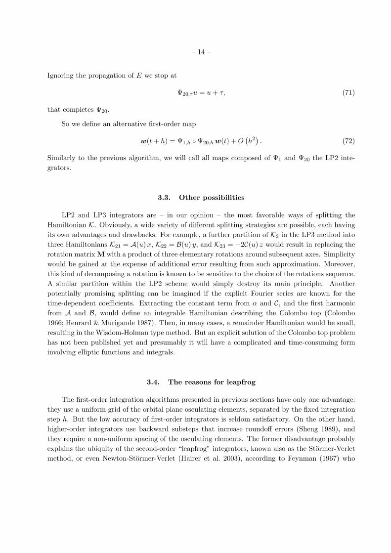
Ignoring the propagation of E we stop at

Ψ20,τu = u + τ, (71)

that completes Ψ20.

So we define an alternative first-order map

w(t + h) = Ψ1,h Ψ20,h w(t) + O(h2

). (72)

Similarly to the previous algorithm, we will call all maps composed of Ψ1 and Ψ20 the LP2 inte-grators.

3.3. Other possibilities

LP2 and LP3 integrators are – in our opinion – the most favorable ways of splitting theHamiltonian K. Obviously, a wide variety of different splitting strategies are possible, each havingits own advantages and drawbacks. For example, a further partition of K2 in the LP3 method intothree Hamiltonians K21 = A(u) x, K22 = B(u) y, and K23 = −2C(u) z would result in replacing therotation matrix M with a product of three elementary rotations around subsequent axes. Simplicitywould be gained at the expense of additional error resulting from such approximation. Moreover,this kind of decomposing a rotation is known to be sensitive to the choice of the rotations sequence.A similar partition within the LP2 scheme would simply destroy its main principle. Anotherpotentially promising splitting can be imagined if the explicit Fourier series are known for thetime-dependent coefficients. Extracting the constant term from α and C, and the first harmonicfrom A and B, would define an integrable Hamiltonian describing the Colombo top (Colombo1966; Henrard & Murigande 1987). Then, in many cases, a remainder Hamiltonian would be small,resulting in the Wisdom-Holman type method. But an explicit solution of the Colombo top problemhas not been published yet and presumably it will have a complicated and time-consuming forminvolving elliptic functions and integrals.

3.4. The reasons for leapfrog

The first-order integration algorithms presented in previous sections have only one advantage:they use a uniform grid of the orbital plane osculating elements, separated by the fixed integrationstep h. But the low accuracy of first-order integrators is seldom satisfactory. On the other hand,higher-order integrators use backward substeps that increase roundoff errors (Sheng 1989), andthey require a non-uniform spacing of the osculating elements. The former disadvantage probablyexplains the ubiquity of the second-order “leapfrog” integrators, known also as the Stormer-Verletmethod, or even Newton-Stormer-Verlet (Hairer et al. 2003), according to Feynman (1967) who

– 15 –

discovered this algorithm in Isaac Newton’s Principia. The leapfrog uses only the forward, uni-formly spaced substeps which speaks in favor of this method in our case, although McLachlan &Quispel (2002) provide a different second-order splitting method with a smaller estimate, but us-ing unevenly spaced substeps. There are also higher order splitting algorithms without backwardsubsteps, found by Laskar & Robutel (2001), but the methods are limited to the case when theHamiltonian is split into a single main term and a small perturbing part. As a matter of fact, thismay be the case in our LP2 method, when z α ¿ ω or vice versa. Finally, “symplectic correctors”can be applied to improve first or second-order integrators (Wisdom et al. 1996; McLachlan 1996),but this device is worth efforts mostly in the small perturbation case. For these reasons, havingsignaled other possibilities, we discuss only the Stormer-Verlet approach.

The leapfrog method applied to the Hamiltonian LP3 map results in

w(t + h) = Ψ0, h2Ψ1, h

2Ψ2,h Ψ1, h

2

Ψ0, h2

w(t) + O(h3

). (73)

Similarly, the leapfrog extension of LP2 is

w(t + h) = Ψ1, h2Ψ20,h Ψ1, h

2w(t) + O

(h3

). (74)

Let us observe that in the LP3 case defined by Eqs. (73), osculating elements of the orbit andtheir derivatives are required at the epochs t0 + (2j + 1) (h/2) whereas, according to Eqs. (74), theLP2 leapfrog needs the orbital ephemeris at t0 + j h. In any case, however, these are grids with thesame density that would be required by a first-order method.

4. Non-Hamiltonian torques

The algorithms presented in previous sections have been designed to handle the evolution ofthe spin vector v under the action of the averaged solar torque. The torque has been Hamiltonianand did not affect the length of the angular momentum vector L = I3 ωrv; in other words, L = I3 ωr

was constant. In this section we present the general outline of the recipes that allow to incorporatean arbitrary, non-Hamiltonian torque T n

T n = I3 ωr T , (75)

into the integrator.

Let us generalize Eq. (35) as

L = L,H′+ T n = L×(

∂H′∂v

)T

+ T n, (76)

– 16 –

where the Lie-Poisson bracket was defined as in Eq. (34). Touma & Wisdom (1994b) proposed tohandle T n by adding to their Lie-Poisson maps the simplest Euler approximation

L(t0 + h) ≈ L(t0) + T n(t0) h. (77)

Simplicity is the only advantage of this approach. Actually, the Euler approximation is commonlyused in geometric integration tutorials as the reference example whose only purpose is to demon-strate the superiority of anything else (Budd & Piggott 2003; Hairer 2001). Its drawbacks aretwofold: the appearance of a spurious trend in the length of L, and an incorrect rate of the energydissipation. Both these problems may be resolved when the functional form of the torque is speci-fied. In general, the former problem can be also alleviated by the following procedure that does notrequire the explicit knowledge of T n. We decompose T n into the part responsible for the changeof ωr and the remainder generating rotation.

One can easily verify that the length L is affected only by the component of T n parallel to thespin vector v. Indeed,

12

d (L ·L)dt

= L ·L = L ·(

L×(

∂H′∂v

)T)

+

+L · T n = L · T n. (78)

On the other hand, assuming the constant moment of inertia I3 = 0, we have

12

d (L ·L)dt

= I23 ωr ωr. (79)

So we obtainI3 ωr = v · T n. (80)

Simple vectorial identities lead to

T n = −v × (v × T n) + (v · T n) v. (81)

Thus we can decompose Eq. (76) into

ωr = ωr v · T = T‖, (82)

v = v,H′+ v × T ∗ =

= v ×[(

∂H′∂v

)T

+ T ∗]

, (83)

whereT ∗ = T × v = −Q(v) T . (84)

– 17 –

Passing to the extended phase space, we can generalize Eqs. (42), obtaining

ωr = T‖,

v = v,K+ v × T ∗, (85)

E = −∂K∂u

−(

∂K∂v

)Q(v) T ∗ − z2

2α(u)ωr

T‖,

u = 1.

Note that E remains defined as E = −K but as usual we ignore its actual value. Suppressingthe assumption of constant I3 that can be unrealistic for liquid planets, one should replace T‖ inEqs. (85) with T‖ − ωrI

−13 I3, but we are not considering this case in the present study.

Following the “splitting method” recipe, we can maintain the LP2 or LP3 maps for the Hamil-tonian evolution of w and introduce an additional map ΨN,τ to stand for the solution of

ωr = T‖,v = v × T ∗.

(86)

Remembering that E was already attached to some of the Hamiltonian maps, we have u = 0. Atthis point we typically meet the situation that T can be a fairly complicated function of v, ωr and u,but at the same time it is a very small vector when compared to the v,K. Hoping that the latteradvantage will pay for the former inconvenience, we can use the simple Euler-type approximationfor ωr and the so-called Lie-Euler approximation for v:

ΨN,τωr = ωr + τ T‖,ΨN,τv = K(T ∗, τ) v,

(87)

where K(T ∗, τ) = exp [−τQ(T ∗)] is the rotation matrix similar to M, but with T ∗1 , T ∗2 and −T ∗3 /2instead of A, B, and C respectively. Thanks to the smallness of the rotation angle, it can be moreconvenient to approximate the matrix exponential by means of the Cayley transform (Iserles 2001)

K(T ∗, τ) ≈ Kc(T ∗, τ) = (88)

=[1− τ

2Q(T ∗)

] [1 +

τ

2Q(T ∗)

]−1,

where 1 is a 3× 3 unit matrix. Kc is an orthogonal matrix, so it does not change the length of v,and it differs from K by the terms of order 1

12 (T ∗τ)3. The explicit form of Kc(T ∗, τ) is

Kc(T ∗, τ) = 1 +2 τ

4 + τ2(T ∗)2k, (89)

where the elements of k are

k11 = −τ[(T ∗2 )2 + (T ∗3 )2

],

k12 = 2T ∗3 + τT ∗1 T ∗2 ,

– 18 –

k13 = −2T ∗2 + τT ∗1 T ∗3 ,

k21 = −2T ∗3 + τT ∗1 T ∗2 ,

k22 = −τ[(T ∗1 )2 + (T ∗3 )2

], (90)

k23 = 2T ∗1 + τT ∗2 T ∗3 ,

k31 = 2T ∗2 + τT ∗1 T ∗3 ,

k32 = −2T ∗1 + τT ∗2 T ∗3 ,

k33 = −τ[(T ∗1 )2 + (T ∗2 )2

].

In some simple cases it may happen that at least some of Eqs. (86) can be solved exactly. Forexample, the averaged tidal torque is a linear function of the spin rate (Gladman et al. 1996),allowing the exact solution for ωr. In such cases it is better to replace the Euler approximationwith the actual solution, even at the expense of the computation time. We also noticed that if T

depends on ωr, better results are obtained if the torque in Eq. (87) is evaluated at the midpoint12 (ωr + ΨN,τωr).

Including a non-Hamiltonian torque in LP3 or LP2 results in the following leapfrog algorithms:

w(t + h) = ΨN, h2Ψ0, h

2Ψ1, h

2Ψ2,h Ψ1, h

2

Ψ0, h2ΨN, h

2w(t) + O

(h3

), (91)

and

w(t + h) = ΨN, h2Ψ1, h

2Ψ20,h

Ψ1, h2ΨN, h

2w(t) + O

(h3

), (92)

respectively.

5. Numerical tests

5.1. Hamiltonian case tests

Our first test case was adapted from studies of the rotational dynamics of the asteroid 433 Eros(Vokrouhlicky et al. 2005). All parameters important in the Hamiltonian case are encapsulated in

α(t) = α0 + α1 cos(ν1 t + α1,0), (93)

where α0 = 165′′/y, α1 = 2′′/y, ν1 = 10′′/y, and α1,0 = 10, and in

q(t) + ip(t) = F1 exp i(s1t) + F2 exp i(2s1t + f2), (94)

with F1 = sin 7.5, s1 = −20′′/y, F2 = sin 1, and f2 = 45. We arbitrarily choose initial obliquityε = 60 and longitude λ = 45. Resulting motion of the rotation pole proved to be quasi-periodic,

– 19 –

hence well suited for the accuracy tests. The most prominent periods have the order of magnitudeabout 104 y. Obliquity oscillates between 57 and 76, while longitude circulates in the full 360

range.

LP2 and LP3 leapfrogs were compared with a reliable, general purpose integrator RA15 (Ev-erhart 1985) – an implicit collocation method of the 15th order, with Gauss-Radau nodes and anautomatic stepsize adjustment. Our tests were performed on the interval of 1Gy, typical for long-term simulations. Pessimistic estimates of the reference trajectory generated by RA15 are providedby the forth-and-back integration that took twice 12 hours on a 2GHz Pentium PC. The maximumforward-minus-backward differences reached 0.0007 in λ and 0.00006 in ε.

We experimented with various step length values of LP2/LP3 leapfrogs: 0.1, 0.25, 0.5, 1, 2.5,5, 10, 25, 50, and 100 y. The computation time was practically a linear function of h−1, with abenchmark values at h = 1 y – i.e. 109 steps – equal 210 s for LP2 and 280 s for LP3. The resultsare summarized in Figs. 1 and 2.

In the absence of other integrals of motion, the conservation of norm v = 1 is the only internalquality test of the leapfrogs. We have recorded the maximum values attained by |1− v| during theentire 1 Gy integration interval and plotted them for different stepsize values. Figure 1 indicatesthat the error in v is entirely of the roundoff origin, increasing when h is diminished. Interestingly,we found that RA15 conserves v equally well (or better) – on the level of 10−12.

Figure 2 shows the influence of stepsize h on the maximum differences between LP2/LP3 andRA15 solutions on the 1 Gy interval. Almost perfect δ ∝ h2 dependence is visible for h between 5 yand 50 y. We remind that if the local truncation error of the method is O(h3), reducing the stepsizeto h/n requires n times more steps, hence the global truncation error scales as h2. The curves bendon both ends. At higher h it is the effect of approaching 360 in δλ and 19 (the oscillations range)in δε. In the small h domain, the influence of roundoff errors inverts the dependence of accuracyon stepsize. The best accuracy attained by LP2 was δλ = 0.015 and δε = 0.0014 for h = 1 y. LP3has attained a similar accuracy but the optimum stepsize was shorter, namely h = 0.5 y.

Although in this example it proved possible to obtain the accuracy than can be considered fairlyhigh as for a second order method, the usual applications of symplectic or Lie-Poisson methods donot aim at high-accuracy ephemeris generation. This kind of methods serves to study qualitativeproperties of motion, hence larger step lengths can be used thanks to the precious property thattheir errors affect oscillation amplitudes and frequencies only in a quasi-periodic manner. In orderto demonstrate that this is the case of our Lie-Poisson integrators, Fig. 3 shows ε(t) computedfrom the results of the last 2× 105 y integrated by LP2 with h = 50 y (points separated by 500 y)together with the RA15 results (continuous line). We can see that the main source of the δε

differences plotted in Fig. 2 is due to the phase shift of the oscillations. The maxima and minimaof the oscillations look like modulated with some spurious quasi-periodic terms not exceeding 1 –much less than the 7 induced by the phase shift. Let it be recalled, that in this case LP2 requiredonly 10−4 of the RA15 CPU.

– 20 –

Equations (42) possess an additional integral of motion in the special case known as theColombo top (Colombo 1966; Henrard & Murigande 1987). When α = const and q + ip consist ofa single periodic term

q(t) + ip(t) = F1 exp i(s1t + f1), (95)

the modified HamiltonianHC = H′ + s1 z, (96)

is constant along all trajectories. We checked the conservation of HC using the same initial condi-tions and parameters α0, F1, and s1 as in the previous case, with f1 = 0. In accord with theory,HC values computed by LP2 and LP3 oscillate around the constant mean value with amplitudesproportional to h2. For h 6 10 y the roundoff errors became visible, causing the secular trend inthe relative error of HC. For LP2 it was equal to −7 × 10−17 y−1 for h = 10 y and the total driftover 1 Gy amounted to 0.15 of the oscillating component of the error. The secular trend was alsovisible in the results of LP3, but it was over 10 times smaller. In the case of the Colombo top, LP2proved to be more vulnerable to the roundoff errors accumulation.

5.2. Non-Hamiltonian torque tests

Choosing a good non-Hamiltonian torque for the performance tests is a problematic task inan asteroidal type problem. Tidal torques may have a simple form, but their realistic magnitudesare too small for an asteroid to induce some significant phenomena. On the other hand, the YORPtorques (Rubincam 2000; Capek & Vokrouhlicky 2004) are awkward in modeling and readers mightbe unable to repeat our computations. As a compromise, we decided to use the averaged tidaltorque model of Gladman et al. (1996)

T = −γ

2v − γ

(0, 0,

z

2− n

ωr

)T

, (97)

where n is the orbital mean motion, but adopting a YORP-based value of γ. We added thistorque to the Colombo top problem with the same parameters and initial conditions as in Sec. 5.1.Accordingly, the torque was time-independent with constant n = 0.56 d−1 and a constant parameterγ. The value of γ was chosen such that ωr γ = 10−9 y−2, according to the order of magnitude ofthe YORP torque for 433 Eros computed by Capek & Vokrouhlicky (2004). The initial value ofthe rotation rate, now explicitly required, was set to the Eros value ωr = 1640 d−1.

Like before, we first used the RA15 method to generate a reference trajectory over 1 Gy, withthe backward integration providing the accuracy estimates: 0.0002 in λ, 0.00001 in ε, and 4×10−12

for the relative (i.e. divided by the initial value of ωr) error of the rotation rate. By the end ofthe integration interval, ωr decreased to almost a half of its initial value, reaching 935 d−1. Atthe same time, the mean obliquity increased from 65 to 74, whereas the amplitude of oscillationsaround the mean ε slightly decreased from 8.5 to 7.

– 21 –

We tested 7 different values of h for the non-Hamiltonian LP2 and LP3 leapfrogs: 1, 2.5, 5,10, 25, 50 and 100 years. Figures 4, 5 and 6 summarize the results. The best accuracy attainedis worse than in the Hamiltonian case. This is mostly due to the more significant influence of theroundoff errors. Another important point is related to the dependence of the local truncation onthe rotation rate ωr. The value of h is fixed in course of the integration, but the smaller ωr becomes,the more the local truncation error grows. Of course, selecting the integration step according tothe expected final value of ωr increases the roundoff errors accumulation.

6. Conclusions

The Lie-Poisson formalism is the extension of the symplectic approach that leads to a simpleand elegant treatment of the rotation problem. Most of the transformations and derivations pre-sented in Sec. 2 can be cut short if more elements of the Lie groups and Lie algebras are introduced,but we did not want to repel practically oriented readers who are less familiar with the theoreticalbackground of geometric integrators.

The two integration methods that we have presented and compared are somehow complemen-tary: LP2 performs better (both faster and more accurately) than LP3, but it is more vulnerable tothe roundoff errors accumulation due to the forth-and-back rotation (68) in the special case of theColombo top. Both methods proved very efficient, providing reliable results within a significantlyshorter computation time with respect to general purpose integrators. Adding the non-Hamiltoniantorque slightly degrades the performance of both methods, but this should be expected due to theEuler or Lie-Euler type approximation that was used instead of the exact solution required by thesplitting type algorithms. We can hint, however, that once the actual form of the torque is known,a better solution or approximation to Eqs. (82) and (83) can be sought. We have already begunthe studies on the particular case of the YORP torque, to be reported in a future paper.

The research was supported by the Polish State Committee of Scientific Research (KBN)grant 1 P03D 020 27 (S. Breiter), by the grant 205/05/2737 of the Grant Agency of the CzechRepublic (D. Vokrouhlicky), as well as NSF grant AST00-74163 and NASA’s Planetary Geologyand Geophysics program, grant NAG513038 (D. Nesvorny).

REFERENCES

Atobe, K., Ida, S., & Ito, T. 2004, Icarus, 168, 223

Battin, R. H. 1987, An Introduction to the Mathematics and Methods of Astrodynamics, AIAAEducation Series (New York: AIAA)

– 22 –

Bertotti, B., Farinella, P., & Vokrouhlicky, D. 2003, Physics of the Solar System (Dordrecht-Boston-London: Kluwer)

Budd, C. & Piggott, M. 2003, in Handbook of Numerical Analysis, Vol. 11, Foundations of Com-putational Mathematics, ed. P. Ciarlet & F. Cucker (Amsterdam: North-Holland), 35–139

Colombo, G. 1966, AJ, 71, 891

Correia, A. C. M. & Laskar, J. 2001, Nature, 411, 767

—. 2003, Icarus, 163, 24

Correia, A. C. M., Laskar, J., & Neron de Surgy, O. 2003, Icarus, 163, 1

Dobrovolskis, A. R. 1980, Icarus, 41, 18

Dobrovolskis, A. R. & Ingersoll, A. P. 1980, Icarus, 41, 1

Everhart, E. 1985, in ASSL Vol. 115: IAU Colloq. 83: Dynamics of Comets: Their Origin andEvolution, 185–202

Feynman, R. 1967, The Character of Physical Law (Cambridge, MA: MIT Press)

Gladman, B., Quinn, D. D., Nicholson, P., & Rand, R. 1996, Icarus, 122, 166

Goldreich, P. & Peale, S. J. 1970, AJ, 75, 273

Hairer, E. 2001, BIT, 41, 996

Hairer, E., Lubich, C., & Wanner, G. 2003, Acta Numerica, 12, 399

Hamilton, D. P. & Ward, W. R. 2004, AJ, 128, 2510

Henrard, J. & Murigande, C. 1987, Celestial Mechanics, 40, 345

Iserles, A. 2001, Found. Comp. Maths, 1, 129

Kaasalainen, M. 2004, A&A, 422, L39

Laskar, J. 1986, A&A, 157, 59

Laskar, J., Correia, A. C. M., Gastineau, M., Joutel, F., Levrard, B., & Robutel, P. 2004a, Icarus,170, 343

Laskar, J., Levrard, B., & Mustard, J. F. 2002, Nature, 419, 375

Laskar, J. & Robutel, P. 1993, Nature, 361, 608

—. 2001, Celestial Mechanics and Dynamical Astronomy, 80, 39

– 23 –

Laskar, J., Robutel, P., Joutel, F., Gastineau, M., Correia, A. C. M., & Levrard, B. 2004b, A&A,428, 261

McLachlan, R. I. 1996, Fields Institute Communications, 10, 141

McLachlan, R. I. & Quispel, G. R. W. 2002, Acta Numerica, 11, 341

Neron de Surgy, O. & Laskar, J. 1997, A&A, 318, 975

Newcomb, S. 1895, Astronomical Papers, 6, 2

Olver, P. J. 1993, Graduate Texts in Mathematics, Vol. 107, Application of Lie Groups to Differ-ential Equations (New York-Berlin-Heidelberg: Springer), 378–421

Peale, S. J. 1969, AJ, 74, 483

—. 1974, AJ, 79, 722

Rochester, M. G. 1976, Geophys. J. R. Astron. Soc., 46, 109

Rubincam, D. P. 2000, Icarus, 148, 2

Rubincam, D. P., Rowlands, D. D., & Ray, R. D. 2002, J. Geophys. Res., 107, 5065

Sheng, Q. 1989, IMA J. Numer. Anal., 9, 199

Skoglov, E. 1997, Planet. Space Sci., 45, 439

—. 1999, Planet. Space Sci., 47, 11

Slivan, S. M. 2002, Nature, 419, 49

Touma, J. & Wisdom, J. 1994a, AJ, 107, 1189

—. 1994b, AJ, 108, 1943

Capek, D. & Vokrouhlicky, D. 2004, Icarus, 172, 526

Vokrouhlicky, D., Bottke, W. F., & Nesvorny, D. 2005, Icarus, in press

Vokrouhlicky, D., Nesvorny, D., & Bottke, W. F. 2003, Nature, 425, 147

Vokrouhlicky, D. & Capek, D. 2002, Icarus, 159, 449

Ward, W. R. 1973, Science, 181, 260

—. 1974, J. Geophys. Res., 79, 3375

—. 1975, Science, 189, 377

– 24 –

—. 1979, J. Geophys. Res., 84, 237

—. 1980, Icarus, 50, 444

Ward, W. R. & de Campli, W. M. 1979, ApJ, 230, L117

Ward, W. R. & Hamilton, D. P. 2004, AJ, 128, 2501

Whittaker, E. T. 1944, A Treatise on the Analytical Dynamics of Particles and Rigid Bodies (NewYork: Dover Publications)

Wisdom, J., Holman, M., & Touma, J. 1996, Fields Institute Communications, 10, 217

This preprint was prepared with the AAS LATEX macros v5.2.

– 25 –

Fig. 1.— Orthogonality defect errors |1−v| of LP2 () and LP3 (•) in the Hamiltonian case. Theirdependence on h suggests the roundoff origin.

– 26 –

Fig. 2.— Absolute values of the differences between RA15 results and LP2 () or LP3 (•) inlongitude and obliquity for the Hamiltonian case. The optimum stepsize separating truncation androundoff errors is close to h = 0.5 y.

– 27 –

Fig. 3.— Obliquity during the last 0.2My of the 1 Gy interval in the Hamiltonian case. Pointsrefer to LP2 with h = 50 y, line – to RA15. The differences appear to be quasiperiodic, indicatingthe absence of spurious energy drift.

– 28 –

Fig. 4.— Orthogonality defect errors |1 − v| of LP2 () and LP3 (•) in the non-Hamiltoniancase. Their values are higher than in the Hamiltonian case and LP2 proves more vulnerable to theroundoff errors than LP3.

– 29 –

Fig. 5.— Absolute values of the differences between RA15 results and LP2 () or LP3 (•) inlongitude and obliquity in the non-Hamiltonian case. Roundoff errors dominate for h < 5 y.

– 30 –

Fig. 6.— Absolute values of relative errors in rotation frequency with respect to RA15 results.