Efficiency and Foreclosure Effects of All-UnitsDiscounts: Empirical Evidence ∗

Christopher T. Conlon†

Julie Holland Mortimer‡

September 25, 2014

Abstract

All-Units Discounts are vertical rebates in which a manufacturer pays a retailer alinear wholesale price up to a quantity threshold; beyond the threshold, the retailerreceives a discount on all future and previous units. Such contracts, which are commonin many industries, potentially have both efficiency and foreclosure effects. Usinga new dataset containing detailed information on the sales and rebate payments ofa retailer in the confections industry, we estimate structural models of demand andretailer effort to quantify the efficiency gains induced by the contract. We show howthe contract allocates the cost of a stock-out between the manufacturer and retailer, andfind evidence that the contract increases industry profitability, but fails to implementthe product assortment that maximizes social surplus. We compare the contract tolinear pricing, and examine the impact of various upstream mergers on the willingnessof the dominant manufacturer to offer rebate contracts. We note that the impact ofmany upstream mergers is felt through wholesale prices instead of retail prices, and wefind that a hypothetical merger between the dominant firm and a rival may lead to areduction in rebate payments to retailers.

∗We thank Mark Stein, Bill Hannon, and the drivers at Mark Vend Company for implementing theexperiment used in this paper, providing data, and generally educating us about the vending industry. Wethank Scott Hemphill, Wills Hickman, J. F. Houde, Sylvia Hristakeva, Michael Riordan, Greg Shaffer, andseminar participants at Harvard Business School, Rochester University, SUNY Stony Brook, UniversitatAutonoma de Barcelona, and Universitat Pompeu Fabra for helpful comments. Financial support for thisresearch was generously provided through NSF grant SES-0617896. Any remaining errors are our own.†Department of Economics, Columbia University, 420 W. 118th St., New York City, NY 10027. email:

cconlon@columbia.edu‡Department of Economics, Boston College, 140 Commonwealth Ave., Chestnut Hill, MA 02467, and

NBER. email: julie.mortimer.2@bc.edu

1 Introduction

Manufacturers use a wide variety of vertical arrangements to align retailers’ incentives with

their own. These arrangements may induce retailers to provide efficient levels of effort,

mitigating downstream moral hazard. However, they may also result in retailer exclusion

of upstream competitors. Vertical rebate contracts, often referred to as All-Units Discounts

(AUD’s), have the potential to induce both of these effects, and have recently attracted the

interest of anti-trust authorities as the focus of several important anti-trust cases.1

Understanding the impact of vertical rebates can be challenging. Tension between the

potential for efficiency gains from mitigating downstream moral hazard on one hand, and

exclusion of upstream rivals on the other hand, implies that the contracts must be studied

empirically in order to gain insight into the relative importance of the two effects. Unfor-

tunately, most such contracts are considered proprietary information by their participating

firms, frustrating most efforts to study them empirically. An additional challenge for empir-

ically analyzing the effect of vertical contracts on downstream moral hazard is the difficulty

in measuring downstream effort (both for the upstream firm and the researcher).

We address these challenges by examining an AUD rebate contract used by the dominant

chocolate candy manufacturer in the U.S., Mars, Inc. With revenues in excess of $50 billion,

Mars is the third largest privately-held company in the United States (after Cargill and

Koch Industries). The AUD rebate contract implemented by Mars consists of three main

features: a per-unit wholesale price, a per-unit discount, and a retailer-specific quantity

target or threshold. Mars’ AUD contract stipulates that if a retailer’s total purchases exceed

his quantity target, Mars pays him a lump-sum amount, which is equal to the per-unit

discount multiplied by the retailer’s total quantity purchased. We examine the effect of the

rebate contract through the lens of a single retail vending operator, Mark Vend Company,

for whom we are able to collect extremely detailed information on demand, wholesale costs,

and contractual terms. The retailer also agreed to run a large-scale field experiment on our

behalf, which provides us with additional insight into how the AUD rebate contract might

influence the retailer’s decisions.

1Intel’s use of an AUD was central to several recent cases. In 2009, AMD vs. Intel was settled for$1.25 billion, and the same year the European Commission levied a record fine of e1.06 billion against thechipmaker. In a 2010 FTC vs. Intel settlement, Intel agreed to cease the practice of conditioning rebateson exclusivity or on sales of other manufacturer’s products. Similar issues were raised in the EuropeanCommission’s 2001 case against Michelin, and LePage’s v. 3M. In another recent case, Z.F. Meritor v. Eaton(2012), Eaton allegedly used rebates to obtain exclusivity in the downstream heavy-duty truck transmissionmarket. The 3rd Circuit ruled that the contracts in question were a violation of the Sherman and ClaytonActs, as they were de facto (and partial) exclusive dealing contracts.

1

In order to analyze the effect of Mars’ AUD contract, we specify a discrete-choice model

of consumer demand and a model of retailer behavior, in which the retailer chooses two

actions: a set of products to stock and an effort level. We hold retail prices fixed throughout

the analysis, consistent with the data and common practice in this industry.2 The number

of units the retailer can stock for each product is constrained by the capacity of his vending

machines, and we interpret retailer effort as the frequency with which the retailer restocks

his machines. In order to calculate a retailer’s optimal effort level, we calibrate a dynamic

restocking model a la Rust (1987), in which the retailer chooses how long to wait between

restocking visits. Due to the capacity constraints of a vending machine, the number of

unique products the retailer can stock is relatively small. Thus, we estimate the dynamic

restocking model for several discrete sets of products, and we assume that the retailer chooses

the set of products to stock that maximizes his profits. These features of the retail vending

market (i.e., fixed capacities for a discrete number of unique products) make it well-suited

to studying the impacts of the AUD contracts, because the retailer’s decisions are discrete

and relatively straightforward.3

Identification of our demand and supply-side models benefits from the presence of ex-

ogenous variation in retailer stocking decisions that were implemented for us by the retailer

in a field experiment. One approach to measuring the impact of effort on profits might be

to persuade the retailer to directly manipulate the restocking frequency, but this has some

disadvantages. For example, the effects of effort (through decreased stock-out events) are

only observed towards the end of each service period, and measuring these effects might

prove difficult. Instead, we focus on manipulating the likely results of reduced restocking

frequency – by exogenously removing the best-selling Mars products. We find that in the

absence of the rebate contracts, Mars bears almost 90% of the cost of stock-out events, as

many consumers substitute to competing brands, which often have higher retail margins.

The rebate, which effectively lowers the retailer’s wholesale price for Mars products, reduces

Mars’ share of the cost of stock-out events to roughly 50%, and the quantity-target aspect

of the rebate provides additional motivation for the retailer to set a high service level.

After estimating the models of demand and retailer behavior, we explore the welfare

implications of the retailer’s optimal restocking decisions. Mars’ AUD contract is designed to

2By holding retail prices fixed, we do not require an equilibrium model of downstream pricing responsesto the AUD contract. In practice, we see almost no pricing variation over time or across products within acategory (i.e., all candy bars are priced the same as each other, and this price holds throughout the period ofanalysis). Over a short-run horizon of about three to five years, the retailer has exclusive contractual rightsto service a location, and these terms may also commit him to a pricing structure during that time.

3These features also characterize other industries, such as brick-and-mortar retail and live entertainment.

2

induce greater retailer effort through more frequent re-stocking. However, when the retailer

increases his re-stocking effort under the contract, he re-stocks all products regardless of

manufacturer. Demand externalities across products of different upstream firms imply that

the retailer’s optimal stocking decision might lead to either over- or under-supply of retailer

effort from a welfare perspective. Over some ranges of the re-stocking policy, more frequent

re-stocking reduces sales of Hershey and Nestle products, because these products no longer

benefit from forced substitution when the dominant Mars products sell out. Downstream

effort is substitutable in this range. Over another range of the re-stocking policy, all products

stock out, and greater re-stocking effort increases sales of all products (including those of

Hershey and Nestle). Downstream effort is complementary in this range. We find evidence

that the rebate induces greater retailer effort, and that this effort is substitutable across

manufacturers in the confections market we study.4

Once we have characterized the retailer’s optimal re-stocking policy, we ask whether or not

the downstream firm could increase profits by replacing a Mars product with a competitor’s

product. We find evidence that the Mars’ AUD forecloses competition in the market we

study. Specifically, the retailer can increase profits by substituting a Hershey product for a

Mars product, but the threat of losing the rebate discourages him from doing so.

Finally, we note that the impacts of upstream mergers are often felt not through the

price in the final-goods market, but rather in the wholesale market. We simulate the im-

pact of various counterfactual upstream mergers on the willingness of the dominant firm

to offer rebate contracts, and the impact that the rebate contracts have on social welfare.

Interestingly, we find conditions under which an upstream merger of a dominant firm with a

close competitor can lead to socially-efficient downstream effort and product assortment. We

also find that an upstream merger of two smaller rivals, while it cannot necessarily prevent

exclusion, can bid up the price of a downstream firm’s shelf space.

More broadly, the insights that we gain from studying Mars’ rebate contract allow us

to contribute to understanding principle-agent models in which downstream moral haz-

ard plays an important role. Downstream moral hazard is an important feature of many

vertically-separated markets, and is thought to drive a variety of vertical arrangements such

as franchising and resale price maintenance.5 However, empirically measuring the effects of

downstream moral hazard is difficult. Downstream effort may be impossible to measure di-

4We use a calibrated cost of re-stocking based on average wages of drivers and time spent re-stockingeach machine.

5See, among others, Shepard (1993) for an early empirical study of principle-agent problems in the contextof gasoline retailing, and Hubbard (1998) for an empirical study of a consumer-facing principle-agent problem.

3

rectly, and vertical arrangements are endogenously determined, making it difficult to identify

the effects of downstream moral hazard on upstream firms. Our ability to exogenously vary

the result of downstream effort through our field experiment, combined with detailed data

on wholesale prices, allows us to directly document the effects of downstream moral hazard

on the revenues of upstream firms.

1.1 Relationship to Literature

There is a long tradition of theoretically analyzing the potential efficiency and foreclosure

effects of vertical contracts. The literature that explores the efficiency-enhancing aspects

of vertical restraints goes back at least to Telser (1960) and the Downstream Moral Haz-

ard problem discussed in Chapter 4 of Tirole (1988). Klein and Murphy (1988) show that

without vertical restraints, retailers “will have the incentive to use their promotional ef-

forts to switch marginal customers to relatively known brands...which possess higher retail

margins.” More directly, Deneckere, Marvel, and Peck (1996), and Deneckere, Marvel, and

Peck (1997) examine markets with uncertain demand and stock-out events, and show that

vertical restraints can induce higher stocking levels that are good for both consumers and

manufacturers.

One of the important developments in the theoretical literature on the potential foreclo-

sure effects of vertical contracts is the so-called Chicago Critique of Bork (1978) and Posner

(1976), which makes the point that because the downstream firm must be compensated for

any exclusive arrangement, one should only observe exclusion in cases for which it maximizes

industry profits. Much of the subsequent theoretical literature focuses on demonstrating that

the Chicago Critique’s predictions are a bit special. For example, Aghion and Bolton (1987)

show that long-term contracts that require a liquidated damages payment from the down-

stream firm to the incumbent can result in exclusion for which industry profits are not

maximized; while Bernheim and Whinston (1998) show that the Chicago Critique ignores

externalities across buyers, and that once externalities are accounted for, it is again possible

to generate exclusion that fails to maximize industry profits. Later work by Fumagalli and

Motta (2006) links exclusion to the degree of competition in the downstream market. While

extremely influential with economists, these arguments have (thus far) been less persuasive

with the courts than Bork (1978).

Relatedly, a separate theoretical literature has explored the potential anti-competitive

effects of vertical arrangements in the context of upfront payments or slotting fees paid

by manufacturers to retailers in exchange for limited shelf space (primarily in supermar-

4

kets). This literature includes Shaffer (1991a) and Shaffer (1991b), which analyze slotting

allowances, RPM, and aggregate rebates to see whether or not they help to facilitate col-

lusion at the retail level. Sudhir and Rao (2006) analyze anti-competitive and efficiency

arguments for slotting fees in the supermarket industry. A broader literature has also ex-

amined the conditions under which bilateral contracting might lead to exclusion, such as

Rasmusen, Ramseyer, and Wiley (1991), Segal and Whinston (2000), and more recently

Asker and Bar-Isaac (2014).

Since the Intel anti-trust cases, there has been renewed interest in AUD contracts. Chao

and Tan (2013) show that AUD and quantity-forcing contracts can be used to exclude

a capacity-constrained rival, and O’Brien (2013) shows that an AUD may be efficiency

enhancing if both upstream and downstream firms face a moral-hazard problem. Prior to

the Intel case, Kolay, Shaffer, and Ordover (2004) showed that a menu of AUD contracts

can more effectively price discriminate than a menu of two-part tariffs when the retailer has

private information about demand. Figueroa, Ide, and Montero (2014) examines the role

that rebates can play as a barrier to inefficient entry.

More generally, our detailed data and experimental variation also allow us to contribute

to the empirical literature on the impacts of vertical arrangements in a setting that accounts

for downstream moral hazard and effort provision. One strand of this literature examines

vertical integration and the boundaries of the firm rather than vertical contracts per se.6

More recently, another strand of this literature has examined exclusive contracts, although

not necessarily focusing on downstream moral hazard or effort decisions.7

The rest of the paper proceeds as follows. Section 2 provides the theoretical framework

for the model of retail behavior. Section 3 describes the vending industry, data, and field

experiments, and section 4 provides the details for the empirical implementation of the

model. Section 5 provides results, and section 6 concludes.

6A few key examples that address downstream (and in some cases upstream) issues of moral hazardinclude Lafontaine (1992) and Brickley and Dark (1987), which study franchise arrangements, and Bakerand Hubbard (2003) and Gil (2007), which study trucking and movies respectively; many other contributionsare reviewed in Lafontaine and Slade (2007).

7Examples of this literature include Asker (2005), Sass (2005), and Chen (2014), which each examine theefficiency and foreclosure effects of exclusive dealing in the beer industry, and Chipty (2001) and Sinkinson(2014), which study the cable television and mobile phone markets respectively. Lee (2013) focuses on theinteraction of exclusive contracts and network effects and competition between downstream firms. Lafontaineand Slade (2008) surveys this literature.

5

2 Theoretical Framework

In a conventional nonlinear discount contract, the retailer pays a linear price w for the first

q units of a good, and then pays w−∆ (for ∆ > 0) thereafter. Under an AUD, the discount

applies retroactively to all previous units, as well as all additional units, so that retailer cost

is C(q) = wq − 1[q > q] ·∆ · q. Both contracts are shown in figure 1. The structure of the

AUD implies that for some quantity range, the retailer can make a lower total payment but

receives more total units of the good. This use of a negative marginal cost has lead some to

believe that the use of an AUD is de facto evidence of anticompetitive behavior.

A possible defense of the AUD contract (also employed by Intel) is that it has the potential

to be efficiency enhancing if it encourages the retailer to exert costly effort required to sell

the good. This effect enters through both features of the contract: (1) the lower marginal

price, w−∆, and (2) the choice of the threshold q, which triggers the transfer payment from

the manufacturer to the retailer. Much like a two-part tariff, an appropriate choice of q can

incentivize an efficient level of downstream effort.8

We present a simple framework that provides some intuition for our empirical exercises,

although our empirical work accommodates a more general setting. We consider a single

downstream retailer R, a dominant upstream firm M , and two upstream competitors H,N .9

The three upstream firms each sell several competing differentiated products. In an initial

stage, each of the three upstream firms sets a single linear wholesale price per unit for all of

their products, (wm, wn, wh).10 In a second stage, the dominant firm M proposes a nonlinear

rebate contract, which consists of a discount and a threshold, (∆, q), for which the threshold

q refers to total sales across all of M ’s products. After observing the wholesale prices and the

terms of the rebate contract, the retailer chooses a set of products a, and a level of effort e.

We assume that the number of unique products R chooses in a is exogenously determined.11

Finally, sales are realized, q(a, e), which depend on both the product assortment and the

8Related to the potential quantity-forcing effect of the threshold, it is worthwhile to point out that lowerretail prices are a non-contractible form of effort that is costly for the retailer to provide, and demandenhancing for the upstream firms.

9We think of M as Mars, and H and N as Hershey’s and Nestle.10Although demand may be different for different products sold by the same manufacturer within a product

category, uniform wholesale pricing is a common feature of many markets. For example, manufacturers ofmany consumer packaged goods do not generally charge different prices for different products (i.e., snackfoods, yogurt, and juice/beverages).

11For example, the number of unique products is often determined by shelf-space constraints at the retaillocation. For vending operators, there is a fixed number of “columns” (or coils) that are sized for candybars. The only flexibility a vending operator has for changing the number of products in a machine arises ifhe stocks the same product in two columns.

6

effort level. We assume that the retailer charges consumers a fixed uniform price across all

products (independent of manufacturer). While this assumption is restrictive, it accurately

depicts the industry we study, and many others, in which competition is over downstream

service quality and product assortment, rather than retail prices.12

We consider a single scalar version of non-contractible retailer effort, e, rather than

product- or manufacturer-specific effort. In our application, effort corresponds to how often

a retailer restocks, and all products are restocked simultaneously. The benefit of increased

effort is that products are more likely to be available when consumers arrive; thus, consumers

always benefit from more effort. The cost of increased effort is that restocking is a costly

activity for the retailer. Thus, the retailer solves:

maxa,e

πr(a, e)− c(e). (1)

where πr(a, e) is the variable profit of the retailer, and c(e) is the cost of retail effort. When

profits of the dominant upstream firm πm(a, e) are increasing in effort, there is an incentive

for M to offer contracts to the retailer that enhance effort. We do not make any restrictions

as to whether the profits of the upstream competitors, πh(a, e) and πn(a, e), are increasing

or decreasing in retailer effort. The demand externalities that arise from the retailer’s effort

imply that a vertically-integrated firm consisting of (R,M) might set an effort level that is

either too high or too low from a social perspective, depending on whether retailer effort

is a substitute or a complement to the profits of the upstream competitors. The upstream

competitors might either “free-ride” on the enhanced effort that M induces, or enhanced

effort may allow M to “business steal” from H and N . In our empirical work, we focus on

distinguishing between these two possibilities and measuring the degree of substitutability

or complementarity of retailer effort upstream.

Having specified the choice of effort, we can examine the retailer’s choice of product

assortment a. The rebate contract may induce the retailer to stock more products by M

and fewer products by H and N . It may also induce the retailer to select products made

by H and N that do not compete closely with products made by M . The retailer can

compute the optimal effort level e for each choice of a for a given set of wholesale prices

and rebate contract terms. Given the optimal choice of effort, we assume that the retailer

12For vending, uniform pricing is reinforced by technological constraints on providing change (e.g., nickelsare thick, so prices requiring nickels to make change for $1.00 are usually avoided). Other prominent examplesof retail settings with fixed, uniform pricing include the theatrical and streaming markets for movies, digitaldownload markets such as iTunes, and many consumer packaged goods. Retailers in these markets generallydo not carry all possible products, so retailer assortment decisions are an important aspect of competition.

7

chooses the assortment a, that maximizes his profits (inclusive of potential rebate transfers):

πr(a, e(a)) ≥ πr(a′, e(a′)) for all a′ 6= a.13

Once we have characterized the retailer’s choice of (a, e) for a given set of wholesale prices,

we can determine whether or not a particular rebate contract is individually rational for M

to offer, and whether a rebate contract that induces (partial or full) exclusion of H or N is

individually rational (IR) and incentive compatible (IC) for R. Conditional on a contract

(∆, q), we can also ask whether or not H or N would be willing to set a different wholesale

price than the one we observe in order to avoid (full or partial) exclusion. Alternatively, if

there is no non-negative price at which H or N could avoid exclusion, we can also consider

the amount by which M might be able to reduce the discount ∆ and still obtain the same

product assortment a (i.e.: not violate the IR and IC constraints of the retailer).

The solution concept we employ is subgame perfection, which parallels recent work by

Asker and Bar-Isaac (2014).14 We consider the decision of the manufacturer to offer an

AUD contract at existing prices. We do not fully endogenize the initial wholesale prices

(wm, wn, wh), because allowing wm to freely adjust would result in a continuum of equilib-

ria in our game.15 We cannot derive analytic predictions, because the optimal assortment

a(wm, wh, wn) and the effort level e(a, wm, wh, wn) need not be smooth functions of prices.

Small changes in wholesale prices can result in replacing products from one manufacturer

with those of another. The assumption of subgame perfection implies that the retailer is

unable to pre-commit to a higher level of service (or an enhanced presence in retail product

assortment) for a given set of contracts, in order to extract a better deal from the upstream

firm.

In line with the theoretical literature, we can examine the effect the rebate has on total

13For a discussion of the challenges involved in solving for optimal assortment, and a numerical exampleof assortment choice, holding prices fixed, please see appendix A.1.

14Asker and Bar-Isaac (2014) provide a theoretical examination of practices by which upstream firmstransfer profits to retailers. Their work employs Markov Perfect Equilibria using information on observedprofits plus some uncertainty. Our results use information on expected profits instead of observed profitsplus uncertainty. This makes it easier to compute results and compare alternative contractual forms.

15To illustrate, consider increasing the wholesale price to (wm + ε) and the rebate to (∆ + ε). This resultsin the same post-rebate wholesale price (wm−∆), and implies the same cost function for the retailer for anyquantity in excess of q. If we kept increasing both the wholesale price wm and the rebate ∆, in the limit thisapproaches a quantity-forcing contract with a linear tariff for quantity in excess of q. For this reason, we donot consider upward deviations of wm. In practical terms, this may be justified by the ability of retailersto purchase from other channels. In the case of confections, if wholesale prices increased substantially,the retailer could purchase inventory at warehouse clubs like Costco, supermarkets, or even other retailers.Downward deviations, in which M sets the wholesale price to (wm−ε) and the rebate to (∆−ε), undercut theAUD’s ability to leverage previous sales to induce greater downstream effort. In the limit, this approachessimple linear pricing.

8

industry variable profits πind = πr + πh + πn + πm. The formal prediction of the Chicago

Critique is that exclusion should only be possible when it maximizes industry profits. The

intuition is that the retailer could hold an auction in which firms bid for exclusivity. The

game-theoretic literature (e.g., Bernheim and Whinston (1998), and Segal and Whinston

(2000)) shows that while an exclusive contract may increase bilateral surplus (πr + πm),

externalities outside the contract imply that it need not maximize πind.

Our paper departs from the Chicago Critique in some key ways. First, we allow for

downstream moral hazard and potential efficiency gains, similar to other theoretical literature

on vertical arrangements. Second, we consider differentiated multi-product upstream firms.

Thus, the degree of business stealing and competition may vary across the potential sets of

products in a. Finally, we restrict the retailer to a specific number of products, rather than

the “naked exclusion” of Rasmusen, Ramseyer, and Wiley (1991).

The goal of the empirical section will be to measure the key quantities described in the

framework above: the substitutability of products in the retail market, how the benefits of

increased effort are distributed among the retail and manufacturer tiers, and whether effort

serves as a substitute or complement in the profits of upstream firms.

2.1 A Brief Comparison with Other Contracts

An important consideration is how the AUD rebate contract compares to other potential

contracts. We consider the four most likely alternatives to the AUD: a purely linear wholesale

price (LP), a two-part tariff (2PT), a quantity-forcing contract (QF), and a quantity discount

(QD). We focus primarily on the efficiency aspect, holding fixed the set of products a. This

section is expositional, and does not present any original theoretical results.

Throughout our analysis we assume that retail prices are fixed. Following the previous

section, we consider the problem of the retailer as trading off variable profit πr(a, e) and cost

of effort c(e):

maxa,e

πr(a, e)− c(e)

For the purpose of comparison, we note that the vertically-integrated firm M-R would max-

imize the joint variable profits of the retailer and the dominant upstream manufacturer:

maxa,e

πr(a, e)− c(e) + πm(a, e)

With probability p(a, e) (which is increasing in R’s effort and the number of M ’s products

9

contained in a), M pays R a transfer t(a, e):

maxa,e

πr(a, e)− c(e) + p(a, e)t(a, e) (2)

In the absence of vertical restraints, and holding the product assortment, a, fixed, the retailer

sets the value of e too low: π′r(e) = c′(e). The vertically-integrated firm would set π′m(e) +

π′r(e) = c′(e), and it is possible to implement the vertically-integrated effort level through

the probabilistic transfer payment from M to R if:

p′(e)t(e) + p(e)t′(e) = π′m(e)

We can now characterize different contracts. The 2PT achieves the integrated level of e

under the familiar sell-out contract, in which M charges a fixed fee and sells at marginal

cost: t′(e) = π′m(e) with p(e) = 1 and t < 0.16 The QD contract can only achieve the

integrated level of effort if t′(e) = π′m(e) (i.e., M sells at marginal cost). To illustrate, note

that if e denotes the level of effort for which q is achieved, t(e) = 0 by the continuity of the

QD contract. Thus, the effect of the QD contract comes completely through marginal cost,

because the threat of failing to reach the threshold has no impact on retailer profit. The

same is true of the linear wholesale price contract, LP.17 The AUD has a positive value of

t(e), because it is able to leverage all previous sales (rather than only the marginal unit);

thus, the threat of not paying the rebate p′(e) has bite. This means the upstream firm need

not give up all of her profit on the margin, so that π′m(e) − t′(e) > 0.18 The QF contract

allows M to offer a contract that requires the integrated level of effort, through q. The only

difference between the AUD and the QF contract arises from the fact that the AUD allows a

linear schedule both before and after q, which means the AUD is more flexible when there is

uncertainty about downstream demand. In the absence of this uncertainty, the AUD mimics

16The challenge of the 2PT is that the upstream firm M must determine the appropriate fixed fee t(0).Kolay, Shaffer, and Ordover (2004) shows that a menu of AUD contracts may be a more effective tool inprice discriminating across retailers than a menu of 2PTs. Of course, in the absence of uncertainty anindividually-tailored 2PT enables full extraction by M , but is a likely violation of the Robinson-PatmanAct.

17For the setting in which rebate contracts are not allowed and firms are required to offer linear wholesaleprices, solving for optimal prices is difficult, because the solution depends both on the effort of the downstreamretailer, and the endogenous product assortment, neither of which needs to be a smooth continuous functionof wholesale prices. For this reason our empirical work considers deviations from observed prices rather thanfully solving for a new equilibria in linear wholesale prices. Appendix A.2 provides further discussion.

18This leads O’Brien (2013) to show that an AUD contract can enhance efficiency under the double moral-hazard problem (when the upstream firm also needs to provide costly effort such as advertising).

10

a QF contract.19

3 The Vending Industry and Experimental Data

3.1 Vertical Arrangements in the Vending Industry

AUD rebate programs are the most commonly-used vertical arrangement in the vending

industry. Under the rebate program, a manufacturer refunds a portion of a vending operator’s

wholesale cost at the end of a fiscal quarter if the vending operator meets a quarterly sales

goal, typically expressed as a percentage of year-over-year sales. The sales goal for an

operator is typically set for the combined sales of a manufacturer’s products, rather than

for individual products. Some manufacturers also require a minimum number of product

“facings” in an operator’s machines. The amount of the rebate and the precise threshold of

the sales goal or facing requirement is specific to an individual vending operator, and these

terms are closely guarded by participants in the industry.

We are fortunate in that we observe the specific terms of the Mars Gold Rebate program;

we include some promotional materials in figure 2. The program employs the slogan The

Only Candy You Need to Stock in Your Machine!, and provides a list of ‘must-stock’ items

(Snickers, Peanut M&Ms, Plain M&Ms, Twix, a choice of 3 Musketeers or Milkyway, and

a choice of Skittles or Starburst), as well as a quarterly sales target (90% of sales in the

same quarter of the previous year) that applies to the total cases of Mars products sold. We

also observe, but are not allowed to directly report, the amount of the rebate. Unlike the

Intel rebate program, these rebates do not explicitly condition on marketshare or the sales of

competitors. However, they do mandate 6 ‘must-stock’ items, and most vending machines

typically carry only 6-8 candy bars. While there is some ability for the vending operator

to adjust the overall number of candy bars in a vending machine, it is often technologically

difficult to do without upgrading capital equipment because candy bars and potato chips do

not use the same size ‘slots.’

In table 1 we report the national sales ranks, availability, and shares in the vending

industry for the 10 top-ranked products nationally, as well as the availability and shares for

the same products from our retailer, Mark Vend. There are some patterns that emerge. The

first is that Mark Vend stocks some of the most popular products sold by Mars (Snickers,

Peanut M&Ms, Twix, and Skittles) in most of the machines in our sample. However, Mark

19Chao and Tan (2013) explore connections between QF, AUD, and 3PT when a dominant manufacturerfaces a capacity-constrained rival.

11

Vend only stocks Hershey’s best-selling product (Reese’s Peanut Butter Cups) in 29% of

machine-weeks, and it constitutes less than 4% of candy sales, even though nationally it is

the fourth most popular product with a share of 5.5%. On the other hand, Raisinets, a

Nestle product, is stocked in 78% of machine weeks and constitutes almost 9% of overall

sales, despite being ranked below the top 45 products nationally.

There are two possible explanations for Mark Vend’s departures from the national best-

sellers. One is that Mark Vend has better information on the tastes of its specific consumers,

and that the product mix is geared towards those tastes. These are mostly high-income,

professional office workers in Chicago, and they may have very different tastes than consumers

from other demographic groups.20 The alternative is that the rebate contracts may induce

the retailer to substitute from Nestle and Hershey brands to Mars brands when making

stocking decisions. Similarly, it might be the case that when the retailer does stock brands

from competing manufacturers (e.g., Nestle Raisinets), they choose brands that do not steal

business from key Mars brands.

3.2 Data Description and Experimental Design

All of our price and quantity data are provided by Mark Vend. Data on the quantity and

price of all products vended are recorded internally at each vending machine used in our

experiment. The data track vends and revenues since the last service visit (but do not

include time-stamps for each sale). Any given machine can carry roughly 35 products at

one time, depending on configuration. We observe prices and variable costs (i.e., wholesale

prices) for each product at each service visit during our 38-month panel. There is relatively

little price variation within a site, and almost no price variation within a category (e.g.,

chocolate candy) at a site. Very few “natural” stock-outs occur at our set of machines.21

Over all sites and months, we observe 185 unique products. We consolidate some products

with very low levels of sales using similar products within a category produced by the same

manufacturer, until we are left with the 73 ‘products’ that form the basis of the rest of our

exercise.22

In addition to the data from Mark Vend, we also collect data on the characteristics of

each product online and through industry trade sources.23 For each product, we note its

20For example, Skittles, a fruit flavored candy sold by Mars is primarily marketed to younger consumers.21Mark Vend commits to a low level of stock-out events in its service contracts. This implies much of the

variation in product assortment comes either from rotations, or our own experiments.22For example, we combine Milky Way Midnight with Milky Way, and Ruffles Original with Ruffles Sour

Cream and Cheddar.23For consolidated products, we collect data on product characteristics at the disaggregated level. The

12

manufacturer, as well as the following set of product characteristics: package size, number

of servings, and nutritional information.24

In addition to observing Mark Vend’s rebate contracts, we were able to exogenously

remove one or two top-selling Mars confection products from a set of 66 vending machines

located in office buildings, for which demand was historically quite stable.25 All of these

data are recorded at the level of a service visit to a vending machine. Because machines are

serviced on different schedules it is sometimes more convenient to organize observations by

machine-week, rather than by visit when analyzing the experiment. When we do this, we

assume that sales are distributed uniformly among the business days in a service interval,

and assign those to weeks. Because different experimental treatments start on different days

of the week, we allow our definition of when weeks start and end to depend on the client site

and experiment.26

Implementation of each product removal was fairly straightforward; we removed either

one or both of the two top-selling Mars, Inc. products from all machines for a period of

roughly 2.5 to 3 weeks. The focal products were Snickers and Peanut M&Ms.27 The dates

of the interventions range from June 2007 to September 2008, with all removals run during

the months of May - October. We collected data for all machines for just over three years,

from January of 2006 until February of 2009. During each 2-3 week experimental period,

most machines receive service visits about three times. However, the length of service visits

varies across machines, with some machines visited more frequently than others.

Two key components will determine the welfare implications of the AUD contract. These

are, first, the degree to which Mark Vend’s consumers prefer the marginal Mars products

(Milkyway, Three Musketeers, Plain M&Ms) to the marginal Hershey Products (Reese’s

Peanut Butter Cup, Payday), and second, the degree to which these products compete with

the dominant Mars products (Peanut M&Ms, Snickers, and Twix). Our experiments help to

characteristics of the consolidated product are computed as the weighted average of the characteristics ofthe component products, using vends to weight. In many cases, the observable characteristics are identical.

24Nutritional information includes weight, calories, fat calories, sodium, fiber, sugars, protein, carbohy-drates, and cholesterol.

25In addition to the three treatments described here, we also ran five other treatment arms, for salty-snackand cookie products, which are described in Conlon and Mortimer (2010) and Conlon and Mortimer (2013b).The reader may refer to our other papers for more details.

26At some site-experiment pairs, weeks run Tuesday to Monday, while others run Thursday to Wednesday.27Whenever a product was experimentally stocked-out, poster-card announcements were placed at the

front of the empty product column. The announcements read “This product is temporarily unavailable. Weapologize for any inconvenience.” The purpose of the card was two-fold: first, we wanted to avoid dynamiceffects on sales as much as possible, and second, the firm wanted to minimize the number of phone callsreceived in response to the stock-out events.

13

mimic the impact of a reduction in retailer effort (restocking frequency) by simulating the

stock-out of the best-selling confections products. This provides direct evidence about which

products are close substitutes, and how the costs of stock-outs are distributed throughout

the supply chain. It also provides exogenous variation in the choice sets of consumers which

helps to identify the parametric model.

In principle, calculating the effect of product removals is straightforward. In practice,

however, there are two challenges in implementing the removals and interpreting the data

generated by them. First, there is considerable variation in overall sales at the weekly

level, independent of our exogenous removals. Second, although the experimental design

is relatively clean, the product mix presented in a machine is not necessarily fixed across

machines, or within a machine over long periods of time, because we rely on observational

data for the control weeks. To mitigate these issues, we report treatment effects of the

product removals after selecting control weeks to address these issues. We provide the

details of this procedure in section A.3 of the Appendix.

4 Empirical Analyses

4.1 Demand

The intuition of our model section is that the welfare effects of the AUD contract will depend

on a few critical inputs. Those are: the substitutability of products in the downstream

market, how the costs of reduced effort are borne across the supply chain, and whether or not

effort acts as a substitute or a complement in the profit function of upstream manufacturers.

In order to consider the optimal product assortment, we need a parametric model of demand

which predicts sales for a variety of different product assortments. We consider two such

models: the nested logit and the random-coefficients logit, which are estimated from the full

dataset (including both experimental and non-experimental periods).

We consider a model of utility where consumer i receives utility from choosing product

j in market t of:

uijt = δjt + µijt + εijt. (3)

The parameter δjt is a product-specific intercept that captures the mean utility of product

j in market t, and µijt captures individual-specific correlation in tastes for products.

In the case where (µijt + εijt) is distributed generalized extreme value, the error terms

14

allow for correlation among products within a pre-specified group, but otherwise assume no

correlation. This produces the well-known nested-logit model of McFadden (1978) and Train

(2003). In this model, consumers first choose a product category l composed of products gl,

and then choose a specific product j within that group. The resulting choice probability for

product j in market t is given by the closed-form expression:

pjt(δ, λ, at) =eδjt/λl(

∑k∈gl∩at e

δkt/λl)λl−1∑∀l(∑

k∈gl∩at eδkt/λl)λl

(4)

where the parameter λl governs within-group correlation, and at is the set of products stocked

in market t.28 A market is defined as a machine-visit pair (i.e., at is the product assortment

stocked in a machine between two service visits).29 The random-coefficients logit allows for

correlation in tastes across observed product characteristics. This correlation in tastes is

captured by allowing the term µijt to be distributed according to f(µijt|θ). A common spec-

ification is to allow consumers to have independent normally distributed tastes for product

characteristics, so that µijt =∑

l σlνiltxjl where νilt ∼ N(0, 1) and σl represents the stan-

dard deviation of the heterogeneous taste for product characteristic xjl. The resulting choice

probabilities are a mixture over the logit choice probabilities for many different values of

µijt, shown here:

pjt(δ, θ, at) =

∫eδjt+

∑l σlνiltxjl

1 +∑

k∈at eδkt+

∑l σlνiltxkl

f(vilt|θ) (5)

In both the nested-logit and random-coefficient models, we let δjt = dj + ξt; that is, we

allow for 73 product intercepts and 15,256 market-specific demand shifters (i.e., machine-

visit fixed effects). For the nested-logit model, we allow for heterogeneous tastes across

five major product categories or nests: chocolate candy, non-chocolate candy, cookie, salty

snack, and other.30 For the random-coefficients specification, we allow for three random

28Note that this is not the IV regression/‘within-group share’ presentation of the nested-logit model inBerry (1994), in which σ provides a measure of the correlation of choices within a nest. Roughly speaking,in the notation used here, λ = 1 corresponds to the plain logit, and (1 − λ) provides a measure of the‘correlation’ of choices within a nest (as in McFadden (1978)). The parameter λ is sometimes referred to asthe ‘dissimiliarity parameter.’

29There are virtually no ‘natural’ stock-outs in the data; thus, changes to product assortment happen fortwo reasons: (1) Mark Vend changes the assortment when re-stocking, or (2) our field experiment exogenouslyremoves one or two products.

30The vending operator defines categories in the same way. “Other” includes products such as peanuts,fruit snacks, crackers, and granola bars.

15

coefficients, corresponding to consumer tastes for salt, sugar, and nut content.31 We report

the parameter estimates from our demand model in table 2.

4.2 Dynamic Model of Re-stocking

One of the key contributions of our paper is that it considers both pro- and anti-competitive

justifications for rebate contracts, and measures empirically which effect dominates. The

crucial issue is whether or not stronger incentives for (efficient) downstream effort counter-

balance the potential that AUD contracts have to exclude rival manufacturers. In order to

compare the two forces, we need to understand how effort endogenously responds to the

different contractual forms and product assortments. In most empirical contexts, the econo-

metrician has very little data on the cost of effort. In this section we consider the specific

case in which the retailer chooses the restocking frequency.

We consider a multi-product (s,S) policy, in which the retailer pays a fixed cost FC and

fully restocks (all products) to target inventory S. The challenge is to characterize the critical

re-stocking inventory level, s. For modeling the retailer’s decision, it is more convenient to

work with the number of potential consumer arrivals, which we denote x, rather than s,

because in a multi-product setting, s is multi-dimensional (and may not define a convex

set), while x is a scalar. This implies an informational restriction on the retailer: namely,

that he observes the number of potential consumers (for example, the number of consumers

who walk through the door) but not necessarily the actual inventory levels of each product

when making restocking decisions. This closely parallels the problem of the vending operator

that we study.32

Mark Vend solves the following dynamic stocking problem, where u(x) denotes the cu-

mulative variable retailer profits after x potential consumers have arrived. Profits are not

31Nut content is a continuous measure of the fraction of product weight that is attributed to nuts. Wedo not allow for a random coefficient on price because of the relative lack of price variation in the vendingmachines. We also do not include random coefficients on any discrete variables (such as whether or nota product contains chocolate). As we discuss in Conlon and Mortimer (2013a), the lack of variation in acontinuous variable (e.g., price) implies that random coefficients on categorical variables may not be identifiedwhen product dummies are included in estimation. We did estimate a number of alternative specifications inwhich we include random coefficients on other continuous variables, such as carbohydrates, fat, or calories.In general, the additional parameters were not significantly different from zero, and they had no appreciableeffect on the results of any prediction exercises.

32That is, Mark Vend has information on whether particular days are likely to be busy or not, but doesnot observe the actual inventory levels of individual products until visiting the machine to restock it. Inother retail contexts this assumption might be less realistic and could be relaxed; its role is primarily toreduce the computational burden in solving the re-stocking problem.

16

collected by Mark Vend until he restocks. His value function is:

V (x) = max{u(x)− FC + βV (0), βEx′ [V (x′|x)]} (6)

The problem posed in (6) is similar to the “Tree Cutting Problem” of Stokey, Lucas, and

Prescott (1989), which for concave u(x) and increasing x′ ≥ x, admits a monotone policy

such that the firm re-stocks if x ≥ x∗. Given a guess of the optimal policy, we can compute

the post-decision transition-probability-matrix P and the post-decision pay-off u defined as:

u(x, x∗) =

0 if x < x∗

u(x)− FC if x ≥ x∗

This allows us to solve the value function at all states in a single step:

V (x, x∗) = (I − βP (x∗))−1u(x, x∗) (7)

This also enables us to evaluate profits under alternative stocking policies x′, or policies

that arise under counterfactual market structures. For example, in order to understand the

incentives of a vertically-integrated firm, M-R, we can replace u(x) with ur(x)+um(x), which

incorporates the profits of the dominant upstream manufacturer. Likewise, we can consider

the industry-optimal policy by replacing u(x) with ur(x) + um(x) + uh(x) + un(x).

To find the optimal policy we iterate between (7) and the policy improvement step:

x∗ = minx : u(x)− FC + βV (0, x∗) ≥ βP (x′|x)V (x′, x∗) (8)

The fixed point (x∗, V (x, x∗)) maximizes the long-run average profit of the agent Γ(x∗)V (x, x∗)

where ΓP = Γ is the ergodic distribution corresponding to the post-decision transition ma-

trix. Once we have obtained the long-run average profits for a given policy, we can compare

across different product assortments and contractual forms.

In order to estimate the dynamic restocking model, we use the following procedure.

To obtain u(x), we use the demand system generated by the random-coefficients model

to simulate consumer arrivals and update inventories accordingly. We use actual machine

capacities for each product.33 We simulate 100,000 chains of consumer arrivals and construct

the expected profit after X consumers arrive. We define our state variable to be the number

33These capacities are nearly uniform across machines, and are: 15-18 units for each confection product,11-12 units for each salty snack product, and around 15 units for each cookie/other product.

17

of consumers expected to make a purchase from a hypothetical “full machine” containing

the products in table 3 plus all of the products in the confections category.34

We recover the transition matrix P (x′|x) to match the observed distribution of incre-

mental daily sales. This is similar to Rust (1987), which uses the observed distribution of

incremental mileage. After converting the expected profits from a function of the number of

consumers, to a function of the number of consumers who would have made a purchase at

our hypothetical “full machine,” we then fit a smooth Chebyshev polynomial, and use this

as our approximation of accumulated variable profits, u(x).35

There is some heterogeneity in both the arrival rate of consumers to machines, as well as

the service level of different machines in the data, so we divide our sample into four groups of

machines based on the arrival rate, and the amount of revenue collected at a service visit. We

use a k-means clustering algorithm and report those results in table 4. Our counterfactual

analyses are based on cluster D, which is the largest cluster, containing 28 of the 66 machines

in our sample. Machines in clusters A and C are smaller in size, while those in cluster B

represent the very highest volume machines in the sample. We focus on cluster D because

it is a large cluster of ‘higher than average volume’ machines, which we think is the most

important determinant of the re-stocking decision of the firm. Figure 3 plots a histogram

of daily sales for the machines in cluster D, which determines the transition rule for our

re-stocking model.

We choose a daily discount factor β = 0.99981, which corresponds to a 7% annual interest

rate. We assume a fixed cost, FC = $10, which approximates the per-machine restocking cost

using the driver’s wage and average number of machines serviced per day. As a robustness

test, we also consider FC = {5, 15}, which generate qualitatively similar predictions. In

theory, we should able to estimate FC directly off the data using the technique of Hotz and

Miller (1993). However, our retailer sets a level of service that is too high to rationalize with

any optimal stocking behavior, often refilling a day before any products have stocked-out.36

34A typical machine in our dataset holds fewer products than this.35We designate our state space in terms of expected sales under a “full machine” rather than the market

size, because the share of the outside good is often large in discrete choice demand settings. This needlesslyincreases the dimension of the state space without any additional information. Also, under the hypothetical“full machine” with outside good share s0, the relationship between the number of consumers in the demandsystem X and the state space x is well defined, because x ∼ Bin(X, 1− s0) by construction. In practice thismerely requires inflating all of the “inside good” probabilities by 1

1−s0 when simulating consumer arrivals to

compute π(x). The fit of the 10th order Chebyshev polynomial is in excess of R2 ≥ 0.99.36In conversations with the retailer about his service schedule, he mentioned two points. First, he suspected

that he was over-servicing, and reduced service levels after our field experiment. Second, he explained thathigh service levels are important to obtaining long-term (3-5 year) exclusive service contracts with locations.

18

This is helpful as an experimental control, but makes identifying FC from data impossible.37

5 Results

5.1 Experimental Results

We begin by discussing the results of our three exogenous product removals. In the first case

we remove Snickers, in the second we remove Peanut M&Ms, and in the third we remove

both products. These products correspond to the top two sellers in the chocolate candy

category, both at Mark Vend and nationwide. They are also the two best-selling brands

for Mars as a whole. We can think of these as the dominant brands within the confections

category.

We report detailed product-level results from the joint removal in table 5, and summarize

substitution to the top five substitutes for all three removals in table 6.38 In the joint removal

(shown in table 5), 93 consumers substitute to Reese’s Peanut Butter Cups, which represents

an 85.6% increase in sales for the Hershey product. In that same experiment, nearly 123

consumers substitute to other Assorted Chocolate products within the same product cate-

gory, representing an increase of 117%. This includes several products from Mars such as

Milky Way and Three Musketeers, but also some products from other manufacturers, such

as Nestle’s Butterfinger. Meanwhile, Raisinets (Nestle), a product that Mark Vend stocks

very frequently compared to national averages, sees an increase in sales of only 17% when

both products are removed, giving some indication that Raisinets is not a close competitor

to Snickers, and may compete less closely with Mars products than other confections prod-

ucts.39 This provides some descriptive evidence that the rebates may lead Mark Vend to

favor products that do not steal business from the major Mars brands over better-selling

products that do.

Table 6 shows that in general, the substitution patterns we recover are reasonable; the

top substitutes generally include Snickers or Peanut M&Ms if one of the two products is

available. Twix, the third-best selling Mars brand both nationally and in our sample, is also

37We do not consider possible dynamic considerations, in which a lower service level leads to a lower arrivalrate of consumers (i.e., as consumers facing stock-outs grow discouraged and stop visiting the machine, orthe client location terminates Mark Vend’s service contract). In other work, we find very little evidence thatthe subsequent consumer arrival rate is affected by the history of stock-outs.

38Detailed product-level results from the two single-product removals are described in Conlon and Mor-timer (2010).

39Substitution to Raisinets is only 3.3% when Snickers is removed by itself.

19

a top substitute.40 Consumers also substitute to products outside the confections category,

such as Planters Peanuts or Rold Gold Pretzels.

One of the results of the product removal is that many consumers purchase another

product in the vending machine. While many of the alternative brands are owned by Mars,

several of them are not. If those other brands have similar (or higher) margins for Mark

Vend, substitution may cause the cost of each product removal to be distributed unevenly

across the supply chain. Table 7 summarizes the impact of the experiments on Mark Vend,

our retailer. In the absence of any rebate payments, we see the following results. Total vends

go down by 217 units and retailer profits decline by $56.75 when Snickers is removed. When

Peanut M&Ms is removed, vends go down by 198 units, but Mark Vend’s average margin

on all items sold in the machine rises by 0.78 cents, and retailer revenue declines only by

$10.74 (a statistically insignificant decline). Similarly, in the joint product removal, overall

vends decline by 282.66 units, but Mark Vend’s average margin rises by 1.67 cents per unit,

so that revenue declines by only $4.54 (again statistically insignificant).41

Table 8 examines the impact of the product removals on the upstream firms. Removing

Peanut M&Ms costs Mars about $68.38, compared to Mark Vend’s loss of $10.74; thus

roughly 86.4% of the cost of stocking out is born by Mars. In the double removal, because

Peanut M&M customers can no longer buy Snickers, and Snickers customers can no longer

buy Peanut M&Ms, Mars bears 96.7% of the cost of the stockout. In the Snickers removal,

most of the cost appears to be born by the downstream firm; one potential explanation is that

among consumers who choose another product, many select another Mars Product (Twix or

Peanut M&Ms). We also see the impact of each product removal on other manufacturers.

Hershey (Reese’s Peanut Butter Cups and Hershey’s Chocolate Bars) enjoys relatively little

substitution in the Snickers removal, in part because Reese’s Peanut Butter cups are not

available as a substitute. In the double removal, when Peanut Butter Cups are available,

Hershey profits rise by nearly $61.43, capturing about half of Mars’ losses. Likewise, we see

slightly more substitution to the two Nestle products in the Snickers removal, so that Nestle

gains $19.32 (as consumers substitute to Butterfinger and Raisinets); however, Nestle’s gains

are a smaller percentage of Mars’ losses in the other two removals.

Finally, we examine the potential efficiency impact of the rebate. The experiment is

40Reese’s Peanut Butter Cups were not stocked by Mark Vend during either of the single-product removals,and so it does not appear as a top five substitute in those results.

41Total losses appear smaller in the double-product removal in part because we are sum over a smallersample size of viable machine-treatment weeks (89) for this experiment, compared to the Peanut M&Msremoval (with 115 machine-treatment weeks).

20

only able to account for the marginal cost aspect of the rebate (i.e., the price reduction

given by ∆); one requires a model of restocking in order to account for the threshold aspect,

q. By more evenly allocating the costs of stocking out, the rebate should better align the

incentives of the upstream and downstream firms, and lead the retailer to increase the overall

service level. Similar to a two-part tariff, the rebate lowers the marginal cost to the retailer

(and reduces the margin of the manufacturer). The rebate reallocates approximately ($17,

$30, $50) of the cost of the Snickers, Peanut M&Ms, and joint product removals from the

upstream to the downstream firm. Under the rebate contract, the retailer now bears about

50% of the cost of the Peanut M&Ms removal, 40.5% of the cost of the joint removal, and

the majority of the cost of the Snickers removal.

5.2 Endogenous Effort

We now consider the results of the model in which we allow the re-stocking policy to en-

dogenously respond to the wholesale prices (wm, wh, wn) and the AUD contract (∆, q). We

begin by analyzing the retailer’s choice of effort, conditional on product assortment. For

this analysis we construct a representative machine for which demand is described by the

random-coefficients model from table 2, and the arrival rate of consumers is described by

the process from section 4.2 and figure 3. We assume that the representative machine is

stocked with the products described in table 3, including five confections products, plus two

additional products from the confections category, which we allow to vary. We fix the five

most commonly-stocked confections products: four Mars products (Snickers, Peanut M&Ms,

Twix, and Plain M&Ms), and Nestle’s Raisinets. We also assume that confections prices are

the uniform $0.75 per unit we observe in the data, and that manufacturer marginal cost is

zero.42 We allow the retailer to consider six different possible choices for the final two slots

in the confections category: two Mars products (Milkyway and 3 Musketeers), two Hershey

products (Reese’s Peanut Butter Cup and PayDay), and two Nestle products (Butterfinger

and Crunch).43

We compute the optimal re-stocking policy under four variants of the profit function and

report those results in table 9. The optimal policy is stated as the answer to the question “Re-

42The assumption of zero manufacturer marginal costs implies that any efficiency gains we estimate rep-resent an upper bound, because higher manufacturer costs would reduce the upstream firm’s revenues fromrestocking, leading to smaller efficiency gains from increased downstream effort.

43We do not have sufficient information on other products to consider them in our counterfactual analysis.For example, Hershey’s with Almonds is popular nationally, but is rarely stocked in our data. As a robustnesstest, we also consider substituting the five base confection products, and we try a third Mars product, Skittles,but the retailer is always worse off in these cases, and for space concerns we do not report those results.

21

stock after how many expected sales?,” so a lower number implies more frequent restocking

(and higher cost) to the retailer. Consistent with industry practice, we assume that all

products are restocked when the downstream retailer visits a machine. In the first variant

of the profit function, we consider the policy that maximizes retailer profit at the pre-rebate

wholesale prices (wm, wh, wn); in the second variant, we consider the policy that maximizes

retailer profit at the post-rebate prices (wm − ∆, wh, wn). We label these “Retailer-Pre”,

and “Retailer-Post.” In the third variant, we consider the joint profits of the retailer and

Mars, which we label as “Integrated.” For that case, wm and ∆ are irrelevant since they

are merely a transfer between integrated parties. The policy of the vertically-integrated firm

is important, because this provides information on the threshold q. If Mars were perfectly

informed about retail demand, it could choose the level of q in order to maximize the bilateral

surplus. Finally, we report the policy that would be optimal for the confections industry as

a whole, which maximizes πr + πm + πh + πn. We label this “Industry”. Table 9 reports

the optimal restocking policies for five of the fifteen(62

)possible product combinations. The

remaining combinations are dominated for the retailer.

In the absence of the rebate, the retailer sets an effort level that is 9-11% too low when

compared to the vertically-integrated (Retailer-Mars) firm. Our experiment indicated that

the marginal cost aspect of the rebate, ∆, shifts approximately 40% of the stock-out cost

onto the retailer.44 However, this appears to have modest effects on the retailer’s stock-

ing policy, which increases by around 2% (or 20-25% of the effort gap). This implies that

q, the threshold, plays a larger role than the marginal cost reduction in enhancing down-

stream effort.45 When the two additional products are both Nestle or Hershey products,

the vertically-integrated firm sets the highest stocking level (replacing after 232 or 237 con-

sumers), and the gap between the retailer and the vertically-integrated firm’s incentives are

largest, at about 11%. When both additional products are owned by Mars (3 Musketeers

and Milkyway) the difference in incentives is smallest, at 8.6%.

The industry-optimal policy (i.e., the policy that maximizes the joint profits of Retailer-

Mars-Hershey-Nestle) might involve more or less effort than the vertically-integrated (Retailer-

Mars) policy, depending on whether downstream effort acts as a substitute or a complement

across different upstream firms. In this case, we find that near the optimum level of effort,

the vertically-integrated M − R firm would prefer a higher effort level than the Industry

optimum, though only 1-2% higher (i.e., 244 versus 247 for the Reeses’ Peanut Butter Cup

44For example, table 8 reports that the retailer’s share of the cost of a stock-out increases from 14% to50% for the Peanut M&Ms removal, and from 4% to 40% for the joint Peanut M&Ms/Snickers removal.

45In the model of Section 2.3 this is the effect of t(e) rather than t′(e).

22

- Three Musketeers assortment, which we denote (H,M)). In other words, business stealing

dominates free-riding, and downstream effort is substitutable across upstream firms. Fig-

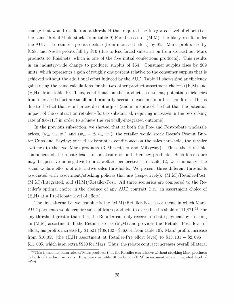
ure 4 reports the profits of each firm (ignoring the fixed cost of restocking) as a function

of the restocking policy, using the case in which the retailer stocks 3 Musketeers (Mars)

and Reese’s Peanut Butter Cups (Hershey) in the final two slots. We see that for both

Mars and the Retailer, profits are monotonically decreasing as downstream effort falls, or

the expected number of consumers between restocking visits rises. However, for Hershey

and Nestle, profits initially increase as downstream effort falls. This happens because a few

key Mars products sell-out faster than the Hershey and Nestle products, so that Hershey

and Nestle benefit from forced substitution by consumers who arrive to the machine after

the Mars products have sold out. Once effort falls below 400 expected sales, Hershey’s and

Nestle’s profits increase with downstream effort, in line with Mars and the Retailer. At these

low levels of service, downstream effort is complementary across upstream firms, so that all

upstream firms benefit from greater downstream effort. The optimal policies identified in ta-

ble 9 are always less than 270, implying that over the relevant part of the curve, downstream

effort is substitutable, and thus, increased retailer effort has a negative impact on Hershey

and Nestle. As a result, if Mars chose q to perfectly implement the vertically-integrated level

of effort, it may lead to an over-provision of effort from the industry perspective (though not

necessarily from a social perspective).

5.3 Effects of the AUD on Product Assortment

Now we consider the retailer’s endogenous choice of product assortment. We consider three

of the downstream re-stocking policies from table 9: Retailer-Pre, Retailer-Post, and Inte-

grated. We do not consider the Industry-optimal policy, because there is no credible way

to implement it with bilateral vertical arrangements. We compute profits throughout the

supply chain for each of the three re-stocking policies using the five product assortments in

table 9. In table 10, we report a subset of the most relevant product assortment choices.46

The profit numbers reported in table 10 represent the long-run expected profit from a single

machine in Group D (our ‘above-average’ group).

Our goal is to understand the relationship between the contractual structure and the

46Specifically, we report results for three of the five assortments for which payoffs are not dominated.For example, the choice of the two Nestle products (Butterfinger and Nestle Crunch) in the final two slotsis always dominated by the two better-selling Hershey products for any set of the five initial confectionsproducts.

23

retailer’s likely choice of product assortment.47 We find that at the observed wholesale

prices (wm, wh, wn), and ignoring the rebate, the retailer would choose to stock two Hershey

products in the final two slots: Reese’s Peanut Butter Cup and Payday, which we refer to

as the (H,H) assortment. This is illustrated by comparing across the three “Retailer-Pre”

rows to choose the assortment that maximizes profits in the “Retail No Rebate” column.

This outcome is obtained because the retail margin is higher on Hershey products (i.e., retail

prices are the same for both products, but wh < wm), and despite the fact that the Hershey

products achieve slightly lower sales than the Mars products.48 If we assume prices are fixed

at the post-rebate levels for all product assortments (wm−∆, wh, wn), then the retailer would

earn $36, 090 + $2, 091 = $38, 181 for stocking the two Mars products (M,M) (Milkyway and

Three Musketeeers), but $36, 661 + $1, 609 = $38, 270 for stocking (H,H). Thus, without the

threshold aspect of the rebate, the retailer would continue to stock both Hershey products.

However, if Mars were able to set the threshold so that the rebate was only paid if Mars made

more than $11,871 in revenue, then the retailer would prefer to stock both Mars products

(M,M), collect the rebate, and earn $38,181 instead of the $36,661 he would earn stocking

both Hershey products (H,H) and not collecting the rebate (i.e., the rebate provides a $1,520

increase in Retailer profit).49

5.4 Efficiency vs. Foreclosure

In this subsection we compare the efficiency and foreclosure aspects of the AUD. We define

efficiency effects as the mitigation of downstream moral hazard and inducement of additional

downstream effort. Mars can do no better than to induce the vertically-integrated level of

downstream effort.50 To quantify the efficiency effect, we hold assortment fixed, and measure

the welfare impact of moving from the “Retailer-Pre” row to the “Integrated” row in table

10. These are likely to represent upper bounds on the potential efficiency effect because we

are implicitly assuming no marginal cost of production upstream.51

We report these efficiency calculations in table 11. The first row reports the policy

47Recall, our solution concept is subgame perfection; conditional on a contract, the retailer alone choosesthe assortment and effort level.

48This is confirmed by examining the columns that report total Industry profits and consumer surplus,which are higher for both the Three Musketeers - Milkyway, or (M,M) and (H,M) assortments.

49We can work directly with Mars revenue rather than q because the wholesale prices are uniform andwe have assumed zero marginal cost of production. One also needs to confirm that offering the rebate isindividually rational for Mars. It is, as we describe in the next subsection.

50As long as effort acts as a substitute upstream, Mars’ profits rise more quickly than the cost of therebate.

51We use the calibrated $10 cost per restocking visit for the retailer.

24

change that would result from a threshold that required the Integrated level of effort (i.e.,

the same ‘Retail Understock’ from table 9).For the case of (M,M), the likely result under

the AUD, the retailer’s profits decline (from increased effort) by $55, Mars’ profits rise by

$128, and Nestle profits fall by $10 (due to less forced substitution from stocked-out Mars

products to Raisinets, which is one of the five initial confections products). This results

in an industry-wide change to producer surplus of $64. Consumer surplus rises by 209

units, which represents a gain of roughly one percent relative to the consumer surplus that is

achieved without the additional effort induced by the AUD. Table 11 shows similar efficiency

gains using the same calculations for the two other product assortment choices ((H,M) and

(H,H)) from table 10. Thus, conditional on the product assortment, potential efficiencies

from increased effort are small, and primarily accrue to consumers rather than firms. This is

due to the fact that retail prices do not adjust (and is in spite of the fact that the potential

impact of the contract on retailer effort is substantial, requiring increases in the re-stocking

rate of 8.6-11% in order to achieve the vertically-integrated outcome).

In the previous subsection, we showed that at both the Pre- and Post-rebate wholesale

prices, (wm, wh, wn) and (wm − ∆, wh, wn), the retailer would stock Reese’s Peanut But-

ter Cups and Payday; once the discount is conditioned on the sales threshold, the retailer

switches to the two Mars products (3 Musketeers and Milkyway). Thus, the threshold

component of the rebate leads to foreclosure of both Hershey products. Such foreclosure

may be positive or negative from a welfare perspective. In table 12, we summarize the

social welfare effects of alternative sales thresholds. We present three different thresholds

associated with assortment/stocking policies that are (respectively): (M,M)/Retailer-Post,

(M,M)/Integrated, and (H,M)/Retailer-Post. All three scenarios are compared to the Re-

tailer’s optimal choice in the absence of any AUD contract (i.e., an assortment choice of

(H,H) at a Pre-Rebate level of effort).

The first alternative we examine is the (M,M)/Retailer-Post assortment, in which Mars’

AUD payments would require sales of Mars products to exceed a threshold of 11,871.52 For

any threshold greater than this, the Retailer can only receive a rebate payment by stocking

an (M,M) assortment. If the Retailer stocks (M,M) and provides the ‘Retailer-Post’ level of

effort, his profits increase by $1,521 ($38,182 - $36,661 from table 10). Mars’ profits increase

from $10,055 (the (H,H) assortment at Retailer-Pre effort level) to $13, 101 − $2, 096 =

$11, 005, which is an extra $950 for Mars. Thus, the rebate contract increases overall bilateral

52This is the maximum sales of Mars products that the Retailer can achieve without stocking Mars productsin both of the last two slots. It appears in table 10 under an (H,M) assortment at an integrated level ofeffort.

25

surplus by $2,471 ($1,521 for the retailer and $950 for Mars). However, because Hershey’s

loss exceeds the Retailer’s gain, Hershey could avoid exclusion by lowering its wholesale price

to cw = 12.83 cents per unit from its current level of around 40 cents (thus transferring $1,521

to the Retailer). We do not have hard evidence on manufacturing costs in the industry, but

we believe them to be in the neighborhood of 15-20 cents per bar. If so, Hershey would not

be able to avoid exclusion once manufacturing costs were taken into account. The net gain

in the bilateral profits of the Retailer and Mars of $2,471 exceeds Hershey’s profits of $2,173,

and so the rebate appears to increase overall profit for the industry by $298, and consumer

surplus is higher.

The second alternative sets a higher threshold (equal to 13,195) in order to induce the

higher, vertically-integrated level of Retailer effort. At this higher threshold, the Retailer’s

profit increases by $1,485 relative to the non-rebating (H,H) option, and Mars’ profits in-

crease by $1,029. Hershey still loses $2,173, implying that they could avoid exclusion with

a wholesale price of 13.54 cents per unit. Overall industry profits again exceed those under

the (H,H)/Retailer-Pre outcome, by $302 for the industry, and consumer surplus increases

by 444 units.

The Chicago Critique predicts that exclusion should only occur if it maximizes overall

industry profits (Mars + Retailer + Hershey + Nestle), otherwise Hershey and/or Nestle

will act to prevent exclusion (by setting p = mc). In spite of the net increases in social

surplus induced by the AUD, this does not appear to hold, as the AUD leads to a product

assortment that does not maximize industry profits. The assortment that is optimal for the

industry and society allows for one Hershey’s product (Reese’s Peanut Butter Cup) and one

Mars product (Three Musketeers), which we label (H,M). The final column in table 12 shows

that at a Post-Rebate level of effort, this assortment leads to higher consumer and industry

surplus than even the vertically-integrated firm can attain with (M,M).53

Finally, a separate question is whether Mars could use an alternative AUD contract to

implement (H,M), and whether they might want to. Returning to the third column of table

12, one can imagine reducing the threshold so that the rebate was paid as long as the retailer

stocked no more than one Hershey product (i.e., Mars’ threshold would exceed 10,251). In

this case, Mars would actually be -$174 worse off than it would be by not offering a rebate

and having the retailer choose (H,H). Unless it can obtain exclusivity, the current rebate is

essentially too costly for Mars. Another approach might be to reduce the generosity of the

53A threshold exceeding 10,251 is required to rule out the possibility that the retailer chooses an (H,H)assortment with a high (vertically-integrated) level of effort.

26

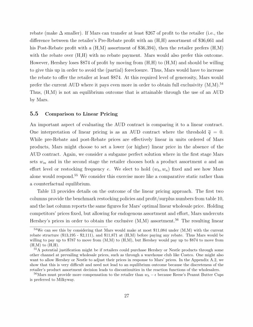
rebate (make ∆ smaller). If Mars can transfer at least $267 of profit to the retailer (i.e., the

difference between the retailer’s Pre-Rebate profit with an (H,H) assortment of $36,661 and

his Post-Rebate profit with a (H,M) assortment of $36,394), then the retailer prefers (H,M)

with the rebate over (H,H) with no rebate payment. Mars would also prefer this outcome.

However, Hershey loses $874 of profit by moving from (H,H) to (H,M) and should be willing

to give this up in order to avoid the (partial) foreclosure. Thus, Mars would have to increase

the rebate to offer the retailer at least $874. At this required level of generosity, Mars would

prefer the current AUD where it pays even more in order to obtain full exclusivity (M,M).54

Thus, (H,M) is not an equilibrium outcome that is attainable through the use of an AUD

by Mars.

5.5 Comparison to Linear Pricing

An important aspect of evaluating the AUD contract is comparing it to a linear contract.

One interpretation of linear pricing is as an AUD contract where the threshold q = 0.

While pre-Rebate and post-Rebate prices are effectively linear in units ordered of Mars

products, Mars might choose to set a lower (or higher) linear price in the absence of the

AUD contract. Again, we consider a subgame perfect solution where in the first stage Mars

sets wm and in the second stage the retailer chooses both a product assortment a and an

effort level or restocking frequency e. We elect to hold (wh, wn) fixed and see how Mars

alone would respond.55 We consider this exercise more like a comparative static rather than

a counterfactual equilibrium.

Table 13 provides details on the outcome of the linear pricing approach. The first two

columns provide the benchmark restocking policies and profit/surplus numbers from table 10,

and the last column reports the same figures for Mars’ optimal linear wholesale price. Holding

competitors’ prices fixed, but allowing for endogenous assortment and effort, Mars undercuts

Hershey’s prices in order to obtain the exclusive (M,M) assortment.56 The resulting linear

54We can see this by considering that Mars would make at most $11,084 under (M,M) with the currentrebate structure ($13,195 - $2,111), and $11,871 at (H,M) before paying any rebate. Thus Mars would bewilling to pay up to $787 to move from (M,M) to (H,M), but Hershey would pay up to $874 to move from(H,M) to (H,H).

55A potential justification might be if retailers could purchase Hershey or Nestle products through someother channel at prevailing wholesale prices, such as through a warehouse club like Costco. One might alsowant to allow Hershey or Nestle to adjust their prices in response to Mars’ prices. In the Appendix A.2, weshow that this is very difficult and need not lead to an equilibrium outcome because the discreteness of theretailer’s product assortment decision leads to discontinuities in the reaction functions of the wholesalers.

56Mars must provide more compensation to the retailer than wh − ε because Reese’s Peanut Butter Cupsis preferred to Milkyway.

27

price of 41.36 cents per unit is more than 15% lower than the observed post-rebate price. This

lower price induces greater retail effort than the post-Rebate prices (ignoring the threshold),

resulting in a retailer restocking policy of waiting for 257 consumers instead of 259. However,

the lower linear price does not not reach the vertically-integrated optimal rate of restocking

after 243 consumers. We hold retail prices fixed, so consumer surplus is affected only by

the assortment and effort level, and not the wholesale prices directly. Thus, consumers are

slightly better off with the effort and assortment decisions that arise under linear wholesale

pricing than they are under the post-rebate wholesale pricing, but not as well off as they

are under the vertically-integrated rebate outcome (which can be attained with the optimal

choice of q under the AUD). From the social surplus perspective, the costs of banning the

AUD and restricting Mars to linear contracts appear to be small, especially if it is difficult

to choose an appropriate threshold q. For example, if Mars set the sales threshold too low,

the linear contract outperforms the AUD contract. However, consistent with some of the

existing literature (see Kolay, Shaffer, and Ordover (2004)) the AUD has the potential to

shift substantial rents from retailers to upstream firms (in this case, almost 10% of Mars’

revenue).

5.6 Implications for Mergers

Vending is one of many industries for which retail prices are often fixed across similar prod-

ucts and under different vertical arrangements.57 Indeed, there are many industries for which

the primary strategic variable is not retail price, but rather a slotting fee or other transfer

payment between vertically-separated firms. Thus, our ability to evaluate the impact of a

potential upstream merger may turn on how the merger affects payments between firms in

the vertical channel.

In this analysis, we consider the impact of three potential mergers (Mars-Hershey, Mars-

Nestle, and Hershey-Nestle) on the AUD terms offered to the retailer by Mars. Given

the degree of concentration in the confections industry, antitrust authorities would likely

investigate proposed mergers, especially mergers involving Mars.58 In order to analyze the

impact of any potential merger, we conduct the same exercise as before, but consider the

incentives of the merged firm.

Table 14 considers the impact of a Mars-Hershey merger. We assume that the Hershey

product (Reeses) is priced at the Mars wholesale price and included in Mars’ rebate contract

57For example, theatrical movie exhibition and many digital markets, such as downloads or streamingservices for music and movies, all feature fixed retail pricing across different products and contractual terms.

58For a related analysis of diversion ratios in this market, see Conlon and Mortimer (2013b).

28

after the merger. The merged (Mars-Hershey) firm is now happy for consumers to substitute

to Reese’s Peanut Butter Cups, and the AUD is able to achieve the industry-optimal (and

socially-optimal) product assortment of (H,M). The merged firm faces competition from

Nestle (Crunch and Butterfinger), which charges lower wholesale prices.59 In the absence

of an AUD, the Retailer maximizes profits by stocking the two Nestle products (earning

$36,601), but the AUD is able to induce the retailer to choose (H,M), as well as the ef-

fort level that would be set by the vertically-integrated firm (earning $38,445 = $36,340 +

$2,105). Appendix A.4 provides details and discussion on two additional mergers: Mars-

Nestle and Hershey-Nestle. A pattern similar to the results from table 10 emerges in both

cases. Specifically, the retailer’s optimal assortment in the absence of an AUD is (H,H), but

the AUD induces the retailer to stock (M,M). The (M,M) assortment attains greater indus-

try and social surplus, but does not achieve the industry- or socially-optimal assortment of

(H,M).

We summarize the impact of all three mergers for the AUD contract in Table 15. We

focus on the extent to which Mars could reduce the generosity of the rebate, holding retail

prices fixed and assuming a 15 cent marginal cost of production for all upstream firms. The

first column reports outcomes in the absence of any mergers. In this case, we find that Mars

can only reduce the rebate by 4% while continuing to foreclose Hershey from the market,

giving some indication that the AUD contract is being set close to optimally. The second

column reports outcomes after a hypothetical merger of Mars and Hershey. In this case, the

merged Mars-Hershey firm is able to implement the industry-optimal product assortment of

(H,M). Holding fixed the terms of the rebate, this merger appears to be an unambiguous

improvement for consumers, the industry, and to the merging parties. However, since Nestle

is less strong as a competitor (and because (H,M) is more profitable than (M,M)), Mars

seems likely to reduce the generosity of the rebate by 18.7% (assuming zero marginal cost)

or 42.3% (assuming a 15 cent marginal cost for the industry). If this occurred, it would

reduce retailer (post-rebate) profits by $890 (i.e., a 42.3% reduction of the retailer’s rebate

payment of $2,105).

The third column reports outcomes after a hypothetical Mars-Nestle merger. The pri-

mary effect of this merger is that Mars is able to control additional profits from Raisinets.

This means that Mars can transfer the same amount of profits to the retailer with a smaller

rebate (in percentage terms). Assuming a 15 cent marginal cost, the merged firm could

reduce the rebate by roughly 12%. Finally, the last column provides outcomes under a

59We assume Nestle’s wholesale prices do not adjust after the Mars-Hershey merger.

29

hypothetical Hershey-Nestle merger. The primary impact in this case is that the merged

firm has control of more surplus when trying to avoid exclusion. However, the profit loss is

relatively unaffected, so it appears unlikely to substantially impact the rebate paid to the

retailer.

Throughout the paper, we report the variable profits for the retailer; it is likely that

his overall operating profits are substantially lower. In the Intel case, the rebate program

was reported to account for more than one quarter of Dell’s operating profits. Based on

communication with industry participants, we think that the Mars rebate may be an even

larger fraction of operating profits in the vending industry. This means that a 42% rebate

reduction (implied by the hypothetical Mars-Hershey merger) may represent a substantial

fraction of (or even exceed) the overall operating profits of the retailer.

6 Conclusion

This paper provides the first empirical evidence regarding the potential efficiency and foreclo-

sure aspects of an AUD contract, which has been at the center of recent antitrust litigation.

In the recent Meritor v. Eaton case, the Third Circuit ruled that conditional payments from

upstream to downstream firms could be considered anti-competitive even in the absence of

below-cost pricing, and that arguments weighing efficiency and anticompetitive effects could

be presented.

In order to understand these tradeoffs, our framework incorporates both endogenous re-

tailer effort and product assortment decisions. We link these outcomes to the downstream

substitutability of products, and the distribution of effort costs throughout the supply chain.

We measure both of these quantities empirically using both a field experiment and a para-

metric demand model. We show that the AUD contracts we observe have the potential

to increase effort provision by 9-11%, but these rents are mostly captured by consumers.

The AUD also enables the dominant firm, Mars, to foreclose Hershey by leveraging profits

from dominant brands such as Snickers and Peanut M&Ms, and to obtain shelf-space for

underperforming brands such as Milkyway.

We find that at the prevailing wholesale prices, this foreclosure enhances the profitability

of the overall industry and improves social surplus, but does not lead to a product assort-

ment that maximizes industry profits. Thus, the outcome of the contract falls short of the

prediction of the Chicago Critique. We note that in the absence of the AUD contract, man-

ufacturers may charge different wholesale prices. In a limited comparison of Mars’ optimal

linear wholesale prices to the AUD contract, we find that the primary difference between the

30

AUD and linear wholesale pricing is the allocation of profits between the dominant upstream

firm and the retailer. The differential impact on social welfare is small, and depends on how

the dominant firm sets the quantity threshold in the AUD. Finally, we explore the potential

impact of an upstream merger on the likely terms of the AUD contract, holding retail prices

fixed. We find that a merger between the two largest upstream firms has the potential to

induce the socially-optimal product assortment, but may also lead to a reduction in the

rebate payments to retailers.

In addition to providing results on an All-Units Discount, our detailed data and experi-

mental variation allow us to present some of the first empirical evidence on the welfare effects

of vertical arrangements in a setting that accounts for downstream moral hazard and effort

provision.

31

References

Aghion, P., and P. Bolton (1987): “Contracts as Barriers to Entry,” American EconomicReview, 77(3), 388–401.

Asker, J. (2005): “Diagnosing Foreclosure due to Exclusive Dealing,” Working Paper.

Asker, J., and H. Bar-Isaac (2014): “Raising Retailers’ Profits: On Vertical Practicesand the Exclusion of Rivals,” American Economic Review, 104(2).

Baker, G. P., and T. N. Hubbard (2003): “Make Versus Buy in Trucking: AssetOwnership, Job Design, and Information,” American Economic Review, 93(3), 551–572.

Bernheim, B. D., and M. Whinston (1998): “Exclusive Dealing,” Journal of PoliticalEconomy, 106(1), 64–103.

Berry, S. (1994): “Estimating discrete-choice models of product differentiation,” RANDJournal of Economics, 25(2), 242–261.

Bork, R. (1978): The Antitrust Paradox. New York: Free Press.

Brickley, J., and F. Dark (1987): “The Choice of Organizational Form: The Case ofFranchising,” Journal of Financial Economics, 18, 401–420.

Chao, Y., and G. Tan (2013): “All-Units Discounts, Quantity Forcing, and CapacityConstraint,” Working Paper.

Chen, C.-W. (2014): “Estimating the Foreclosure Effect of Exclusive Dealing: Evidencefrom the Entry of Specialty Beer Producers,” Working Paper.

Chipty, T. (2001): “Vertical Inegration, Market Foreclosure, and Consumer Welfare in theCable Television Industry,” American Economic Review, 91(3), 428–53.

Conlon, C., and J. H. Mortimer (2013a): “Demand Estimation Under IncompleteProduct Availability,” American Economic Journal: Microeconomics, 5(4), 1–30.

Conlon, C. T., and J. H. Mortimer (2010): “Effects of Product Availability: Experi-mental Evidence,” NBER Working Paper No. 16506.

(2013b): “An Experimental Approach to Merger Evaluation,” NBER WorkingPaper No. 19703.

Deneckere, R., H. Marvel, and J. Peck (1996): “Demand Uncertainty Inventoriesand Resale Price Maintenance,” Quarterly Journal of Economics, 111(3), 885–914.

(1997): “Demand Uncertainty and Price Maintenance: Markdowns as DestructiveCompetition,” American Economic Review, 87(4), 619–641.

32

Figueroa, N., E. Ide, and J.-P. Montero (2014): “Discounts as a Barrier to Entry,”Working Paper.

Fumagalli, C., and M. Motta (2006): “Exclusive Dealing and Entry, when BuyersCompete,” American Economic Review, 96(3), 785–795.

Gil, R. (2007): “Make-or-buy in Movies: Integration and Ex-post Renegotiation,” Inter-national Journal of Industrial Organization, 25(4), 643–655.

Hotz, V. J., and R. A. Miller (1993): “Conditional Choice Probabilities and the Esti-mation of Dynamic Models,” Review of Economic Studies, 60(3), 497–529.

Hubbard, T. N. (1998): “An empirical examination of moral hazard in the vehicle inspec-tion market,” Rand Journal of Economics, 29(2), 406–426.

Klein, B., and K. M. Murphy (1988): “Vertical Restraints as Contract EnforcementMechanisms,” Journal of Law and Economics, 31(2), 265–297.

Kolay, S., G. Shaffer, and J. A. Ordover (2004): “All-Units Discounts in RetailContracts,” Journal of Economics and Managment Strategy, 13(3), 429–459.

Lafontaine, F. (1992): “Agency Theory and Franchising: Some Empirical Results,”RAND Journal of Economics, 23, 263–283.

Lafontaine, F., and M. Slade (2007): “Vertical Integration and Firm Boundaries: TheEvidence,” Journal of Economic Literature, 45(3), 629–685.

(2008): “Exclusive Contracts and Vertical Restraints: Empirical Evidence andPublic Policy,” in Handbook of Antitrust Economics, ed. by P. Buccirossi, pp. 391–414.MIT Press, Cambridge, MA.

Lee, R. S. (2013): “Vertical Integration and Exclusivity in Platform and Two-Sided Mar-kets,” American Economic Review, 103(7), 2960–3000.

McFadden, D. (1978): “Modelling the Choice of Residential Location,” in Spatial Inter-action Theory and Planning Models, ed. by A. Karlqvist, L. Lundsqvist, F. Snickars, and

J. Weibull. North-Holland.

O’Brien, D. P. (2013): “All-Units Discounts and Double Moral Hazard,” Working Paper.

Posner, R. (1976): Antitrust Law: An Economic Perspective. University of Chicago Press.

Rasmusen, E. B., J. M. Ramseyer, and J. Wiley, John S. (1991): “Naked Exclusion,”The American Economic Review, 81(5), pp. 1137–1145.

Rust, J. (1987): “Optimal Replacement of GMC Bus Engines: An Empirical Model ofHarold Zurcher,” Econometrica, 55(5), 999–1033.

33

Sass, T. (2005): “The competitive effects of exclusive dealing: Evidence from the U.S. beerindustry,” International Journal of Industrial Organization, 23(3-4), 203–225.

Segal, I. R., and M. D. Whinston (2000): “Naked Exclusion: Comment,” AmericanEconomic Review, 90(1), 296–309.

Shaffer, G. (1991a): “Capturing Strategic Rent: Full-Line Forcing, Brand Discounts,Aggregate Rebates, and Maximum Resale Price Maintenance,” Journal of Industrial Eco-nomics, 39(5), 557–575.

(1991b): “Slotting Allowances and Resale Price Maintenance: A Comparison ofFacilitating Practices,” RAND Journal of Economics, 22(1), 120–135.

Shepard, A. (1993): “Contractual Form, Retail Price, and Asset Characteristics in GasolineRetailing,” RAND Journal of Economics, 24(1), 58–77.

Sinkinson, M. (2014): “Pricing and Entry Incentives with Exclusive Contracts: Evidencefrom Smartphones,” Working Paper.

Stokey, N. L., R. Lucas, and E. Prescott (1989): Recursive Methods for EconomicDynamics. Harvard University Press.

Sudhir, K., and V. R. Rao (2006): “Are Slotting Allowances Efficiency-Enhancing orAnti-Competitive?,” Journal of Marketing Research, 43(2), 137–155.

Telser, L. (1960): “Why Should Manufacturers Want Fair Trade?,” Journal of Law andEconomics, 3, 86–105.

Tirole, J. (1988): The Theory of Industrial Organization. MIT Press.

Train, K. (2003): Discrete Choice Methods with Simulation. Cambridge University Press.

34

Figure 1: Conventional Quantity Discount and All-Units Discount

100 1 2 3 4 5 6 7 8 9

10

0

1

2

3

4

5

6

7

8

9

X Axis

Y Ax

is

Q

W1

W2

100 1 2 3 4 5 6 7 8 9

10

0

1

2

3

4

5

6

7

8

9

X Axis

Y Ax

is

W1

W2

No Man's Land

Q

Notes: The top panel illustrates a conventional non-linear pricing schedule, in which a retailer pays awholesale price of 1 and receives a quantity discount of 0.75 for quantities greater than 6. The bottom panelillustrates an All-Units Discount with a wholesale price of 1, a threshold equal to 6, and a discount equal to0.33.

35

Figure 2: Mars Vend Operator Rebate Program

6

The Only Candy You Need To Stock In Your Machine!

#1 SellingConfection

Item in Vending!

#2 SellingConfection Item in Vending!

#3 SellingConfection Item in Vending!

Spiral #1 Spiral #2 Spiral #3 Spiral #4 Spiral #5 Spiral #6 Spiral #7 Spiral #8

M&M's® Peanut Candies

SNICKERS® BarTw ix® Carm el Cookie Bar

3 MUSKETEERS® Bar

MILKY W AY® BarM&M's® Milk Chocolate Candies

SKITTLES® Candies Original

STARBURST® Fruit Chew s Original

#4 SellingConfection Item in Vending!

#5 SellingConfection

Item in Vending!

#6 SellingConfection

Item in Vending!

#9 SellingConfection

Item in Vending!

#11 SellingConfection

Item in Vending!

• Based on the current business environment, vend operators are looking for one supplier to cover all of their Candy needs MARS - 100% Real Chocolate! MARS - 100% Real Sales!

52 Weeks Ending 10/4/09

9

2010 Vend Operator ProgramGold Rebate Level• Continuously stock 6 Singles or King Size items

Reduction from 7 must-stock items in 2009!−SNICKERS® Bar singles or king size−M&M’S®  Peanut  Chocolate  Candies  singles  or  king  size

−M&M’S®  Candies  – any other variety (Milk Chocolate, Almond, Peanut Butter or Coconut) singles or king size

−TWIX® Cookie Bar single – any variety singles or king size−3 MUSKETEERS® Bar or MILKY WAY® Bar- any variety singles or king

size−SKITTLES® Bite Size Candies or STARBURST® Fruit Chews – any

variety singles or king size

• Index >90 versus 2009Quarterly case index of 90 versus 2009

Perform ance Rebate %

$. Per Bar (singles)

GOLD Rebate SNICKERS® and M &M 's® Peanut 3% 0.015$ Index 90 All other MARS vend item s 8% 0.040$

Item s

Notes: From ‘2010 Vend Program’ materials, dated December 21, 2009; accessed on June 18, 2014 athttp://vistar.com/KansasCity/Documents/Mars%202010%20Operatopr%20rebate%20program.pdf.

36

Figure 3: Histogram of Daily Sales for Machines in Group D

8 10 12 14 16 18 20 220

500

1000

1500

2000

2500Distribution of Daily Sales for Group D

Notes: The 28 machines in group D form the basis for our counterfactual exercises. Means and standarddeviations for all machine groups are reported in table 4.

37

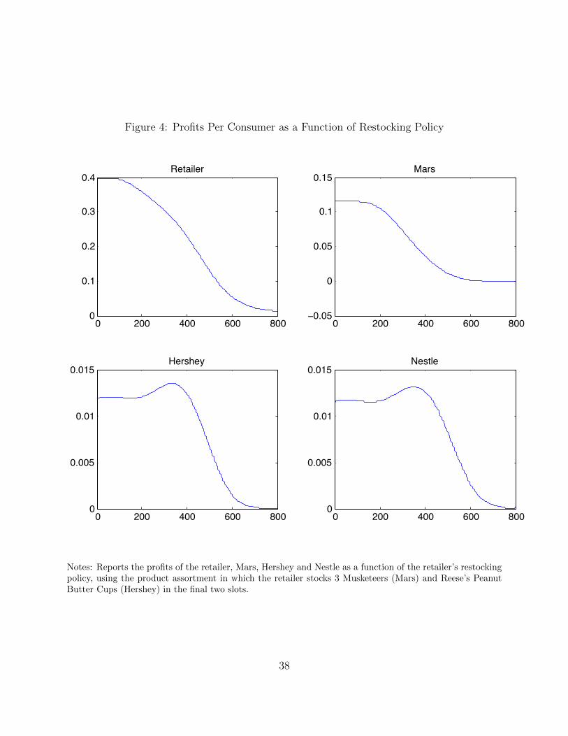
Figure 4: Profits Per Consumer as a Function of Restocking Policy

0 200 400 600 8000

0.1

0.2

0.3

0.4Retailer

0 200 400 600 800−0.05

0

0.05

0.1

0.15Mars

0 200 400 600 8000

0.005

0.01

0.015Hershey

0 200 400 600 8000

0.005

0.01

0.015Nestle

Notes: Reports the profits of the retailer, Mars, Hershey and Nestle as a function of the retailer’s restockingpolicy, using the product assortment in which the retailer stocks 3 Musketeers (Mars) and Reese’s PeanutButter Cups (Hershey) in the final two slots.

38

Table 1: Comparison of National Availability and Shares with Mark VendNational: Mark Vend:

Manu- Avail- Avail-facturer Product Rank ability Share ability Share

Mars Snickers 1 89 12.0 96 22.0Mars Peanut M&Ms 2 88 10.7 96 23.0Mars Twix Bar 3 67 7.7 79 13.0Hershey Reeses Peanut Butter Cups 4 72 5.5 29 3.7Mars Three Musketeers 5 57 4.3 34 4.3Mars Plain M&Ms 6 65 4.2 47 6.4Mars Starburst 7 38 3.9 16 1.0Mars Skittles 8 43 3.9 77 6.5Nestle Butterfinger 9 52 3.2 33 2.7Hershey Hershey with Almond 10 39 3.0 0 0Nestle Raisinets >45 N/R N/R 78 8.9

Notes: National Rank, Availability and Share refers to total US sales for the 12 weeks ending May 14, 2000,

reported by Management Science Associates, Inc., at http://www.allaboutvending.com/studies/study2.htm,

accessed on June 18, 2014. National figures not reported for Raisinets because they are outside of the 45

top-ranked products. By manufacturer, the national shares of the top 45 products (from the same source)

are: Mars 52.0%, and Hershey 20.5%. For Mark Vend, shares are: Mars 80.0%, Hershey 8.5% (calculations

by authors). Mark Vend averages 6.86 confection facings per machine.

39

Table 2: Parametric Model Estimates

Random Coefficients Nested Logit

σSalt 0.506 0.458[.006] [.010]

σSugar 0.673 0.645[.005] [.012]

σPeanut 1.263 1.640[.037] [.028]

λChocolate 0.828 0.810[.003] [.005]

λCandyNon−Choc 0.908 0.909[.007] [.009]

λCookie/Pastry 0.845 0.866[.004] [.006]

λOther 0.883 0.894[.005] [.006]

λSaltySnack 0.720 0.696[.003] [.004]

# Nonlinear Params 3 3 5 5Product FE 73 73 73 73# Fixed Effects ξt 15256 2710 15256 2710Total Parameters 15332 2786 15334 2788LL -4372750 -4411184 -4372147 -4410649Total Sales 2960315 2960315 2960315 2960315BIC 8973960 8863881 8972783 8862840AIC 8776165 8827939 8774962 8826873

Notes: The nested logit and random coefficients estimates correspond to the choice probabilities describedin section 4 and equations 4 and 5, respectively.

40

Table 3: Products Used in Counterfactual Analyses

‘Typical Machine’ Stocks:

Confections: Salty Snacks:Peanut M&Ms Rold Gold PretzelsPlain M&Ms Snyders NibblersSnickers Ruffles CheddarTwix Caramel Cheez-It OriginalRaisinets Frito

Cookie: Dorito NachoStrawberry Pop-Tarts CheetoOat ’n Honey Granola Bar SmartfoodGrandma’s Chocolate Chip Cookie Sun ChipChocolate Chip Famous Amos Lays Potato ChipsRaspberry Knotts Baked Lays

Other: Munchos Potato ChipsRitz Bits Hot Stuff JaysRuger Vanilla WaferKar Sweet & Salty MixFarley’s Mixed Fruit SnacksPlanter’s Salted PeanutsZoo Animal Cracker Austin

Notes: These products form the base set of products for the ‘typical machine’ used in the counterfactualexercises. For each counterfactual exercise, two additional products are added to the confections category,which vary with the product assortment selected for analysis.

Table 4: Summary of Sales and Revenues for Four Clusters of Machines

Group Size Vends/Visit Revenue/Visit Avg Sales/DayMean S.D. Mean S.D. Mean S.D.

A 4 39.0 26.1 28.3 18.7 5.8 1.4B 7 88.9 39.5 70.6 33.4 24.9 3.0C 27 56.9 31.5 41.5 23.2 9.2 1.4D 28 71.6 33.8 54.3 26.8 15.1 2.0

Notes: The 66 machines in our analyses are divided into four groups of machines based on the arrival rate andthe amount of revenue collected at a service visit, using a k-means clustering algorithm. Our counterfactualanalyses are based on cluster D.

41

Table 5: Results from Snickers and Peanut M&Ms Joint Experiment

Product Control Treatment Change % Change Difference T-Stat Obs

Assorted Chocolate 104.5 227.8 123.2 117.9 1.79 6.12 69Twix Caramel 213.0 313.3 100.3 47.1 1.43 5.64 70

Reese’s Peanut Butter Cups 109.0 202.2 93.3 85.6 1.23 4.30 76Assorted Pastry 287.4 374.2 86.9 30.2 1.16 3.60 75

Plain M&Ms 132.0 196.9 64.9 49.2 1.18 3.59 55Assorted Nuts 359.3 415.8 56.6 15.7 0.73 2.28 78

Assorted Cookie 314.7 359.3 44.6 14.2 0.51 1.75 88Assorted Nonchocolate Candy 263.4 301.1 37.7 14.3 0.45 1.80 83

Assorted Chips 548.2 585.6 37.4 6.8 0.43 1.35 87Raisinets 184.0 215.9 31.9 17.3 0.44 1.99 73

Choc Chip Famous Amos 227.0 241.2 14.1 6.2 0.16 0.73 89Raspberry Knotts 70.7 79.7 8.9 12.6 0.11 0.82 79

Assorted Pretzel/Popcorn 962.0 969.8 7.8 0.8 0.09 0.24 89Assorted Fruit Snack 103.6 107.7 4.1 4.0 0.06 0.31 71

Dorito Nacho 284.5 282.6 -1.9 -0.7 -0.02 -0.10 89Assorted Baked Chips 262.8 255.8 -7.0 -2.7 -0.08 -0.35 88

Assorted Cracker 114.4 93.3 -21.1 -18.5 -0.28 -1.18 75Sun Chips 198.1 174.6 -23.5 -11.9 -0.29 -1.34 80

Cheeto 349.8 325.7 -24.1 -6.9 -0.27 -1.38 89Assorted Salty Snack 711.9 678.1 -33.9 -4.8 -0.38 -1.16 89

Assorted Energy 272.1 229.0 -43.1 -15.8 -0.61 -1.90 71Zoo Animal Cracker Austin 292.1 235.0 -57.1 -19.6 -0.64 -3.18 89

Snickers 379.4 13.2 -366.2 -96.5 -4.11 -16.00 89Peanut M&Ms 425.9 9.4 -416.5 -97.8 -4.68 -18.19 89

Total 7,170.0 6887.3 -282.7 -3.9 -3.18 -12.07 89

Notes: Control weeks are defined according to the procedure described in appendix A.3.

42

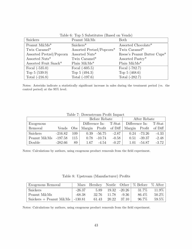
Table 6: Top 5 Substitutes (Based on Vends)Snickers Peanut M&Ms Both

Peanut M&Ms* Snickers* Assorted Chocolate*Twix Caramel* Assorted Pretzel/Popcorn* Twix Caramel*Assorted Pretzel/Popcorn Assorted Nuts* Reese’s Peanut Butter Cups*Assorted Nuts* Twix Caramel* Assorted Pastry*Assorted Fruit Snack* Plain M&Ms* Plain M&Ms*Focal (-535.0) Focal (-605.5) Focal (-782.7)Top 5 (539.9) Top 5 (494.3) Top 5 (468.6)Total (-216.8) Total (-197.6) Total (-282.7)

Notes: Asterisks indicate a statistically significant increase in sales during the treatment period (vs. thecontrol period) at the 95% level.

Table 7: Downstream Profit ImpactBefore Rebate After Rebate

Exogenous Difference In: T-Stat Difference In: T-StatRemoval Vends Obs Margin Profit of Diff Margin Profit of Diff

Snickers -216.82 109 0.39 -56.75 -2.87 0.24 -73.26 -4.33Peanut M&Ms -197.58 115 0.78 -10.74 -0.58 0.51 -39.37 -2.48Double -282.66 89 1.67 -4.54 -0.27 1.01 -54.87 -3.72

Notes: Calculations by authors, using exogenous product removals from the field experiment.

Table 8: Upstream (Manufacturer) Profits

Exogenous Removal Mars Hershey Nestle Other % Before % After

Snickers -26.37 5.89 19.32 -20.26 31.7% 11.9%Peanut M&Ms -68.38 32.76 11.78 -9.36 86.4% 50.2%Snickers + Peanut M&Ms -130.81 61.43 20.22 37.10 96.7% 59.5%

Notes: Calculations by authors, using exogenous product removals from the field experiment.

43

Table 9: Stocking Policies (Restock after how many expected sales?)

Retailer Retailer Retail RebateAdditional Products Stocked*: -Pre -Post Integrated Industry Understock Increase

Reeses PB Cup (H), 3 Musketeers (M) 267 261 244 247 9.4% 2.2%Reeses PB Cup (H), Payday (H) 263 257 237 241 11.0% 2.3%3 Musketeers (M), Milkyway (M) 264 259 243 244 8.6% 1.9%Reeses PB Cup (H), Butterfinger (N) 263 257 238 241 10.5% 2.3%Butterfinger (N), Crunch (N) 257 251 232 234 10.8% 2.3%

Notes: The five base products are: Snickers, Peanut M&Ms, Twix, Plain M&Ms (Mars), and Raisinets(Nestle). Manufacturers are denoted as (H) for Hershey’s, (N) for Nestle, and (M) for Mars. ‘Retailunderstock’ reports (Retail-Pre - Integrated)/Integrated.

Table 10: Profits under Alternate Product Assortments and Stocking Policies

Policy Retail Rebate Mars Hershey Nestle Inte- Industry Consumer(No Reb.) grated Surplus

Reeses Peanut Butter Cup (H), Three Musketeers (M)

Retailer-Pre (267) 36,399 1,875 11,719 1,302 1,260 48,117 50,679 21,685Retailer-Post (261) 36,394 1,882 11,763 1,299 1,257 48,157 50,713 21,752

Integrated (244) 36,335 1,899 11,871 1,290 1,249 48,206 50,744 21,911Reeses Peanut Butter Cup (H), Payday (H)

Retailer-Pre (263) 36,661 1,609 10,055 2,173 1,285 46,716 50,174 20,845Retailer-Post (257) 36,656 1,617 10,106 2,167 1,282 46,762 50,211 20,914

Integrated (237) 36,578 1,640 10,251 2,149 1,272 46,829 50,250 21,102Three Musketeers (M), Milkyway (M)

Retailer-Pre (264) 36,090 2,091 13,067 0 1,256 49,156 50,412 21,080Retailer-Post (259) 36,086 2,096 13,101 0 1,254 49,187 50,441 21,136Integrated (243) 36,035 2,111 13,195 0 1,246 49,230 50,476 21,289

Notes: Profit numbers represent the long-run expected profit from a single machine in Group D. Each panelrepresents one of the product assortments in table 9.

44

Table 11: Potential Efficiency Gains from Vertically-Integrated Stocking Decisions(M,M) (H,M) (H,H)

Policy Change 8.6% 9.4% 11.0%∆ Retail -55 -64 -83∆ Mars 128 196 196∆ Mars + Retailer 73 132 113∆ Hershey -12 -24∆ Nestle -10 -11 -13∆ Producer Surplus 64 65 76∆ Consumer Surplus 209 226 257%∆ Consumer Surplus 0.99% 1.04% 1.23%

Notes: Calculations based on holding assortment fixed and measuring the welfare impact of moving fromthe ‘Retailer-Pre’ row to the ‘Integrated’ row in table 10.

Table 12: Responses to Alternative Thresholds (Comparison is (H,H) Pre-Rebate)Threshold > 13,067 = 13,195 > 11,719Assortment (M,M) (M,M) (H,M)Policy Retailer-Post Integrated Retailer-Post

∆ Retail Profit 1,521 1,485 1,615∆ Mars Profit 950 1,029 -174∆ Mars+Retailer Profit 2,471 2,514 1,441∆ Hershey Profit -2,173 -2,173 -874∆ Retailer+Hershey -652 -688 741Price to Avoid Exclusion 12.83 13.54 N/A∆ Consumer Surplus 291 444 907∆ Ind 267 302 539

Notes: The social welfare effects of alternative sales thresholds compare the retailer’s ‘Pre-Rebate’ optimalstocking policy and (H,H) assortment to each of three assortment/stocking policy alternatives. Results referto the long-run impacts for a single machine in Group D. Hershey’s price is 42.75 cents per unit.

Table 13: Linear Pricing vs. AUD (Assortment is (M,M))Post-Rebate Integrated Linear Pricing

Threshold >11,871 =13,195 =0Restocking Policy 259 243 257

Retail Profit (incl’g rebate) 38,182 38,146 39,103Mars Profit 11,005 11,084 10,094

Nestle Profit 1,254 1,246 1,253Integrated (Mars-Retailer) Profit 49,187 49,230 49,197

Consumer Surplus 21,136 21,289 21,158

Notes: The optimal wholesale price under linear pricing is estimated to be 41.36 cents per unit. Hershey isexcluded in the (M,M) assortment for all three arrangements. The change in Nestle’s profits is due to theretailer’s choice of restocking policy.

45

Table 14: Profits after Mars-Hershey MergerPolicy Retail Rebate Mars/ Nestle Inte- Industry Consumer

(No Reb.) Hershey grated Surplus

Reeses Peanut Butter Cup (H), Three Musketeers (M)Retailer-Pre (267) 36,399 2,083 13,021 1,260 49,419 50,679 21,685

Retailer-Post (262) 36,395 2,089 13,055 1,257 49,451 50,708 21,741Integrated (245) 36,340 2,105 13,155 1,249 49,496 50,745 21,903

Butterfinger (N), Crunch (N)Retailer-Pre (263) 36,661 1,957 12,228 1,285 48,889 50,174 20,845Retailer-Post (257) 36,656 1,964 12,273 1,282 48,929 50,211 20,914

Integrated (240) 36,597 1,981 12,383 1,274 48,980 50,253 21,078

Notes: Profit numbers represent the long-run expected profit from a single machine in Group D. The twopanels represent the two product assortments that offer the greatest potential retailer profit under differentstocking policies and rebate payments.

Table 15: Comparison under Alternate Ownership StructuresNo Merger M-H Merger M-N Merger H-N Merger

AUD Assortment (M,M) (H,M) (M,M) (M,M)Alternative (H,H) (N,N) (H,H) (H,H)Policy Integrated Integrated Integrated Integrated∆ Retail 1,485 1,851 1,689 1,485∆ Mars 1,029 857 785 1,029∆ Bilateral 2,514 2,708 2,474 2,514∆ Competitor -2,173 -1,458 -2,173 -2,212∆ Retailer + Competitor -688 393 -484 -727∆ Consumer Surplus 444 2,473 436 444∆ Industry 302 1,251 302 302Price to Avoid Exclusion (c = 0) 13.54 n/a 9.52 14.05Rebate Reduction (c = 0) n/a 18.7% n/a n/aRebate Reduction (c = 0.15) 3.5% 42.3% 12.1% 2.3%Real Loss to Competitor (c = 0) 2,173 1,458 2,173 2,212Real Loss to Competitor (c = 0.15) 1,411 961 1,411 1,436

Notes: Table compares the welfare impacts of an exclusive Mars stocking policy under alternative ownershipstructures. This assumes threshold is set at the vertically-integrated level in order to maximize efficiencygains.

46

Appendix

A.1: Retailer Choice of Product Assortment

Even the simple problem faced by the retailer in (1) can be extremely challenging to solve.Begin by profiling out the optimal effort level conditional on e(a), so that the retailer choosesa vector a with elements aj to solve:

maxaπr(a, e(a))− c(e(a)) s.t.

∑j

aj ≤ k with aj ∈ {0, 1}

This is a binary integer programming problem, and it is quite challenging because thereare

(Jk

)possible product assortments to consider. Even in the case where π(a) − c(a) is a

linear function of the vector a, the problem reduces to the “Knapsack Problem” and is NP-hard. Once we allow for substitutes or complements in the profit function, only brute-forcesolutions exist. This means that for each possible a, we must solve a dynamic programmingproblem for retailer effort and calculate profits. For the case in which the retailer choosesseven products to stock from a set of 12, or

(127

), there are 792 possible combinations that

must be considered.60

In order to illustrate the role that an AUD plays in a retailer’s choice of product assort-ment, this section instead provides a numerical example in which an AUD contract can beused to achieve exclusion. In order to keep the example simple, we recast the retailer’s effortdecision as a capacity constraint (i.e., higher capacity is equivalent to greater retailer effort).This allows us to gain insight into the potential of an AUD contract to induce exclusionthrough the retailer’s choice of product assortment using a static model. If the efficiencygains from an AUD contract are relatively small, this intuition should mimic the results ofthe dynamic model of retailer effort.

The intuition is captured by considering two of the upstream firms, M and H, sellingto retailer R. Firm M sells two products (products 1 and 3) and offers an AUD, andFirm H sells a single product (product 2) under a simple linear price. We assume bothupstream firms face production costs of zero, and sell their products to the downstream firmat wholesale prices of (wM , wH) (i.e., M sells products 1 and 3 at the same wholesale price).We also assume that the downstream firm chooses two products to stock (i.e., [1,2], [2,3],or [1,3]), sets a single price p for all products, and faces a per-product capacity constraintr, which is equal for all products. We examine this simple setting because it captures theimportant trade-offs of the AUD contract that we observe, and also because it mimics the

60To avoid considering all possible combinations, we consider several heuristics in our empirical work. Oneuseful heuristic is the “greedy heuristic” where the retailer adds the next most profitable product in each slot.In order of profitability of Mars products, the ranking is (Peanut M&Ms, Snickers, Twix, Plain M&Ms, 3Musketeers, Milkyway, Skittles). We do not present results that consider removing Peanut M&Ms, Snickers,Twix, Plain M&Ms, or Raisinets from the choice set. In practice, we consider robustness to replacing PlainM&Ms or Raisinets, although we do not present those results because they are always strictly worse thanthe ones we do report. This implies the retailer’s decision is over only

(72

)= 21 alternatives, which is much

more manageable. We report only the best alternatives among those 21 in table 9.

47

arrangements within the chocolate confections vending market. However, it is worth notingthat many other markets may be similarly characterized.61

Consumers choose a single product from the pair of products stocked by the downstreamfirm, or the outside good (product 0). Each consumer has a preference ranking over twoof the four possible products (e.g., a consumer’s preference ranking might be [1,3], or [2,0],etc.), which determine his type. No consumer in the market ranks the outside good first. Ifa consumer’s first-choice product is not available, he chooses his second-choice product. Ifneither the first- or second-choice product is available, the consumer exits the market. Wechoose the distribution of consumer types so that demand is strongest for product 1 andweakest for product 3, and we allow for random consumer arrivals. Consumer arrivals areselected for the whole population with replacement, so demand is stochastic.62

The choice variables are: wM , and the threshold and discount terms for the AUD, q and∆, (for firm M), wH (for firm H), and a (for the downstream firm). We are interested in theconditions under which the AUD prompts the downstream firm to drop product 2 in favorof product 3 (i.e., to contract exclusively with firm M), and the welfare implications of thisdecision. We generate random arrivals of 100 consumers with replacement, setting p equalto $1, wM equal to $0.40, wH equal to $0.20, ∆ equal to $0.15, and the AUD threshold equalto 65. We assume production costs are zero, and we examine the outcome of the modelunder two different retail capacity constraints: 45 units for each product, or 65 units foreach product. We simulate the model 100,000 times to account for differences in outcomesbased on the random ordering of consumers and the stochasticity of demand.

The results of the model are shown in Table 16. Under either capacity, the rebate is paidif and only if the retailer exclusively sells M ’s products [1, 3]. Thus, even in the presence ofstochastic demand, the AUD can be used to obtain exclusivity. Under either capacity, theprofits of the retail firm and firm M are higher under the exclusive arrangement 74%(99.4%)of the time for the retailer under low(high) capacity, and 99.5%(85.4%) of the time for firmM for the low(high) capacity. The retailer prefers the exclusive arrangement less than 1% ofthe time in the absence of the AUD. Given the nature of demand and the expected profitsof R and M , both firms would have an incentive to agree to an AUD contract that led tode-facto exclusivity.

However, the two capacities yield different predictions for total (industry-level) sales. Inthe low capacity case (first column), total sales under the non-exclusive stocking arrangement[1, 2] exceed sales under the exclusive [1, 3] about 66% of the time, and are lower about 26%of the time. In the high capacity case, the results are flipped, with higher sales underthe exclusive arrangement [1, 3] about 66% of the time. We note that prices and costs arethe same across products (and the marginal cost of production is zero), so total sales areequivalent to overall industry profits. Thus, for the low-capacity case, the non-exclusivearrangement maximizes industry profits about two-thirds of the time, while in the high-capacity case the exclusive arrangement maximizes industry profits about two-thirds of the

61For example, many digital markets, such as iTunes, display limited price variation, both at the retailand wholesale levels, and do not carry all possible products.

62Random selection of consumers without replacement implies deterministic demand, although realizedsales may vary based on arrival order and capacity.

48

time. Thus, whether or not the exclusion that results from the AUD maximizes industryprofits depends on whether the impact of retail capacity on realized sales is complementaryor substitutable across upstream firms.

A.2: Solving for Endogenous Linear Prices

Allowing for endogenous linear prices (even in the absence of rebates) is a challenging exten-sion. In our setting, the retail price is fixed, and the retailer chooses a product assortment bysolving the binary integer programming problem described above. Even with three whole-sale prices that are the same across all of a manufacturer’s products (wm, wh, wn), this isa challenging problem, because the heuristic solutions employed in the previous section nolonger work.

The principle challenge is that small changes in one of the wholesale prices (e.g., wm) canresult in discrete changes in the product assortment, and discontinuous jumps in upstreamprofits. For Bertrand competition in homogeneous products, this results in the well-knownlimit pricing result. With multiple differentiated products, this implies that First-OrderConditions are not sufficient to characterize the equilibrium, and that many such equilibria(or none at all) may exist.

When we do report prices under the linear contract, we hold the prices of competitors(Hershey and Nestle) fixed and solve for the optimal Mars price wm. This parallels theexercise in Tables 9-11 under the AUD contract, though in that case we consider deviationsto check if Hershey can avoid exclusion. Even this simplified setting is challenging becauseMars’ residual profit as a function of price takes on a sawtooth form. Profits increase asprices increase, up until the retailer chooses to drop a Mars product in favor of a competitor’sproduct. There are potentially as many peaks on the sawtooth as there are dropped Marsproducts. This is demonstrated in figure 5.

We also considered a deviation in which we reduced Hershey’s price by 50% and solved forthe endogenous Mars price, though for space considerations we do not report those results inthe table. In that case, if Mars is restricted to a single linear wholesale price on all products,it is no longer worthwhile for Mars to undercut Hershey. Instead, Mars responds by setting ahigher linear wholesale price (i.e., a price between the pre- and post-rebate prices), at whichprice, the retailer selects (H,M) at a slightly lower level of effort than the post-rebate (H,M)level of 261.

A.3: Computing Treatment Effects

One goal of the product removals is to determine how product-level sales respond to changesin availability. Recall from the text that qjt denotes the sales of product j in machine-weekt, superscript 1 denotes sales when a focal product(s) is removed, superscript 0 denotes saleswhen a focal product(s) is available, the set of available products is A, and F is the setof products we remove. Thus, Q1

t =∑

j∈A\F q1jt and Q0

s =∑

j∈A q0js are the overall sales

during a treatment week, and control week respectively, and q0fs =∑

j∈F q0js is the sales of

49

the removed products. Our goal is to compute ∆qjt = q1jt − E[q0jt], the treatment effect ofremoving products(s) F on the sales of product j.

There are two challenges in implementing the removals and interpreting the data gener-ated by them. The first challenge is that there is a large amount of variation in overall salesat the weekly level independent of our exogenous removals. This can be seen in figure 6,which plots the overall sales of all machines in our sample on a weekly basis. For example, alaw firm may have a large case going to trial in a given month, and vend levels will increaseat the firm during that period. In our particular setting, many of the experiments were runduring the summer of 2007, which was a high-point in demand at these sites, most likelydue to macroeconomic conditions. In this case, using a simple measure like previous weeks’sales, or overall average sales for E[q0jt] could result in unreasonable treatment effects, suchas sales increasing due to stock-out events, or sales decreasing by more than the sales of thefocal products.

In order to deal with this challenge, we impose two simple restrictions based on consumertheory. Our first restriction is that our experimental product removals should not increaseoverall demand, so that Q0

t −Q1s ≥ 0 for treatment week t and control week s. Our second

restriction is that the product removal(s) should not reduce overall demand by more thanthe sales of the products we removed, or Q0

t −Q1s ≤ q0fs. This means we choose control weeks

s that correspond to treatment week t as follows:

{s : s 6= t, Q0t −Q1

s ∈ [0, q0fs]} (9)

While this has the nice property that it imposes the restriction on our selection of controlweeks that all products are weak substitutes, it has the disadvantage that it introduces thepotential for selection bias. The bias results from the fact that weeks with unusually highsales of the focal product q0fs are more likely to be included in our control. This bias wouldlikely overstate the costs of product removal, which would be problematic for our study.

We propose a slight modification of (9) which removes the bias. That is, we can replace

q0fs with q0fs = E[q0fs|Q0s]. An easy way to obtain the expectation is to run an OLS regression

of q0fs on Q0s, at the machine level and use the predicted value. This has the nice property

that the error is orthogonal to Q0s, which ensures that our choice of weeks is now unbiased.

The second challenge is that, although the experimental design is relatively clean, theproduct mix presented in a machine is not necessarily fixed across machines, or within amachine over long periods of time, because we rely on observational data for the controlweeks. For example, manufacturers may change their product lines, or Mark Vend maychange its stocking decisions over time. Thus, while our field experiment intends to isolatethe treatment effect of removing Snickers, we might instead compute the treatment effect ofremoving Snickers jointly with Mark Vend changing pretzel suppliers.

To mitigate this issue, we restrict our set of potential control weeks to those at the samemachine with similar product availability within the category of our experiment. In practice,two of our three treatments took place during weeks where 3 Musketeers and Reese’s PeanutButter Cups were unavailable, so we restrict our set of potential control weeks for those

50

experiments to weeks where those products were also unavailable. We denote this conditionas As ≈ At.

We use our definition of control weeks s to compute the expected control sales thatcorrespond to treatment week t as:

St = {s : s 6= t, At ≈ As, Q0t −Q1

s ∈ [0, b0 + b1Q0s]} (10)

And for each treatment week t we can compute the treatment effect as

∆qjt = q1jt −1

#St

∑s∈St

q0js (11)

While this approach has the advantage that it generates substitution patterns consistent withconsumer theory, it may be that for some treatment weeks t the set of possible control weeksSt = {∅}. Under this definition of the control, some treatment weeks constitute ‘outliers’and are excluded from the analysis. Of the 1470 machine-experiment-week combinations,991 of them have at least one corresponding control week, and at the machine-experimentlevel, 528 out of 634 have at least one corresponding control. Each included treatment weekhas an average of 24 corresponding control weeks, though this can vary considerably fromtreatment week to treatment week.63

Once we have constructed our restricted set of treatment weeks and the set of controlweeks that corresponds to each, inference is fairly straightforward. We use (11) to constructa set of pseudo-observations for the difference, and employ a paired t-test.

A.4: Additional Merger Analyses

Table 17 considers the impact of a Mars-Nestle merger. Again, we set the wholesale priceof the Nestle products to Mars’ wholesale price after the merger. Mars acquires Raisinets,which is nearly always stocked by the retailer, and which provides the merged firm withadditional profits to leverage. Substitutability between Mars’ products and Nestle’s prod-ucts (Butterfinger, Crunch, and Raisinets) is much lower than between Reeses and Mars’products, and unlike the Mars-Hershey merger, we no longer achieve the industry-optimalchoice of products in the retail market. We essentially replicate the patterns from table 10where the rebate induces the retailer to stock (M,M) instead of (H,H). Table 18 considersthe impact of the Hershey-Nestle merger, and achieves similar results. The only exception isthat the merged firm controls more brands and is a somewhat stronger competitor to Mars.

63Weeks in which the other five treatments were run (for the salty-snack and cookie categories) are excludedfrom the set of potential control weeks.

51

Table 16: Results from Varying Capacity (Numerical Example)Threshold q = 65 Capacity = 45 Capacity = 65Market:Total Sales([1,2]) > Total Sales([1,3]) 66.72% 24.16%Total Sales([1,2]) < Total Sales([1,3]) 26.49% 66.59%Total Sales([1,2]) = Total Sales([1,3]) 6.79% 9.25%Mean(Sales([1,2])-Sales([1,3])) 2.92 -2.00

as percent of sales 3.36% -2.17%Retailer:Retailer prefers [1,2] 25.80% 0.61%Retailer prefers [1,3], No Rebate 0.33% 0.69%Retailer prefers [1,3] 74.20% 99.39%Mean Retailer profit([1,2]) 60.41 63.21Mean Retailer profit([1,3]), No Rebate 50.36 56.68Mean Retailer profit([1,3]) 62.88 70.85Firm A:Firm A prefers [1,2] 0.19% 13.78%Firm A prefers [1,3] 99.55% 85.43%Mean Firm A profit under [1,2] 17.98 21.52Mean Firm A profit under [1,3] 20.96 23.62Firm A pays rebate under [1,2] 0% 0%Firm A pays rebate under [1,3] 100% 100%Firm B:Mean Firm B profits under [1,2] 8.36 7.73

Notes: Under the assumed demand patterns, retailer always stocks product 1.

52

Table 17: Profits after Mars-Nestle MergerPolicy Retail Rebate Mars/ Hershey Inte- Industry Consumer

(No Reb.) Nestle grated Surplus

Reeses Peanut Butter Cup (H), Three Musketeers (M)Retailer-Pre (267) 36,399 2,077 12,978 1,302 49,377 50,679 21,685Retailer-Post (262) 36,395 2,082 13,013 1,299 49,409 50,708 21,741

Integrated (245) 36,340 2,098 13,114 1,290 49,455 50,745 21,903Reeses Peanut Butter Cup (H), Payday (H)

Retailer-Pre (263) 36,661 1,815 11,341 2,173 48,001 50,174 20,845Retailer-Post (257) 36,656 1,822 11,388 2,167 48,045 50,211 20,914

Integrated (239) 36,591 1,842 11,511 2,151 48,102 50,253 21,086Three Musketeers (M), Milkyway (M)

Retailer-Pre (264) 36,090 2,292 14,323 0 50,412 50,412 21,080Retailer-Post (259) 36,086 2,297 14,354 0 50,441 50,441 21,136Integrated (244) 36,040 2,310 14,436 0 50,476 50,476 21,281

Notes: Profit numbers represent the long-run expected profit from a single machine in Group D. The twopanels represent the two product assortments that offer the greatest potential retailer profit under differentstocking policies and rebate payments.

Table 18: Profits after Hershey-Nestle MergerPolicy Retail Rebate Mars Hershey/ Inte- Industry Consumer

(No Reb.) Nestle grated Surplus

Reeses Peanut Butter Cup (H), Three Musketeers (M)Retailer-Pre (267) 36,399 1,875 11,719 2,562 48,117 50,679 21,685Retailer-Post (261) 36,394 1,882 11,763 2,556 48,157 50,713 21,752

Integrated (244) 36,335 1,899 11,871 2,538 48,206 50,744 21,911Reeses Peanut Butter Cup (H), Payday (H)

Retailer-Pre (263) 36,661 1,609 10,055 3,458 46,716 50,174 20,845Retailer-Post (257) 36,656 1,617 10,106 3,449 46,762 50,211 20,914

Integrated (237) 36,578 1,640 10,251 3,421 46,829 50,250 21,102Three Musketeers (M), Milkyway (M)

Retailer-Pre (264) 36,090 2,091 13,067 1,256 49,156 50,412 21,080Retailer-Post (259) 36,086 2,096 13,101 1,254 49,187 50,441 21,136Integrated (243) 36,035 2,111 13,195 1,246 49,230 50,476 21,289

Notes: Profit numbers represent the long-run expected profit from a single machine in Group D. The twopanels represent the two product assortments that offer the greatest potential retailer profit under differentstocking policies and rebate payments.

53

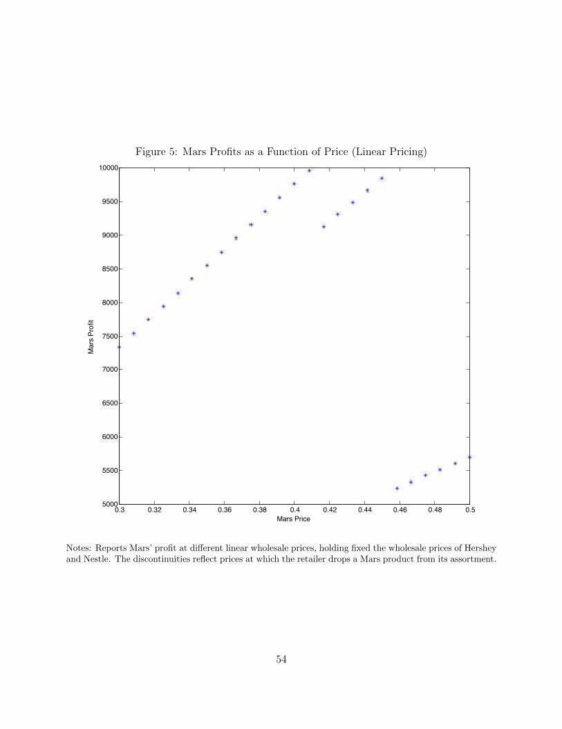
Figure 5: Mars Profits as a Function of Price (Linear Pricing)

0.3 0.32 0.34 0.36 0.38 0.4 0.42 0.44 0.46 0.48 0.55000

5500

6000

6500

7000

7500

8000

8500

9000

9500

10000

Mars Price

Mar

s Pr

ofit

Notes: Reports Mars’ profit at different linear wholesale prices, holding fixed the wholesale prices of Hersheyand Nestle. The discontinuities reflect prices at which the retailer drops a Mars product from its assortment.

54

Figure 6: Overall Weekly Sales at Site 93

600

800

1000

1200

1400

1600

0 50 100 150Week

TotalVends (mean) totalvends

Notes: Figures calculated by authors, and represent all product categories in the machines (i.e., confections,snack foods, cookies, and other).

55