IFUP-TH/2015 IFT-UAM/CSIC-15-015

Dynamically InducedPlanck Scale and Inflation

Kristjan Kannikea, Gert Hutsib, Liberato Pizzac, Antonio Racioppia,

Martti Raidala,d, Alberto Salvioe and Alessandro Strumiaa,c

a NICPB, Ravala 10, 10143 Tallinn, Estoniab Tartu Observatory, Observatooriumi 1, 61602 Toravere, Estoniac Dipartimento di Fisica dell’Universita di Pisa and INFN, Italy

d Institute of Physics, University of Tartu, Ravila 14c, 50411 Tartu, Estoniae Departamento de Fısica Teorica, Universidad Autonoma de Madrid

and Instituto de Fısica Teorica IFT-UAM/CSIC, Madrid, Spain

Abstract

Theories where the Planck scale is dynamically generated from di-

mensionless interactions provide predictive inflationary potentials and

super-Planckian field variations. We first study the minimal single

field realisation in the low-energy effective field theory limit, finding

the predictions ns ≈ 0.96 for the spectral index and r ≈ 0.13 for

the tensor-to-scalar ratio, which can be reduced down to ≈ 0.04 in

presence of large couplings. Next we consider agravity as a dimen-

sionless quantum gravity theory finding a multifield inflation that

converges towards an attractor trajectory and predicts ns ≈ 0.96

and 0.003 < r < 0.13, interpolating between the quadratic and

Starobinsky inflation. These theories relate the smallness of the weak

scale to the smallness of inflationary perturbations: both arise nat-

urally because of small couplings, implying a reheating temperature

of 107−9 GeV. A measurement of r by Keck/Bicep3 would give us

information on quantum gravity in the dimensionless scenario.

arX

iv:1

502.

0133

4v3

[as

tro-

ph.C

O]

20

May

201

5

Contents

1 Introduction 2

2 Effective field theory approach 4

2.1 Model-independent dimensionless single field inflation . . . . . . . . . . . . . . . 5

2.2 The minimal model for dimensionless single field inflation . . . . . . . . . . . . . 9

3 Inflation in agravity 13

3.1 Agravity in the Einstein frame . . . . . . . . . . . . . . . . . . . . . . . . . . . . 14

3.2 Computing multifield inflationary predictions . . . . . . . . . . . . . . . . . . . . 16

3.3 Inflationary predictions . . . . . . . . . . . . . . . . . . . . . . . . . . . . . . . . 17

4 Cosmology after inflation 19

4.1 Reheating . . . . . . . . . . . . . . . . . . . . . . . . . . . . . . . . . . . . . . . 19

4.2 Dark Matter . . . . . . . . . . . . . . . . . . . . . . . . . . . . . . . . . . . . . . 22

4.3 Inflation and the weak scale . . . . . . . . . . . . . . . . . . . . . . . . . . . . . 23

5 Conclusions 24

A RGE and the compatibility of frames 25

1 Introduction

The discovery of the Higgs boson [1, 2] and the lack (so far) of new physics challenged the

standard view on naturalness of the electroweak scale [3]. The latter led to the expectation

that the Higgs boson should be accompanied by new physics at the weak scale that is able to

provide a cut-off to quadratically divergent quantum corrections to the squared Higgs mass due

to the standard model (SM) couplings.

Given that power divergent quantum corrections do not lead to any physical effect, some

theorists are considering the possibility that the Higgs mass fine-tuning problem could be just

an unphysical artifact of the standard renormalisation procedure, that introduces an artificial

cut-off and unphysical bare parameters. On the contrary, heavy new particles coupled to the

Higgs boson would lead to large physical corrections to the Higgs mass: the associated fine-

tuning could be probed by experiments [4]. Thereby, one is led to redefine natural models as

those where new physics heavier than the weak scale is weakly coupled to the Higgs.

Starting from these phenomenological considerations, various authors tried to develop a

theoretical framework able of explaining the co-existence and the origin of the largely separated

mass scales observed in nature. Most attempts involve, in some way or another, classical scale

invariance and dynamical generation of mass scales [5, 6]. Implications for inflation have been

explored in [6, 7].

2

The largest scale observed in Nature so far is the Planck scale. Inflationary [8] generation of

primordial perturbations [9] can provide an observational window on Planck-scale physics. The

recent Bicep2/Keck/Planck common analysis [10] of the B-mode polarisation data tries to

control the astrophysical backgrounds [11] and hints at a value for the tensor-to-scalar ratio

r = 0.06 ± 0.04, in-between the previous BICEP2 [12] and Planck [13, 15] results. If future

experiments will find a statistically significant evidence for r > 0, this might be the first hint

of the quantum nature of gravity, and a precise determination of r may help us to discriminate

between different ultraviolet (UV) completions of gravity.1 This result, therefore, invites for

thorough common studies of gravity and inflation.

In this paper we explore the implications of the assumption that the Planck scale is gener-

ated dynamically, assuming that the same sector also provides inflation. The dynamics leading

to dimensional transmutation can be due to strongly-coupled or to weakly-coupled physics. We

here focus on weakly coupled dynamics, such that we can perform perturbative computations.

The literature contains studies of models with a dynamical Planck scale (see e.g. [17, 6]) and

of models with a dynamical inflaton potential (already the very first papers on inflation con-

sidered the possibility that the inflaton potential is generated dynamically by loop effects [18]

via the Coleman-Weinberg mechanism [19]). Furthermore, dynamical generation of masses is

compatible with the small observed cosmological constant provided that the scalar potential

satisfies the ‘multiple point criticality principle’ [20], that was introduced for the SM Higgs

boson and is extensively used in Higgs inflation [21, 22]. Originally, the non-minimal coupling

for the usual inflaton was considered in [23].

In this paper we combine these concepts into a consistent framework and study implications

for inflation, gravity and the electroweak scale. We follow two different approaches.

To obtain model independent results we first take an effective field theory approach and

study the minimal single field inflation from dynamical generation of the Planck scale without

knowing the theory of gravity. We assume that a complete theory of quantum gravity is

not needed either because inflation is described by Einstein gravity at sub-Planckian energy or

because some completion of Einstein gravity is weakly coupled enough. The inflaton is assumed

to be the Higgs of gravity: the pseudo-Goldstone boson of scale invariance that acquires a

vacuum expectation value (VEV) generating the Planck mass. The assumption of classical

scale invariance allows us to deal with trans-Planckian inflaton field values [24].

We find that in the limit when gravity effects can be ignored the inflationary observables

converge towards the predictions of a quadratic inflationary potential [25], up to deviations

due to higher order corrections, ns ≈ 0.96 and r ≈ 0.13+0.01−0.03. We formulate conditions when

this approximation is valid (details are collected in appendix A) and discuss the equivalence

of Einstein and Jordan frames in this limit. For large values of the non-minimal coupling to

gravity, we obtain much wider range for tensor-to-scalar ratio, r > 0.04, while the prediction

1However, an observable value of r can also be obtained for sub-Planckian field variations in certain cases

[16].

3

for scalar spectral index remains the same. This is new and much more constraining result

compared to the corresponding result in the previous scale-invariant inflation study [7] due

to extra constraints arising from the dynamically generated Planck scale and the dynamically

realised multiple point criticality principle. We present the minimal model for this scenario and

study its properties.

After the effective field theory study, we focus on a specific possibility for quantum gravity:

agravity [6], which is the dimensionless renormalizable extension of Einstein gravity. New

gravitational degrees of freedom, predicted by the theory, can be light enough to take part

in inflationary dynamics. We thereby have multifield inflation, and we find the prediction

ns ≈ 0.96 and a tensor-to-scalar ratio 0.003 < r < 0.13 that interpolates between the values

characteristic to quadratic [25] and to Starobinsky [26] inflation. In this context the smallness

of the electroweak scale is connected to the smallness of the inflationary perturbations: both

arise because the underlying theory is very weakly coupled.

In both cases, gravitational decays of the inflaton reheat the SM particles up to a temper-

ature 107 − 109 GeV.

The organization of the paper is the following. In section 2 we present our results of the

effective field theory approach to dynamically induced gravity and inflation. In section 3 we

focus on agravity and compute inflationary parameters in this quantum gravity theory. In

section 4 we collect our results on reheating and on dark matter (DM) abundance of the

universe. We conclude in section 5 and present technical details in Appendix A.

2 Effective field theory approach

In this section we present a general, model independent study of scale-invariant single field

inflation in which the Planck scale is dynamically generated by the inflaton. The main aim

of our effective field theory approach is to derive results that are valid for all possible UV

completions of gravity. We, therefore, restrict our physical parameters such that inflation occurs

within the low-energy (sub-Planckian) limit of gravity. More broadly, the hope of deriving

general implications for inflation rests on the possibility that, if the scale symmetry is broken

dynamically by a VEV induced by weakly coupled dynamics, it leaves a light scalar, which is the

pseudo-Goldstone boson of scale invariance. Two experimental facts support this assumption,

suggesting two possibilities where an effective field theory could be adequate:

1) First, the amplitude of primordial scalar perturbations is observed to be small, PR =

(2.14 ± 0.05) × 10−9 [15]. This suggests that inflation occurs at a sub-Planckian energy

E, where the gravitational coupling g(E) ∼ E/MPl (MPl = 2.4×1018 GeV is the reduced

Planck mass) is still small enough that no knowledge of the UV structure of quantum

gravity is needed. We check that our effective field theory is valid in the parameter space

we consider and that the results of our computations are trustable. We will explicitly

4

demonstrate that the results obtained in the Jordan and Einstein frames are physically

equivalent.

2) Second, the smallness of Higgs boson mass, Mh/MPl ∼ 10−16 suggests that quantum

gravity should be weakly coupled [6, 27], such that the quantum corrections to Mh are

naturally small. Soft-gravity is the idea that the growth of the gravitational coupling g(E)

with energy could be stopped by new gravitational physics at an energy E ∼ Mg low

enough that g(E) saturates at a small enough value g(E)<∼ g(Mg). Then soft-gravity can

be neglected during inflation even when Einstein gravity would become non-perturbative,

extending the domain of validity of our computations.

In practice, both possibilities above amount to ignoring quantum gravity in a controllable way.

2.1 Model-independent dimensionless single field inflation

Assuming no explicit mass scale in the fundamental Lagrangian,2 the inflaton field s, singlet

under the SM gauge group, has a scalar potential consisting only of a quartic term

V =1

4λS(s)s4, (1)

where the self-coupling λS(s) runs due to interactions (to be specified in the next subsection).

The inflaton has a non-minimal coupling to gravity −f(s)R/2, where R is the Ricci scalar,

parameterised by the dimensionless coupling ξS as

f(s) = ξSs2. (2)

We neglect the running of ξS in the limit of weak coupling of gravity in the Einstein frame

(see Appendix A for more details). We assume that the SM degrees of freedom are very

weakly coupled to the inflaton and do not affect its dynamics. For example we assume that the

allowed inflaton-Higgs mixing term s2|H|2 is negligibly small. We will show in section 4 that

this assumption is compatible with an acceptable reheating of the universe after inflation.

The coupling in eq. (2) has the same form as the usual gravitational coupling −M2PlR/2 in

the Einstein-Hilbert Lagrangian. With the assumptions made above we expect that the Planck

scale and the cosmological constant must be generated by quantum corrections encoded in the

dynamics of λS(s). This is, indeed, possible since the running of λS allows the scalar potential

of s to have a minimum at a non-zero field value. To generate the Planck scale, the VEV vs of

the inflaton field must be given by

v2s =

M2Pl

ξS. (3)

2In the full theory Lagrangian, the Higgs mass is generated via dimensional transmutation as well. We do

not discuss this topic in detail here because it depends on the exact model realisation, which is outside the

scope of this section. For further details in the agravity realisation, we refer the reader to the following sections

and to [6], where the Higgs mass was generated in such a way.

5

To compute inflationary observables we go from the Jordan frame possessing the non-minimal

coupling (2) to the Einstein frame possessing the canonical Einstein-Hilbert action of gravity

with the Weyl transformation

gEµν = Ω(s)2gµν , where Ω(s)2 =f(s)

M2Pl

=s2

v2s

. (4)

The Einstein frame scalar potential is then given by

VE(s) =V (s)

Ω(s)4=

1

4λS(s)

M4Pl

ξ2S

. (5)

At the minimum the value of this potential must be (very close to) zero in order to yield the

tiny positive vacuum energy density that gives the universe its current accelerated expansion.3

In our framework this requirement implies λS(vs) = 0. The minimum condition on λS is

dλSdt

(vs) = βλS(vs) = 0, (6)

where t = ln µ, µ is the renormalisation scale and βλS is the β function of λS. As usual, we

resum log-enhanced quantum corrections by identifying the renormalisation scale µ with the

inflaton field value s. Moreover, in order to ensure that λS(vs) = 0 is not just a stationary

point but a minimum, we need to impose the requirement β′λS(vs) ≡ d2λS(vs)/dt2 > 0. In

explicit model realisations of this scenario these requirements imply conditions on the model

parameters. We can Taylor expand λS around the minimum vs obtaining

λS(s) =1

2!β′λS(vs) ln2 s

vs+

1

3!β′′λS(vs) ln3 s

vs+ · · · , (7)

where we have used λS(vs) = βλS(vs) = 0. In any model, this is a perturbative expansion

that holds for small enough couplings.4 Assuming weak couplings in order to get the correct

small amplitude of primordial fluctuations, we will treat β′λS(vs) and β′′λS(vs) as small constant

parameters. We will show in the next subsection that this approximation can indeed hold in

the explicit model realisation.

It is convenient to rewrite VE in terms of the canonically normalised field sE in the Einstein

frame,

sE =

√1 + 6ξSξS

MPl lns

vs, (8)

3Notice that the ‘multiple point criticality’ principle of [20] arises in the context of dynamical generation of

scales because the dimensionless potential of eq. (1) necessarily has another, unphysical, minimum with zero

cosmological constant at s = 0.4Ref. [6] used a simpler approximation, neglecting also the ln3 s term. Here we investigate its impact. Of

course, an extra ln4 s term is needed in order to stabilise the potential for s vs.

6

or equivalently

s = vse

√ξS

1+6ξS

sEMPl . (9)

Inserting (7) and (9) into (5) we get

VE(sE) 'β′λS(vs)M

2Pl

8ξS (1 + 6ξS)

(1 +

√ξS

1 + 6ξS

β′′λS(vs)

3MPlβ′λS(vs)sE

)s2E, (10)

which is nothing but a quadratic potential with a cubic correction. Such a potential is symmetric

under the transformation sE → −sE and β′′λS(vs)→ −β′′λS(vs), therefore by redefining the sign

of sE we can always assume that β′′λS(vs) ≥ 0. This potential allows for two different types of

inflation:

− Negative-field inflation, when sE rolls down from negative values to zero. This corre-

sponds, in the Jordan frame, to small-field inflation (s rolls down from a value s < vs to

vs) for β′′λS(vs) > 0 and to large-field inflation (s rolls down from a value s > vs to vs) if

β′′λS(vs) < 0.

+ Positive-field inflation, when sE rolls down from positive field values to zero. This cor-

responds, in the Jordan frame, to large-field inflation for β′′λS(vs) > 0 and to small-field

inflation if β′′λS(vs) < 0.

We present in fig. 1 an example plot of the Einstein frame potential VE(sE), as computed

in the minimal model presented later in section 2.2: the potential is well approximated by the

cubic potential of eq. (10), with the following values of its parameters: ξS(vs) = 300, β′λS(vs) =

6 × 10−5 and β′′λS(vs) = 9 × 10−6. Fig. 1 also shows the potential in quadratic approximation

(dashed parabola), which is not quite perfect. We denote the field values corresponding to 60 e-

folds (s∗E) and to the end of inflation (sEend) with blue dots for negative-field inflation and with

red dots for positive-field inflation. We follow the same colour code throughout this section.

Because of the loop-induced cubic term in sE, the two inflation regimes are physically different

and can be distinguished from each other experimentally. The potential in fig. 1 yields r = 0.11

for negative-field and r = 0.16 for positive-field inflation. For large ξS, β′λS(vs) and β′′λS(vs)

(given by large couplings), higher order terms in the expansion (7) will become important. The

cubic approximation breaks down and one has to consider numerically exact running of the

couplings.

Under the soft-gravity assumption (described as point 2 at the beginning of section 2), this

computation holds in all its parameter space. The model-independent approach (described as

point 1) holds instead only as long as Einstein gravity can be neglected. It is simple to check

the validity range of the computations in the Einstein frame. The condition is

(VE(sE))1/4 MPl, (11)

7

- - /

×-

×-

×-

×-()/

*

*

Figure 1: The Einstein-frame inflation potential VE(sE) (solid) as computed in the minimal

model of section 2.2, and its quadratic approximation (dashed). Blue dots show s∗E and sEend

for negative-field inflation and red dots for positive-field inflation. Other parameters are specified

in the text.

so that we can consistently ignore quantum gravity corrections. Such a condition should be

realised at least for sE = s∗E, which corresponds to the maximum potential value for the inflation

computations. Ignoring the cubic correction in eq. (10) we get

1

8

β′λS(vs)

ξS(6ξS + 1)(MPl

s∗E

)2

. (12)

We considered values of β′λS(vs), β′′λS

(vs) and ξS so that eq. (11) is satisfied, so that our compu-

tations are consistent and we can safely ignore quantum gravity corrections. The consistency

condition (11) can also be expressed in the Jordan frame as

(VJ(s))1/4 √ξS|s|, (13)

leading to the same result expressed in (12) after taking into account the relation between s

and sE (see eq. (8)).

To better understand how the predictions of negative-field inflation differ from positive-

field inflation due to the presence of the cubic term β′′λS(vs)/β′λS

(vs), we expand the slow-roll

parameters at first order in it. The scalar spectral index ns and the tensor-to-scalar ratio r are

given by

r ' 8

N∓ 32

√2

9

√ξS

6ξS + 1

β′′λS(vs)

β′λS(vs)

(1√2N− 1

4N2

),

ns ' 1− r

4±

√ξS

6ξS + 1

β′′λS(vs)

β′λS(vs)

√r

3√

2,

(14)

8

where N denotes the number of e-folds, and the signs +(−) should be used for the positive-field

inflation and −(+) for negative-field inflation. We see that (14) predicts somewhat different

behaviour of ns and r for the positive-field and negative-field inflation scenarios.

The approximation (14) breaks down if ξS and other couplings are large. In that case the

deviation of r from quadratic inflation can be large too, as seen in the minimal model realisation

presented in subsection 2.2.

In conclusion, the observed small value of PR favours a small inflaton self-coupling. If other

couplings are small as well, then the Einstein-frame inflaton potential is well approximated by

a quadratic potential. If other couplings are large, the deviation of r from quadratic inflation

can be strong, as shown in fig. 3. In section 3 we will show that in agravity [6] — a concrete UV

completion of gravity — dimensionless inflation can give a significantly smaller value of r if all

couplings are small. Basically this will arise because agravity realises the soft-gravity scenario

by adding to the Lagrangian dimensionless terms of R2 form (as in Starobinsky inflation),

leading to extra light scalars.

2.2 The minimal model for dimensionless single field inflation

In this subsection we present the minimal model that dynamically reproduces all features of

dimensionless single field inflation considered in the previous subsection. Besides the inflaton

s, the minimal model contains another real scalar σ and a Majorana fermion ψ. This is the

minimal field content that is needed to achieve condition (6) dynamically. Indeed, the portal

coupling of the inflaton with the extra scalar is needed to trigger dimensional transmutation

while the extra fermion is needed to be able to tune the minimum of the potential according

to the multiple point criticality principle. The latter is possible since the scalar and fermion

couplings contribute to the running of the inflaton self-coupling with opposite signs, as is

apparent from the RGEs presented in appendix A. This fact has also been used to achieve the

multiple point criticality in Higgs inflation [28].

Thus the Jordan frame Lagrangian of the minimal model is√−gJL J =

√−gJ

[LSM −

ξS2s2R +

(∂s)2

2+

(∂σ)2

2+i

2ψc /Dψ + LY − V

], (15)

LY =1

2ySsψ

cψ +1

2yσσψ

cψ, (16)

V =1

4λSs

4 +1

4λSσs

2σ2 +1

4λσσ

4, (17)

where we neglected the couplings to the SM fields, as suggested by the hierarchy problem. In

the Einstein frame, the Lagrangian reads√−gEL E =

√−gE

[LSM

Ω(s)4− 1

2M2

PlR +(∂sE)2

2+

(∂σE)2

2+i

2ψcE /DψE + LYE − VE + · · ·

],

(18)

9

LYE =1

2ySvsψ

cEψE +

1

2yσσEψ

cEψE ≡

1

2mψψ

cEψE +

1

2yσσEψ

cEψE, (19)

VE =1

4λSv

4s +

1

4λSσv

2sσ

2E +

1

4λσσ

4E ≡ Λ +

1

2m2σσ

2E +

1

4λσσ

4E, (20)

where, in order to have canonical kinetic terms, the Einstein-frame scalar and fermion fields

are defined as

σE =σ

Ω(s), ψE =

ψ

Ω(s)32

, (21)

whereas gauge vectors are invariant under the transformation. It can be shown that the deriva-

tive of the denominator in (21) cancels out in the fermion kinetic term because of the spin

connection contribution in /D [29, 30, 31], whereas for scalars (with the exception of the canon-

ically normalised inflaton field sE) it induces a derivative interaction. For simplicity we omit

these details in the above Lagrangian, which are essential for reheating the universe after infla-

tion and will be discussed in section 4. Below, we work in the Einstein frame and omit indices

(except for sE).

Note that in the scalar potential and in the Yukawa terms of the high scale inflationary

physics the scale transformation is equivalent to the substitution s→ vs and, therefore, in the

Einstein frame the fermion ψ and the scalar σ do not have couplings to the inflaton at tree-level.

The Jordan frame self-coupling term of the inflaton becomes the cosmological constant Λ in

the Einstein frame potential (20) (equivalent to (5)). The Yukawa and quartic portal terms of

the inflaton become mass terms, giving the mass of the σ field in the Einstein frame by

m2σ =

1

2λSσ(vs)

M2Pl

ξS, (22)

and the mass of the fermion ψ in the Einstein frame by

mψ = yS(vs)MPl√ξS. (23)

The scalar potential depends on the inflaton field only due to the running of the scalar

couplings.

The renormalisation group equations (RGEs) of the model in the weakly coupled gravity

limit are computed in appendix A. In the Jordan frame, gravity does not contribute to the

running of the couplings at the one-loop level [48]. The transformation to the Einstein frame

mixes the gravitational and scalar degrees of freedom such that in the Einstein frame the matter

RGEs get contributions from gravity, that we neglect. We can explicitly verify the equivalence

of the frames only up to these neglected effects, as discussed in appendix A around eq. (76).

We suppose that inflation takes place along the s field direction (that is, σ = 0). We will see

later that such an assumption is self-consistent: since the scalar σ will turn out to be heavier

than the inflaton, it does not take part in inflation. As discussed earlier, we need to realise

λS(vs) = βλS(vs) = 0. Imposing λS(vs) = 0, the second condition becomes (see eq. (62)),

16π2βλS(vs) =1

2λ2Sσ − 4y4

S = 0, (24)

10

- - ×

×

×

×

×

ξ

/

- - -

-

-

ξ

λσ

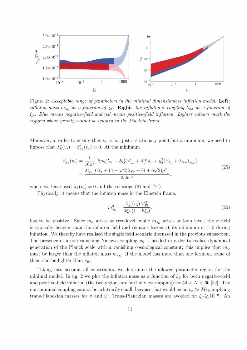
Figure 2: Acceptable range of parameters in the minimal dimensionless inflation model. Left:

inflaton mass msE as a function of ξS. Right: the inflaton-σ coupling λSσ as a function of

ξS. Blue means negative-field and red means positive-field inflation. Lighter colours mark the

regions where gravity cannot be ignored in the Einstein frame.

Moreover, in order to ensure that vs is not just a stationary point but a minimum, we need to

impose that λ′′S(vs) = β′λS(vs) > 0. At the minimum

β′λS(vs) =1

16π2

[8yS(λS − 2y2

S)βyS + 4(9λS + y2S)βλS + λSσβλSσ

]=λ2Sσ

[6λσ + (4−

√2)λSσ − (4 + 6

√2)y2

σ

]256π4

,

(25)

where we have used λS(vs) = 0 and the relations (3) and (24).

Physically, it means that the inflaton mass in the Einstein frame,

m2sE

=β′λs(vs)M

2Pl

4ξS (1 + 6ξs), (26)

has to be positive. Since mσ arises at tree-level, while msE arises at loop level, the σ field

is typically heavier than the inflaton field and remains frozen at its minimum σ = 0 during

inflation. We thereby have realised the single field scenario discussed in the previous subsection.

The presence of a non-vanishing Yukawa coupling yS is needed in order to realise dynamical

generation of the Planck scale with a vanishing cosmological constant; this implies that mψ

must be larger than the inflaton mass msE . If the model has more than one fermion, some of

them can be lighter than sE.

Taking into account all constraints, we determine the allowed parameter region for the

minimal model. In fig. 2 we plot the inflaton mass as a function of ξS for both negative-field

and positive-field inflation (the two regions are partially overlapping) for 50 < N < 60 [32]. The

non-minimal coupling cannot be arbitrarily small, because that would mean vs MPl, implying

trans-Planckian masses for σ and ψ. Trans-Planckian masses are avoided for ξS >∼ 10−6. An

11

/

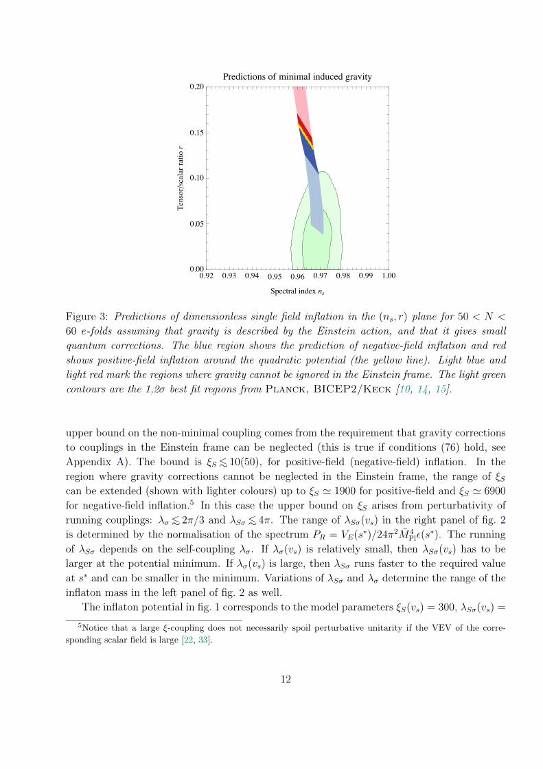
Figure 3: Predictions of dimensionless single field inflation in the (ns, r) plane for 50 < N <

60 e-folds assuming that gravity is described by the Einstein action, and that it gives small

quantum corrections. The blue region shows the prediction of negative-field inflation and red

shows positive-field inflation around the quadratic potential (the yellow line). Light blue and

light red mark the regions where gravity cannot be ignored in the Einstein frame. The light green

contours are the 1,2σ best fit regions from Planck, BICEP2/Keck [10, 14, 15].

upper bound on the non-minimal coupling comes from the requirement that gravity corrections

to couplings in the Einstein frame can be neglected (this is true if conditions (76) hold, see

Appendix A). The bound is ξS <∼ 10(50), for positive-field (negative-field) inflation. In the

region where gravity corrections cannot be neglected in the Einstein frame, the range of ξScan be extended (shown with lighter colours) up to ξS ' 1900 for positive-field and ξS ' 6900

for negative-field inflation.5 In this case the upper bound on ξS arises from perturbativity of

running couplings: λσ <∼ 2π/3 and λSσ <∼ 4π. The range of λSσ(vs) in the right panel of fig. 2

is determined by the normalisation of the spectrum PR = VE(s∗)/24π2M4Plε(s

∗). The running

of λSσ depends on the self-coupling λσ. If λσ(vs) is relatively small, then λSσ(vs) has to be

larger at the potential minimum. If λσ(vs) is large, then λSσ runs faster to the required value

at s∗ and can be smaller in the minimum. Variations of λSσ and λσ determine the range of the

inflaton mass in the left panel of fig. 2 as well.

The inflaton potential in fig. 1 corresponds to the model parameters ξS(vs) = 300, λSσ(vs) =

5Notice that a large ξ-coupling does not necessarily spoil perturbative unitarity if the VEV of the corre-

sponding scalar field is large [22, 33].

12

0.725, λσ(vs) = π/12, yS(vs) = 0.253, yσ(vs) = 0 and msE = 1.28 × 1013 GeV that are in the

physical range, verifying our model independent results in the previous subsection.6 The large

values of the couplings are needed to get a significant deviation from quadratic inflation.

The slow-roll parameters in this model are given by

ε =

[λ′S(s)

λS(s)

]2ξSs

2

2(1 + 6ξS), η =

sξS[λ′S(s) + sλ′′S(s)]

λS(s)(1 + 6ξS), (27)

in terms of which the inflationary parameters are given by

ns = 1− 6ε(s∗) + 2η(s∗), r = 16ε(s∗). (28)

The predictions of dimensionless single field inflation for r as a function of ns are presented in

fig. 3 for 50 < N < 60 [32]. To compare our predictions with experimental results we plot in

the same figure also the contours of the 1,2 σ best-fit regions from the official combination of

the BICEP2/Keck Array/Planck [10, 14, 15].

The yellow line represents the quadratic approximation obtained in the limit β′′λS(vs) = 0

(see eq. (10)). The blue region shows the allowed parameter space for negative-field inflation

and the red region for the positive-field inflation. In the region with darker colours around the

yellow line, the conditions (76) hold and gravity corrections can be neglected in the Einstein

frame. In this region, λσ and λSσ are small and the inflaton potential is well approximated

by (10). The predictions for the inflationary parameters ns and r roughly coincide with the

model-independent predictions. In the light red and light blue regions, the conditions (76) do

not hold, but due to the equivalence of the frames the gravitational corrections in the Einstein

frame must arise from scalar loops in the Jordan frame. The potential is not close to the cubic

(10) any more. We see that for large couplings taking into account exact numerical solutions

for RGE running can induce a large correction in r. For the number of e-folds N = 60, the

lowest possible value of the tensor-to-scalar ratio is r = 0.04.

3 Inflation in agravity

In this section we reconsider inflation within agravity [6]: a renormalizable extension of Einstein

gravity, obtained by adding all dimensionless couplings which are anyhow generated by quantum

corrections, and removing any massive parameter such that power divergences must vanish. The

action has the generic structure

S =

∫d4x√| det g|

[Lmatter −

∑i

ξiϕ2i

2R +

R2

6f 20

+13R2 −R2

µν

f 22

]. (29)

6We choose yσ(vs) = 0 for simplicity. If yσ 6= 0, the predictions for inflation do not change, since its negative

influence on the running of λSσ must be countered by a larger value of λσ in order to get the correct value for

PR.

13

The gravitational kinetic terms suppressed by the dimensionless constants f0 and f2 contain

four derivatives: thereby the graviton contains a massive spin-2 ghost component [34], which

is possibly problematic for energies above its mass M2 = |f2|MPl/√

2: we do not address the

issue of finding a sensible interpretation for it (see [35] for some attempts). In this section, as

mentioned in the introduction, we do not adopt the effective field theory approach of section 2

and eq. (29) is assumed to be the full action, like in ref. [6]. As a curiosity, we notice that the

classical gravitational equations of motion, in a theory with neither matter nor cosmological

constant, have inflationary solutions with arbitrary Hubble constant.

Of course, matter must be present in a realistic theory: a generic Lmatter can be written

in terms of real scalars ϕ, Weyl fermions ψ and vectors Aµ with gauge, Yukawa and quartic

couplings g, y and λ. Furthermore, the scalars ϕi can have dimensionless ξi couplings to gravity.

Once that scalars dynamically get a vacuum expectation value generating the Planck mass as∑i ξiϕ

2i = M2

Pl, agravity realises the scenario of soft-gravity: the graviton splits into the usual

graviton, a massive spin-2 ghost-like graviton and a scalar; their masses M2 an M0 represent

the energy scale at which gravity softens, becoming described by the dimensionless couplings

f2 and f0.

The theory is renormalizable, and quantum corrections enhanced by large logarithms are

taken into account, as usual, by substituting the couplings with running couplings (RGE equa-

tions have been computed in [6]), renormalised at an energy comparable to the energy or field

value of the process under consideration.

3.1 Agravity in the Einstein frame

We want to employ the results in the literature that give the inflationary predictions of multifield

Einstein gravity models. Then, we need to recast the agravity action of eq. (29) in Einstein

form. We here use a compact notation, leaving implicit the sums over the scalars ϕi, which, in a

realistic theory, include at least the Planckion s, the physical Higgs h and the other components

of the Higgs doublet H.

We start adding to the generic agravity Lagrangian the vanishing term−(R + 3f 20χ/2)2/6f 2

0 ,

where χ is an auxiliary field with no kinetic term. Such new term is designed to cancel R2/6f 20 ,

leaving

L =√| det g|

[Lmatter +

13R2 −R2

µν

f 22

− f

2R− 3f 2

0

8χ2

], (30)

where f = χ+ ξϕ2 and7

Lmatter =(Dµϕ)2

2− 1

4F 2µν + ψi /Dψ + (y ϕψψ + h.c.)− V (ϕ). (31)

7If one makes the sum over the scalars ϕi explicit, one should read ξϕ2 as∑i ξiϕ

2i , the kinetic term (Dµϕ)2

as∑iDµϕiDµϕi and so on.

14

Here y denotes a set of Yukawa couplings and V is a general quartic potential. Next, we trans-

form the −fR/2 term into the canonical Einstein term −M2PlRE/2 by performing a rescaling

of the metric,

gEµν = gµν × f/M2Pl. (32)

In the limit of constant f (global scale transformation) our dimensionless action is invariant

provided that the scalars ϕ, the fermions ψ and the vectors Aµ are also rescaled as:

ϕE = ϕ× (M2Pl/f)1/2, ψE = ψ × (M2

Pl/f)3/4, AµE = Aµ. (33)

However, we need to consider a non-constant f and perform a local scale transformation, under

which all dimensionless terms without derivatives remain (trivially) invariant. Furthermore,

various kinetic terms happen to be also (non-trivially) invariant: this is the case for the fermion

kinetic terms [29, 30, 31], the vector kinetic terms and the graviton kinetic term proportional

to 1/f 22 . The scalar kinetic terms are not invariant (away from the special conformal value

ξ = −1/6); thereby we keep using ϕ in addition to ϕE for the scalars. Then the Einstein-frame

Lagrangian is:

L =√

det gE

[ 13R2E −R2

Eµν

f 22

− 1

4F 2Eµν+ψEi /DψE+(yϕEψEψE+h.c.)− M

2Pl

2RE+Lϕ−VE

], (34)

where

Lϕ = M2Pl

[(Dµϕ)2

2f+

3(∂µf)2

4f 2

], VE =

M4Pl

f 2

[V (ϕ) +

3f 20

8χ2

]. (35)

A kinetic term for f has been generated [36], such that f becomes an extra scalar, with

no gauge charge.8 The kinetic metric in scalar field space has constant negative curvature

−Nϕ(Nϕ + 1)M2Pl/6, where Nϕ is the total number of scalars ϕ, and can be conveniently put

in conformal form by redefining z =√

6f , such that our final Lagrangian is

Lϕ =6M2

Pl

z2

(Dµϕ)2 + (∂µz)2

2(36)

and

VE(z, ϕ) =36M4

Pl

z4

[V (ϕ) +

3f 20

8

(z2

6− ξϕϕ2

)2]. (37)

We anticipate here a non-trivial peculiarity of the Einstein-frame Lagrangian, best seen by

considering the case of a single ‘Planckion’ scalar field s, such that f = ξSs2: by using the

first equation in (33) we obtain that sE = MPl/√ξS is a constant i.e. its quartic becomes a

cosmological constant and its Yukawa couplings become fermion mass terms. How can this be

equivalent to the Jordan frame Lagrangian where s has quartic and Yukawa interactions? The

point is that s, being the pseudo-Goldstone boson of spontaneously broken approximate scale

8The scalar kinetic term is conformally invariant for ξϕ = −1/6; this manifests as cancellations in the scalar

kinetic terms.

15

invariance (the explicit breaking of scale invariance coming from the quantum running of the

coupling constants is small because we are assuming perturbative couplings), couples to the

divergence of the dilatation current Dµ, ∂µDµ, that vanishes at tree-level because we consider

special dimensionless theories.9

Mass eigenstates

We compute here the mass eigenstates formed by the scalars φ = h, s, z at the minimum of the

potential, where the scalars kinetic terms of eq. (36) become canonical. Indeed, minimisation

with respect to z leads to z2 = 6M2Pl + 16V/f 2

0 M2Pl. Minimisation with respect to s gives

∂V /∂s− 4ξSsV /M2Pl = 0, that should be solved by M2

Pl =∑ξiϕ

2i ' ξSs

2. The measured value

of the cosmological constant implies a negligible value of V at the minimum, simplifying the

above equations. Minimisation with respect to h then leads to a negligible vacuum expectation

value. On the other hand gauge invariance implies that h should appear at least quadratically

in V ; therefore expanding h around its VEV necessarily produces at least one power of this

negligible VEV, which implies that the Higgs negligibly mixes with s and z. The mass matrix

for the fields s and z around the minimum is given by the second derivatives of VE:

M2s

(1 0

0 0

)+f 2

0 M2Pl

2

(6ξS

√6ξS√

6ξS 1

). (38)

The first term alone would give a Planckion with mass M2s = ∂2V/∂s2. The second term alone

would give a spin-0 graviton with mass M20 = 1

2f 2

0 M2Pl(1 + 6ξS). Taking into account both

terms, the mass eigenvalues are

M2± =

M2s +M2

0

2± 1

2

√(M2

s +M20 )2 − 4

M2sM

20

1 + 6ξS. (39)

3.2 Computing multifield inflationary predictions

The classical equations of motion for the Einstein-frame scalar fields φ = z, s, h during

inflation in slow-roll approximation are

dφ

dN= − z2

6VE

∂VE∂φ

, (40)

having defined the number of e-folds N as dN = H dt. The spin-2 massive graviton does

not affect such classical equations of motion, and we assume that it can be neglected even at

the quantum level. The quantum predictions for inflation can now be computed by using the

previous literature on multifield inflation [37]; they can be expressed in terms of the number of

e-folds starting from a generic initial point, N(h, s, z):

9The explicit verification that the Jordan frame couplings of s vanish on-shell needs manipulations similar to

the ones used to verify the analogous property of the couplings of a Goldstone boson of a U(1) global symmetry,

when a Dirac fermion mass term ΨΨ is re-expressed as derivatives acting within a chiral current Ψγµγ5Ψ.

16

• The power-spectrum of scalar fluctuations is given by

PR(k) =

(H

2π

)2z2

6M2Pl

(∇N)2 (41)

with H computed at horizon exit k = aH and

(∇F )2 ≡(∂F

∂z

)2

+

(∂F

∂s

)2

+

(∂F

∂h

)2

. (42)

• The spectral index ns of scalar perturbations is given by

ns ≡ 1 +d lnPRd ln k

=1

6z2V 2E(∇N)2

6V 2

E

(z2(∇N)2 − 12

)− z4(∇N)2(∇VE)2

+2z3VE

[(∂N

∂h

)2(z∂2VE∂h2

− ∂VE∂z

)+

(∂N

∂z

)2(z∂2VE∂z2

+∂VE∂z

)+2

∂N

∂h

(∂N

∂z

(z∂2VE∂z∂h

+∂VE∂h

)+ z

∂N

∂s

∂2VE∂s∂h

)+ 2

∂N

∂z

∂N

∂s

(z∂2VE∂s∂z

+∂VE∂s

)+

(∂N

∂s

)2(z∂2VE∂s2

− ∂VE∂z

)]. (43)

• The tensor power spectrum is given by Pt(k) = (2/M2Pl)(H/2π)2. Equivalently, the tensor-

to-scalar ratio is given by

r ≡ 4PtPR

=48

z2(∇N)2. (44)

The measured values at k = 0.002 Mpc−1 are PR(k) = (2.14 ± 0.05) × 10−9 [15], ns = 0.965 ±0.006 [13, 15] and r = 0.06± 0.04 (according to [10]) or r = 0± 0.04 (according to [15]).

3.3 Inflationary predictions

In general, predictions of multifield inflation depend on the inflationary trajectory reducing

the predictive power. However, our potential VE(h, s, z) has a peculiar structure, such that

all classical trajectories converge towards a unique attractor solution even when scalar masses

are comparable at the minimum (examples are shown in fig. 4). This presumably happens

because we are considering dimensionless dynamics, such that the derivatives of the potential

are hierarchical almost everywhere in field space. We find that slow-roll inflation starts only

when such attractor is reached. In order to understand our results, it is useful to first consider

three relevant extreme limits:

1. Planckion inflation. If M0 Ms (obtained when the agravity coupling f0 is larger

than the matter couplings in the inflaton sector), the attractor corresponds to z2 ≈ 6ξSs2,

which is the valley along which the squared term proportional to f 20 in VE, eq. (37), nearly

17

N=20

N=20

N=40

N=40

N=60

N=60N=80

N=80

10.3 3

1

10

0.3

3

30

Planckion field sM Pl

Sca

lar

gra

vit

on

fiel

dz

MP

lΞS = 1 , MsM0 = 1.00

ΞS = 1, ΞH = 1 , MsM0 = 0.10, ΛH = 0.01

0

5

10

15

Higgs

hM Pl

12345Planckion sM Pl

5

10

15

zM Pl

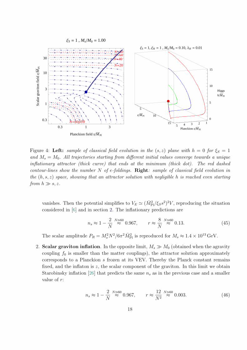
Figure 4: Left: sample of classical field evolution in the (s, z) plane with h = 0 for ξS = 1

and Ms = M0. All trajectories starting from different initial values converge towards a unique

inflationary attractor (thick curve) that ends at the minimum (thick dot). The red dashed

contour-lines show the number N of e-foldings. Right: sample of classical field evolution in

the (h, s, z) space, showing that an attractor solution with negligible h is reached even starting

from h s, z.

vanishes. Then the potential simplifies to VE ' (M2Pl/ξSs

2)2V , reproducing the situation

considered in [6] and in section 2. The inflationary predictions are

ns ≈ 1− 2

N

N≈60≈ 0.967, r ≈ 8

N

N≈60≈ 0.13. (45)

The scalar amplitude PR = M2sN

2/6π2M2Pl is reproduced for Ms ≈ 1.4× 1013 GeV.

2. Scalar graviton inflation. In the opposite limit, Ms M0 (obtained when the agravity

coupling f0 is smaller than the matter couplings), the attractor solution approximately

corresponds to a Planckion s frozen at its VEV. Thereby the Planck constant remains

fixed, and the inflaton is z, the scalar component of the graviton. In this limit we obtain

Starobinsky inflation [26] that predicts the same ns as in the previous case and a smaller

value of r:

ns ≈ 1− 2

N

N≈60≈ 0.967, r ≈ 12

N2

N≈60≈ 0.003. (46)

18

The scalar amplitude PR = f 20N

2/48π2 is reproduced for f0 ≈ 1.8× 10−5.

3. Higgs inflation. We find that, for any value of M0/Ms, inflation is never dominated by

the Higgs, because its quartic self-coupling λH (assumed to be positive) is unavoidably

larger than the other scalar couplings, taking into account its RG running. Even assuming

that the Higgs has a dominant initial vacuum expectation value [21], in our multifield

context inflation starts only after that the field evolution has reached the attractor solution

along which h is subdominant, as exemplified in fig. 4b.

Notice that in both limits 1. and 2. the predictions do not depend on ξS nor on ξH .

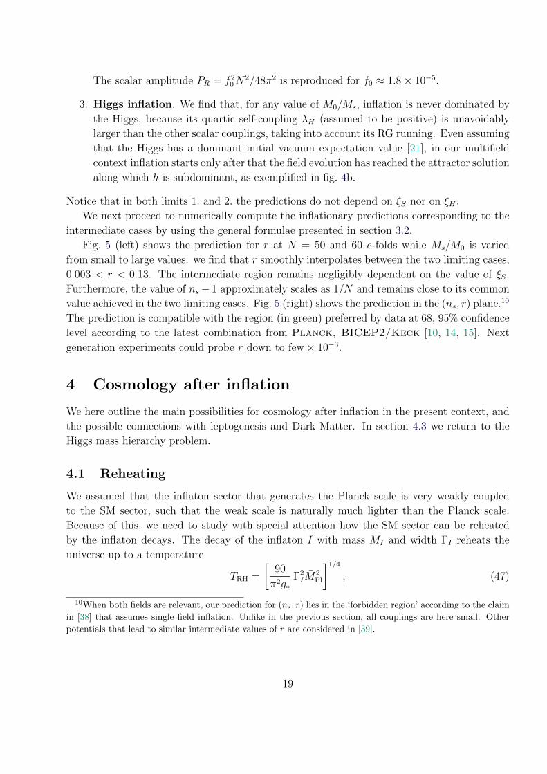
We next proceed to numerically compute the inflationary predictions corresponding to the

intermediate cases by using the general formulae presented in section 3.2.

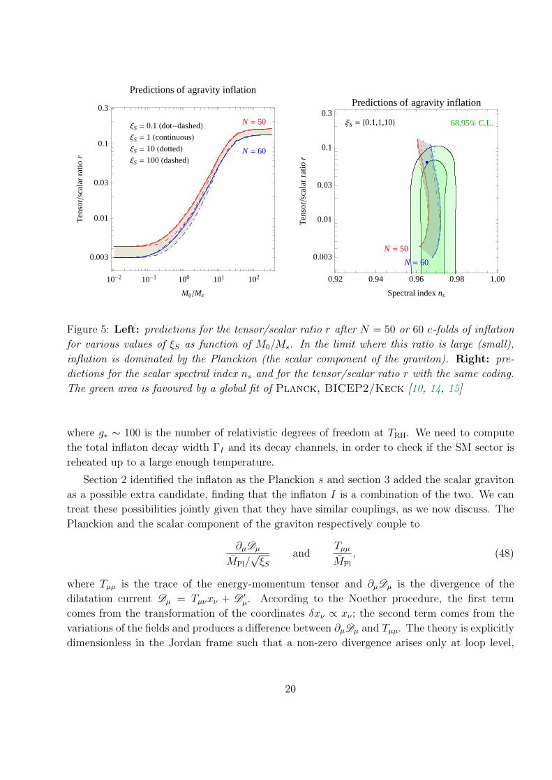
Fig. 5 (left) shows the prediction for r at N = 50 and 60 e-folds while Ms/M0 is varied

from small to large values: we find that r smoothly interpolates between the two limiting cases,

0.003 < r < 0.13. The intermediate region remains negligibly dependent on the value of ξS.

Furthermore, the value of ns− 1 approximately scales as 1/N and remains close to its common

value achieved in the two limiting cases. Fig. 5 (right) shows the prediction in the (ns, r) plane.10

The prediction is compatible with the region (in green) preferred by data at 68, 95% confidence

level according to the latest combination from Planck, BICEP2/Keck [10, 14, 15]. Next

generation experiments could probe r down to few× 10−3.

4 Cosmology after inflation

We here outline the main possibilities for cosmology after inflation in the present context, and

the possible connections with leptogenesis and Dark Matter. In section 4.3 we return to the

Higgs mass hierarchy problem.

4.1 Reheating

We assumed that the inflaton sector that generates the Planck scale is very weakly coupled

to the SM sector, such that the weak scale is naturally much lighter than the Planck scale.

Because of this, we need to study with special attention how the SM sector can be reheated

by the inflaton decays. The decay of the inflaton I with mass MI and width ΓI reheats the

universe up to a temperature

TRH =

[90

π2g∗Γ2IM

2Pl

]1/4

, (47)

10When both fields are relevant, our prediction for (ns, r) lies in the ‘forbidden region’ according to the claim

in [38] that assumes single field inflation. Unlike in the previous section, all couplings are here small. Other

potentials that lead to similar intermediate values of r are considered in [39].

19

10-2 10-1 100 101 102

0.01

0.1

0.003

0.03

0.3

M0Ms

Ten

sors

cala

rra

tio

r

Predictions of agravity inflation

N = 50

N = 60

ΞS = 0.1 Hdot-dashedLΞS = 1 HcontinuousLΞS = 10 HdottedLΞS = 100 HdashedL

0.92 0.94 0.96 0.98 1.00

0.01

0.1

0.003

0.03

0.3

Spectral index ns

Ten

sors

cala

rra

tio

r

Predictions of agravity inflation

ΞS = 80.1,1,10<

N = 50

N = 60

68,95% C.L.

Figure 5: Left: predictions for the tensor/scalar ratio r after N = 50 or 60 e-folds of inflation

for various values of ξS as function of M0/Ms. In the limit where this ratio is large (small),

inflation is dominated by the Planckion (the scalar component of the graviton). Right: pre-

dictions for the scalar spectral index ns and for the tensor/scalar ratio r with the same coding.

The green area is favoured by a global fit of Planck, BICEP2/Keck [10, 14, 15]

where g∗ ∼ 100 is the number of relativistic degrees of freedom at TRH. We need to compute

the total inflaton decay width ΓI and its decay channels, in order to check if the SM sector is

reheated up to a large enough temperature.

Section 2 identified the inflaton as the Planckion s and section 3 added the scalar graviton

as a possible extra candidate, finding that the inflaton I is a combination of the two. We can

treat these possibilities jointly given that they have similar couplings, as we now discuss. The

Planckion and the scalar component of the graviton respectively couple to

∂µDµ

MPl/√ξS

andTµµMPl

, (48)

where Tµµ is the trace of the energy-momentum tensor and ∂µDµ is the divergence of the

dilatation current Dµ = Tµνxν + D ′µ. According to the Noether procedure, the first term

comes from the transformation of the coordinates δxν ∝ xν ; the second term comes from the

variations of the fields and produces a difference between ∂µDµ and Tµµ. The theory is explicitly

dimensionless in the Jordan frame such that a non-zero divergence arises only at loop level,

20

and is given by

∂µDµ =βg1

2g1

Y 2µν +

βg2

2g2

W 2µν +

βg3

2g3

G2µν + βytHQ3U3 + βλH |H|4 + · · · , (49)

where · · · denotes terms beyond the SM and βg = dg/d ln µ is the β function of the coupling

g. The dominant gluon term gives

Γ(I → gg) ≈ |ξS|g43M

3s

(4π)5M2Pl

. (50)

This unavoidable decay channel alone is able of reheating the universe up to

TRH ≈ 107 GeV

(Ms

1013 GeV

)3/2

(51)

for ξS ∼ 1.

The trace of the energy-momentum tensor Tµµ receives the same loop contribution. However,

it also receives a new, possibly dominant, tree-level contribution. Indeed, Tµµ would vanish in

a conformal theory; we are instead considering a non-conformal theory where the ξ couplings

of scalars are generically different from the conformal value ξ = −1/6, as already discussed

around eq. (34). Focusing on the Higgs boson h, the resulting tree-level decay is best computed

by transforming the [(∂µh)2 − ξHh2R]/2 part of the Lagrangian to the Einstein frame and to

canonically normalised fields hE = h× MPl/√f and sE. We find the effective operator11

− (1 + 6ξH)

√ξS

1 + 6ξS

h2E

2

∂2sEMPl

(52)

that produces a tree-level contribution to the decay width

Γ(I → hEhE) = Γ(I → ZZ) =1

2Γ(I → WW ) ≈ (1 + 6ξH)2|ξS|

|1 + 6ξS|M3

I

64πM2Pl

. (53)

The decays to electroweak vectors arise because their longitudinal components are the Goldstone

components of the Higgs doublet H. For ξS,H ∼ 1 this channel gives a TRH ≈ 109 GeV, two

orders of magnitude larger than in eq. (51). However, in section 4.3 we will find that naturalness

of the Higgs mass favours a ξH so close to −1/6 that Γ(I → hEhE) becomes subdominant with

respect to Γ(I → gg).

11A contribution to it was computed in [40].

21

4.2 Dark Matter

So far we neglected possible inflaton decays into the inflaton sector. For example the minimal

model introduced in section 2.2 contains an extra scalar and an extra fermion. Such decays are

not kinematically allowed if the inflaton is the lightest component of its sector. This is the case

in the minimal model, and likely holds more in general, given that the Planckion is the light

pseudo-Goldstone boson of scale invariance.

However, the inflaton sector must contain fermions in order to provide a negative Yukawa

contribution to the β function of the Planckion quartic. Fermions ψ have an associated ψ → −ψsymmetry that keeps the lightest fermion stable.

If the lightest fermion within the inflaton sector has no gauge interactions, then it can also

couple to the SM sector behaving as a right handed neutrino N . It can generate the observed

light neutrino masses via NLH Yukawa couplings [41] (in such a case MN <∼ 107 GeV in order

to avoid an unnaturally large quantum correction to the Higgs mass [42, 4]) and it can provide

baryogenesis via leptogenesis [43].

The lightest fermion in the inflaton sector is instead a stable Dark Matter candidate if

it cannot couple to the SM sector (for example because it has gauge interactions under the

inflaton sector). Assuming that it is light enough to be produced by inflaton decays, it inherits

the observed primordial adiabatic density perturbations.12

The decay width of the inflaton into Dark Matter could be computed along the lines of

eq. (49). A less model-dependent possibility is that such DM fermions get their mass from

another source, independent from the Planckion, that also breaks scale invariance but at a

lower energy scale. Then such fermion masses would contribute to ∂µDµ and to Tµµ as MΨΨ

(we are considering, for example, a Dirac mass term) giving the contribution13

Γ(I → ΨΨ) ≈ |ξS|M2MI

8π(1 + 6ξS)M2Pl

. (54)

By identifying the fermion Ψ with Dark Matter, its abundance is

ΩDM ≡ρDM

ρcr

=s0M

3H20/8πGN

Γ(I → DM)

Γ(I → SM)≈ 0.110

h2× M

0.40 eV

Γ(I → DM)

Γ(I → SM), (55)

having inserted the present entropy density (s0 = gs0T30 2π2/45 with gs0 = 43/11), the present

Hubble constant H0 = h × 100 km/sec Mpc, and the present temperature T0 = 2.725 K. The

observed DM abundance is reproduced for

M ≈ (10− 200) TeV

(MI

1013 GeV

)2/3

. (56)

12An alternative production mechanism can operate even if the fermions are so heavy that decays into them

are not kinematically allowed; however, this alternative would lead to Dark Matter with isocurvature perturba-

tions [44], which are no longer compatible with observations.13The analogous contribution from SM fermion masses is negligible, and the Higgs mass terms Mh would give

a contribution suppressed by two extra powers of Mh/MI .

22

where the lower (higher) estimate applies if Γ(I → gg) (Γ(I → hEhE)) dominates. The

proximity of this mass with the range favoured by the hypothesis that DM is a thermal relic is

an accident: this DM candidate leads to negligible non-gravitational signals in agreement with

present observations.

Finally, we recall that the Higgs potential might be unstable at energies above 1010 GeV [45].

The compatibility of this possible instability with cosmology is discussed in [46].

4.3 Inflation and the weak scale

In models that allow for super-Planckian field variations, inflation becomes a generic natural

phenomenon [8]; however, small parameters are needed to get the observed amplitude of scalar

perturbation PR ≈ 10−9 rather than PR ∼ 1 from chaotic inflation. We obtain a naturally small

PR because we are considering a dimensionless theory with small couplings. Small couplings

are also needed in order to keep the Higgs mass Mh naturally much smaller than MPl. These

models predict a non-trivial connection of the form

Mh ∼ PRMPl (57)

between the weak scale, the Planck scale and the amplitude of inflationary perturbations.

Eq. (57) ignores loop factors (4π)2, e-fold factors N ≈ 60 and the possibility that different

couplings have different size. In the rest of the section we add such factors showing that the

observed Mh/MPl and PR are compatible.

As discussed above, inflation wants f0>∼ 10−5. Thereby, we need to compute the maximal

value of f0 naturally allowed by the Higgs mass.

Whatever sector dynamically breaks scale invariance, it must provide an effective Einstein

term −M2PlR/2. Then, inserting such a term in gravitational loop corrections to the Higgs

propagator, one estimates a correction to the Higgs mass of order

δM2h ∼ ξH

g2(Mg)M2g

(4π)2, (58)

where, as anticipated in section 2, we assume a soft-gravity scenario where new physics at Mg

stops the growth of the gravitational coupling g(E) = E/MPl. Here we are neglecting the

contributions to δM2h proportional to powers of M2

h because they are not dangerous from the

point of view of naturalness. The one-loop effect in (58) is proportional to ξH , the ξ-coupling

that provides interactions between the Higgs and gravity, which do not involve the Higgs mass

or derivatives on the external Higgs field. If ξH vanishes, the correction to M2h arises at two

loops.

Within agravity Mg ∼ M0,M2 and the estimate in eq. (58) gets replaced by a precise

result [6]: the log-enhanced correction to the Higgs mass is described by the following RG

23

equation, valid at energies between MPl and Mg:

(4π)2 d

d ln µ

M2h

M2Pl

= −ξH [5f 42 + f 4

0 (1 + 6ξH)] + · · · , (59)

where µ is the MS renormalization scale and · · · denotes negligible terms. If ξS,H ∼ 1, natural-

ness implies f0<∼ 10−8. This bound can be relaxed by performing a more complete discussion

at the light of the RGE for ξH [6]:

(4π)2 dξHd ln µ

= (1 + 6ξH)

(y2t −

3

4g2

2 −3

20g2

1 + 2λH

)+f 2

0

3ξH(1 + 6ξH)(2 + 3ξH)− 5

3

f 42

f 20

ξH + · · · ,

where · · · denote beyond-the-SM terms. We see that the ξ couplings can naturally acquire two

special values:

• close to zero, ξ ∼ y2/(4π)2, where y is a generic coupling of the theory, e.g. y ∼ yt in the

SM;

• close to the conformal value, ξ + 1/6 ∼ f 42 /(4πf0)2.

In the latter case, the larger f0 ∼ 10−5 called by inflation becomes naturally allowed. We thereby

conclude that the smallness of Mh/MPl and the smallness of PR are mutually compatible,

although the ξ terms need to lie in special natural ranges.

5 Conclusions

We computed the inflationary predictions of models where mass scales (in particular the Planck

scale) are absent at tree-level and generated only by quantum corrections from dimensionless

dynamics. The same sector that generates the Planck mass does also provide cosmological

inflation with super-Planckian field variations: the slow-roll parameters are related to the β-

functions of the theory. We consider two scenarios: single field inflation in an effective field

theory approach, and inflation in agravity, which is a UV completion of general relativity

coupled to the SM fields.

In the first case, in the limit where couplings are small enough that gravity effects can be

ignored in the Einstein frame, we showed the consistency between computations in the Jordan

and in the Einstein frames, obtaining an inflaton potential which is approximatively quadratic

with a cubic correction, leading to

ns ≈ 0.967, r ≈ 0.13. (60)

If, instead, ξS and other couplings are large one can obtain smaller values of r, down to about

0.04, as shown in fig. 3.

In the second case, we considered agravity, the dimensionless extension of Einstein gravity

that allows, for small enough couplings, the natural co-existence of the small weak scale with

24

the much larger Planck scale MPl even in absence of new physics at the weak scale. Agravity

implies an extra scalar component of the graviton and an extra spin-2 ghost-like graviton that

make quantum gravity renormalizable and controlled by two dimensionless couplings f0, f2.

A small amplitude of scalar perturbations is also predicted because this sector must contain

small couplings such that the weak scale Mh/MPl is naturally small, resulting in a relation that

scales as PR ∼Mh/MPl, more precisely discussed in section 4.3. We computed the inflationary

predictions finding the result in fig. 5 (right):

ns ≈ 0.967, 0.003 < r < 0.13, (61)

which agrees with present observations. Fig. 5 (left) shows that the upper range of r is realised

if the ‘Higgs of gravity’ is the lighter scalar that dominates inflation (this limit gives the ef-

fective field theory scenario discussed above); the lower range is realised if instead the lighter

inflationary field is the scalar component of the graviton.

Both in the effective field theory and in agravity, the inflaton decays via Planck-suppressed

interactions (it couples to a combination of the trace of the energy momentum tensor and of

the divergence of the dilatation current) producing a reheating temperature TRH ∼ 107−9 GeV.

Furthermore the inflation sector must contain fermions that either behave as right-handed

neutrinos (if they have no gauge interactions) or are stable. In the latter case, they might

be light enough that the inflaton can decay in them, providing the observed Dark Matter

abundance with adiabatic primordial inhomogeneities if their mass is around 10− 200 TeV.

A determination of the tensor-to-scalar ratio r in the future can help us to discriminate

between different paradigms behind inflation and to test quantum theories of gravity such as

agravity.

Acknowledgments

We thank Juan Garcıa-Bellido, Mario Herrero-Valea and Hardi Veermae for useful discussions.

This work was supported by grants PUT799, MTT8, MTT60, IUT23-6, CERN+, and by EU

through the ERDF CoE program. The work of Alberto Salvio has been also supported by the

Spanish Ministry of Economy and Competitiveness under grant FPA2012-32828, Consolider-

CPAN (CSD2007-00042), the grant SEV-2012-0249 of the “Centro de Excelencia Severo Ochoa”

Programme and the grant HEPHACOS-S2009/ESP1473 from the C.A. de Madrid.

A RGE and the compatibility of frames

In this Appendix we give more details about the compatibility between computations performed in

the Jordan and Einstein frame in the effective field theory approach described in Section 2. This is

particularly relevant since we have to make sure that the RG running in the Jordan frame and in the

Einstein frame is consistent.

25

It has been shown that the results computed in the Jordan and Einstein frames are compatible

with each other [49]. However, according to the problem at hand, computations can be easier in one

frame or another. Usually it is easier to compute the RGEs in the Jordan frame, while inflationary

calculations are more simply performed using standard formulæ valid in the Einstein frame. The

RGEs of the Jordan frame can be applied to Einstein frame once we keep in mind that also the

renormalisation scale has to rescale under a Weyl transformation [49]. In order to fully recover the

equivalence one would need to include gravitational loops, that we neglect.

Let us consider the minimal model described by the Lagrangian (17) in the Jordan frame. Assuming

the possibility to neglect quantum gravity corrections eq. (11), the one-loop level β-functions for the

couplings in the Jordan frame are given by

16π2βλS = 18λ2S +

1

2λ2Sσ + 4λSy

2S − 4y4

S , (62)

16π2βλσ = 18λ2σ +

1

2λ2Sσ + 4λσy

2σ − 4y4

σ, (63)

16π2βλSσ = 4λ2Sσ + 6λSσ(λS + λσ) + 4λSσ(y2

S + y2σ)− 24y2

Sy2σ, (64)

16π2βyS = 4yS(y2S + y2

σ), (65)

16π2βyσ = 4yσ(y2S + y2

σ), (66)

16π2βξS =

(ξS +

1

6

)(6λS +

1

6y2S

). (67)

We used the PyR@TE package [47] to derive the RGEs for the scalar and Yukawa couplings and Ref.

[48] for the non-minimal coupling ξS . On the other hand, in the approximation of weakly coupled

gravity, the RGEs for the parameters of the Einstein frame Lagrangian (18) are

16π2βΛ =1

2m4σ −m4

ψ, (68)

16π2βλσ = 18λ2σ + 4λσy

2σ − 4y4

σ, (69)

16π2βm2σ

= (6λσ + 4y2σ)m2

σ − 24y2σm

2ψ, (70)

16π2βmψ = 4y2σmψ, (71)

16π2βyσ = 4y3σ, (72)

where the connection between the Jordan and Einstein frame parameters is given by

Λ =1

4

λSξ2S

M4Pl, (73)

m2σ =

1

2

λSσξS

M2Pl, (74)

mψ =yS√ξSMPl. (75)

We see that the RGEs are not perfectly matching with each other. This is because we neglect gravita-

tional corrections due to the mixing of gravitational and scalar degrees of freedom in the transformation

between the frames. To match the RGEs of the Jordan frame and the RGEs of Einstein frame in the

weak gravity limit, we need to impose

λS λSσ λσ, βyS yS , βξS ξS , (76)

26

on the Jordan frame parameters. However, since physical observables are frame independent [49], the

quantum gravity corrections in the Einstein frame must be reproduced by scalar loops in the Jordan

frame.

References

[1] CMS Collaboration, Phys. Lett. B 716 (2012) 30 [arXiv:1207.7235].

[2] ATLAS Collaboration, Phys. Lett. B 716 (2012) 1 [arXiv:1207.7214].

[3] See presentations at the conferences “Nature guiding Theory” (FermiLab, August 2014) and “Rethinking

Naturalness” (FrascatiLab, Rome, December 2014).

[4] M. Farina, D. Pappadopulo and A. Strumia, JHEP 1308, 022 (2013) [arXiv:1303.7244]. M. Heikin-

heimo, A. Racioppi, M. Raidal, C. Spethmann, K. Tuominen, Mod. Phys. Lett. A 29 (2014) 1450077

[arXiv:1304.7006]. A. de Gouvea, D. Hernandez and T. M. P. Tait, Phys. Rev. D 89 (2014) 115005

[arXiv:1402.2658].

[5] W Bardeen, FERMILAB-CONF-95-391-T. C. T. Hill, arXiv:hep-th/0510177. R. Hempfling, Phys. Lett.

B 379 (1996) 153 [arXiv:hep-ph/9604278]. R. Foot, A. Kobakhidze and R. R. Volkas, Phys. Lett. B 655

(2007) 156 [arXiv:0704.1165]. R. Foot, A. Kobakhidze, K.L. McDonald and R.R. Volkas, Phys. Rev. D

76 (2007) 075014 [arXiv:0706.1829]. R. Foot, A. Kobakhidze, K.L. McDonald, R.R. Volkas, Phys. Rev. D

77 (2008) 035006 [arXiv:0709.2750]. M. Shaposhnikov and D. Zenhausern, Phys. Lett. B 671 (2009) 187

[arXiv:0809.3395]. M. Shaposhnikov and D. Zenhausern, Phys. Lett. B 671 (2009) 162 [arXiv:0809.3406].

M. E. Shaposhnikov and I. I. Tkachev, Phys. Lett. B 675 (2009) 403 [arXiv:0811.1967]. S. Iso, N. Okada and

Y. Orikasa, Phys. Lett. B 676 (2009) 81 [arXiv:0902.4050]. L. Alexander-Nunneley and A. Pilaftsis, JHEP

1009 (2010) 021 [arXiv:1006.5916]. T. Hur and P. Ko, Phys. Rev. Lett. 106 (2011) 141802 [arXiv:1103.2571].

D. Blas, M. Shaposhnikov and D. Zenhausern, Phys. Rev. D 84 (2011) 044001 [arXiv:1104.1392]. C. En-

glert, J. Jaeckel, V. V. Khoze and M. Spannowsky, JHEP 1304 (2013) 060 [arXiv:1301.4224]. E. J. Chun,

S. Jung and H. M. Lee, Phys. Lett. B 725 (2013) 158 [arXiv:1304.5815]. M. Heikinheimo, A. Racioppi,

M. Raidal, C. Spethmann and K. Tuominen, Nucl. Phys. B 876 (2013) 201 [arXiv:1305.4182]. T. Ham-

bye, A. Strumia, Phys. Rev. D 88 (2013) 055022 [arXiv:1306.2329]. A. Farzinnia, H. J. He and J. Ren,

Phys. Lett. B 727 (2013) 141 [arXiv:1308.0295]. C. D. Carone and R. Ramos, Phys. Rev. D 88, 055020

(2013) [arXiv:1307.8428]. V. V. Khoze, JHEP 1311 (2013) 215 [arXiv:1308.6338]. E. Gabrielli, M. Heik-

inheimo, K. Kannike, A. Racioppi, M. Raidal and C. Spethmann, Phys. Rev. D 89 (2014) 1, 015017

[arXiv:1309.6632]. T. G. Steele, Z. W. Wang, D. Contreras and R. B. Mann, Phys. Rev. Lett. 112

(2014) 17, 171602 [arXiv:1310.1960]. M. Hashimoto, S. Iso and Y. Orikasa, Phys. Rev. D 89 (2014)

1, 016019 [arXiv:1310.4304]. M. Holthausen, J. Kubo, K. S. Lim and M. Lindner, JHEP 1312 (2013)

076 [arXiv:1310.4423]. I. Quiros, arXiv:1312.1018, arXiv:1401.2643. S. Benic and B. Radovcic, Phys. Lett.

B 732 (2014) 91 [arXiv:1401.8183]. J. Kubo, K. S. Lim and M. Lindner, Phys. Rev. Lett. 113 (2014)

091604 [arXiv:1403.4262]. J. Kubo, K. S. Lim and M. Lindner, JHEP 1409 (2014) 016 [arXiv:1405.1052].

S. Benic and B. Radovcic, arXiv:1409.5776. W. Altmannshofer, W. A. Bardeen, M. Bauer, M. Carena and

J. D. Lykken, arXiv:1408.3429. O. Antipin, M. Redi and A. Strumia, arXiv:1410.1817.

[6] A. Salvio and A. Strumia, JHEP 1406 (2014) 080 [arXiv:1403.4226].

[7] K. Kannike, A. Racioppi and M. Raidal, JHEP 1406 (2014) 154 [arXiv:1405.3987].

[8] A. H. Guth, Phys. Rev. D 23 (1981) 347. A. D. Linde, Phys. Lett. B 108 (1982) 389. A. Albrecht and

P. J. Steinhardt, Phys. Rev. Lett. 48 (1982) 1220.

27

[9] V. F. Mukhanov and G. V. Chibisov, JETP Lett. 33 (1981) 532 [Pisma Zh. Eksp. Teor. Fiz. 33 (1981)

549]. J. M. Bardeen, P. J. Steinhardt and M. S. Turner, Phys. Rev. D 28 (1983) 679. V. F. Mukhanov,

H. A. Feldman and R. H. Brandenberger, Phys. Rept. 215 (1992) 203.

[10] BICEP2/Keck and Planck Collaborations, arXiv:1502.00612.

[11] Planck Collaboration, arXiv:1409.5738.

[12] BICEP2 Collaboration, Phys. Rev. Lett. 112 (2014) 24, 241101 [arXiv:1403.3985].

[13] Planck Collaboration, Astron. Astrophys. 571 (2014) A22 [arXiv:1303.5082].

[14] P. A. R. Ade et al. [BICEP2 and Keck Array Collaborations], [arXiv:1502.00643].

[15] Planck Collaboration, arXiv:1502.01589. P. A. R. Ade et al. [Planck Collaboration], arXiv:1502.02114.

[16] S. Hotchkiss, A. Mazumdar and S. Nadathur, JCAP 1202 (2012) 008 [arXiv:1110.5389]. A. Chatterjee and

A. Mazumdar, arXiv:1409.4442.

[17] P. Minkowski, Phys. Lett. B 71 (1977) 419. A. Zee, Phys. Rev. Lett. 42 (1979) 417. S.L. Adler, Phys. Rev.

Lett. 24 (1980) 1567. C. Wetterich, Nucl. Phys. B 302 (1988) 668. C. Wetterich, Phys. Rev. Lett. 90 (2003)

231302 [arXiv:hep-th/0210156]. C. Lin, arXiv:1405.4821.

[18] J. R. Ellis, D. V. Nanopoulos, K. A. Olive and K. Tamvakis, Phys. Lett. B 120 (1983) 331. A. D. Linde,

Phys. Lett. B 114 (1982) 431. J. R. Ellis, D. V. Nanopoulos, K. A. Olive and K. Tamvakis, Nucl. Phys. B

221 (1983) 524.

[19] S. R. Coleman and E. J. Weinberg, Phys. Rev. D 7 (1973) 1888.

[20] C. D. Froggatt and H. B. Nielsen, Phys. Lett. B 368 (1996) 96 [arXiv:hep-ph/9511371].

[21] F. L. Bezrukov and M. Shaposhnikov, Phys. Lett. B 659 (2008) 703 [arXiv:0710.3755].

[22] F. Bezrukov, A. Magnin, M. Shaposhnikov and S. Sibiryakov, JHEP 1101 (2011) 016 [arXiv:1008.5157].

[23] T. Futamase and K. I. Maeda, Phys. Rev. D 39 (1989) 3. D. S. Salopek, J. R. Bond and J. M. Bardeen,

Phys. Rev. D 40 (1989) 1753. N. Makino and M. Sasaki, Prog. Theor. Phys. 86 (1991) 103. R. Fakir,

S. Habib and W. Unruh, Astrophys. J. 394 (1992) 396. E. Komatsu and T. Futamase, Phys. Rev. D 59

(1999) 064029 [arXiv:astro-ph/9901127].

[24] D. H. Lyth, Phys. Rev. Lett. 78 (1997) 1861 [arXiv:hep-ph/9606387]. For the recent update and references

see, S. Antusch and D. Nolde, JCAP 1405 (2014) 035 [arXiv:1404.1821].

[25] A. D. Linde, Phys. Lett. B 129 (1983) 177.

[26] A. A. Starobinsky, Phys. Lett. B91 (1980) 99.

[27] G. F. Giudice, G. Isidori, A. Salvio and A. Strumia, arXiv:1412.2769.

[28] Y. Hamada, H. Kawai and K. y. Oda, JHEP 1407 (2014) 026 [arXiv:1404.6141].

[29] K. Hayashi, M. Kasuya and T. Shirafuji, Prog. Theor. Phys. 57 (1977) 431 [Erratum-ibid. 59 (1978) 681].

[30] See e.g. Y. Fuji, K. Maeda, “The Scalar-Tensor Theory of Gravitation”, appendix F.

[31] Y. Watanabe and E. Komatsu, Phys. Rev. D 75 (2007) 061301 [arXiv:gr-qc/0612120].

[32] See e.g. A. R. Liddle and S. M. Leach, Phys. Rev. D 68 (2003) 103503 [arXiv:astro-ph/0305263]. L. Dai,

M. Kamionkowski and J. Wang, Phys. Rev. Lett. 113 (2014) 041302 [arXiv:1404.6704]. J. B. Munoz and

M. Kamionkowski, arXiv:1412.0656.

[33] G. F. Giudice and H. M. Lee, Phys. Lett. B 694 (2011) 294 [arXiv:1010.1417].

28

[34] K. S. Stelle, Phys. Rev. D 16 (1977) 953.

[35] E. Tomboulis, Phys. Lett. B 70 (1977) 361. A. Salam and J. A. Strathdee, Phys. Rev. D 18 (1978)

4480. S. L. Adler, Phys. Lett. B 95 (1980) 241. B. Hasslacher and E. Mottola, Phys. Lett. B 99 (1981) 221.

E. Tomboulis, Phys. Lett. B 97 (1980) 77. I. Antoniadis and E. T. Tomboulis, Phys. Rev. D 33 (1986) 2756.

S. W. Hawking and T. Hertog, Phys. Rev. D 65 (2002) 103515 [arXiv:hep-th/0107088]. P. D. Mannheim,

Found. Phys. 42 (2012) 388 [arXiv:1101.2186].

[36] See e.g. D. I. Kaiser, Phys. Rev. D 81 (2010) 084044 [arXiv:1003.1159].

[37] See e.g. A. A. Starobinsky, JETP Lett. 42 (1985) 152 [Pisma Zh. Eksp. Teor. Fiz. 42 (1985) 124]. L. A. Kof-

man and D. Y. Pogosian, Phys. Lett. B 214 (1988) 508. J. Garcia-Bellido and D. Wands, Phys. Rev. D

52 (1995) 6739 [arXiv:gr-qc/9506050]. M. Sasaki and E. D. Stewart, Prog. Theor. Phys. 95 (1996) 71

[arXiv:astro-ph/9507001]. J. Garcia-Bellido and D. Wands, Phys. Rev. D 53 (1996) 5437 [arXiv:astro-

ph/9511029]. T. Chiba and M. Yamaguchi, JCAP 0901 (2009) 019 [arXiv:0810.5387].

[38] D. Roest, JCAP 1401 (2014) 01, 007 [arXiv:1309.1285]. B. J. Broy, D. Roest and A. Westphal,

arXiv:1408.5904. P. Creminelli, S. Dubovsky, D. L. Nacir, M. Simonovic, G. Trevisan, G. Villadoro and

M. Zaldarriaga, arXiv:1412.0678.

[39] R. Kallosh, A. Linde and D. Roest, JHEP 1311 (2013) 198 [arXiv:1311.0472]. K. Nozari and S. D. Sadatian,

Mod. Phys. Lett. A 23 (2008) 2933 [arXiv:0710.0058]. N. Okada, M. U. Rehman and Q. Shafi, Phys. Rev.

D 82 (2010) 043502 [arXiv:1005.5161]. N. Okada, V. N. Senoguz and Q. Shafi, arXiv:1403.6403.

[40] C. Csaki, N. Kaloper, J. Serra and J. Terning, Phys. Rev. Lett. 113 (2014) 161302 [arXiv:1406.5192].

[41] P. Minkowski, Phys. Lett. B67 (1977) 421.

[42] F. Vissani, Phys. Rev. D 57 (1998) 7027 [arXiv:hep-ph/9709409].

[43] M. Fukugita and T. Yanagida, Phys. Lett. B 174, 45 (1986). A precise computation was performed in

G. F. Giudice, A. Notari, M. Raidal, A. Riotto and A. Strumia, Nucl. Phys. B 685 (2004) 89 [arXiv:hep-

ph/0310123].

[44] V. Kuzmin and I. Tkachev, Phys.Rev. D59 (1999) 123006 [arXiv:hep-ph/9809547].

[45] For a precise computation see D. Buttazzo, G. Degrassi, P. P. Giardino, G. F. Giudice, F. Sala, A. Salvio

and A. Strumia, JHEP 1312 (2013) 089 [arXiv:1307.3536].

[46] J.R. Espinosa et al., arXiv:1505.04825.

[47] F. Lyonnet, I. Schienbein, F. Staub, A. Wingerter, Comput. Phys. Commun. 185 (2014) 1130

[arXiv:1309.7030].

[48] M. Herranen, T. Markkanen, S. Nurmi, A. Rajantie, Phys. Rev. Lett. 113 (2014) 21 [arXiv:1407.3141].

[49] D. P. George, S. Mooij and M. Postma, JCAP 1402 (2014) 024 [arXiv:1310.2157]. M. Postma and

M. Volponi, Phys. Rev. D 90 (2014) 10, 103516 [arXiv:1407.6874].

29