Embed Size (px)
Citation preview

The University of MaineDigitalCommons@UMaine
Electronic Theses and Dissertations Fogler Library
2002
Dynamic Response of a Mobile Offshore BaseHydroelastic Test ModelVijay Venkataraman
Follow this and additional works at: http://digitalcommons.library.umaine.edu/etd
Part of the Mechanical Engineering Commons
This Open-Access Thesis is brought to you for free and open access by DigitalCommons@UMaine. It has been accepted for inclusion in ElectronicTheses and Dissertations by an authorized administrator of DigitalCommons@UMaine.
Recommended CitationVenkataraman, Vijay, "Dynamic Response of a Mobile Offshore Base Hydroelastic Test Model" (2002). Electronic Theses andDissertations. 313.http://digitalcommons.library.umaine.edu/etd/313

DYNAMIC RESPONSE OF A MOBILE OFFSHORE BASE
HYDROELASTIC TEST MODEL
BY
Vijay Venkataraman
B.S. University of Maine, 1998
A THESIS
Submitted in Partial Fulfillment of the
Requirements for the Degree of
Master of Science
(in Mechanical Engineering)
The Graduate School
The University of Maine
August, 2001
Advisory Committee:
Vincent Caccese, Associate Professor of Mechanical Engineering, Advisor
Donald Grant, Chair and R.C. Hill Professor of Mechanical Engineering
Richard Sayles, Associate Professor of Mechanical Engineering

LIBRARY RIGHTS STATEMENT
In presenting this thesis in partial fulfillment of the requirements for an advanced
degree at The University of Maine, I agree that the Library shall make it fieely
available for inspection. I further agree that permission for "fair use" copying of this
thesis for scholarly purposes may be granted by the Librarian. It is understood that
any copying or publication of this thesis for financial gain shall not be allowed without
my written permission.
Date: 8 123 lo\

DYNAMIC RESPONSE OF A MOBILE OFFSHORE BASE
HYDROELASTIC TEST MODEL
By Vijay Venkataraman
Thesis Advisor: Dr. Vincent Caccese
An Abstract of the Thesis Presented in Partial Fulfillment of the Requirements for the
Degree of Master of Science (in Mechanical Engineering)
August, 2001
The objective of the work presented in this thesis deals with the study of dynamic
response of a Mobile Offshore Base (MOB) hydroelastic test model. The MOB is a
very large floating structure consisting of multiple self-propelled, semi-submersible
modules. Physical scale model testing of a notional MOB concept has been conducted
and the experimental results have been provided for one, two and four module
configurations. This thesis focuses on utilizing the experimental data to understand the
dynamic response of the MOB hydroelastic scale module. The analysis of the data is
conducted using popular linear and nonlinear data processing techniques. The
objectives are to obtain the modal shapes of the dynamic response, investigate the
effect of connector dynamics in multi-module scale models and determine the
nonlinear characteristics of the response.

The results of this study suggest that the MOB module acts as an elastic
structure. Single module configurations show good heave, pitch and surge response
under head seas and include a good roll response under quartering seas. Torsion of the
module is also observed under quartering seas for the single module. The single
module configurations also show the development of a nonlinear damping force. The
two and four module configurations show both in-phase and out-of-phase response
characteristics between the interconnected modules constrained rigidly by the
connectors.

The author would like to thank Dr. Vincent Caccese for being a very supportive
graduate advisor. The author would also like to acknowledge the assistance of Eric
Weybrant, HKS, Robert Coppolino, MA Corp, Richard Lewis, NSWCCD, and Dr.
Senthil Vel, University of Maine. The assistance of research engineer Keith Berube,
several graduate and undergraduate students, including Jean-Paul Kabche, Albert
Davila, Chris Malm, Joshua Walls, Randy Bragg, and Mike Boone is greatly
appreciated. The assistance of Arthur Pete, the manager of the University of Maine
Crosby Laboratories, and department administrative assistant Sheryl Brockett is also
appreciated. The author would like to thank the Office of Naval Research for their
generous funding which paid for a large portion of the author's graduate education.
Also, the author would like to thank the members of his graduate committee, Dr. :,
Donald Grant, and Dr. Richard Sayles, and the graduate student coordinator Dr.
Michael Peterson for their input and support. Finally, the author would like to thank
his parents, sister and fiends at the University of Maine for their support.

TABLE OF CONTENTS
. . ACKNOWLEDGEMENTS ....................................................................... 11 LIST OF TABLES .................................................................................. vii
... LIST OF FIGURES ................................................................................. viii
Chapter
1 INTRODUCTION ........................................................................... 1
1.1 Physical Scale Model Tests .......................................................... 3
1.2 Objective ............................................................................... 5
1.3 Scope of Work ........................................................................... 6
2 FLUID-STRUCTURE INTERACTION AND WAVE THEORY .............. 7
2.1 Fundamentals ............................................................................ 7
2.2 Fluid-Structure Interaction - Basic Vortex Theory ............................ 8
2.2.1 Effect of Cylinder Motion on Wake of Vortex
Induced Vibration ................................................................ 9
2.2.2 Vortex Induced Oscillations - Models .................................... 10
2.2.2.1 Wake Oscillator Model (Cylindrical Structures Only) .......... 10
2.2.2.2 Correlation Model (Right Circular Cylinder) ................... 12
2.2.3 Reduction of Vortex-Induced Vibration ................................... 13
2.3 Basic Structural Vibration ............................................................ 14
2.3.1 Basic Vibration Definitions ................................................... 14
2.3.1.1 Spring Stiffness .......................................................... 14
2.3.1.2 Natural Frequency of Vibration ...................................... 14
2.3.2 Vibrational Damping .......................................................... 15
2.4 Added Mass Effect ..................................................................... 17
2.4.1 Added Mass or the Inertial Mass of the Entrained Fluid .............. 17
2 .4.2 Added Mass Moment of Inertia ............................................. 19
2.4.3 Added Damping ................................................................. 19
2.5 Vibrations Induced by an Oscillating Flow ..................................... 20 . .
2.6 Ship Motion in a Seaway ............................................................. 21

....................................................................... 2.6.1 Introduction 2 1
............................................................................ 2.6.2 Stability 23
............................................................ 2.6.3 Natural Frequencies -24
............................................. 2.6.3.1 Natural Frequency of Roll 24
............................................ 2.6.3.2 Natural Frequency of Pitch 25
.......................................... 2.6.3.3 Natural Frequency of Heave 26
................................................... 2.7 Sea Waves and Wave Spectrums 27
...................................................... 2.7.1 Sea State Representation 27
............................................................ 2.7.2 Linear Wave Theory 28
................................................................... 2.7.3 Wave Loading 29
................................................................. 2.7.4 Wave Spectrums 30 . . ................................................................ 2.7.5 Wave Conditions 32
3 PHYSICAL SCALE MODEL, DATA REDUCTION, AND
................................................... VISUALIZATION TECHNIQUE 34
.................................................................. 3.1 Physical Scale Model 34
3.1.1 Wave Tank ........................................................................ 35
3.1.2 Hull Form .......................................................................... 36
................................................................ 3.1.3 Internal Structure 37
.................................................................. 3.1.4 End Connectors 40
.......................................................................... 3.1.5 Ballasting 40
.................................................................. 3.1.6 Instrumentation 41
........................................................................... 3.2 Data Reduction 42
................................... 3.2.1 Differentiation and Integration Scheme 44
.................................................. 3.2.2 Noise Removal (Filtration) 45 . . .............................................................. 3.3 Visual~zation Technique 48
4 FREQUENCY RESPONSE FUNCTIONS, SUSO AND MUSO
............................................................................ ANALYSIS 50
..................................................... 4.1 Frequency Response Functions 50
............................................................ 4.1.1 Coherence Function 53
4.1.2 Phase ............................................................................... 55

4.2 SVSO & MVSO Analysis ............................................................. 55
4.2.1 Linear SVSO Model ............................................................ 58
4.2.2 Nonlinear MVSO Model ....................................................... 61
4.2.2.1 Direct MIISO Nonlinear Model ...................................... 61
4.2.2.2 Reverse MVSO Nonlinear Model ................................... 66
4.3 SVSO and MVSO analysis using the ITAP MATLAB
Toolbox ................................................................................... 71
ANALYSIS OF SINGLE MODULE MOB SCALE MODEL .................. 75
5.1 SVSO Analysis - Comparison between DynamicData
and ITAPTM ............................................................................. 77
5.2 Results of Analysis of a Single Module MOB Scale Model ................ 80
5.2.1 Results for OCHI Head Sea 2-50per 900 RPM Data Set ............. 81
5.2.2 Results for Bretschneider BOW66 (b) Quartering Sea
2-58per 1 125 RPM Data Set .................................................. 91
ANALYSIS OF TWO AND FOUR MODULE MOB SCALED MODEL ... 101
6.1 Analysis of OCHI 1 100 RPM Head Sea Two Module Data Set ............ 101
6.2 Analysis of Bretschneider 1125 RPM 85DEG Quartering Sea
Four Module Data Set ................................................................. 1 1 1
SUMMARY, CONCLUSIONS, AND FUTURE WORK ....................... 120
7.1 Summary .................................................................................. 120
7.2 Conclusions ............................................................................... 120
7.3 Future Work .............................................................................. 121
BIBLIOGRAPHY ................................................................................... 123
Appendix A Non-Dimensional Parameters of a Two.Dimensiona1.
Spring.Supported. Damped Structural Model Exposed
to a Steady Flow .................................................................. 126
Appendix B Wave Spectrums ................................................................. 130

Appendix C Differentiation and Integration Functions . MATLAB . . Code Listing .................................................................. 132
Appendix D Time History. SYSO and MYSO Results for Single Module
MOB Scale Model Test .......................................................... 135
Appendix E Scaling Issue with the Four Module Acceleration Data .................. 157
BIOGRAPHY OF THE AUTHOR ......................................................... 160
LIST OF TABLES
Table 5.1 :
Table 5.2:
Table 5.3:
Table 5.4:
Table 5.5:
Table 5.6:
Table 5.7:
Table 6.1 :
Table 6.2:
Table 6.3:
Single Module MOB Data Sets Analyzed ...............................
Summary of the Analyzed Hydrodynamic Data Channel
Designations ..............................................................
MVSO Models Applied to the Data Sets ................................
Summary of Results for the OCHI Single Module ....................
SVSO and MVSO Results for the OCHI Single Module MOB ....
Summary of Results for the Bretschneider Single Module .........
SVSO and MVSO Results for the Bretschneider Single Module
MOB ..............................................................................
Channel Designations in the OCHI Two Module Data Set .........
Summary of Results for OCHI Two Module MOB ..................
Channel Designations in the Bretschneider Quartering Sea
Data ............................................................................... 111
Table 6.4: Summary of Results for Bretschneider Four Module MOB Data
Set ................................................................................ 115
vii

LIST OF FIGURES
Figure 1.1 :
Figure 1.2:
Figure 2.1 :
Figure 2.2:
Figure 2.3:
Figure 2.4:
Figure 2.5:
Figure 3.1 :
Figure 3.2:
Figure 3.3:
Figure 3.4:
Figure 3.5:
Figure 3.6:
Figure 3.7:
Figure 3.8:
Figure 3.9:
Figure 4.1 :
Figure 4.2:
McDermott Shipping. Inc . MOB Concept .....................
Nominal MOB Semi.Submersibles ..............................
Stability of Ship in Roll .............................................
Schematic Representation of a Simple Harmonic
.................................................................... Wave
Bredschneider Double Height Spectra .........................
OCHI Six-Parameter Spectrum ..................................
Three Unidirectional Random Seas .............................
Scale Model Test ....................................................
...................................... NSWC MASK Test Facility
MOB Structural Model .............................................
MOB Connector .....................................................
Location of tri-axial accelerometers ............................
DynamicData Program ............................................
Constant Acceleration Method of Integration ..............
Noise Filtration Technique ......................................
MOB-Animate Animation Program ..........................
Sample FRF for a SVSO Function ............................
Coherence Function for a SIISO FRF shown in
Figure 4.1 ......................................................
viii

Figure 4.3:
Figure 4.4:
Figure 4.5:
Figure 4.6:
Figure 4.8:
Figure 4.9:
Figure 4.10:
Figure 4.1 1 :
Figure 5.1:
Figure 5.2:
Figure 5.3:
Figure 5.4:
Figure 5.5:
Figure 5.6:
Figure 5.7:
Phase Function for a SUSO FRF .............................
Six-DOF Sea Motion ............................................
Reverse Dynamic Single-Input/Single-Output system .....
Direct Dynamic Single-Input/Single-Output Linear
................................................................... Model
Direct Dynamic Two-Input/Single-Output Linear
Model ...................................................................
Direct Dynamic Three-Input/Single-Output Linear
Model ....................................................................
Reverse Dynamic Two-Input/Single-Output Linear
.................................................................... Model
Reverse Dynamic Three-Input/Single-Output Linear
Model ....................................................................
SUSO Analysis using the Dyanrnic Data program ...........
FRF, Coherence. and Phase from the ITAPTM program ....
OCHI Wave for Single Module Test ............................
Coherence of Averaged X. Y and Z Accelerations for
OCHI Single Module Data Set ...................................
Mode Shapes of the Single Module OCHI MOB ............
Sample SUSO and MUSO Result for OCHI Single Module
..................................................................... MOB 88
Bretschneider Wave for Single Module Test ................. 91

Figure 5.8:
Figure 5.9:
Figure 5.10:
Figure 6.1 :
Figure 6.2:
Figure 6.3:
Figure 6.4:
Figure 6.5:
Figure 6.6:
Figure 6.7:
Figure 6.8:
Coherence of Averaged X, Y and Z Accelerations for
Bretschneider Single Module Data Set.. . .. . . . .. . . . . . . . . . . . . . . . Mode Shapes of the Single Module Bretschneider MOB.. .
Sample SIB0 and MIIS0 Results for Bretschneider
Single Module MOB.. .... . .... . .... . .... .. ... . .... . .... . . ... . .... . ...
OCHI Wave for Two Module Test.. .... ...... .... . .... . ..... . . ..
Coherence of Averaged X, Y and Z Accelerations for
OCHI Two Module Data Set ... . . ... . .... . ... ... . .... . .... . . . . . . . .
Mode Shapes of OCHI Two Module Test.. .... . . ... . .... . . . . ..
Connector Response of the OCHI Two Module Test.. . . . . .
Bretschneider Wave for Four Module Test.. .... . .... . . . . . . . . .
Coherence of Averaged X,Y and Z Accelerations for
Bretschneider Four Module Data Set.. . . . . . . . . . . . . . . . . . . . . . . ...
Mode Shapes of the Bretschneider Four Module MOB..
Connector Response of a Bretschneider Four Module
Test. . . . . . . . . . . . . . . . . . . . . . . . . . . . . . . . . . . . . . . . . . . . . . . . . . . . . . . . . . . . . . . . . . . .

Chapter 1
Introduction
A Mobile Offshore Base (MOB) is a self-propelled, floating platform classified as a
very large floating structure. The present vision for the MOB consists of several self-
propelled semi-submersible modules that can be dispatched to a geographic region of
interest and assembled to primarily fimction as a logistics platform capable of
conducting flight, maintenance, supply, and other military support operations
(Remrners, 1997). Several MOB conceptions have been put forward with the MOB
modules connected serially (Figure 1.1). Length is the most critical factor driving cost
and technical risk for a MOB (Zueck, 2001). A conventional takeoff and landing
(CTOL) aircraft require runways as long as 6,500 feet for safe operation. A CTOL
capable MOB raises concerns about unproven experience with high-strength
connectors, long-crested waves and simulation tools to predict multi-module structural
response.
Figure 1.1 : McDermott Shipping, Inc. MOB Concept
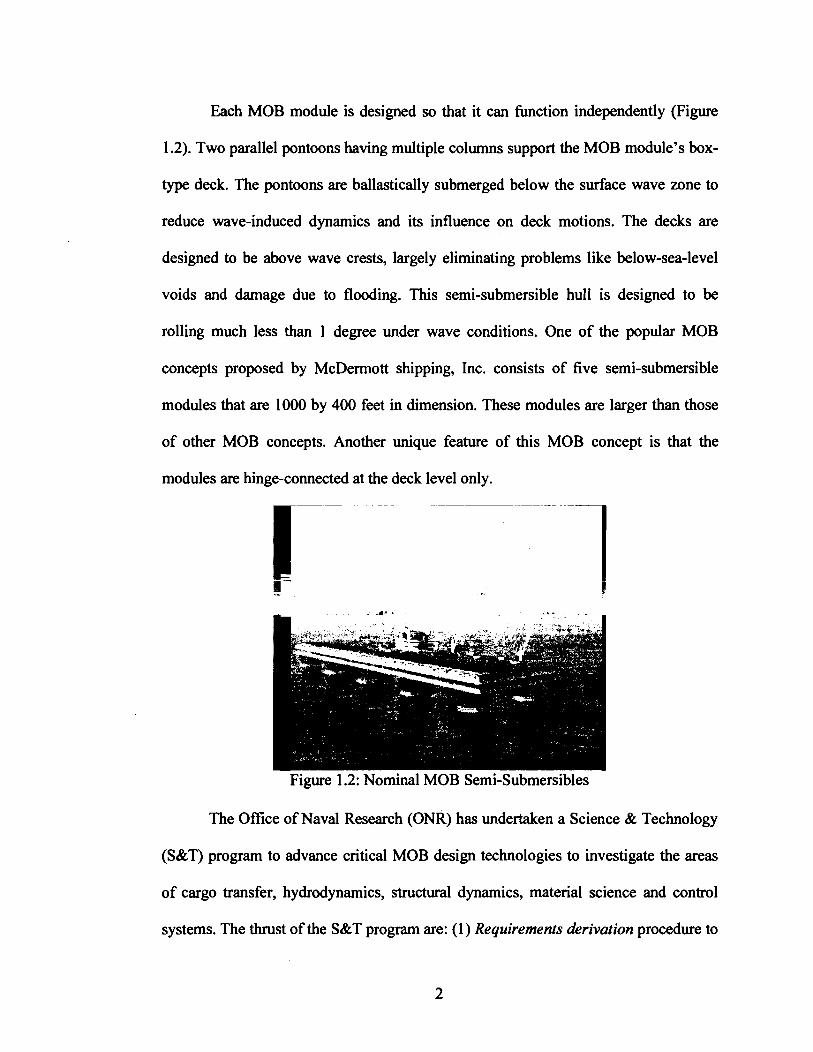
Each MOB module is designed so that it can function independently (Figure
1.2). Two parallel pontoons having multiple columns support the MOB module's box-
type deck. The pontoons are ballastically submerged below the surface wave zone to
reduce wave-induced dynamics and its influence on deck motions. The decks are
designed to be above wave crests, largely eliminating problems like below-sea-level
voids and damage due to flooding. This semi-submersible hull is designed to be
rolling much less than 1 degree under wave conditions. One of the popular MOB
concepts proposed by McDerrnott shipping, Inc. consists of five semi-submersible
modules that are 1000 by 400 feet in dimension. These modules are larger than those
of other MOB concepts. Another unique feature of this MOB concept is that the
modules are hinge-connected at the deck level only.
Figure 1.2: Nominal MOB Semi-Submersibles
The Office of Naval Research (ONR) has undertaken a Science & Technology
(S&T) program to advance critical MOB design technologies to investigate the areas
of cargo transfer, hydrodynamics, structural dynamics, material science and control
systems. The thrust of the S&T program are: (1) Requirements derivation procedure to

define the mission needs, (2) a set of performance tools to measure the cost and
performance of a MOB concept, (3) wave characterization on a large scale, (4) MOB
classiJcation guide to document performance and reliability, (5) hydrodynamic and
hydroelastic computer models for the analysis of critical MOB aspects like connector
loads, air gap limits between ocean and bottom of deck, transit behavior, stability and
extreme response, (6) control s o f ~ a r e to coordinate up to eight thrusters located on
each of the MOB modules, and (7) four unique, innovative MOB concept designs
distinguished by their method of connection. The technology developed through this
program can be extended to a host of commercial applications like Ocean Thermal
Conversion (OTEC), offshore industrial bases, and offshore aquaculture.
This thesis work aims at providing necessary validation data to satisfy the
objective of developing hydrodynamic and hydroelastic computer models for the
analysis of critical MOB aspects. It utilizes physical scale model testing data that is
provided and attempts to describe the response of the MOB in terms of frequency
mode shapes and investigates the nonlinear characteristics of the response.
1.1 Physical Scale Model Tests
The ONR has sponsored a physical scale model testing on a 1:60 scale model of a
notional Mobile Offshore Base (MOB) for conducting seakeeping and structural loads
tests. The objective of the test program is to provide data for the validation of
analytical hydro computer programs using the physical model as the prototype. The
models will be Froude scaled (Sikora, 1998), including the scaling of the space frames
for structural frequency for dynamic responses.

The tests have been conducted in the Maneuvering and Seakeeping (MASK) at
the Naval Surface Warfare Center, Carderock Division (NSWCCD) for the following
cases: (1) single module, (2) a pair of connected modules (two module), and (4) four
connected modules. Wave related headings include head seas, bow quartering seas and
beam seas. All tests are conducted at zero speed.
The current test program represents a study of a hydroelastically scaled model.
Prior data from the NSWCCD tests of a 1/59' scale model of McDermott MOB
concept (Smith, 1998) are models that were not structurally scaled. Furthermore, one
data set from a particular design does not built sufficient confidence for universal use
of those models extrapolated to any MOB platform concept. The unusual size and
mission requirements also demand thorough validation of the tools that will be used
for design.
The primary objectives of this series of tests are: (1) to provide "generic"
validation data for the analytical hydro models/codes, (2) provide an accurate,
traceable database of module and module-to-module connector wave induced loads in
the linear and nonlinear response regimes for the validation of analytical codes, (3)
wave induced loads are defined as longitudinal, vertical and lateral bending moments,
vertical and lateral shear forces, and torsion caused by weight minus buoyancy loads,
(4) focus on the global response and loads of the hull girder and connectors rather than
local plate or shell loads and response, and (5) collect data in both the linear and
nonlinear regimes to provide a full validation of the hydro codes.

1.2 Objective
The objectives of this thesis are to study, analyze, and interpret the experimental data
available fiom the hydroelastic test model conducted at MASK as discussed in section
1.1. The goals of this effort can be summarized as follows:
Develop data reduction and analysis procedures to interpret the hydroelastic
test data.
Perform dynamic parameter estimation to obtain the modal fiequency of the
MOB models.
Investigate nonlinear dynamic characteristics using MIS0 direct and reverse
modeling.
The above procedure is achieved through the following steps: (1) Reduce and
process the experimental data, and (2) perform linear and nonlinear analysis of data
using the wave motion response as the primary input and the module motion response
(heave, pitch, roll, etc.) as the primary output response to generate a frequency
response function (FRF) and their statistical parameters, and (3) animate the response
of the MOB scale model and determine the mode shapes.
For data reduction and processing, a program Dynamic Data has been
developed based on Delphi to read the experiment data files and perform a data
reduction. The same program is also used to average the Z acceleration data channels
to obtain the heave acceleration response in the absence of a heave sensor. The
Dynamic Data program is also used to perform a linear Single-InputJSingle-Output

(SYSO) analysis of the data and generate corresponding FRF, coherence and phase
plots.
To perform a nonlinear analysis, the reduced data is processed using the ITAP
2000 data processing package on MATLABTM, to perform a Multiple-InputfSingle-
Output (MYSO) analysis to generate the FRF, coherence and phase plots. This
involves developing differentiation and integration schemes to obtain the motion or
velocity from the accelerations or the displacements.
To visualize the response of the MOB scale model, a program MOB-Animate
has been developed based on Delphi to read the frequency domain X, Y and Z
acceleration data and their phases and perform an animation of the response at
different frequency values. This program can depict a combination of modes that
occur at any particular frequency.
1.3 Scope of Work
The theoretical background of fluid-structure, wave theory, and wave spectrums is
discussed in Chapter Two of this thesis. Chapter Three discusses the physical scale
model and the data reduction, differentiation and integration techniques. Chapter Four
discusses the analysis techniques including FRFs, coherence and phase, SYSO and
MYSO. Chapter Five summarizes the analysis results for a single scale module for two
different waves spectrums. Chapter Six summarizes the analysis results for a two and
four module scale model. Discussion of summary, conclusions and future work is
carried out in Chapter Seven.

Chapter 2
Fluid-Structure Interaction and Wave Theory
An elementary understanding of fluid-structure interaction theory is an essential
component of understanding the dynamics of the MOB scale model. The theory is
introduced with fundamentals and the non-dimensional parameters analyzed herein
specifically associated with fluid-structure interaction theory. It is then developed by
discussing vortex-induced vibration, both in laminar and turbulent situations and a
brief examination of a ship motion in a seaway. The concept of "added mass" effect is
briefly examined. The discussion is concluded with a brief overview of waves and
wave spectrum. The latter is due to our interest in analyzing large oceanic floating
platforms.
2.1 Fundamentals
Fluid structure interaction is dynamic in nature and depends on several factors. The
most important of those factors are summarized below:
Position of structure relative to the fluid flow.
Velocity of the motion of the structure relative to the fluid flow.
Turbulence generators (time dependent) in the upstream fluid flow.
Characteristics of the fluid flow.
Structures can be optimized for efficiency in fluid conditions or be "bluff
structures" - structures in which the flow separates from a large section of the

structural surface. These structures are not optimized for hydrodynamic efficiency. All
are expected to withstand fluid forces. Most fluid flow equations contain nonlinearities
(e.g. nonlinear deformation of structure with increasing load) and nonlinear
extrapolations of the measurements of lift, drag or surface pressure are used in solving
equations. However, a few general solutions do exist utilizing sets of non-dimensional
parameters that can be usefil in obtaining solutions for a wide variety of problems.
For more complex models, however, the use of a research-quality numerical analysis
program becomes quite indispensable. Non-dimensional parameters of a two-
dimensional, spring-supported, damped structural model exposed to a steady flow are
given in appendix A.
2.2 Fluid-Structure Interaction - Basic Vortex Theory
The shear layers bounding the structure create vortices in the fluid flow past the
structure. This vortex creates a structural vibration called vortex-induced vibration.
These vibrations of can be of large amplitude. The nature of the vibrations depends
largely upon the Reynolds numbers of the fluid flow. Much of the vortex theory is
developed for circular cylinders and hence most of the theory discussed pertains
specifically to circular cylinders. Approximations for other shapes can however be
made by finding their circular equivalent.
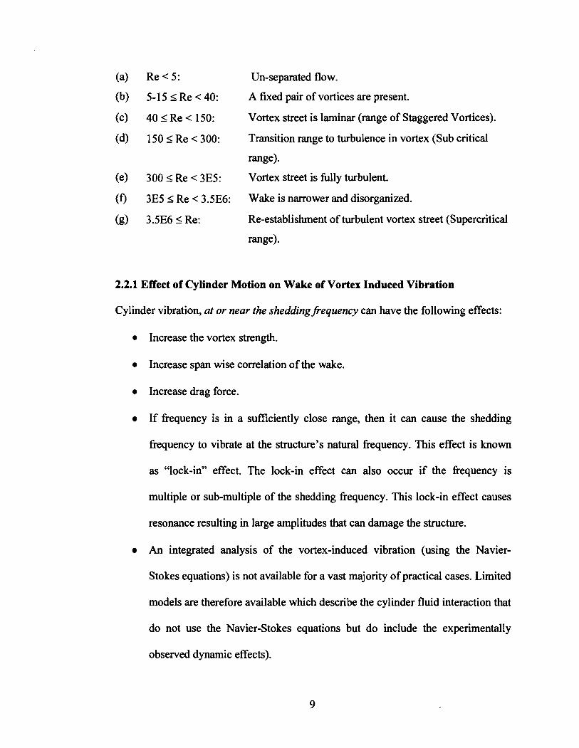
For a smooth, circular cylinder in subsonic flow, the period of the oscillation is
a bc t ion of Reynolds number. Based on the Reynolds number, the vortex can be
described as follows:
300 _< Re < 3E5:
3E5 I Re < 3.5E6:
3.5E6 I Re:
Un-separated flow.
A fixed pair of vortices are present.
Vortex street is laminar (range of Staggered Vortices).
Transition range to turbulence in vortex (Sub critical
range).
Vortex street is hlly turbulent.
Wake is narrower and disorganized.
Re-establishment of turbulent vortex street (Supercritical
range).
2.2.1 Effect of Cylinder Motion on Wake of Vortex Induced Vibration
Cylinder vibration, at or near the sheddingfiequency can have the following effects:
Increase the vortex strength.
Increase span wise correlation of the wake.
Increase drag force.
If frequency is in a sufficiently close range, then it can cause the shedding
frequency to vibrate at the structure's natural frequency. This effect is known
as "lock-in" effect. The lock-in effect can also occur if the frequency is
multiple or sub-multiple of the shedding frequency. This lock-in effect causes
resonance resulting in large amplitudes that can damage the structure.
An integrated analysis of the vortex-induced vibration (using the Navier-
Stokes equations) is not available for a vast majority of practical cases. Limited
models are therefore available which describe the cylinder fluid interaction that
do not use the Navier-Stokes equations but do include the experimentally
observed dynamic effects).

2.2.2 Vortex Induced Oscillations - Models
Two important models have been developed to describe the vortex induced
oscillations. These are:
Wake Oscillator Model (cylindrical structures only).
Correlation model (right circular cylinder).
2.2.2.1 Wake Oscillator Model (Cylindrical Structures Only)
This model is valid in the Reynolds number range lo3 - lo5 of a 2-D flow. It makes
the assumptions that the flow field outside the near wake is inviscid and that well-
formed vortex sheet and shedding frequency is present. The vortex is formed only in
the boundary layer (BL) and grows uniformly to a maximum strength and moves
downstream. Fluid force on cylinder is dependent on average fluid velocity and
acceleration.
The natural frequency of the shedding frequency is given by the equation
(Blevins, 1977)
u As 2 ( u, - translational velocity of the vortex street, U- free stream velocity,
U
D - cylinder diameter, K ' - proportionality constant)is a constant for a large range of
Re numbers, w is proportional to the ratio of the free stream velocity to the cylinder
diameter. This model predicts that the elastically mounted cylinder will exhibit large
amplitudes of oscillation as the vortex shedding frequency approaches the natural

cylinder frequency. The frequency of the vortex shedding is entrained by the natural
frequency of the structural oscillation and this effect is called "entrainment effect".
The peak resonant cylinder amplitude can be expressed in terms of reduced damping,
6, (Blevins, 1977)
where m = mass of structure 4 = damping factor p = density of structure material D = diameter of cylinder
As damping reduces, the peak resonant amplitude increases until maximum limiting
amplitude is reached. The amplitude ratio for 2E2 < Re < 2E5 is given by (Blevins,
where Ay is the vibration amplitude, 6, is reduced damping, S is the Strouhal
' A list of mode shapes, natural Erequencies and geometric factors for different types of cylindrical objects are provided in Table 3-2, pg. 32 of "flow-induced vibration" by Robert D.Blevins. See bibliography.
11

0 shape ry and equivalent mass term . The motion of the cylinder can be
lv4 (4dz 0
given by y = A, v(z) cos wst .
2.2.2.2 Correlation Model (Right Circular Cylinder)
The correlation model is based on span wise correlation and the cylinder amplitude
dependence on the vortex forces, which are absent in the wake oscillator model. This
model is valid in the Re range of 2E2 < Re < 2E5 and is limited to the resonance of a
single mode of vortex shedding. At resonance, the amplitude of the correlated life
force on the cylinder can be represented as a continuous function of cylinder
amplitude and a characteristic correlation length can represent spanwise correlation of
the fluid force.
The amplitude ratio obtained by this model is given by (Blevins, 1977)
where, CLE = 0 L , is the uniform lift coefficient per unit length and CL(z)
J v w z 0
is the lift coefficient. The motion of the cylinder can be given by
A Y Y(z,t) = Ayy/(z)coswst. The amplitude ratio - is a function of the damping D

L 2m(21r5) ( 2 ~ 9 , and fineness ratio -. At resonant vibration amplitudes of 0.1 pD2 D
diameter or smaller, the spanwise correlation has a strong effect on cylinder response
as follows:
The equivalent force per unit length decreases as aspect ratio increases.
The correlated vortex forces increase with amplitude.
At resonant vibration amplitudes of 1 or smaller, the vortex forces tend to
decrease to zero with increasing amplitude.
This model is better than the wake oscillator model for prediction of vortex-
induced vibrations at low amplitudes.
2.2.3 Reduction of Vortex-Induced Vibration
Vortex induced vibrations need to be reduced to minimize possible damage to the
oscillating structure. This can be achieved in the following ways:
Using composite materials such as fiber reinforced plastic (FRP) instead of
welded steel.
Using materials of high internal damping.
Using external dampers.
Using devices to dissipate energy.
Avoiding resonance by keeping the reduced velocity below 1. This is achieved
in small structures by increasing the natural frequency through the
modification of the structure.

Change cross section - vortex shedding is eliminated or minimized in a
streamlined profile, which reduce side forces.
2.3 Basic Structural Vibration
For this report, only topics related to the following criteria will be discussed:
Free vibration.
Linear vibration.
Single or two degree of freedom (DOF) vibration.
Viscous damping.
23.1 Basic Vibration Definitions
2.3.1.1 Spring Stiffness
The spring stiffness is determined by the amount displacement that occurs in a spring
when subjected to a certain force according to the linear relation
Where K - spring stiffness F - the force the spring is subjected to. A - the displacement the spring undergoes when
subjected to the force F
2.3.1.2 Natural Frequency of Vibration
The natural frequency of vibration of a single degree of freedom structure is given by
the following formula
02 = K/M; f = oI(2n) Eq(2.6)

Where o - natural frequency K - spring stiffness M - the effective mass of the structure including
any added mass f - the natural frequency in Hz
In a complex structure, there can be several natural frequencies with corresponding
mode shapes. The primary frequency is referred to as the 1" or fimdamental mode, the
secondary as 2"d mode and so on. One of the techniques of FEA model validation is to
match the actual mode shapes of the physical structure (obtained through
experimentation) and compare it with those obtained through numerical analysis.
2.3.2 Vibrational Damping
In the physical realm, all free vibration comes to a stop over a period of time. One
reason for this is because the fluid (air, water, etc.) surrounding the vibrating structure
dampens the vibration until the vibration stops. Damping is higher, typically, with
denser surrounding fluid. Structures vibrating in water therefore are subjected to
greater damping when compared to that in air. There are 3 major types of damping:
Viscous damping - Damping due to surrounding fluid or "viscous like".
Coulomb damping - Damping due to dry or Coulomb friction.
Hysteretic damping - Damping caused by friction between internal layers,
which slip or slide when the structure deforms.
For practical purposes the damping offered by air is considered negligible. In
such cases where the surrounding fluid offers negligible damping, the structures damp

out due to material damping (internal) which is viscous like in nature. Only viscous
damping is discussed in this report, which is the case with most fluid-structure
interaction scenarios.
Viscous damping occurs when the surrounding fluid or material (internal)
offers damping. The basic equation of motion for the free vibration of the structure
subjected to viscous damping is (Rao, 1995)
where m - mass of vibrating structure x - displacement c - damping constant k - spring constant
The resultant frequency of the vibrating structure due to viscous damping is different
from the natural frequency of the vibrating structure and is given by (Rao, 1995)
where COD - damped frequency ( rdsec) CON - natural frequency ( rdsec) t;=c/cc - damping factor CC - critical damping constant
The value of t; determines the type of damped case
0 I t; < 1 - Under-damped case
t; = 1 - Critically damped case
t; > 1 - Over-damped case
The under-damped and critically damped cases are more frequently encountered. The
solution of Eq(2.7) for the under-damped case is given by (Rao, 1995)

The equation of motion for the critically damped case is given by (Rao, 1995)
where CI - xo c2 - xo + ~ N X O
2.4 Added Mass Effect
The added mass effect is the phenomenon in which an oscillating mass immersed in
fluid experiences effects of an increased mass, mass moment of inertia and damping.
This 'virtual' increase in mass, mass moment of inertia or damping due to the effects
of the surrounding fluid is called the added mass, added mass moment of inertia or
added damping. This effect is pronounced when the surrounding fluid density is
comparable to that of the structure. Added mass effect is of three types:
Addedmass.
Added mass moment of inertia.
Added damping.
2.4.1 Added Mass or the Inertial Mass of the Entrained Fluid
Added mass is the inertial mass of the fluid entrained by the structure and increases
the effective mass of the structure for consideration in determining the frequency of
vibration. For certain symmetries2, increasing the mass of the structure can incorporate
Added-mass tables are available in "Structural Vibrations in a fluid", Chapter 14, see bibliography item no. 4
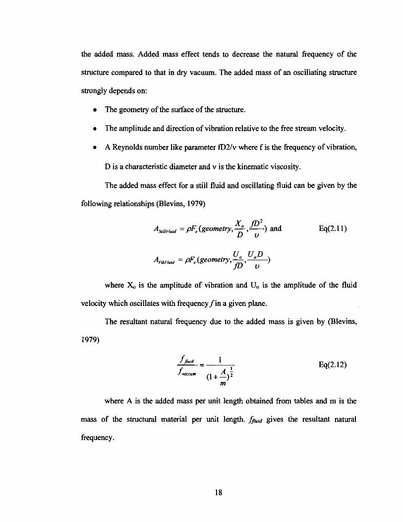
the added mass. Added mass effect tends to decrease the natural frequency of the
structure compared to that in dry vacuum. The added mass of an oscillating structure
strongly depends on:
The geometry of the surface of the structure.
The amplitude and direction of vibration relative to the free stream velocity.
A Reynolds number like parameter fD2Iv where f is the frequency of vibration,
D is a characteristic diameter and v is the kinematic viscosity.
The added mass effect for a still fluid and oscillating fluid can be given by the
following relationships (Blevins, 1979)
where X, is the amplitude of vibration and U, is the amplitude of the fluid
velocity which oscillates with frequency f in a given plane.
The resultant natural frequency due to the added mass is given by (Blevins,
1979)
f fluid 1
where A is the added mass per unit length obtained from tables and m is the
mass of the structural material per unit length. hUid gives the resultant natural
frequency.

2.4.2 Added Mass Moment of Inertia
Added mass moment of inertia of the fluid entrained by the structure as it rotates about
a fixed point. Similar to the added mass, the added mass moment of inertia increases
the effective mass moment of inertia of the vibrating structure. If the structure has
certain symmetries, the added mass moment of inertia can be incorporated directly in
the analysis to obtain the final response. In FEA models, the added mass moment of
inertia can be ignored if a sufficient number of elements are present. If the elements
are small, the mass moments of inertia of individual elements are negligible. The
added mass moment of inertia will be accounted for in a distributed manner. Added
mass moment of inertia tables are available (seefootnote 2).
2.4.3 Added Damping
Added damping is contributed by a damping forces that occurs due to water viscosity.
The damping force is assumed to be directly proportional to the relative speed between
the structure and the fluid for a linear response. The damping force can be expressed
by
0 0
where x is the speed of the structure, is the vertical component of the fluid
particle speed and b is the linear coefficient of friction. For a continuous structure
oscillating at its natural frequency in one mode in the y-direction, the equivalent
viscous damping coefficient for vibration in that direction is

where the numerator term is the energy expended in damping. The lower integral is
0
proportional to the maximum kinetic energy of the structure. [y(t)]L is the maximum
squared velocity achieved during one period (T) of vibration. Fd is the damping force
per unit length in Y direction, Y(z,t) = y(z)y(t) is the total displacement of the
structure in the y direction, m(z) is the mass per unit length of the structure including
the mass of entrained fluid, and z is the spanwise coordinate extending from z = 0 to z
2.5 Vibrations Induced by an Oscillating Flow
The in-line forces associated with the oscillating flow are the inertial force acting in
phase with the acceleration of the flow, and a drag force, which acts in phase with the
velocity ofthe flow. The solution of linearized equations of motion for in-line
motion is given by (Blevins, 1977)
where a, = (kxlm,,)ln - circular natural frequency in vacuum WN = (kxlm) In - circular natural frequency in fluid b - damping factor in vacuum <N - damping factor in fluid kx - effective spring constant CI - added mass coefficient A - cross-sectional area

- density of fluid - mass per unit length of structure - total mass per unit length (inc. added mass)
The total damping in the structure for an oscillatory flow with zero mean flow
is obtained using the following equation (Blevins, 1979)
where U, - mean fluid velocity CD - coefficient of discharge of fluid
To incorporate the effects of cross-sectional geometry, influence factors are added,
which are available in Table 6.1 in Chapter 6 of "Flow-induced vibration" (See
bibliography).
2.6 Ship Motion in a Seaway
2.6.1 Introduction
It is essential to predict the nature of sea waves and the response of a floating structure
to the sea waves to meet the following criteria:
The floating structure must not experience structural failure and should be
capable of working under damaged conditions.
The floating structure must not develop excessive motions to prevent the use of
critical machinery in heavy seas.

The floating structure must have acceptable levels of passenger and crew
comfort.
The primary difference between the analysis of a ship motion in a seaway to
that of flow-induced vibrations discussed above is in the treating of ship motions as
rigid body motions (ship deformations are negligible). The sea motion being non-
deterministic, is replaced within the limits of linearity and the response of the ship to a
complex sea can be found by summing the responses of a ship to a series of regular
waves. This analysis can be extended to other large floating platforms. Connected
platforms must consider the elasticity of the connector.
There are 3 translatory motions and 3 rotational motions associated with this
analysis:
3 Translatory motions:
qi = surge (in the direction of the headway)
qz = sway (horizontally perpendicular to the direction of the
headway)
q 3 = heave (translatory oscillation in the vertical direction)
3 Rotational motions:
q4 = roll (about the longitudinal axis)
qs = pitch (about the transverse axis)
T)6 = yaw (about the vertical axis)
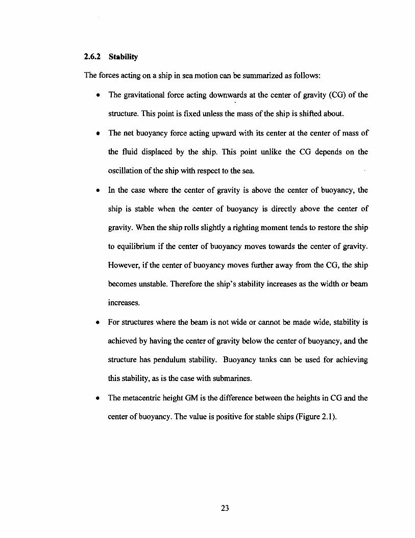
2.6.2 Stability
The forces acting on a ship in sea motion can be summarized as follows:
The gravitational force acting downwards at the center of gravity (CG) of the
structure. This point is fixed unless the mass of the ship is shifted about.
The net buoyancy force acting upward with its center at the center of mass of
the fluid displaced by the ship. This point unlike the CG depends on the
oscillation of the ship with respect to the sea.
In the case where the center of gravity is above the center of buoyancy, the
ship is stable when the center of buoyancy is directly above the center of
gravity. When the ship rolls slightly a righting moment tends to restore the ship
to equilibrium if the center of buoyancy moves towards the center of gravity.
However, if the center of buoyancy moves further away fiom the CG, the ship
becomes unstable. Therefore the ship's stability increases as the width or beam
increases.
For structures where the beam is not wide or cannot be made wide, stability is
achieved by having the center of gravity below the center of buoyancy, and the
structure has pendulum stability. Buoyancy tanks can be used for achieving
this stability, as is the case with submarines.
The metacentric height GM is the difference between the heights in CG and the
center of buoyancy. The value is positive for stable ships (Figure 2.1).

(a) ship at equilibrium (b) stable ship (moment tends to (c) unstable ship return ship to equilibrium) (moment tends
to increase roll) G - Center of gravity; B - Center of buoyancy
Figure 2.1: Stability of Ship in Roll
2.6.3 Natural Frequencies
The natural frequency of roll, pitch and heave are given by the following equations:
2.6.3.1 Natural Frequency of Roll
The natural roll of a ship in motion will have a frequency of o~ (radls) given by the
following relationship (Blevins, 1977)
where h - Roll frequency (Hz) P - Water density v d - Volume of water displaced by hull I44 - Polar mass moment of inertia for
rotation about longitudinal axis A44 - Polar mass moment of inertia of the
added mass of water entrained by the hull.
g - Acc. due to gravity GM - Metacentric height

The formula is simplified by noting that b4 is proportional to mass of ship
multiplied by the square of the beam.
c4 - Prop. Constant (0.35 - 0.4) GM - Metacentric height b - Beam of the ship
The average natural frequency of most ships is generally between 0.033Hz to
0.25Hz. The larger the ship, the lower the natural frequency of roll.
2.6.3.2 Natural Frequency of Pitch
The natural pitch of a ship in motion will have a frequency op (radls) given by the
following relation (Blevins, 1977)
where fp - Pitch frequency (Hz) P - Water density
I 5 5 - Polar mass moment of inertia for pitch of the ship
A s s - Polar mass moment of inertia of the added mass of water entrained by the hull as the hull pitches.
g - Acc. due to gravity
b(x) - Beam of the ship as a function of x. L - Length of the ship
The formula is simplified by noting that 155 + ASS is proportional to M L ~ , and
pg ix2b(x)d* is proportional to M~L' 1 d we get L
where fp - pitch frequency (Hz) c5 - prop. Constant (0.13)
g - acc. due to gravity d - depth of hull
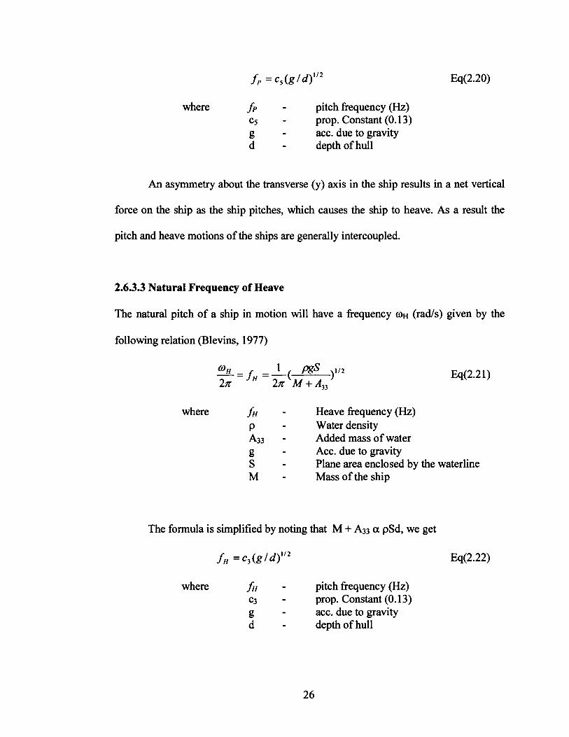
An asymmetry about the transverse (y) axis in the ship results in a net vertical
force on the ship as the ship pitches, which causes the ship to heave. As a result the
pitch and heave motions of the ships are generally intercoupled.
2.6.3.3 Natural Frequency of Heave
The natural pitch of a ship in motion will have a frequency o~ (radls) given by the
following relation (Blevins, 1977)
where f~ - Heave frequency (Hz) P - Water density
A33 - Added mass of water g - Acc. due to gravity S - Plane area enclosed by the waterline M - Mass of the ship
The formula is simplified by noting that M + Aa a pSd, we get
where f~ - pitch frequency (Hz) c3 - prop. Constant (0.13)
g - acc. due to gravity d - depth of hull
The pitch and heave are approximately the same for ships that are not
symmetric about the transverse axis (heaving also induces pitch).
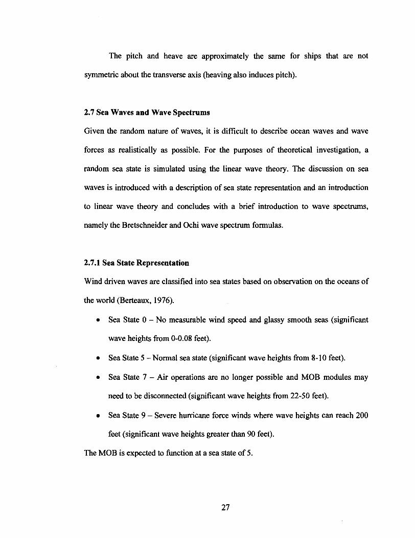
2.7 Sea Waves and Wave Spectrums
Given the random nature of waves, it is difficult to describe ocean waves and wave
forces as realistically as possible. For the purposes of theoretical investigation, a
random sea state is simulated using the linear wave theory. The discussion on sea
waves is introduced with a description of sea state representation and an introduction
to linear wave theory and concludes with a brief introduction to wave spectrums,
namely the Bretschneider and Ochi wave spectrum formulas.
2.7.1 Sea State Representation
Wind driven waves are classified into sea states based on observation on the oceans of
the world (Berteaux, 1976).
Sea State 0 - No measurable wind speed and glassy smooth seas (significant
wave heights from 0-0.08 feet).
Sea State 5 -Normal sea state (significant wave heights from 8-10 feet).
Sea State 7 - Air operations are no longer possible and MOB modules may
need to be disconnected (significant wave heights from 22-50 feet).
Sea State 9 - Severe hurricane force winds where wave heights can reach 200
feet (significant wave heights greater than 90 feet).
The MOB is expected to function at a sea state of 5.

2.7.2 Linear Wave Theory
The linear wave theory assumes that the fluid is incompressible, frictionless,
irrotational, and that the wave height is small in comparison to the wavelength and
ocean depth, d (Figure 2.2). The significant wave height is the average of the 113
highest waves and the significant wave period represents the period of maximum
energy content. At a sea state of 5, the significant wave height is 10 feet and
significant wave period is 6.9 sec.
Figure 2.2: Schematic Representation of a Simple Harmonic Wave
The linear wave theory is also known as the small amplitude wave theory. The
solution to the linear small amplitude wave theory can been summarized by the
following equations (Wilson, 1984):
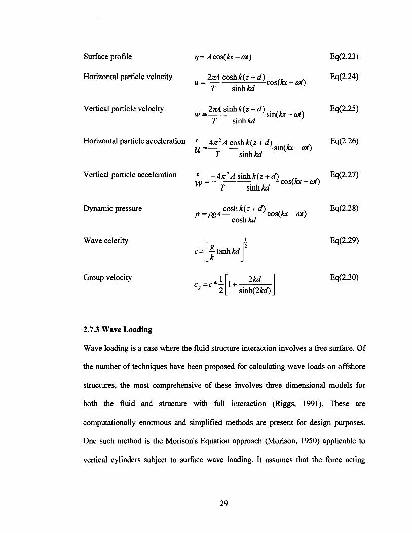
Surface profile q = A cos(kx - d ) Eq(2.23)
Horizontal particle velocity 2 d cash k(z + d) cos(h - ws) u =- Eq(2.24)
T sinhkd
Vertical particle velocity 2 d sinh k(z + d) sin(h - w =- Eq(2.25)
T sinhkd
Horizontal particle acceleration 0 4z2A cash k(z + d) sin(kr - Eq(2.26) U =T sinh kd
Vertical particle acceleration O -4z2Asinhk(z+d) cos(kx - ws)
Eq(2.27) w = T sinh kd
Dynamic pressure cosh k(z + d) Eq(2.28) * =pgA cosh kd
cos(kx - ws)
Wave celerity 1 Eq(2.29)
Group velocity
2.7.3 Wave Loading
Wave loading is a case where the fluid structure interaction involves a free surface. Of
the number of techniques have been proposed for calculating wave loads on offshore
structures, the most comprehensive of these involves three dimensional models for
both the fluid and structure with full interaction (Riggs, 1991). These are
computationally enormous and simplified methods are present for design purposes.
One such method is the Morison's Equation approach (Morison, 1950) applicable to
vertical cylinders subject to surface wave loading. It assumes that the force acting

transverse to the cylinder axis is made up of two components: a drag force, analogous
to the drag on a body subjected to steady flow of a real fluid associated with wake
formation behind the body; and an inertia force, analogous to that on a body subjected
to a uniformly accelerated flow of an ideal fluid. For a circular cylinder of diameter D,
Morison's Equation is expressed as
where F is force per unit length, u is fluid velocity, CD is a drag coefficient, C, is an
inertia coefficient, and r is the fluid density. The first term in this equation
corresponds to the drag force and the second term represents the inertia force. In
general the coefficients CD and C, vary with time and space with average values of
0.9 and 1.94 (Sarpkaya, 1981).
2.7.4 Wave Spectrums
For the scale model testing, the waves are generated using the Bretschneider and Ochi
formulas. The Bretschneider Double Height Spectra formula is an empirical spectral
density function with significant wave height, H,, significant wave period, Ts, arbitary
time period, T, and component wave height, S, as parameters (Berteaux, 1976) and is
given as
An example of the Bretschneider Double Height Spectra is shown below
(Figure 2.3 - see appendix B for MathCAD sheet)

Bretschneider Double Height Spectra
Figure 2.3: Bretschneider Double Height Spectra
Ochi and Hubble (1976) combined two sets of three-parameter spectra, one
representing low frequency components and the other the high frequency components
of the wave energy and derived the following Six-Parameter OCHI spectral
representation
An example of the OCHI Six-Parameter Spectra is shown below (Figure 2.4 -
see appendix B for MathCAD sheet)

OCHI Six-Parameter Spectrum
.s .oooox r o- 3. 0 J.~OOO.
Figure 2.4: OCHI Six-Parameter Spectrum
where j=1,2 stands for the lower and higher frequency components. The six
parameters Cl, &, o,l, hl, and h2 are determined numerically such that the
difference between theoretical and observed spectra is minimal and r is the Gamma
function.
2.7.5 Wave Conditions
Wave conditions can be primarily classified into small and large waves. Random seas
are further classified by three different unidirectional representations, namely, head
seas, beam seas and bow quartering seas (Figure 2.5).

(a) Hc ad St a
(c) Quadcrinp; Sea
Figure 2.5: Three Unidirectional Random Seas

Chapter 3
Physical Scale Model, Data Reduction, and Visualization Technique
3.1 Physical Scale Model
The design of the physical scale hydroelastic model (Figure 3.1) is based on the test
objectives, facility size and capability (Sikora, 1998). The test was based on the
assumption that the response of the structure affects the loads on the structure. Due to
conflicting non-dimensional requirements (e.g., Froude and Reynolds numbers), the
focus has been on using a structural scaling of the model. The elastic properties of the
scale model are designed such that the natural frequencies, flexibilities, and
displacements are within a range that could be expected of a hlly scaled MOB.
(a) Single Module Scale Model Test

(b) Four Module Scale Model Test
Figure 3.1 : Scale Models under Testing
3.1.1 Wave Tank
In designing the physical scale model, the following concerns are taken into account:
The largest possible physical scale model should be used for testing to
minimize model scale effects and maximize measurement signal to noise (S/N)
ratio. This would also minimize frictional force effects (Reynolds) as opposed
to inertial force effects (Froude).
The wave tank should be large enough to avoid blockage or wall effects at
head, following and oblique wave headings.
Wave makers must be able to generate good quality waves.
From the above it has been determined that the NSWCCD Maneuvering and
Seakeeping (MASK) Facility (Figure 3.2) meets all these requirements. The physical
characteristics of the MASK basin are 350 feet long by 240 feet wide. Based on using
the NSWC MASK, a model scale ratio of 60 was chosen for the MOB model. At this
model scale factor the total model length of a four module unit is just over 100 feet
long, which will avoid wall effects in the NSWC MASK facility.
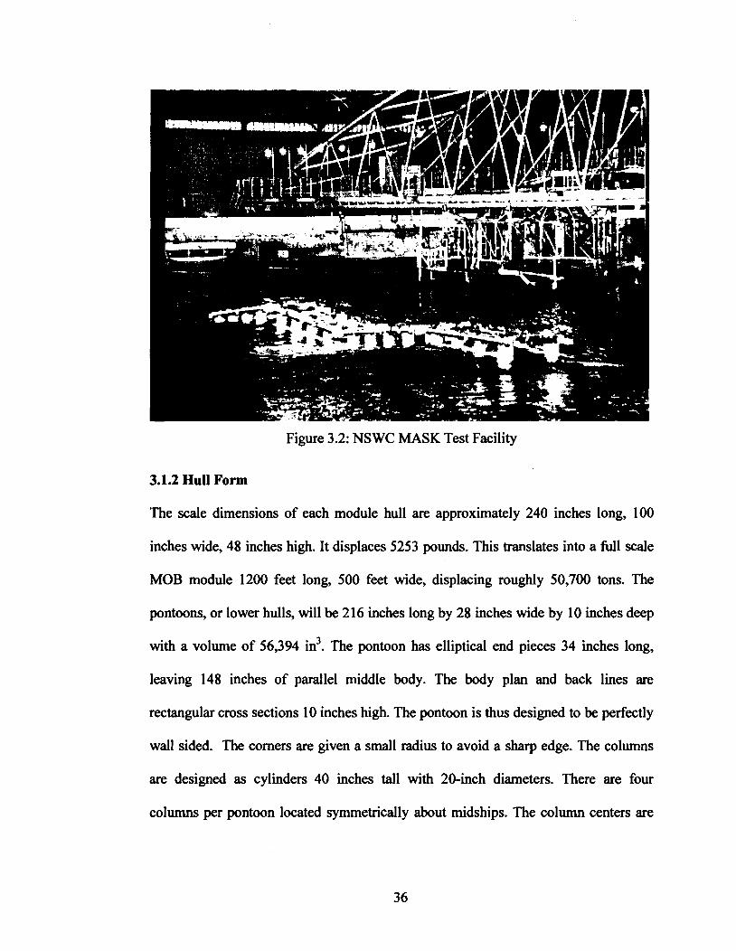
Figure 3.2: NSWC MASK Test Facility
3.1.2 Hull Form
The scale dimensions of each module hull are approximately 240 inches long, 100
inches wide, 48 inches high. It displaces 5253 pounds. This translates into a full scale
MOB module 1200 feet long, 500 feet wide, displacing roughly 50,700 tons. The
pontoons, or lower hulls, will be 216 inches long by 28 inches wide by 10 inches deep
with a volume of 56,394 in3. The pontoon has elliptical end pieces 34 inches long,
leaving 148 inches of parallel middle body. The body plan and back lines are
rectangular cross sections 10 inches high. The pontoon is thus designed to be perfectly
wall sided. The corners are given a small radius to avoid a sharp edge. The columns
are designed as cylinders 40 inches tall with 20-inch diameters. There are four
columns per pontoon located symmetrically about midships. The column centers are

27 and 81 inches fore and aft of midships. There is no special shaping where the
column meets the pontoon or upper box. The columns on each side are connected with
3 inch square PVC cross braces. These provide structural support for prying and
squeezing. The centers of the cross brace will be 14 inches above the baseline, or 4
inches above the top of the pontoon. Model structural segmentation is achieved by
attaching segments representing the hull attached to the continuous space fiame
connected by cross pieces. The pontoon will be made of four segments of equal
length each. Each segment has a column. The modules will not be self-powered nor
be remotely controlled. Bungee chords maintain the heading relative to the waves.
3.13 Internal Structure
NSWCCD has primarily considered three approaches for designing elastic models. In
the first approach, all the scantlings, decks, and bulkheads of the prototype are scaled
in a fully structural model. This will result in correctly scaled overall structural
properties. Small models, usually constructed with polyvinyl chloride (PVC) measure
the structural behavior as well as seaway loads of larger metal scales, the structural
members conforming to external geometry. The major disadvantage of such a model is
that it requires detailed prototype design and construction drawings, which is difficult
to achieve with a notional MOB scale model. This model is more applicable when
detailed MOB design has been established and can be used to evaluate the distribution
of the connector loads into the support structure in the box.
In the second approach, a flexible beam (backspline) model is used to measure
vertical bending, vertical shear, lateral bending, lateral shear, and torsion. This model
is appropriate for monohull ships that can be idealized as a simple beam in bending
and measures only loads. In reality, however, the load paths from the pontoons
through the columns into the box are three dimensional in nature and cannot be
modeled by a simple flexible beam. This is the major disadvantage of this model.
In the third approach, a three-dimensional space frame is designed to represent
the overall rigidity of each module to measure the responses of interest. The upper hull
consists of a structural ladder containing two rails that are aligned over the columns
and correspond to the primary load path from the end connectors. The rails of the
ladder provide the stiffness for vertical and lateral bending of the box while the
number, size and stiffness of the rungs determine the torsional properties. Vertical bars
attached to the rails of the ladder model the stiffness properties of the columns. The
stiffnesses of each of the lower hulls are also modeled by rails attached to the column
members. Structural foils connecting port and starboard columns complete the three-
dimensional space frame. Non-load bearing segments, corresponding to the external
geometry, are attached to the structural members. The major advantages of this model
are cost and the ability to model the structural properties, modal shapes and
frequencies.
Of the above three approaches, the third was selected due to its obvious
advantages. A notional MOB model with a conceptual ladder (Figure 3.3) was chosen
as the most appropriate structure for measuring seaway loads on the box. The
structural members are built up plastic (PVC) box beams, tubing or I-beams. Finite

element analyses of the designs were performed to confirm that all of the desired
stiffiesses were actually present. The complete model of each MOB module is
obtained by encasing the structural members with the lower hulls, columns, and upper
box composed of an appropriate shell material such as fiberglass, wood, or plastic.
(a) Structural Space Frame
(b) Lower Hulls and Columns Encasing Structural Members
Figure 3.3: MOB Structural Model

3.1.4 End Connectors
The connection of the modules to each other is achieved through a notional connector
(Figure 3.4). The connector represents a realistic stiffness for the axial loads that cause
vertical bending, lateral bending, and torsion in the modules. For these model tests,
multi-parameter load cells will be used to measure the connector forces.
(a) MOB connector attached to rail end (b) 34" MOB Model Connector
Figure 3.4: MOB Connector
3.1.5 Ballasting
In order to maintain the possible motion and period values of a full-scale model, each
module is ballasted using a combination of lead weight and floodable space. To float
at a 23-inch draft, the model displaces 5253 lbf. The model (structure and shell) and
data measurement system weigh approximately 2000 lbf. The lead weight (989 lbfs)
is used to adjust the draft up to 11 inches. The remaining 2255 lbfs of ballast is in
floodable ballast tanks in the pontoons. These tanks are completely flooded to avoid

any sloshing. Each tank has plugs on the top and bottom and sloping sides to ensure
complete flooding and drainage.
3.1.6 Instrumentation
The primary instrumentation on the model consists of load cells for measuring inter-
modular connector loads. The space frame is instrumented with strain gages for the
measurements of internal module loads and mode shapes. Pressure gauges and panel
sized pressure sensors are also installed to provide measurements of the hydrostatic
pressure fields and local wave impacts. The first order six degree of fieedom motions
are measured or calculated for each module by use of triaxial accelerometers (Figure
3.5). Connector responses were measured through a specially designed force
transducer. This device isolated the vertical, longitudinal and transverse forces and
moments using a set of four pins at each connector location. Video and photographic
documentation of the tests have been conducted. The far and near field wave
measurements will be used as the inputs and outputs for analysis.
I Bow
(a) Single Module

P o r t C o n n e c t o r <I I Bow
S t a r b o a r d C o n n e c t o r
(b) Two-Module
P o r t C o n n e c t o r
32 31 30 29 24 23 22 21 16 15 14 13 8 7 6 5 X
E::DT-::K- : : : L::: 28 27 26 2 5 20 19 18 17 12 11 10 9 4 3 2 1
S t a r b o a r d C o n n e c t o r
(c) Four-Module
Figure 3.5: Location of tri-axial accelerometers
3.2 Data Reduction
In order to perform a dynamic data analysis, a program, Integrated Test and Analysis
Processor (ITAPTM) distributed by Measurements Analysis Corp. was chosen which
runs as a subset of MATLABTM and is currently distributed by Measurements Analysis
Corp. Importing of large sets of data into MATLABTM is very time-consuming and
inefficient. Hence efficient data reduction techniques are required.
The MOB data sets were oversampled to allow for post test digital filtering.
Also, many more channels were recorded than are required to meet the objectives of
the current analysis. To alleviate the processing difficulties, an application program
called DynamicData (Figure 3.6) was written at the University of Maine in DELPHITM.

The purpose of this program is to read in the large MOB data set, reduce the data set to
a subset of selected channels, filter the data, decimate the data, compute the power
spectra, the FRF, the phase and the coherence based upon a selected reference
channel. It also allows channels to be averaged. This is particularly u se l l in
averaging the Z accelearations to obtain the heave acceleration response in the absence
of a heave sensor. It also provides a graphical visualization of the results. Multiple
records can be processed utilizing different windows and overlapping of records. This
program writes a reduced data set for faster processing with MATLABTM and
Figure 3.6: DynamicData Program

3.2.1 Differentiation and Integration Scheme
In order to perform analysis of the experimental data, the heave motion response is to
be extracted from the averaged Z acceleration measurements from the accelerometers
0
on the scale model. The velocity of the wave response w(t), w(t) is obtained using
the built in differentiation tools of MATLABTM. MATLABTM does not have built in
integration tools for integration based on random data vectors. In order to obtain the
heave motion, the average heave acceleration needs to be integrated twice. This
integration is achieved using the constant acceleration method.
The constant average acceleration method uses an initial velocity condition and
calculates the velocity based on the area under the curve (Figure 3.7) between two
points on the time history of the acceleration data.
Figure 3.7: Constant Acceleration Method of Integration
The change in velocity, Av, is given by the area of the curve given by the following
equation

The velocity is given by the following equation
The MATLABTM code for the above is given below (given an acceleration vector 'a'
of size 'm' with time step 'dt'):
v = zeros (m, 1) ; for i=l: (m-1)
dt = Time (i+l, 1) -Time (i, 1) ; da = a(i+l,l) - a(i,l); dv = a(i,l)*dt + 0.5*da*dt; v(i+l,l) = v(i, 1) + dv;
end
3.2.2 Noise Removal (Filtration)
Using the integration scheme discussed above, the acceleration time history profile
shown in Figure 3.8(a) yields the corresponding velocity time history profile shown in
Figure 3.8(b). It can be seen from the velocity profile, that the integration scheme has
introduced a low frequency noise that needs to be removed. Applying filters directly to
the time history velocity profile introduces changes to the amplitude and phase of the
integrated velocity profile. Hence noise removal is achieved in the frequency domain.
The Fast Fourier Transform (FFT) of the velocity obtained is shown in Figure 3.8(c)
and the low frequency noise is removed from the profile, shown in Figure 3.8(d). The
high pass frequency cut-off limit is determined through visual inspection of noise and
in this analysis is determined to be 0.1 Hz, i.e., all frequencies of 0.1 Hz or lower are
removed as being noise. The inverse of the filtered velocity FFT gives the required
time history profile of the velocity, shown in Figure 3.8(e). To obtain the displacement
time profile, the technique is repeated on the velocity time history data.

-0.04 1 20 40 90 00 100 120
TI- - -=Ma
(a) Acceleration Time History
(b) Integrated Acceleration (Velocity) Time History
(c) Frequency Spectrum of Velocity Time History

(d) Filtered Frequency Spectrum
(e) Inverse FFT - Filtered Velocity
Figure 3.8: Noise Filtration Technique
The above procedure is designed as a b c t i o n dsp - dzrfor differentiation and
alppint for integration (code listed in appendix C) with the following syntax
[y, v, a] = dsp-diff(a-t, s k q , FMax, Wn) [y, v, a] = dsp-int(a-t, sfreq, FMax, Wn)
where y, v, a = the displacement, velocity and acceleration a-t = input time history data for acceleration (a = at) sfreq = sampling frequency FMax = max frequency range Wn = high pass frequency value (freq < Wn = noise)

3.3 Visualization Technique
To get a better understanding of response of the MOB scale model, an animation
program called MOB-Animate was written at the University of Maine in DELPHITM
(Figure 3.9). This program reads one, two and four module data containing the X, Y
and Z acceleration data of all the sensors in the frequency domain along with the phase
information. It accounts for the time lag in response of sensors located at different
points along the MOB scale model and animates the response of the model at different
frequencies. This allows for better visual understanding of the MOB structure
response. The front, side, top and isometric views of the structure can be seen and the
response amplitude can be scaled. There are 8 triaxial accelerometers for each module
which are represented by black lines and the connectors are shown using red lines. The
connectors simply connect the ends of the modules and are not constrained in any
way.
Speed
. . --
I
Ampltude ' Frequency R;li( Response
R 3 Response
Figure 3.9: MOB-Animate Animation Program

To assess the vibration mode shape at a particular frequency the relative FRF
amplitude and phase information are used to reconstruct the shape based upon the
expression:
xi = Aisin(2xfit + +i) Eq(3.3)
At a particular frequency, the time parameter can be chosen to correlate to a particular
degree of phase shift. In doing so, the change in shape of a particular mode over one
period of oscillation can be ascertained.

Chapter 4
Frequency Response Functions, SllSO and MllSO Analysis
4.1 Frequency Response Functions
Frequency response functions (FRF) are used to describe the input-output (e.g., wave-
heave) relationship of a given system (Alleman, 1995). For experimental modal
analysis, the frequency response function is the most important measurement to be
made. For linear or nearly linear systems, the FRF is assumed to be linear. For
nonlinear systems, the measurement of the FRF may also be dependent upon the
independent variables. In this way, a conditional frequency response function is
measured as a function of the input amplitude and of the other independent variables
in addition to frequency. Before estimating the FRF the following important aspects
need to be remembered:
The dynamic properties of the system determines the frequency response
functions for given inputloutput parameters.
It is important to eliminate or minimize all errors (aliasing, leakage, noise,
calibration, etc.) when collecting data.
If all noise terms are identically zero, the assumption concerning the
source/location of the noise does not matter. Hence eliminating the source of
noise is important.
Modal parameters are only as accurate as the FRF they are estimated from.

FRF's can be based on four different configurations of input and outputs: (a)
Single inputlsingle output (SUSO), (b) Single inputlmultiple output (SUMO), (c)
Multiple inputlsingle output (MVSO), and (d) Multiple inputlmultiple output
(MUMO). The SUSO is used for time invariance problems between measurements.
The SUMO is applied in time invariance problems between measurements fiom
different inputs. The MVSO detects repeated roots and is used where there are more
than one input in a measurement cycle. The MUM0 is generally the best overall
testing scheme with consistent frequency and damping for all data acquired
simultaneously.
The estimation of the FRF is based on the transformation of data from the time
domain to the frequency domain. Computationally, a fast Fourier transform (FFT) is
used to convert a time history data into the frequency domain. The frequency response
function(s) satisfy the following single [Eq(4.1)] and multiple [Eq(4.2)] input
relationships where X is the input, F is the output and H is the FRF function
Single Input Relationship
XP* HPQ = FQ
Multiple Input Relationship

A sample FRF generated by the Dynamic Data program for a single input and
single output is shown (Figure 4.1). For a multiple input case, the FRF has two
values, component FRF value and cumulative FRF value.
(a) Frequency Composition of Input (Wave Input) Spectrum
(b) Frequency Composition of Output (Heave Output)
(c) FRF Function from Input to Output
Figure 4.1: Sample FRF for a SI/SO Function

4.1.1 Coherence Function
The scalar or ordinary coherence function is a frequency dependent function carrying
a real value between zero and one. The ordinary coherence function indicates the
degree of causality in a frequency response function. If the coherence is equal to one
at any specific frequency, the system is said to have perfect causality at that frequency.
In other words, the measured response power is caused totally by the measured input
power. A coherence value less than unity at any frequency indicates that the measured
response power is greater than that due the measured input. This could possibly be the
extraneous noise contributing to the output power or nonlinearity in the system. Low
coherence does not necessarily imply poor estimates of the frequency response
function, but suggests more averaging for reliable results. The ordinary coherence
function (for the system depicted by Eq(4.1) is computed as follows:
Cross Power Spectra
N,, is the number of averages used to minimize the random errors (variance),
F* is the complex conjugate of F(o) and X* is the complex conjugate of X(o). Using
the above, the ordinary coherence function is given by:
2 I G X F , 1 GXF, G F X , ~ COH, =y , = - - GFF, GXX, GFF, GXX,,
Eq(4.5)

In general, the coherence can be a measure of the degree of noise
contamination in a measurement. With more averaging, the coherence may contain
less variance, giving a better estimate of the noise energy in the measured signal if
there are no bias errors. The coherence function corresponding to the FRF shown
above (Figure 4.1) generated by the Dynamic Data program for a single input and
single output is shown (Figure 4.2)
Figure 4.2: Coherence Function for a SIISO FRF shown in Figure 4.1
Comparing the coherence fkction to the FRF, it can be observed that the
coherence function is high between the range of 0.4-1 Hz, and the FRF also shows a
significant response in the same fiequency band. Similarly, the coherence shows good
causality in the region between 1.75-2.25 Hz excluding 2 Hz, which is supported by
the FRF.
Two special cases of low coherence are particularly important. The first case of
low coherence is due to leakage error occurring in one or both of the input and output
measurements. This causes the coherence in the area of the peaks of the fiequency
response to be less than unity. This can be reduced by the use of weighting functions
or cyclic averaging. The second case occurs when a significant propagation time delay
occurs between the input and the output. If a propagation delay of length t is compared

to a sample function length of T, a low estimate of coherence will be estimated as a
function of the ratio t/T. This propagation delay causes a bias error in the frequency
response and should be removed prior to computation.
4.1.2 Phase
The phase of the FRF is the shift of a periodic signal (output) compared to a reference
(input) signal of the same
four-quadrant arc tangent
FRF.
frequency. It is obtained by computing the angle using the
of the division of the imaginary over the real values of the
imag (FRF) real(FRF)
The phase function corresponding to the FRF and coherence functions shown
above (Figures 4.1 and 4.2) is shown below (Figure 4.3).
Figure 4.3: Phase Function for a SVSO FRF
4.2 SYSO & MYSO Analysis
The dynamic response of a single module scale model can be best analyzed using the
SVSO technique for linear response characteristics and MVSO technique for nonlinear

characteristics. Tests with small waves are expected to yield linear results only and
tests with large waves are expected to yield both linear and nonlinear results. The main
objective of the analysis is to identify appropriate linear and nonlinear
integrodifferential equations of motion that can describe the scale model motions in
waves. The SVSO and MYSO analyses are performed using the direct and reverse
techniques. The MVSO direct and reverse techniques are carried out using two-
inputlsingle-output and three-inputlsingle-output models. The following important
conclusions were drawn up regarding SVSO and MVSO analysis (Bendat, 1998):
For SDOF linear systems, the SVSO linear method can correctly identify the
system frequency response functions.
For SDOF nonlinear systems, the Reverse MVSO Technique can correctly
identify the system frequency response functions.
For SDOF nonlinear systems, SVSO based optimum linear frequency response
function estimates can give erroneous results compared to Reverse MVSO
techniques.
Serious mistakes can occur when nonlinear effects are undetected between
SVSO and Reverse MVSO results.
In order to develop the theoretical basis for the response of the single module
scale model, its response can be characterized by a six degree of freedom motion
model shown below (Figure 4.4).

Wave force in x-direction -i t- Surge in x direction
Wave force in y-direction Sway in y direction
Wave force in z-direction Heave in z direction
Wave moment in x-direction Roll about x axis
Wave moment in y-direction -i "'"EM Pitch about y direction
Wave moment in z-direction -l Yaw about z direction
(a) Physical Input/Output Model
Sway
Surge
Pitch
(b) Sea Motion
Figure 4.4: Six-DOF Sea Motion

4.2.1 Linear SUSO Model
Three independent SVSO models corresponding to the heave motion, roll angular
rotation and the pitch angular rotation can be proposed. For small waves, a linear
relationship can be assumed between the wave amplitudes and the resulting motions
and rotations of the scale model
The heave differential equation of motion with constant damping and stiffness
coefficients is given by
where z(t) is the physical heave motion output, w(t) is the wave amplitude input, m is
the mass of the scale model, and a33, ~33, k33 are constants. Eq(4.7) can be extended to
cover frequency-dependent damping and stiffness coefficients by using the heave
linear integrodifferential equation of motion
( + a ) ( ) + c 3 ( t - d + k ( ( t ) (t - d = w ) Eq(4.8)
where c33(7) and k33(7) are weighting functions. Taking the Fourier transforms of both
sides of Eq(4.8) yields the simple mathematical formula
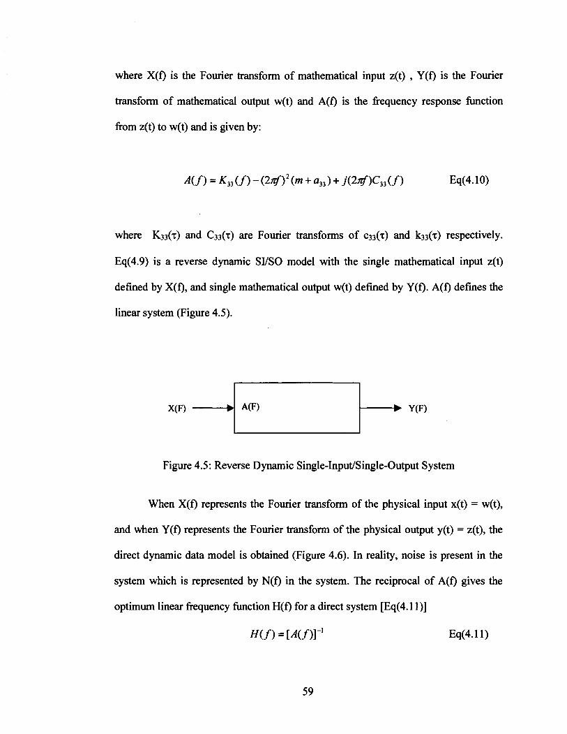
where X(f) is the Fourier transform of mathematical input z(t) , Y(f) is the Fourier
transform of mathematical output w(t) and A(f) is the frequency response function
from z(t) to w(t) and is given by:
where K33(~) and C33(r) are Fourier transforms of c33(r) and k33(~) respectively.
Eq(4.9) is a reverse dynamic SIISO model with the single mathematical input z(t)
defined by X(f), and single mathematical output w(t) defined by Y(f). A(f) defines the
linear system (Figure 4.5).
Figure 4.5: Reverse Dynamic Single-InputJSingle-Output System
When X(f) represents the Fourier transform of the physical input x(t) = w(t),
and when Y(f) represents the Fourier transform of the physical output y(t) = z(t), the
direct dynamic data model is obtained (Figure 4.6). In reality, noise is present in the
system which is represented by N(f) in the system. The reciprocal of A(f) gives the
optimum linear frequency function H(f) for a direct system rEq(4.1 I)]
H ( f = [A(f )I-' Eq(4.11)

Figure 4.6: Direct Dynamic Single-Input/Single-Output Linear Model
Similarly the roll rotation differential equation of motion with constant
damping and stiffness coefficients is given in Eq 4.12. The roll angular moment k(t)
has been replaced by an appropriate linearly equivalent w(t).
The pitch rotation linear differential equation of motion with constant damping
and stiffness coefficients is given below. The pitch angular moment M(t) has been
replaced by an appropriate linearly equivalent w(t).
(m + a,,) e(t) + c,, O(t) + k, O(t) = w(t)
Eq(4.12) and Eq(4.13) can be extended to generate the model discussed by
Eq(4.8-11).

4.2.2 Nonlinear MYSO Model
Many MYSO models can be proposed out of which special models relating to heave,
roll and pitch motions occurring in head, beam and quartering seas are considered.
These models have one linear input term and one or two parallel nonlinear input terms,
where the first nonlinear term represents a nonlinear relative hydrodynamic damping
force and the second nonlinear term represents a nonlinear restoring force. Both,
Direct MYSO and Reverse MYSO techniques are proposed.
4.2.2.1 Direct MYSO Nonlinear Model
The direct MYSO two-inputlsingle-output nonlinear integrodifferential equation of
motion can be represented by
where Xl(f) is the Fourier transform of the first physical input, X2(f) is the Fourier
transform of second physical (nonlinear) input, Y(f) is the Fourier transform of
physical output, Hl(f) is the frequency response function from Xl(f) to Y(f), and H2(f)
is the frequency response function from X2(f) to Y(f). This model is pictured below
(Figure 4.8) with a noise term N(f) representing deviations from the ideal model.
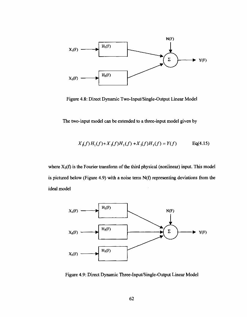
Figure 4.8: Direct Dynamic Two-Input/Single-Output Linear Model
The two-input model can be extended to a three-input model given by
where X3(f) is the Fourier transform of the third physical (nonlinear) input. This model
is pictured below (Figure 4.9) with a noise term N(f) representing deviations from the
ideal model
Figure 4.9: Direct Dynamic Three-Input/Single-Output Linear Model
62

The above two-input and three-inputlsingle-output models can be extended to
nonlinear models both in the time and frequency domain. In the time domain W and
0
W represent the wave motion w(t) and its derivative respectively. In the frequency
domain they represent the Fourier transforms of the wave motion w(t) and the Fourier
0
transform of its derivative respectively. Similarly, Z and Z represent the heave
motion z(t), P represents the pitch angle B(t) and R represents the roll angle #(t). The
first input Xl(f) is taken as the physical input from the wave w(t) and is given by
The second input term X2(f) is a physical input for a nonlinear relative hydrodynamic
damping force related to the relative velocity represented by:
x , ( f ) = ( 2 - i ) * I i-i I
For three-input models the third input model X3(f) is a physical input for a nonlinear
restoring force that varies for each case of interest. The output Y(f) is a physical
output that varies for each case. For given input and output records, the cumulative
coherence function and the associated values of the frequency response functions
Hl(f), and H2(f) in the two-input models and Hl(f), H2(f), and H3(f) in the three-input
models should be computed. The following two-input and three-input direct models
are proposed for the direct MYSO analysis:

Model D 1 : Heave Motions in Head Seas Using Large Wave Data
Direct Two-Input Model Direct Three-Input Model
x 1 W w
I i-i
Model D2: Pitch Motions in Head Seas Using Large Wave Data
Direct Two-Input Model Direct Three-Input Model
XI W W
Model D3: Heave Motions in Beam Seas Using Large Wave Data
Direct Two-Input Model Direct Three-Input Model

Model D4: Roll Motions in Beam Seas Using Large Wave Data
Direct Two-Input Model Direct Three-Input Model
x1 W W
Model D5: Heave Motions in Quartering Seas Using Large Wave Data
Direct Two-Input Model
XI w
Model D6: Roll Motions in Quartering Seas Using Large Wave Data
Direct Two-Input Model
XI w
Model D7: Pitch Motions in Quartering Seas Using Large Wave Data
Direct Two-Input Model
4.2.2.2 Reverse MIISO Nonlinear Model
The reverse MUSO two-inputfsingle-output nonlinear integrodifferential equation of
motion can be represented by:
where Xl(f) is the Fourier transform of the first mathematical input, X2(f) is the
Fourier transform of second mathematical (nonlinear) input, Y(f) is the Fourier
transform of mathematical output, Al(f) is the frequency response function from Xl(f)
to Y(f), and A2(f) is the frequency response function from X2(f) to Y(f). This model is
pictured below (Figure 4.10) with a noise term N(f) representing deviations from the
ideal model

Figure 4.1 0: Reverse Dynamic Two-InpuVSingle-Output Linear Model
The two-input model can be extended to a three-input model given by
where X3(f) is the Fourier transform of the third mathematical (nonlinear) input. This
model is pictured below (Figure 4.1 1) with a noise term N(f) representing deviations
from the ideal models
Figure 4.1 1 : Reverse Dynamic Three-InpuVSingle-Output Linear Model

The above two-input and three-inputlsingle-output models can be extended to
nonlinear models both in the time and frequency domain. In the time domain W and
0
W represent the wave motion w(t) and its derivative respectively. In the frequency
domain they represent the Fourier transforms of the wave motion w(t) and the Fourier
0
transform of its derivative respectively. Similarly, Z and Z represent the heave
motion z(t), P represents the pitch angle 8(t) and R represents the roll angle @(t). The
first input Xl(f) is taken as the mathematical input that varies with each case of
interest. The second input term X2(f) is the same mathematical input for a nonlinear
relative hydrodynamic term given in Eq 4.17 represented by:
For three-input models the third input model X3(f) is a mathematical input for a
nonlinear restoring force that varies for each case of interest. The output Y(f) is a
mathematical output from the wave w(t) given by
For given input and output records, the cumulative coherence function and the
associated values of the frequency response functions Al(f), and A2(f) in the two-
input models and Al(f), A2(f), and A3(f) in the three-input models should be

computed. The following two-input and three-input direct models are proposed for the
reverse MIISO analysis:
Model R1: Heave Motions in Head Seas Using Large Wave Data
Direct Two-Input Model Direct Three-Input Model
x1 Z Z
Model R2: Pitch Motions in Head Seas Using Large Wave Data
Direct Two-Input Model Direct Three-Input Model
x1 P P
x2 0 0 0 0 0 0
(z- w)* 1 i-i I (2- w)* I z- w 1
x3 0 P*IPl
Y W W

Model R3: Heave Motions in Beam Seas Using Large Wave Data
Direct Two-Input Model Direct Three-Input Model
Model R4: Roll Motions in Beam Seas Using Large Wave Data
Direct Two-Input Model Direct Three-Input Model
Model R5: Heave Motions in Quartering Seas Using Large Wave Data
Direct Two-Input Model
Model R6: Roll Motions in Quartering Seas Using Large Wave Data
Direct Two-Input Model
Model R7: Pitch Motions in Quartering Seas Using Large Wave Data
Direct Two-Input Model
4.3 SUSO and MYSO Analysis using the ITAP MATLAB Toolbox
The ITAP toolbox (M.A.Corp., 2000) provides several tools to perform random data
processing. The version used runs on MATLAB version 5.3. Out of these, the
following tools are used in the SYSO and MIIS0 analysis:
prel - Generate a single channel time history snapshot
Syntax: prel (X,dt,NFFT,namfil ,namch);
A descriptive display of a single channel time history array, X, sampled over
uniform time increments dt, is generated. Four plots appear in the display,
namely, (1) a time-frequency spectrogram, (2) time history trace, (3)

autospectrum, (4) probability density. A window length, NFFT, is specified for
spectrogram and autospectrurn calculations. Alphanumeric names "namfil"
(the data file name) and "namch" (the channel name) are specified for display
labeling. This routine is used within the ITAP-T function module prelim.
sisogen - Perform SVSO analysis computations
Syntax: [frq,HYX,COH,GYY,GXX,GYX] =
sisogen(X,Y,dt,nwin,novl);
This ITAP-T function module performs SVSO computations for one specific
input time history channel (columns of the matrix, X) and one specific output
time history channel (columns vector, Y), where the data is sampled over
uniform time increments, dt. The FFT window length, nwin, and overlap
processing index, novl, are specified as input parameters. Output arrays
resulting from the MVSO analysis consist of a frequency vector, frq, FRF
array, HYX, and ordinary coherence array, COH. Additional output arrays
consist of the output autospectrum, GYY, input autospectra, GXX, and
output/input cross-spectra, GYX. This function module should only be used if
GYY, GXX, and/or GYX are desired. Otherwise, use mimogen. This module
performs computations using the MATLAB Signal Processing Toolbox
function spectrum.

misogen - Perform MYSO Computations
Syntax: [fiq,HYX,COH,GYY,GXX,GYX] =
misogen(X,Y,dt,nwin,novl,iout);
This ITAP-T function module performs MYSO computations for an arbitrary
number of input time history channels (columns of the matrix, X) and one
specific output time history channel (columns vector, Y), where the data is
sampled over uniform time increments, dt, The FFT window length, nwin, and
overlap processing index, novl, are specified as input parameters. The integer
parameter, iout, is used by a "waitbar" display to inform the user of
computation progress during MIIMO analyses. Output arrays resulting from
the MYSO analysis consist of a frequency vector, fiq, FRF array, HYX, and
ordinary or cumulative coherence array, COH. Additional output arrays consist
of the output autospectrum, GYY, input autospectra, GXX, and outputfinput
cross-spectra, GYX.
pwrspec - Calculate and display the autospectrum or power spectral density of
a single channel time history array
Syntax: [fieq,gxx,stx]=pwrspec(tdata,dt,NFFT,namfil,namch);
This ITAP-T function routine calculates the autospectrum or power spectral
density of a single channel time history array X, sampled over uniform time
increments, dt. The user specifies a desired window length "NFFT" for the
spectral calculation. Alphanumeric names "namfil" (the data file name) and
"namch" (the channel name) are specified for display labeling. The output

arrays, fieq, gxx and stx represent the frequency array, autospectrum, and
tstandard deviation, respectively.
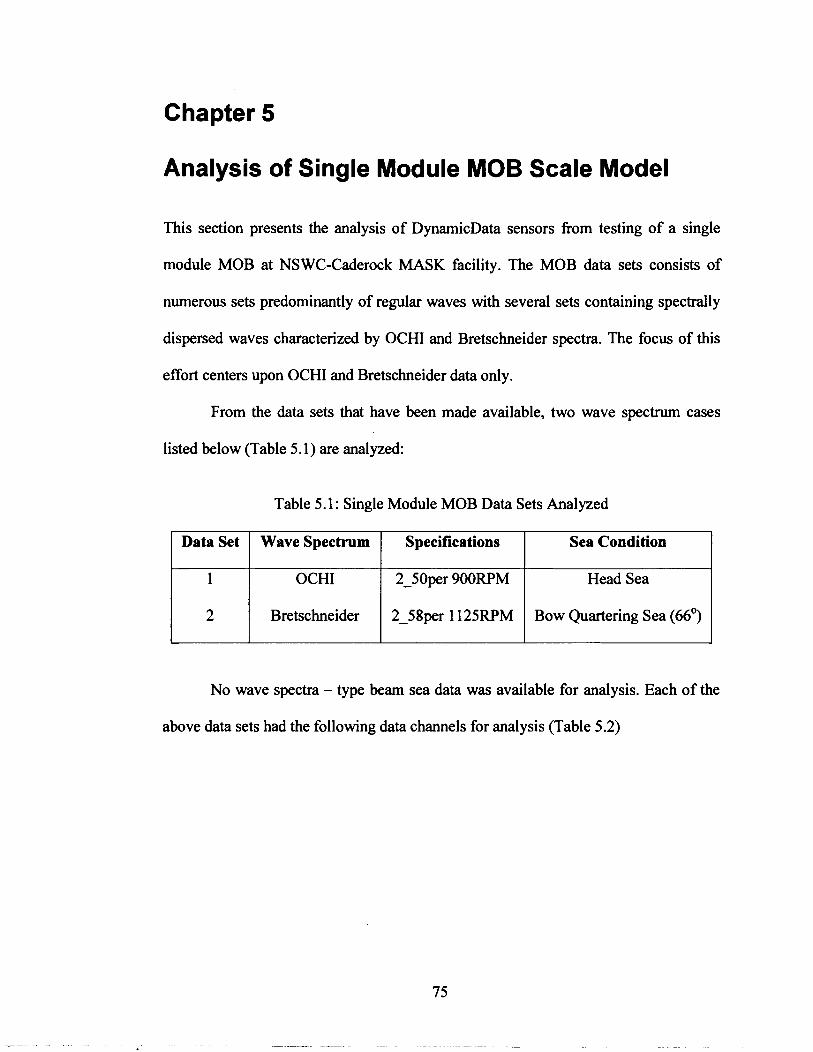
Chapter 5
Analysis of Single Module MOB Scale Model
This section presents the analysis of DynamicData sensors from testing of a single
module MOB at NSWC-Caderock MASK facility. The MOB data sets consists of
numerous sets predominantly of regular waves with several sets containing spectrally
dispersed waves characterized by OCHI and Bretschneider spectra. The focus of this
effort centers upon OCHI and Bretschneider data only.
From the data sets that have been made available, two wave spectrum cases
listed below (Table 5.1) are analyzed:
Table 5.1 : Single Module MOB Data Sets Analyzed
Data Set
k Wave Spectrum I Specifications I Sea Condition I
OCHI
No wave spectra - type beam sea data was available for analysis. Each of the
above data sets had the following data channels for analysis (Table 5.2)
Bretschneider
2-50per 900RPM Head Sea
2-58per 1 125RPM Bow Quartering Sea (66')
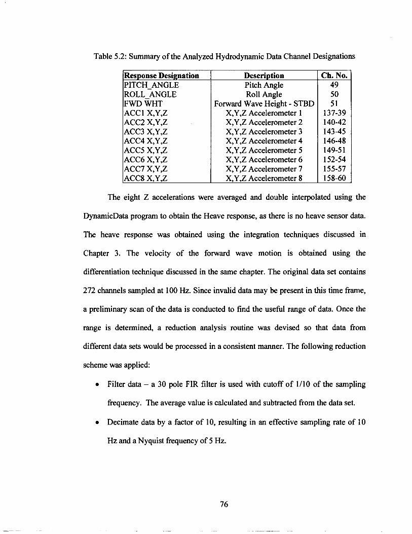
Table 5.2: Summary of the Analyzed Hydrodynamic Data Channel Designations
Res onse Desi nation 1- ROLL-ANGLE FWD WHT ACCl X,Y,Z ACC2 X,Y,Z ACC3 X,Y,Z ACC4 X,Y,Z ACCS X,Y,Z ACC6 X,Y,Z ACC7 X,Y,Z ACC8 X,Y,Z
Description Pitch Angle Roll Angle
Forward Wave Height - STBD X,Y,Z Accelerometer 1 X,Y,Z Accelerometer 2 X,Y,Z Accelerometer 3 X,Y,Z Accelerometer 4 X,Y,Z Accelerometer 5 X,Y,Z Accelerometer 6 X,Y,Z Accelerometer 7 X,Y,Z Accelerometer 8
Ch. No. 49 50 5 1
137-39 140-42 143-45 146-48 149-5 1 152-54 155-57 158-60
The eight Z accelerations were averaged and double interpolated usin the
DynamicData program to obtain the Heave response, as there is no heave sensor data.
The heave response was obtained using the integration techniques discussed in
Chapter 3. The velocity of the forward wave motion is obtained using the
differentiation technique discussed in the same chapter. The original data set contains
272 channels sampled at 100 Hz. Since invalid data may be present in this time frame,
a preliminary scan of the data is conducted to find the useful range of data. Once the
range is determined, a reduction analysis routine was devised so that data from
different data sets would be processed in a consistent manner. The following reduction
scheme was applied:
Filter data - a 30 pole FIR filter is used with cutoff of 1/10 of the sampling
frequency. The average value is calculated and subtracted from the data set.
Decimate data by a factor of 10, resulting in an effective sampling rate of 10
Hz and a Nyquist frequency of 5 Hz.

Compute the power spectral density (PSD) using a 256 point FFT, a Hanning
window, and an overlap of 50%. The final number of records depends on the
usefbl range of data determined.
Compute FRF - the frequency response functions were computed. Reference
channel selected was the wave height sensor FWD-WHT, a Hanning window,
and an overlap of 50%. The final number of records depends on the usehl
range of data determined.
During the data import process, the Z accelerations are averaged. The program
automatically performs a SUSO analysis on all the channels with respect to the
reference channel ( F W U H T ) . The reduced data is then exported to be further
processed by MATLABTM and EXCELTM.
5.1 SUSO Analysis - Comparison between DynamicData and ITAPM
A comparison of SUSO analysis between the DynamicData and ITAPT* analysis is
carried out to validate the analyses and also to study the differences in the two analysis
schemes. For this purpose a SUSO analysis is performed on Data Set 1 (see Table 5.1)
with the input as the FWD-WHT sensor and the output as the Average Z acceleration
which is the average of all the eight Z accelerometers for the module.

(a) Frequency Response Function
(b) Coherence Function
- ---
(c) Phase
Figure 5.1 : SI/SO Analysis using the DynamicData Program
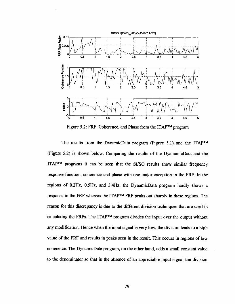
SVSO: I (FWDdT) QAVG Z ACC) b 001 H LL
LL
0.5 1 1.5 2 2 5 3 3 5 4 4 5 5
Figure 5.2: FRF, Coherence, and Phase from the ITAPTM program
The results from the DynamicData program (Figure 5.1) and the ITAPTM
(Figure 5.2) is shown below. Comparing the results of the DyanamicData and the
ITAPTM programs it can be seen that the SIISO results show similar frequency
response function, coherence and phase with one major exception in the FRF. In the
regions of 0.2Hz, OSHz, and 3.4Hz, the DynamicData program hardly shows a
response in the FRF whereas the ITAPTM FRF peaks out sharply in these regions. The
reason for this discrepancy is due to the different division techniques that are used in
calculating the FRFs. The ITAPTM program divides the input over the output without
any modification. Hence when the input signal is very low, the division leads to a high
value of the FRF and results in peaks seen in the result. This occurs in regions of low
coherence. The DynamicData program, on the other hand, adds a small constant value
to the denominator so that in the absence of an appreciable input signal the division

does not lead to a large spike. This prevents the FRF plot from being cluttered with
spikes in regions where the output signal is negligible.
5.2 Results of Analysis of a Single Module MOB Scale Model
The motion response of the single module data is first studied using the
MOB-Animate animation program. The significant frequencies of the six DOF system
is first visually determined. Then SUSO and MUSO techniques with appropriate
MUSO models, discussed in Chapter 4, are applied to the two data sets using the
ITAPTM. Table 5.3 lists the MUSO models that were applied to each of the data sets.
Table 5.3: MUSO Models Applied to the Data Sets
Data Set
1 I Bretschneider I Quartering I D5,D6,D7 I R5,R6,R7
1
Preliminary analysis of the wave data consists of time history plots, plots from
the MOB-Animate program, probability density function plots, and autospectral
density function plots. SUSO and MIISO analyses results are presented in terms of the
frequency response functions, coherence functions and phases. For the SUSO and the
MUSO analyses results, the frequencies extracted are for the peaks where the
corresponding coherence function is greater than or equal to 0.75. At these
frequencies, the random errors in estimating associated frequency response functions
Wave
Spectrum
OCHI
Sea Type Nonlinear Models applied
R1 ,R2 Head
Direct
Dl,D2
Reverse

are not as low. The initial points in the data set are ignored to exclude data
corresponding to the rampup section in the time history, where waves are allowed to
build up in amplitude.
5.2.1 Results for OCHI Head Sea 2-50per 900 RPM Data Set
The time history of the wave input and its frequency response is shown (Figure 5.3). It
can be seen from the time history that the input power is in the region of 0.45Hz to
2Hz with peaks at 0.625 and 0.781Hz. There is no significant input power below or
beyond this range.
(a) OCHI Wave Time History
Specln.m
- - - - -- A
(b) OCHI Wave Frequency Response
Figures 5.3: OCHI Wave for Single Module Test

Using the MOB-Animate program, the response of the OCHI Head Sea data
set is studied visually and the results are tabulated in Table 5.4 (Figure 5.5). These
observations are based upon visual inspection of the acceleration data simultaneously.
The corresponding coherence of the accelerations is shown in Figure 5.4.
Accelerations - Coherence
-- -
Figure 5.4: Coherence of Averaged X, Y and Z Accelerations for OCHI Single Module Data Set

Frequency (Hz)
0.09749 0.15599
0.23399
0.25349
0.29 - 0.60
Fable 5.4: Summary of Results for the OCHI Single Module
I Significant I Faint I Res~onse Res~onse
Period (seconds)
Response
4.27 1 Pitch and I * I
10.25 6.41
Surge Sway, Surge
3.95
Heave and
Pitch and
Roll Roll,
Heave
3.45 - 1.67
Rigid response
region (mild)
Sway Heave and
Coherence
0 - 0.27 (Poor)
* Sway
Heave and * Elastic response region Rigid
response region
0.78125 1 Heave and I
0.25 - 0.95
(good) 0.6 - 0.95
(good)
1.38 -
It can be seen from Table 5.4 that sway and heave are the significant motions
of the OCHI MOB single module model. As the orientation is head seas, there is poor
roll response of the structure and absent yaw response. There is no significant
response above 1.29 Hz. The structure shows elasticity in the 0.29-0.6 Hz and 0.8-1.28
Hz regions. This elastic behavior cannot be concluded as being that of the MOB
model. It could also be due to the local elasticity of the plate or layer on which the
accelerometers are mounted. As the MOB is designed to be elastic, it is desirable to
avoid the MOB hctioning in these ranges, specifically in the latter range. Surge and
sway dominate the initial rigid response region at 0.09749 Hz and 0.15599 Hz
Sway Pitch,
0.78
*
Sway No resmnse
(pronounced) Highly Elastic
*
0.3 - 0.95
No resDonse

respectively, while heave and pitch have pronounced mode shapes at 0.64349 Hz and
0.70 1 99 Hz respectively.
(a) Surge (0.09749 Hz) (b) Surge and Sway (0.1 5599 Hz)
(c) Pitch and Sway (0.23399 and 0.70199 Hz)

(d) Heave and Sway (0.25349 and 0.64349 Hz)
(e) Elastic Heave and Sway - first bending mode (0.29 - 0.60 Hz)
Figure 5.5: Mode Shapes of the Single Module OCHI MOB
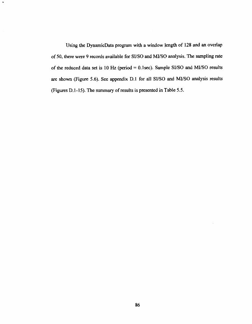
Using the DynamicData program with a window length of 128 and an overlap
of 50, there were 9 records available for SVSO and MVSO analysis. The sampling rate
of the reduced data set is 10 Hz (period = 0.1 sec). Sample SVSO and MVSO results
are shown (Figure 5.6). See appendix D.l for all SIISO and MVSO analysis results
(Figures D. 1 - 15). The summary of results is presented in Table 5.5.

Table 5.5: SVSO and MVSO Results for the OCHI Single Module MOB
Model I Response I Single Module Response I Other significant 1
FWD WHT z
I Range
. . SlSO W Z SlSO W P SlSO W R
(x i = zj i R l 2-Input:
-
- Max Freq., I Period, P
0.000 - 5.000 0.625
represents the peaks corresponding to maximum coherence where le; period is the inverse of the maximum frequency value
~re~uencies (Hz)
(Xi = P; X3 = P) 1 R2 3-Input: (X1 = P; X3= P) 2
* Max frequenc applicr

WSO: (FWD WHT), O(*AVG Z 1-8) I I I I I
-
I 1 I I I
2.5 3 3.5 4 4.5 5
(a) Sample SUSO Result - Input (FWD-WHT) and Output (Heave)
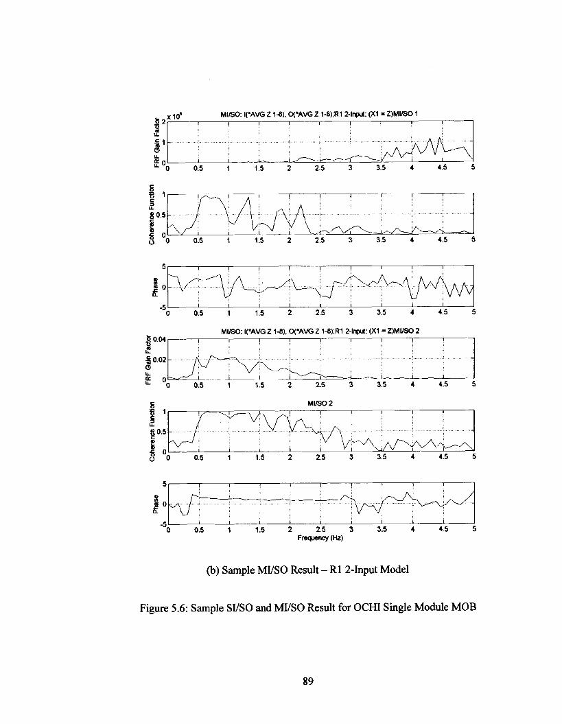
(b) Sample MVSO Result - R1 2-Input Model
b2'16 MIISO: I(*AVG Z l a ) , O(*AVG Z 1-8),R1 2-lnprrt: (Xi s Z ) M W I
Figure 5.6: Sample SVSO and MI/SO Result for OCHI Single Module MOB
2 u T- U.
I I I I I I I I
- - !E O 0 o . s I 1 5 - 2 2.5 3
-NqJ+ 3.5 4 4.5 5

The results in Table 5.5 can be seen to vary from the results obtained from the
MOB-Animate program. The discrepancy is due to the fact that values obtained using
the MOB-Animate program are visual and are based on dominant mode shapes at a
particular frequency. The SYSO and MYSO analyses are a relationship between the
input and output power. The roll response is below the 0.3 Hz range. Significant heave
and pitch responses are above the 0.6 Hz range. Comparing this with Table 5.4, the
heave and pitch have peak mode shapes at 0.64349 Hz and 0.70199 Hz respectively.
The linear SYSO results indicate that the heave is most influenced by the wave at
0.547 Hz, while the pitch is most influenced by the wave at 0.859 Hz. It is observed
that the pitch response frequency is in a highly elastic response range. This
undesirable response is created by the wave and is not a fundamental mode shape of
the single MOB module. The SYSO roll response is insignificant in the frequency
indicated in Table 5.5.
Improvement in the coherence function after applying a nonlinear model is the
indication of nonlinear behavior in the response. Studying the nonlinear characteristics
using the Direct MYSO results (see appendix D Figures D.8-D1.l l), the wave-heave
response does not show an improvement in the coherence when the difference in
velocities is used as a nonlinear input term (model Dl) in the MYSO analysis in the
region of 0.547 Hz. The same characteristic is also seen in the three-input model with
pitch as the third input. Since there is no significant improvement in the coherence, it
can be concluded that the wave-heave response does not have any significant
nonlinear characteristics. Similarly there is no significant improvement is observed in
the coherence for the wave-pitch response (model D2) in the region of 0.859 Hz.

The Reverse MYSO results (see appendix D Figures Dl. 12-Dl. 1 9 , there is
significant improvement in the coherence value in the range of 0.5 Hz to 2.5 Hz for
the reverse two models (models R1 and R2) suggesting a nonlinear damping force.
The three input models do not show any fiu-ther improvement to the two input models.
Hence the reverse nonlinear models applied should be considered when defining the
response of the MOB module in the range of 0.5 to 2.5 Hz range.
5.2.2 Results for Bretschneider BOW66 (b) Quartering Sea 2-58per 1125 RPM Data Set
The time history of the wave input and its frequency response is shown (Figure 5.7). It
can be seen that the input power is in the region of 0.23Hz to 1.9Hz with peak at
0.78 1 Hz. There is no significant input power below or beyond this range.
Time History
(a) Bretschneider Wave Time History
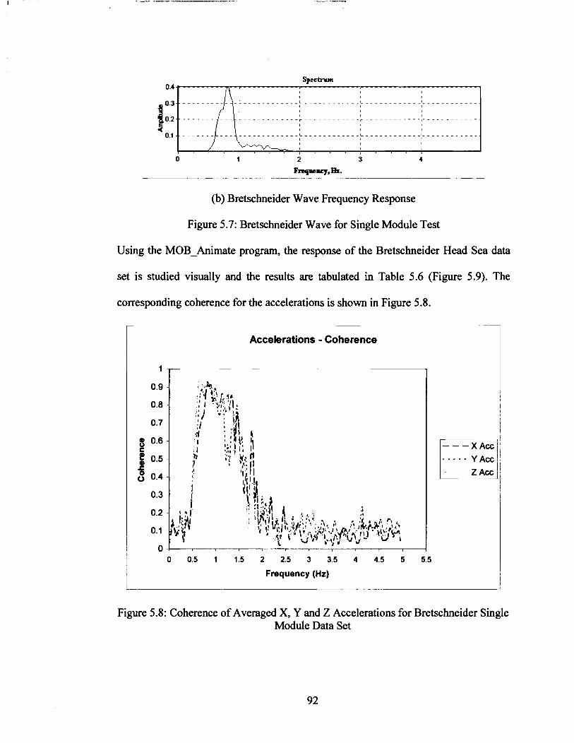
Spectrum
-- - - - - - - --
(b) Bretschneider Wave Frequency Response
Figure 5.7: Bretschneider Wave for Single Module Test
Using the MOB-Animate program, the response of the Bretschneider Head Sea data
set is studied visually and the results are tabulated in Table 5.6 (Figure 5.9). The
corresponding coherence for the accelerations is shown in Figure 5.8.
Accelerations - Coherence
- .- -
0 0.5 I 1.5 2 2.5 3 3.5 4 4.5 5 5.5
Frequency (Hz) - - -
Figure 5.8: Coherence of Averaged X, Y and Z Accelerations for Bretschneider Single Module Data Set

Table 5.6: Summary of Results for the Bretschneider Single Module
Frequency I Period 1 Response (Hz) / (seconds) I
0.09749 10.25 0.23399 Sway and
0.27299 Heave and
0.29 - 0.60
and Surge 0.66299
0.7 -1.28 1 1.38- I Mixed
3.45 - 1.67 Surge
Torsion,
1.51
Faint I Type I Coherence
Surge and ,Heave
Heave, Roll
1.28699
0-0.2 (poor) Response
* Surge
*
*
0.78125 0.78
I response I (moderate)
Non- elastic
response region (mild) Elastic
No response
I elastic 1 *
response region
(pronounc ed)
* I Highly 1 0.5-0.95
region Non- 0.95 (high)
I response I (moderate) *
It can be seen fiom Table 5.6 that surge, roll and heave are the significant
motions of the Bretschneider MOB single module model. As the orientation is
quartering seas, there is very good roll response of the structure, while the pitch and
yaw response are not significant. There is no response above 1.29 Hz. The structure
shows an elastic behavior in the 0.29-0.6 Hz and 0.8-1.28 Hz regions. This elastic
behavior, as in the OCHI single module case, cannot be concluded as being that of the
MOB model. Given the uniformity of the sensor motions it is highly probable that the
response is elastic in those ftequency ranges. Surge, roll and sway dominate the initial
non-elastic response region at 0.09749 Hz and 0.23399 Hz. There is a prominent
Elastic No
(high) 0.75

torsion observed in the region of 0.29 to 0.6 Hz along with heave and surge. Heave,
roll and surge have a pronounced mode shapes at 0.66299 Hz. Between 0.7 to 1.28 Hz
the response is mixed with no response beyond 1.29 Hz.
(a) Surge (0.09749 Hz) (b) Sway and Roll (0.23399 Hz)
(c) Heave and Surge (0.27299 Hz)

- - - - - - -- - - - - -- --
(d) Torsion (twist), Heave and Surge (0.29 - 0.60 Hz)
(e) Roll, Heave and Surge (0.66299 Hz)
Figure 5.9: Mode Shapes of the Single Module Bretschneider MOB
Using the DynanlicData program with a window length of 128 and an overlap
of 50, there were 13 records available for SVSO and MVSO analysis. The sampling
rate of the reduced data set is 10 Hz (period = 0.lsec). Sample SVSO and MIISO
results are shown (Figure 5.10). See appendix D2 for all figures related to SVSO and
MVSO analysis. The summary of results is presented in Table 5.7.

Table 5.7: SYSO and MYSO Results for the Bretschneider Single Module MOB
I
FWD WHT 1 0.469 - 1.953
SlSO W P 0.000 - 3.203
(Y = R). 2 0.000 - 2.422 D7 2-Input: (Y = P) 1 0.000 - 3.047 D7 2-Input: (Y = P) 2 0.000 - 2.266 R5 2-Input: (Xl = Z) 1 1.484 - 5.000
-
- - -
- - - - -
-
-
-
-
-
-
-
-
-
-
-
- * Maxfiequency represents the peaks corresponding to maximum coherence where
applicable; period is the inverse of the maximum_fi.equency value
Other significant Frequencies (Hz)

-5 I I I 1 I I I I I I 0 0.5 1 1.5 2 2.5 3 3.5 4 4.5 5
(a) SI/SO Input = FWD-WHT Output = Average Z
lX1O') SIISO I(FWD WHT). O(*AVG Z 1-8)
H L
P5 L
I I I I I I I I I
-J d"-\ d
Od 0:s I I I I 1 I
1 1 5 2 2.5 3 3.5 4 4.5 5

(b) Reverse Two-Input Model R5
Figure 5.10: Sample SYSO and MYSO Results for Bretschneider Single Module MOB
8 4 ~ 1 * MIISO: I(*AVG Z l a ) , WAVG Z 1-8);R5 2-Input: (Xi = Z)MVSO 1
ti G
j2 LL
I I I I I I I I
. . . . . . . . . . . . . . . . . . . . . . . . . . . . . . . . . . . . . . . . . . . . . . . . . . . . . . . . . . . . . . . . . . . . . . . . . . . . . . . . . . . . . . . . . . . . . . . . . . . . . . . . . . . . . . . . . . . . . . . . . . . . . . . !J\
-. ..; . , . . . .< . . . _
I I I --=L 2 - 7 I I ' Oo 015 1 1.5 2 2.5 3 3.5 4 4.5 5

As in the case of the OCHI MOB module, the results in Table 5.7 can be seen
to vary from the results obtained from the MOB-Animate program in Table 5.6. It can
be seen that the significant heave and pitch responses above the 0.6 Hz range while the
roll response is now both 0-0.3 Hz and in the 0.6-0.8 ranges. Both these ranges
correspond to the non-elastic response region shown in Table 5.6. Therefore it can be
concluded that the heave and roll have fimdarnental mode shapes at 0.66299 Hz. The
linear SVSO results indicate that the heave is most influenced by the wave at 0.781
Hz. The pitch is most influenced by the wave at 0.859 Hz as it is in the OCHI case,
which again is in an undesirable highly elastic response range. The SVSO roll
response is significant in the 0.781 Hz shown in Table 5.7.
Studying the nonlinear characteristics using the Direct MVSO results (see
appendix D Figures D.23-D.25), the wave-heave response does not show an
improvement in the coherence when the difference in velocities is used as a nonlinear
input term (model D5) in the MVSO analysis in the region of 0.781 Hz. Since there is
no significant improvement in the coherence, it can be concluded that the wave-heave
response does not have any significant nonlinear characteristics. Similarly, there is no
significant improvement observed in the coherence for the wave-roll response (model
D6) and wave-pitch response (model D7) in the region of 0.781 and 0.859 Hz
respectively.
The Reverse MIISO results (see appendix D Figures D.26-D.28) there is
significant improvement in the coherence value after 0.5 Hz for all the three models
(models R5, R6 and R7). As in the case of the OCHI, this suggests a nonlinear

damping force and the reverse nonlinear models have to be considered in analysis of
the Bretschneider data for frequencies greater than 0.5 Hz.
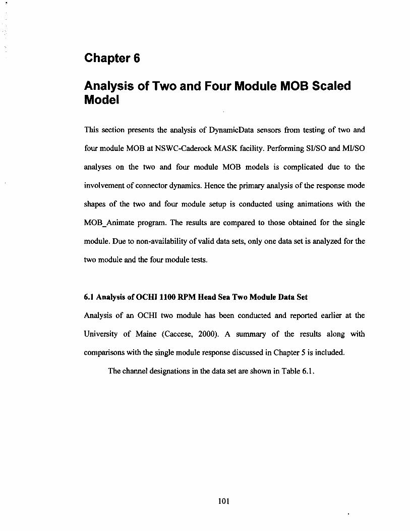
Chapter 6
Analysis of Two and Four Module MOB Scaled Model
This section presents the analysis of DynamicData sensors from testing of two and
four module MOB at NSWC-Caderock MASK facility. Performing SUSO and MUSO
analyses on the two and four module MOB models is complicated due to the
involvement of connector dynamics. Hence the primary analysis of the response mode
shapes of the two and four module setup is conducted using animations with the
MOB-Animate program. The results are compared to those obtained for the single
module. Due to non-availability of valid data sets, only one data set is analyzed for the
two module and the four module tests.
6.1 Analysis of OCHI 1100 RPM Head Sea Two Module Data Set
Analysis of an OCHI two module has been conducted and reported earlier at the
University of Maine (Caccese, 2000). A summary of the results along with
comparisons with the single module response discussed in Chapter 5 is included.
The channel designations in the data set are shown in Table 6.1.

Table 6.1 : Channel Designations in the OCHI Two Module Data Set
(a) Hydrodynamic Data Channel Designations
Response Designation FWRWVHT-2 ACCl X,Y,Z ACC2 X,Y,Z ACC3 X,Y,Z ACC4 X,Y,Z ACC5 X,Y,Z ACC6 X,Y,Z ACC7 X,Y,Z ACC8 X,Y,Z ACC9 X,Y,Z ACC 10 X,Y,Z ACC 1 1 X,Y,Z ACC12 X,Y,Z ACC 1 3 X,Y ,Z ACC 14 X,Y ,Z ACC 1 5 X,Y ,Z ACC16 X,Y,Z
Description Forward Wave Height - STBD
X,Y ,Z ~ccelerometer 1 X,Y,Z Accelerometer 2 X,Y,Z Accelerometer 3 X,Y,Z Accelerometer 4 X,Y,Z Accelerometer 5 X,Y,Z Accelerometer 6 X,Y,Z Accelerometer 7 X,Y,Z Accelerometer 8 X,Y,Z Accelerometer 9 X,Y,Z Accelerometer 10 X,Y,Z Accelerometer 1 1 X,Y,Z Accelerometer 12 X,Y ,Z Accelerometer 13 X,Y ,Z Accelerometer 14 X,Y ,Z Accelerometer 1 5 X,Y ,Z Accelerometer 16
(b) Connector Force Data Channel Designations
Connector Designation TLPinl PORT B L P ~ ~ ~ ~ P O R T TransPin4-PORT VERTPin3-PORT VertPin9-STBD TransPin 12-STBD BLPin2-STBD TLPinlO STBD
Ch. No. 5 3
137-39 140-42 143-45 146-48 149-5 1 152-54 155-57 1 5 8-60 26 1 -63 264-66 267-69 270-72 249-5 1 252-54 255-57 258-60
Description Top Longitudinal Pin, Port Side
Bottom Longitudinal Pin, Port Side Transverse Pin, Port Side
Vertical Pin, Port Side Top Longitudinal Pin, Starboard Side
Bottom Longitudinal Pin, Starboard Side Transverse Pin, Starboard Side
Vertical Pin, Starboard Side
Ch. No. 20 1
The original data set contains 272 channels sampled at 100 Hz. for a total of
72,000 data points with a sampling period of 720 seconds. The following reduction
scheme was applied:
Filter data - a 30 pole FIR filter is used with cutoff of 1/20 of the sampling
frequency. The average value is calculated and subtracted from the data set.

Decimate data by a factor of 20, resulting in an effective sampling rate of 5 Hz
and a Nyquist frequency of 2.5 Hz.
Compute the power spectral density (PSD) using a 256 point FFT, a Harming
window, and an overlap of 50% to get 27 records.
Compute FRF - the frequency response functions were computed. Reference
channel selected was the wave height sensor FWD-WHT-2 (channel 53), a
Hanning window, and an overlap of 50% resulting in 27 total records.
The reduced data is then exported to be W e r processed by EXCELTM and
MOB-Animate program. The input OCHI wave is shown (Figure 6.1). The input
power response is between 0.25 to 1.25Hz with a peak response at 0.43Hz. The
corresponding coherence for the output accelerations is shown in Figure 6.2. Using the
MOB-Animate program, the response of the OCHI Head Sea data set is studied
visually and the results are tabulated in Table 6.2 (Figure 6.3).
Tinle History
(a) OCHI Wave Time History

-- -- - -- -- --
(b) OCHI Wave Frequency Response
Figure 6.1 : OCHI Wave for Two Module Test
Accelerations - Coherence
- --
X Acc
Figure 6.2: Coherence of Averaged X, Y and Z Accelerations for OCHI Two Module Data Set

Table 6.2: Summary of Results for OCHI Two Module MOB
I)) 0.13649
Frequency (Hz)
Significant I Faint Res nse Response
+sway
Period (seconds)
Pitch, Heave Pitch and
Response
Sway Connector Heave
angle and out- of-phase
Sway Pitch and Heave
Connector * angle and in-
hase Swa
response
Type
Irregular rigid
response region (mild)
Rigid response
Elastic response
No significant response
Coherence
0.1-0.6 (moderate)
0.15 (Poor)
It can be seen from Table 6.2 that sway is the significant motion of the OCHI
MOB two module model. As the orientation is head seas, there is poor roll response of
the structure and absent yaw response. There is no significant response above 1.29 Hz.
The structure shows elasticity in the 0.99- 1.13 Hz region. Comparing this to the single
module, it is observed that the two module configuration shows less elasticity than the
single module. This could be due to the flexibility offered by the connectors. The
primary mode shape of surge is between 0.13-0.17 Hz with faint swaying or rolling.
There is a combined pitch and heave response at 0.22 Hz. There is a sway response

(in-phase and out-of-phase) over a wide range from 0.23 to 0.75Hz. At 0.23Hz it is
combined with pitch. Between 0.25 and 0.6Hz the surge is out-of-phase and is
combined with the connector angle mode shape. At 0.66Hz the response is dominated
by the sway with faint pitch and heave response. At 0.74 Hz there is a in-phase sway
response with connector angle. Between 0.99 Hz and 1.13 Hz, the model shows a high
elastic response with out-of-phase torsion (twisting) of the two modules constrained
by the connectors.

(a) In Phase Pitch and Sway (0.23399 Hz)
(b) Connector Angle and Out-of-Phase Sway (0.42899 Hz)

(c) Pitch and Heave Response Combined (0.50699 Hz)

-- --
(e) Out of Phase Torsion Con&ained by the ~ ~ ~ & t o r s (0.99 Hz)
Figure 6.3: Mode Shapes of OCHI Two Module Test
Figure 6.4 show the connector response on the port side and starboard side. It
can be seen that connector response range is dominant between 0.1 to 0.7 Hz with
maximum force between 0.23Hz to 0.5Hz and a peak at 0.43Hz. This corresponds to
the peak of the wave height frequency response (Figure 6.1) and the in-phase and out-
of-phase sway and connector angle response (Table 6.2).

Port Side Connector Response
(a) Port Side Connector Response
StarBoard Connector Response
0 0.25 0.5 0.75 1 1.25 1.5 1.75 2
Frequency (W
(b) Star Board Side Connector Response
Figure 6.4: Connector Response of the OCHI Two Module Test

6.2 Analysis of Bretschneider 1125 RPM 85DEG Quartering Sea Four Module Data Set
The channel setup for the Bretschneider quartering sea data is shown in Table 6.3.
Table 6.3: Channel Designations in the Bretschneider Quartering Sea Data
(a) Hydrodynamic Data Channel Designations
Response Designation F WD-WVHT-2 ACCl X,Y,Z ACC2 X,Y,Z ACC3 X,Y,Z ACC4 X,Y,Z ACC5 X,Y,Z ACC6 X,Y,Z ACC7 X,Y,Z ACC8 X,Y,Z ACC9 X,Y,Z ACC 10 X,Y,Z ACC 1 1 X,Y,Z ACC 12 X,Y,Z ACC13 X,Y,Z ACC14 X,Y,Z ACCl5 X,Y,Z ACC 16 X,Y,Z ACC 17 X,Y,Z ACC 18 X,Y,Z ACC 19 X,Y,Z ACC2O X,Y,Z ACC21 X,Y,Z ACC22 X,Y,Z ACC23 X,Y,Z ACC24 X,Y,Z ACC25 X,Y,Z ACC26 X,Y,Z ACC27 X,Y,Z ACC28 X,Y,Z ACC29 X,Y,Z ACC30 X,Y,Z ACC3 1 X,Y,Z ACC32 X.Y.Z
Description Forward Wave Height - STBD
X,Y,Z Accelerometer 1 X,Y,Z Accelerometer 2 X,Y,Z Accelerometer 3 X,Y,Z Accelerometer 4 X,Y,Z Accelerometer 5 X,Y,Z Accelerometer 6 X,Y,Z Accelerometer 7 X,Y,Z Accelerometer 8 X,Y,Z Accelerometer 9
X,Y,Z Accelerometer 10 X,Y,Z Accelerometer 1 1 X,Y,Z Accelerometer 12 X,Y,Z Accelerometer 13 X,Y ,Z Accelerometer 14 X,Y,Z Accelerometer 15 X,Y ,Z Accelerometer 16 X,Y,Z Accelerometer 17 X,Y ,Z Accelerometer 1 8 X,Y,Z Accelerometer 19 X,Y,Z Accelerometer 20 X,Y,Z Accelerometer 2 1 X,Y,Z Accelerometer 22 X,Y,Z Accelerometer 23 X,Y,Z Accelerometer 24 X,Y,Z Accelerometer 25 X,Y,Z Accelerometer 26 X,Y,Z Accelerometer 27 X,Y,Z Accelerometer 28 X,Y,Z Accelerometer 29 X,Y,Z Accelerometer 30 X,Y,Z Accelerometer 3 1 X,Y,Z Accelerometer 32
Ch. No. 5 3
137-39 140-42 143-45 146-48 149-5 1 152-54 155-57 1 58-60 26 1-63 264-66 267-69 270-72 249-5 1 252-54 255-57 258-60 4 1-43 44-46 47-49 50-52 53-55 56-57 59-6 1 62-64 9-1 1 15-17 12-14 18-20 2 1-23 24-26 27-29 30-32

(b) Connector Force Data Channel Designations
Connector Designation TLPinl PORT B L P ~ ~ ~ ~ P O R T TransPin4-PORT VERTPin3-PORT VertPin9-STBD Transpin 12-STBD BLPin2-STBD TLPinlO STBD
Description Top Longitudinal Pin, Port Side
~ o t & m Longitudinal Pin, Port Side Transverse Pin, Port Side
Vertical Pin, Port Side Top Longitudinal Pin, Starboard Side
Bottom Longitudinal Pin, Starboard Side Transverse Pin, Starboard Side
Vertical Pin, Starboard Side
Ch. No.
206 207 208
The original data contains two files. One set containing 272 channels sampled
at 100 Hz. for a total of 46,080 data points with a sampling period of 460 seconds. The
other data set contains 64 channels sampled at 100 Hz with the same number of data
points and sampling period. The following reduction scheme was applied:
Filter data - a 30 pole FIR filter is used with cutoff of 1/20 of the sampling
frequency. The average value is calculated and subtracted from the data set.
Decimate data by a factor of 20, resulting in an effective sampling rate of 5 Hz
and a Nyquist frequency of 2.5 Hz.
Compute the power spectral density (PSD) using a 256 point FFT, a Hanning
window, and an overlap of 50% to get 9 records.
Compute FRF - the frequency response functions were computed. Reference
channel selected was the wave height sensor FWD-WHT-2 (channel 53), a
Hanning window, and an overlap of 50% resulting in 9 total records.
The reduced data is then exported to be further processed by EXCELTM and
MOB-Animate program. The input Bretschneider wave is shown (Figure 6.5). The
input power response is between 0.25 to 0.9Hz with a peak response at 0.43Hz. The

acceleration data across the different data sets had different scaling factors. A scaling
scheme was used to normalize the data (see appendix E for scaling technique
adopted). The corresponding coherence for the accelerations is shown in Figure 6.6.
Using the MOB-Animate program, the response of the Bretschneider quartering sea
data set is studied visually and the results are tabulated in Table 6.4 (Figure 6.7).
Time History
(a) Bretschneider Wave Time History
(b) Bretschneider Wave Frequency Response
Figure 6.5: Bretschneider Wave for Four Module Test

Accelerations - Coherence
Figure 6.6: Coherence of Averaged X, Y and Z Accelerations for Bretschneider Four Module Data Set

Table 6.4: Summary of Results for Bretschneider Four Module MOB Data Set
Frequency I Period Response (HZ) I (seconds) I
Roll 0.23399 4.28
0.272999 0.3 1 - 0.60
without Roll) 1 .56 and 0.64 No significant
Surge Sway, Heave,
0.72 149
above response
3.66 3.23 - 1.67
Faint I Type I Coherence
Heave, Roll Surge, Heave,
1.39 Roll, Torsion In-phase Roll
Surge I region I
Response Roll
~ -
Irregular
Sway *
I I * No 1 0.2 (poor)
0.1 - 0.4
Heave and Surge
I significant I
Elastic
I response I
0.3-0.85 response
Rigid response
It can be seen from Table 6.4 that surge is the significant motion of the
Bretschneider MOB four module model. As the orientation is quartering seas, there is
good roll and torsion response of the structure. There is no significant response above
1.56 Hz, which is higher than the response range seen in the one and two module
cases. The structure shows elasticity in the 0.3-0.6 Hz and 0.7-1.56 Hz regions. The
primary mode shape in the initial frequency range is the in-phase surge at 0.0975Hz. A
(hlgh) 0.75
(hight) * Elastic
response
combined sway, heave and roll response is observed at 0.234Hz. A heave and roll
combination is observed at 0.273I-I~. The frequency range between 0.3 to 0.6 Hz is
dominated by a combination of surge, heave, roll and torsion, which is in the primary
frequency response region of the wave. There is significant roll response with in-phase
0.2-0.65 (moderate)

roll at 0.72Hz and out-of-phase roll at 0.799Hz. There is a significant surge response
between 0.76-1 S6Hz frequency range. There is no significant response above 1.56Hz.
(a) In-phase Surge (0.09749 Hz)
(b) Roll, Sway and Heave (0.23399 Hz)

(c) Surge, Roll, and Heave (0.42899 Hz)
---%4-
(d) Out-of-Phase Roll (0.79949 Hz)
117

(e) Out-of-phase Surge (0.87749 Hz)
Figure 6.7: Mode Shapes of the Bretschneider Four Module MOB
There is only one set of connector force sensors available in the data set.
Figure 6.8 shows the connector response on the port and starboard side. It can be seen
that connector response range is dominant between 0.1 to 1 Hz with maximum force
around 0.43Hz. This corresponds to the peak wave frequency (Figure 6.5) and elastic
response region dominated by surge, roll and heave in a torsion motion (Table 6.4).

Port Side Connector Response
(a) Port Side Connector Response
StarBoard Connector Response
- - - - -- . .-
- TLPinl PORT - BLPinS PORT
T ranstin4 PORT --VERTPin3 PORT
(b) Star Board Connector Response
Figure 6.8: Connector Response of a Bretschneider Four Module Test

Chapter 7
Summary, Conclusions, and Future Work
This chapter summarizes the thesis work and presents conclusions. The future directions
for research based on this work are highlighted with recommendations.
7.1 Summary
The overall goal of this thesis was to provide necessary validation data to develop
hydrodynamic and hydroelastic computer models for the analysis of critical MOB
aspects. The response frequency mode shapes are analyzed and provided for the single,
two and four module hydrodynamic scale model tests for available data sets. Results
indicate the response of the MOB scale module to be elastic in nature. The nonlinear
characteristics of the single module are also investigated. MLISO results indicate the
development of a nonlinear damping force in the MOB module.
7.2 Conclusions
The following conclusions are outcome of this thesis work:
At any given frequency, the response of a module is generally described by a
combination of mode shapes. The motion is rarely described using one particular
mode shape alone.
The response of the module is elastic. Significant torsion is observed in the
Bretschneider single module, OCHI two module and Bretschneider four module
configurations that depict the elastic motion response.

The response of the modules is highly dependent on the kind on input wave. Poor
roll response is observed in OCHI head seas, while the Bretschneider quartering
seas show significant roll response at specific frequencies.
High roll response is observed in quartering seas in the region of 0.6 to 0.8 Hz for
single module Bretschneider case and 0.6 to 1.2 Hz region for the multi module
case. This can be combined with a torsion response.
In-phase and out-of-phase torsion is observed to be significant in both the two and
four module case.
Sway is observed to be the significant response type of a two module OCHI
configuration.
Surge is observed to be the significant response type of a four module
Bretschneider configuration.
A higher response range is observed in the four module case compared to the
single and two module configurations.
While no nonlinearity is observed in Direct MUSO models (wave influence on the
module), good nonlinearity is present in Reverse MUSO models that suggest the
presence of a nonlinear damping force.
7 3 Future Work
This section reviews the future work that the efforts of this thesis can lead:
Development of hydrodynamic and hydroelastic models
In keeping with the objectives of this thesis, the frequency mode shape values can
be used to develop hydrodynamic and hydroelastic computational models. Several

commercial finite element analysis programs, namely ABAQUSa and Algofi,
have built in hydroelastic elements that can be used in creating the models. The
input wave can be specified and the output response for a particular finite element
model can be made to match the values provided by this research work.
Conducting further scale model testing
One of the primary constraints in the analysis of a MOB scale model response
was the lack of sufficient data sets. Further testing can be carried out for different
wave models for the single, two and four model configurations. In designing
future tests, the following aspects need special attention:
o Run lengths should be sflcient so that the initial transient effects can be
removed from the time history, while having enough records for better
averaging of results. At the same time, care should be taken to prevent
lengthy data collection that might be affected by wave reflections.
o Proper calibration data for all the sensors should be available. This study
did not concern itself with the amplitudes of the responses. In order to
facilitate the study of the amplitudes of the response, properly scaled and
referenced acceleration data need to be made available.
o Sufficient runs must be made for head, beam and quartering seas.
o Wider random spectra should be utilized for three sets of seas - head,
beam and quartering at different amplitudes.

BIBLIOGRAPHY
Taylor, R.L. and Zueck, R.F., "Mobile Offshore Base - A Self Propelled Logistics Platform", Logistics Spectrum, SOLE, Vol. 35, Issue 1, January - March 200 1.
Weybrant, E., 1999, "A computational study of connector force dynamics in a mobile offshore base (MOB)", dissertation at the University of Maine, Orono.
Remrners, G., Zueck, R., Palo, P., and Taylor, R., "Mobile Offshore Base", presented at ISOPE, Montreal, May 1997.
Sikora, J., and Smith, T., 1998, "Test plan for MOB Model Tests", NSWCCCD, Third Draft.
Zueck, R., Taylor, R. and Palo, P. "Development Options for Mobile Offshore Base Technology", The 1 lh International Offshore and Polar Engineering Conference, Stavanger, Norway, June 200 1.
,
Smith, T.C., O'Dea, J., and Lewis, R., January, 1998, "Mobile Offshore Base Motions and Connector Loads Data Reduction", Naval Surface Warfare Center Report CRDKNSWCIHD-0279- 10.
Blevins, R.D., 1977, "Flow-induced vibration", Van Nostrand Reinhold Company.
Blevins, R.D., 1979, "Structural Vibrations in a Fluid", Chapter 14 fiom "Formulas for Natural Frequency and Mode Shapes", Van Nostrand Reinhold Company.
Ban, R.A., November 10,1999, "Review of NSWCCD Mask Wave Test Data for use in MOB Tests", Technical Note 9920-1, Hydronautics Research, Inc.
McCormick, M.E., 1973, "Ocean Engineering Wave Mechanics", Wiley- Interscience Publication.
Wilson, J.F., 1984, "Dynamics of Offshore Structures", Wiley-Interscience Publication.
Ochi, M.K., 1998, "Ocean Waves: The Stochastic Approach", Cambridge University Press.

Zhang, J., 1998, "Ocean Wave Kinematics, Dynamics and Loads on Structures", Proc. of the 1998 International OTRC Symposium, ASCE.
Berteaux, H., "Buoy Engineering", UMI Books on Demand, 1994, originally published by John Wiley & Sons, 1976. Caccese, V., February 2000, "Dynamic Response of the Mobile Offshore Base Hydroelastic Test Model", Technical Progress Report, Department of Mechanical Engineering, University of Maine, Orono, USA.
Riggs, H. R., "Current Efforts in Technology Development for Very Large Floating Structures", First International Workshop on Very Large Floating Structures, Honolulu, April 199 1.
Sarpkaya, T., and Isaacson, M., 1981 "Mechanics of Wave Forces on Offshore Structures", Van Nostrand Reinhold Company.
Ochi, M. K., and Hubble, E. N., 1976, On six-parameter wave spectra. Proc. 15th Coastal Engineering Conf , A.S. C. E., 32 1 -328.
Allemang, R. J., 1995, Vibrations: Experimental Modal Analysis; Structural Dynamics Research Laboratory; University of Cincinnati; UC-SDRL-CN-20- 263-6631664; Cincinnati, Ohio.
National Instruments, "Phase" and "Phase Measurements", Measurement Glossary.
Bendat, J.S., 1998, "Nonlinear systems techniques and applications", John Wiley and Sons, Inc.
Marven, C. and Ewers, G., 1996, "A Simple Approach to Digital Signal Processing", John Wiley and Sons.
Morgan, D., 1994, "Practical DSP - Modeling, Techniques, and Programming in C", John Wiley and Sons.
Bendat, J.S., and Piersol, A.G., 1986, "Random Data: Analysis and Measurement Procedures", John Wiley and Sons.
Wiener, N., 1949, "Extrapolation, Interpolation, and Smoothing of Stationary Time Series", published jointly by MIT Press and John Wiley and Sons.
Bendat, J.S., and Piersol, A.G., 1980, "Engineering Applications of Correlation and Spectral Analysis", John Wiley and Sons.
Bendat, J.S., 1990, "Nonlinear system analysis and identification from Random Data", John Wiley and Sons.

[28] Mathworks, 1999, "MATLAB Signal Processing Toolbox", Ver. 4, User's Guide.
[29] M.A. Corp, 2000, "Integrated Test Analysis Processor Toolbox User's Guide".

Appendix A
Non-Dimensional Parameters of a Two- Dimensional, Spring-Supported, Damped Structural Model Exposed to a Steady Flow (Blevins, 1977)
A.l Fineness ratio (non-dimensional geometry parameter)
Fineness ratio = L= Length Eq(A. 1)
D width
Width (D) - side normal to the free stream surface.
Length (L) - characteristic length along the free stream surface
A.2 Reduced Velocity (non-dimensional velocity parameter)
Reduced Velocity = U = path length -per cycle
fD Model width
U - free stream velocity
f - frequency of vibration (of structure in fluid)
The non-dimensional frequency is the inverse of reduced velocity.
A.3 Dimensionless Amplitude
Dimensionless Amplitude = A, = vibration amplitude h(A.3)
D model width
A.4. Mass Ratio
Mass ratio = = mass per unit length of model Eq(A.4)
p ~ 2 fluid density x model dimension
'm' includes structural and "added" mass

The mass ratio term is commonly used to measure the susceptibility of lightweight
structures to flow-induced vibration.
A S Reynold's Number (Re)
Re =UJ= inertial force Eq(A-5)
v viscous force (kinematic viscosity)
This ratio is used to determine the transition from laminar to turbulent fluid flow and
the boundary layer thickness.
A.6 Mach Number
Mach Number = U = fluid velocity . c velocity of sound
A.7 Damping FactorIRatio ( )
< = enervy dissipated -per cycle . 4n * total energy of the structure
A.8 Reduced Damping ( 6, )

A.9 Application of the non-dimensional parameters
The dimensionless amplitude is a hnction of fineness ratio, reduced velocity,
Reynolds's number, damping ratio, mass ratio.
A.10 Strouhal Number (S)
The Strouhal number is the non-dimensional frequency parameter. At low Mach
number flows it is a fimction of geometry and Reynold's number. Expression for
Strouhal's number is:
fs - frequency of vortex shedding (dominant)
U - free stream velocity
D - width (normal to free stream surface)
S - Strouhal number
Strouhal numbers for specific geometries are available. "Bluff sections" have lower
Strouhal numbers.
A.ll Froude Number (Fr)
Froude number is proportional to the inertial force over the gravitational force and is
used in momentum transfer in general and open channel flow and wave and surface
behavior calculations in particular. It is normally defined in one of the following forms
Fr = 2 (or) 2 Eq(A.11)

where a - Acceleration g - Gravitational acceleration L - Characteristic Length V - Fluid Velocity

Appendix B
Wave Spectrums
B.l Bretschnieder Wave Spectrum Example
H, := 12 Significant wave height (ft)
Ts := 6.9 Significant wave period (sec.)
1050 4
4200y2 S~H(T) := -e Bretschnieder Formula ftA2-sec
5
Bretschneider Double Height Spectra 300
200 - -
T

B.2 OCHI Wave Spectrum Example
OCHI Six-Parameter Soectrum

Appendix C
Integration and Differentiation Functions - MATLAB@ Code Listing
'$ DSI' - DIFF [ ) - F u n c t i o n 1-0 P e r f o r i r ~ D i f f e r e n t i a l i o n t,
f u n c t i o n [yf, vf, af] = dsp-diff(y, sfreq, FMax, Wn)
dt = l/sfreq; [m,n] = size(y); Time = [O:dt:m*dt-dt]';
i G e t v e l o c i t y v = diff(y)/dt; [P, ql = size (v) ;
; FFT f i l t e r the v e l o c i t y [vnew] = fftfil(v,FMax,Wn); [r,s] = size(vnew) ;
'+ G e t a c c e l e r a t i o n a = diff (vnew) /dt; [t, u] = size (a) ;
- Normalize t h e a c c e ! e r a t i o n [anew] = fftfil (a, FMax,Wn) ; [e,f] = size
Y F i n a l r e s a yf = Y vf = vnew af = anew
anew) ;
t s 1:e) ; 1:e); 1:e);

2 Dsp - i r ~ t ( ) - F u n c t i o n t o p e r f o r i c i n t e g r a t i n n o f dcl ta 3 I n t e g r a t i o n t - e c h n i q d e - c o n s t a n t a z z e l e r a t i o n metihod f
f u n c t i o n [yf, vf, af] = dsp-int(a, sfreq, FMax, Wn)
dt = l/sfreq; [m,n] = size(a); Time = [O:dt:m*dt-dt]';
% O b t a i n t h e v e l o c i t y v = zeros (m, 1) ; f o r i=l: (m-1)
dt = Time (i+l, 1) -Time (i, 1) ; da = a(i+l,l) - a(i,l); dv = a(i,l)*dt + 0.5*da*dt; v(i+l, 1) = v(i, 1) + dv;
e n d
h FFT f i l t e r the v e l o c i t y [vnew] = fftfil (v, E'Max,Wn) ; [p, ql = size (vnew) ;
8 O b t a i n t h e d j sp l a c e m e n t f r o m t h e f i l t e r e d v e l . o c i t y y = zeros (p, 1) ; f o r i=l: (p-1)
dt = Time (itl, 1) -Time (i, 1) ; dvnew = vnew(it1,l) - vnew(i,l); dy = vnew(i,l)*dt + 0.5*dvnew*dt; y(it1,l) = y(i,l) + dy;
e n d
r FFT f i j t e r t h e d i s p l a c e r n e x L [ynew] = fftfil(y,EMax,Wn); [r, S] = size (ynew) ;
% Return r e s ~ l t af = a(1:r); vf = vnew(1:r); yf = ynew(1:r);

i fit - fll() - Function to F e r F o r m FFT f i L L e r l n g
functlon [v - new] = fftfil (v, maxfreq, remfreq)
m = length (v) ; fdt = maxfreq/m; freq = [fdt:fdt:m*fdt]; v fft = fft(v); v-f - ft - new = zeros (m, 1) ; rmlen = (maxfreq/remfreq)/Z; v - fit - new(rmlen+l:(m-rmlen)) = v - fft(rmlen+l:(m-rmlen)); v - new = real(ifft (v-fit-new));

Appendix D
Time History, SllSO and MllSO Results for Single Module MOB Scale Model Tests
D.l Bretschneider BOW66 (b) Quartering Sea 2-58per 1125 RPM Data Set
File: Ochi,d Chen:FWD WHT [dt=O.l. Nw=128, df=0.078. N,=Q. Mean=O.0015, Std=1.4] 02-.Id2001 11:53 PM
0 20 40 60 80 100 Time Standardized Variable
Figure D. 1 : FWD-WHT Time History (Input Power)

I I I 0 20 40 60 80 100
Time
Figure D.2: Heave (Average Z) Time History (Output Power)
1 ~ 1 $ S I M : I(WD WHT), O(*AVG Z 1-8)
V I I I I I I I I I
LL
5 OS .; . . . . ..... . ...... : ..... . . . . . . ... '... .. .... .. . . . .. .. ..".. ' "...: ' . ' . .-
LL
L 0 i 1- I I I I I
0 0.5 1 1.5 2 2.5 3 3.5 4 4.5 5
Figure D.3: SVSO Input = FWD-WHT Output = Average Z
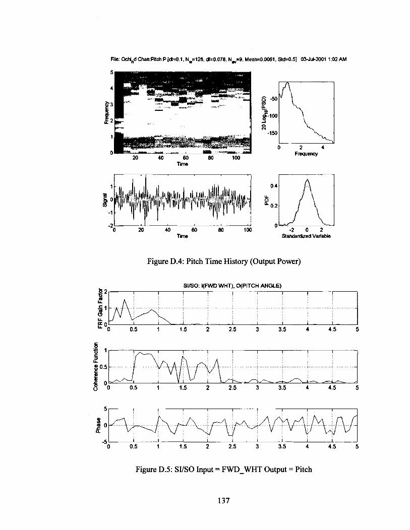
20 40 60 80 100 Time
-a
0 20 40 60 80 100 Time
0.2 0'4K 0
-2 0 2 Standardized Variable
Figure D.4: Pitch Time History (Output Power)
SIISO: I(FWD WHT). OlPlTCH ANGLE)
Figure D.5: SYSO Input = FWD-WHT Output = Pitch

File: M , d Chen:Rd R Id=O.l. N-428, m.078. N,4. Mean4.03. Std=0.38) 03-Jd2001 1:02 AM
Time
0 20 40 60 80 100 Time Standardized Variak
Figure D.6: Roll Time History (Output Power)
SlISO: I(FWD WHT), O(R0LL ANGLE) 10
2 I I I I I I I I I
u ............. . . . . . . . . . . . . . . . . . . . . . . . . . . . . . . . . . . . . . .; ...; ; ............ ...+ ...... . . . . . ' . . . . . ...: . . . . ' . . . . '.. '. .-
I 1 I I I I I I I
0.5 1 1.5 2 2.5 3 3.5 4 4.5 5
Figure D.7: SVSO Input = FWD-WHT Output = Roll

Phase Phase FRF G 1 Fada
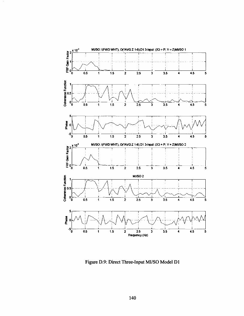
Figure D.9: Direct Three-Input MUSO Model Dl

MUSO' I(FWD WHT). O(PITCH ANGLE);D2 2-Input: (Y = P ) M W 2 b 0.04 V I I I I I I I I I
LL
LL 1 I
MVSO: I(FWD WHT), O(PITCH ANGLE);D2 2-Input: (Y = P)MI/SO 1 b 2
Figure D. 10: Direct Two-Input MIIS0 Model D2
V LL
z 1 LL
I I I I I I I 1 I
~ r u h - I LA--
"0 0015 1 1.5 2 2.5 3 3.5 4 4.5 5

MVSO: I(FWD WHT), O(PITCH ANGLE);D2 f lnplt. (X3 = P. Y = P)MIISO 1 2 -
% I I I I I 1 I I I
L -
--I I I I I I - 1 1.5 2 2.5 3 3.5 4 4.5 5
Figure D. 1 1 : Direct Three-Input MIISO Model D2

x 106 MIISO: I(*AVG Z l a ) , WAVG Z 1-8);Rl 2 - l w : (Xi = Z)MVSO 1 b 2
Figure D. 12: Reverse Two-Input MYSO Model R1
3 LL
C l - (3 LL
MIISO: I(*AVG Z l a ) , WAVG Z 14),Rl 2 - l w . (Xi = Z)MVSO 2 b 0.04
I I 1 I I I I I I
- -I-'-~Y--4-----l,
2 LL
LL
OO- 1 1 5 2 2.5 3 3.5 4 4.5 5
PA+"&<
I I I I I I 1 I I
- I 1 E oo 0.5 1 1.5 2 2.5 3 3.5 4 4.5 5
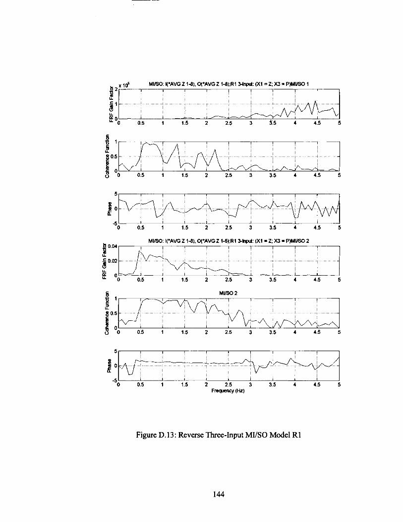
Figure D. 13 : Reverse Three-Input MIISO Model R1
MIISO: I('AVG Z 1-a), WAVGZ 1-8);Rl 3- I@: (Xl = Z; X3 = P)MVSO 2 b 0.04 3 LL 5 O m LL
I I I I I I I I I
- I ' J -7 I \"----
t Ood 0.5 I 1 I 1.5 I 2 I 2.5 I 3 3.5 4 4.5 1 ---LA-
S MISO 2

MVSO: I(PITCH ANGLE), O('AVG Z 1-8);R2 2-ltW: (XI = P)MVSO 1 b 100 P I I I I I I I I I I
MVSO: I(PITCH ANGLE), O('AVG Z 1-8);R2 2-1W-t: (XI = P)MVSO 2 g0.04, I ! ! I I I I I I 1
Figure D. 14: Reverse Two-Input MLISO Model R2
5
0
- I I I I I I I I I
T"J------ - - ~ , ~ v ~ ~ - ~ ~ - - 5 ~
I I I I I I I 1 I
0.5 1 1.5 2 2.5 3 3.5 4 4.5 5 Frequency (Hz)

MVSO: I(PITCH ANGLE), O(*AVG Z 1-8);R2 %I@: (Xi = P; X3 = P ) M W 2 I I I I
u C
u c oo 1 I d , I-- 1 I
0.5 1 1 .5 2 2.5 3 3.5 4 4.5 5
MIISO: UPITCH ANGLE), O(*AVG Z 1-8);RZ 3- I@: (XI = P; X3 = P ) M W 1
Figure D. 15: Reverse Three-Input MIIS0 Model R2
u
i so- u
I I I I I I I I I
- A ,'-' c 0, ---- ' J ' c q 0 5 1 1 .5 2 2.5 *yl%>~& 3 3.5 4 4.5 5

D.2 Bretschneider BOW66 (b) Quartering Sea 2-58per 1125RPM Data Set
File: FWD#T C h e n : w H T [dt=O.l . N,=l28, dl=0.078, N,=13, Mean=-0.0044, Std=3] 1 1-JIJI-2001 l2:XJPM
20 40 60 80 100 120 140 160 Time
-101 I 0 50 100 150
Time Standardized Variable
Figure D. 16: FWD-WHT Time History (Input Power)

Fib: Z Chan:Z [dt=O.l. N,,,=128, df--0.078, Nw=13, Mean=-le-006. Std=0.00093] 11-Jd2001 12:30PM
- --- .-A -. - - oEX-.-- c ._I -- 20 40 60 80 loo 120 140 160
Time x 10"
I I I 0 50 100 150
Time
0 2 4 Frequency
Standardized Variable
Figure D. 17: Heave (Average Z) Time History (Output Power)
SIISO: I(M WHT). WAVG Z 1-8) I I I I I I I I
-
I I I I I I
2 2.5 3 3.5 4 4.5 5
Figure D. 18: SVSO Input = FWD-WHT Output = Average Z

20 40 60 80 100 120 140 160 Time
50 100 150 Time
Frequency
-2 0 2 Standardized Variabk
Figure D. 19: Pitch Time History (Output Power)
SllSO: I(FWD WHTl OtPITCH ANGLE)
Figure D.20: SVSO Input = FWXWHT Output = Pitch
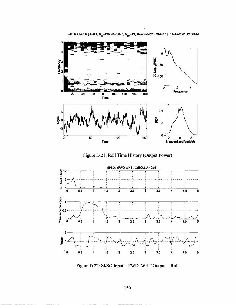
File: R Chan:R [dt=O.l. Nw=128, dkO.078. N,=13. MeensO.023. Stck3.11 11-JuC2001 1230PM
Time
Time Standardized Varlabk
Figure D.21: Roll Time History (Output Power)
SIJSO: I(FWD WHT), O(R0LL ANGLE) 10
ti I I I I I I I I I
-
u 1 - 1 I I I I I I
1 1.5 2 2.5 3 3.5 4 4 5 5
Figure D.22: SIISO Input = FWD-WHT Output = Roll

.x1o4 MVSO: I (WD WHT), O(*AVG Z 1-8);DS 2-Input: (Y = Z)MVSO 1
Figure D.23: Direct Two-Input Model D5
4~ lo4 MVSO: I ( W D WHT). O(*AVG Z 1-8);DS 2-Input: (Y = Z)MVSO 2
3 LL
(3 LL
I I I I I I I I I
-
"r/bLLL I I I
"0 0.5 1 1.5 2 2.5 3 3.5 4 4.5 5
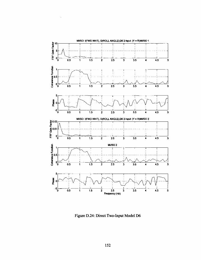
MIISO: I(FWD WHT). O(R0LL ANGLE);DG 2-Input: (Y = R)MVSO 1
(3 LL
'0 0.5 1 1.5 2 2.5 3 3.5 4 4.5 5
Figure D.24: Direct Two-Input Model D6

MVSO: I(FWD WHT), QPITCH ANGLE);D7 2 - lW: (Y = P)MIISO 1 8 2 V I I I I I I I I I
LL -
' I I I I
1 1 5 2 2.5 3 3.5 4 4.5 5
MVSO: I(FWD WHT), QPITCH ANGLE);D7 2 - l W : (Y = P)MVSO 2 I I I I I I I
1 I I I I
0.5 1 1.5 2 2.5 3 3.5 4 4.5
Figure D.25: Direct Two-Input Model D7

Figure D.26: Reverse Two-Input Model R5
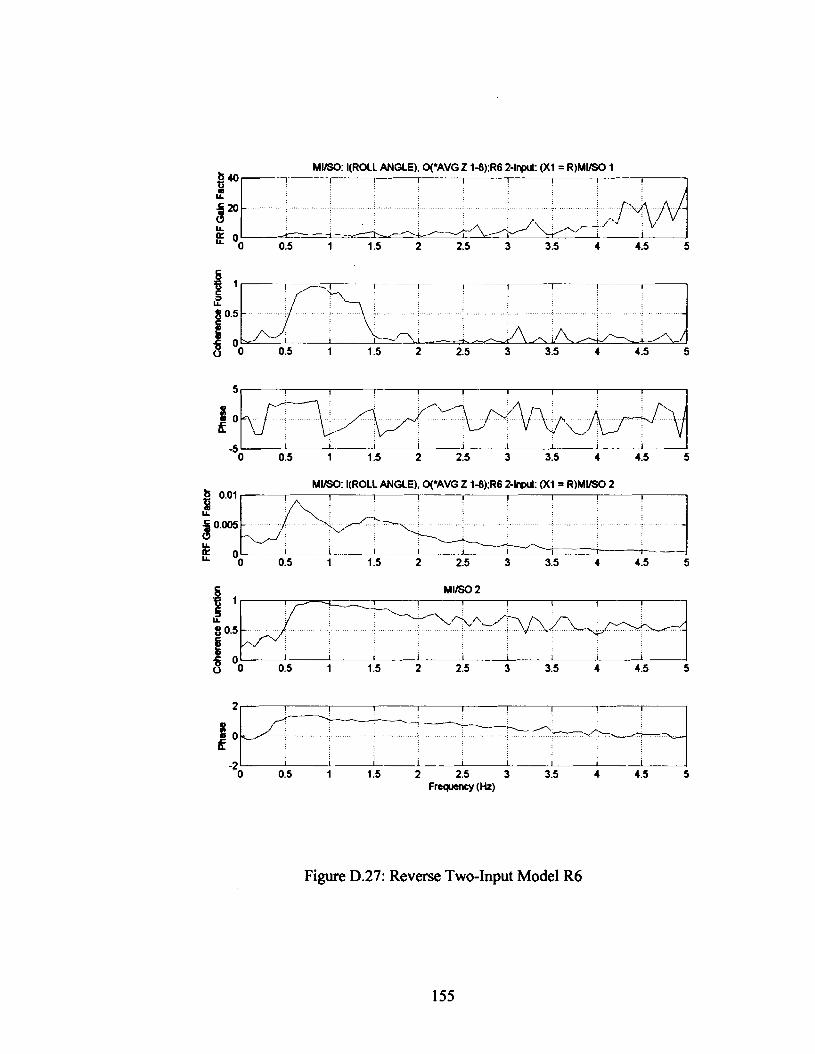
MVSO: I(R0LL ANGLE). WAVG Z 1-8);R6 2-lnpllt: (Xi = R)MVSO I ba V I I 1 I I I I I I
LL . .................................................. . . . . . . . . . . . . . . . . . . . . . . . . . . . . . . . . . . . . . . . . . . . g - . j . . . . . . ', "\,v:
9 . . LL
1
0.5 I 1.5 2 2.5 3 3.5 4 4.5 5
MVSO: I(R0LL ANGLE), WAVG Z 1-8);R6 2-lrpllt: (Xi = R)MVSO 2
........... . . . . . . . . . . . . . . . . . . . . . ......... ' . . . . . . . . . . . . ..;
0.5 1 I .5 2 2.5 3 3.5 4 4.5 5
2 I I I I I I I I
?--A:-- . . . . . . . . . . . . . . . . . . . . . : . . . ., . . . . . . . . . . . . . . . . . . . . . . . . . . . . . . . . . . . . . . . . . . . . .
-2 I I I I I I I 1 I
0 0.5 I I .5 2 2.5 3 3.5 4 4.5 5 Frequency (Hz)
Figure D.27: Reverse Two-Input Model R6

MVSO: I(PITCH ANGLE), q'AVG Z ld);R7 2 - l w : (XI = P)MVSO 1 b 200 2 I I I I I I I I I
u . . . . . . . . : .............. ..: . . . . . . . . . . . . . : ............. :, .......
u L I
1.5 2 2.5 3 3.5 4 4.5 5
MVSO: I(PITCH ANGLE), qSAVG Z 1-8);R7 2-lnprrt: (XI = P)MIISO 2 I I I
... . . . . . . . . . . . . . . . . . . . . . . . . . . . . . . . . . . . . . . . . . . . . . . . . . . . . .
1 --- 3.5 4 4.5
Figure D.28: Reverse Two-Input Model R7

Appendix E
Scaling Issue with the Four Module Acceleration Data
The acceleration (X,Y and Z) data for the four module data is spread across two data
sets. They have different scaling factors with the acceleration data in the second data
set being far higher in magnitude compared to that in the first data set. Since the
primary concern of this thesis is with mode shape frequency and not amplitudes, the
acceleration data is scaled in the frequency domain before performing the animation.
Care has been taken to average the data and linearly scale data to avoid disrupting the
mode shapes. However, a certainly uncertainty in the response of the connectors due
to this scaling is present. Since there is only one set of connector sensor data in the
data set, there is insufficient information available to compare and correct any
discrepancy in the scaling.
The original spectrum from the two data sets is shown in Figure E.1. While the
spectrums of one data set are prominently visible in the plot, the other set of spectrums
is hardly visible. The average of the two spectrum sets are calculated (Figure E.2).
Then the difference in scaling across the frequency is determined as the multiplication
factor to reduce the magnitude of the second data set (Figure E.3). It can be noticed
that the factor is not linear. After multiplying the second data set with the factor, the
normalized spectrum of both data sets is obtained (Figure E.4).

-0 0.5 1 1.5 Original Spectrum
Figure E. 1 : Original Spectrum of the Acceleration Data
Figure E.2: Averaged Spectrum
2
1
0.5
Multiplication (Reduction) Factor
1 I 1 I
-
- :A- -
0 ' y-----
Figure E.3: Multiplication Factor to Reduce Magnitude of Second Data Set
0 0.5 1 1.5 2 2.5 Averged Spectrum

Normalized Spectrum
Figure E.4: Normalized Acceleration Response Spectrum

BIOGRAPHY OF THE AUTHOR
Vijay Venkatararnan was born in Mumbai (formerly Bombay), India, on March 13, 1976.
He attended Camel Garden School from 1984-1994, and Bharatiar University,
Coimbatore, India for two years in Mechanical Engineering. He then transferred to the
University of Maine in 1996. While in college, he was a member of the Tau Beta Pi
National Engineering Honor Society and the Phi Kappa Phi Honor Society and was
awarded the George E. Clifford Memorial Scholarship twice. He graduated with a
Bachelor's degree in Mechanical Engineering in December, 1998. Vijay is a candidate
for the Master of Science degree in Mechanical Engineering from The University of
Maine in August, 200 1.
![ScalingoftheTransientHydroelasticResponseandFailure … · 2020. 1. 14. · metallic blades. Young [27] derived and validated dynamic hydroelastic similarity relations for self-adaptive](https://img.dokumen.tips/doc/110x75/61296ef3e252ab7e2c04f4b7/scalingofthetransienthydroelasticresponseandfailure-2020-1-14-metallic-blades.jpg)