Dynamic Provisioning: results of an initial feasibility study for

CroatiaEvan Kraft

Director, Research DepartmentCroatian National Bank*

*The views expressed in this presentation are the author’s and not necessarily those of the Croatian National Bank.

Why dynamic provisioning?

• Bank lending is procyclical

• Provisioning is believed to be a cause of lending procyclicality

• Provisioning that looked at the borrower “over-the-cycle” would decrease fluctuations in bank profits and lending, and help stabilize the economy

What determines provisions?

• Research suggests that provisions– Increase as bank profits increase (“income-

smoothing”)– Decrease as GDP falls– Decrease as loan growth increases (over-

optimism)

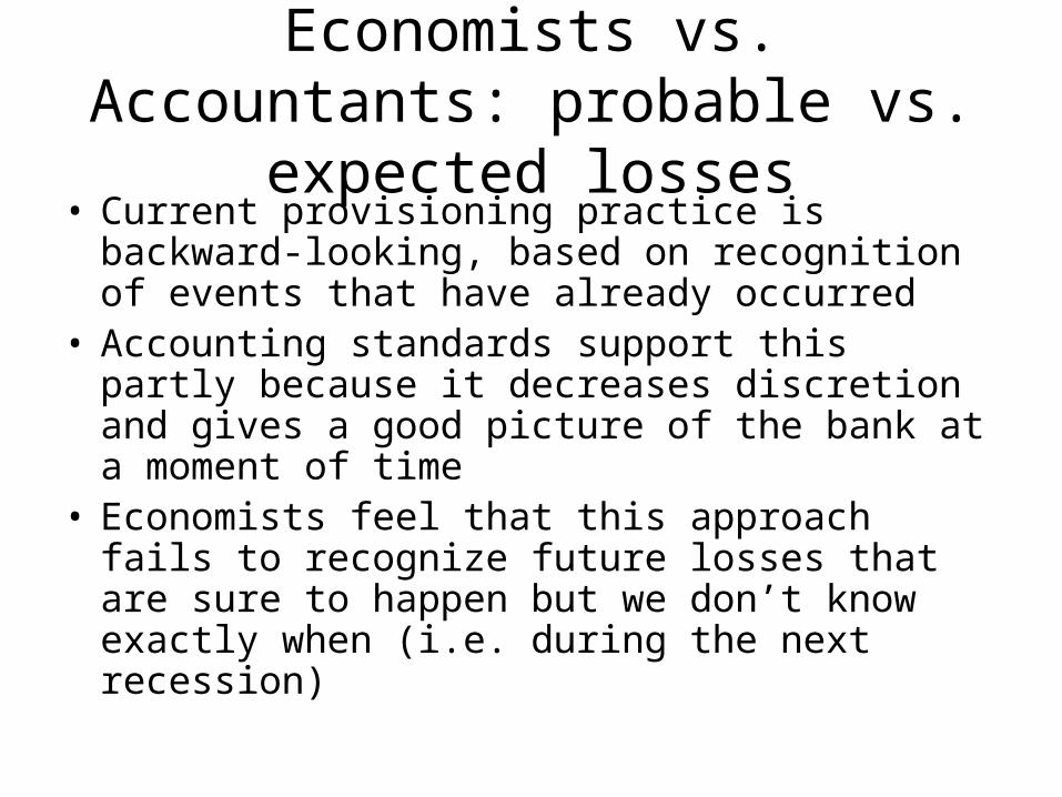
Economists vs. Accountants: probable vs. expected losses

• Current provisioning practice is backward-looking, based on recognition of events that have already occurred

• Accounting standards support this partly because it decreases discretion and gives a good picture of the bank at a moment of time

• Economists feel that this approach fails to recognize future losses that are sure to happen but we don’t know exactly when (i.e. during the next recession)

Provisioning during a recession is not fun

• Harder to raise capital during a recession

• Lower profits or even losses make it painful to create provisions

• Increased provisions are usually seen by markets as a sign of problems and lead to further share price declines

Dynamic provisioning in Spain

• New element: the statistical provision

• A new type of general provision

• Statistical provision based on expected losses for 6 categories of assets

• Provision rates range from 0.1% (loans to firms with grade “A” long-term debt ratings) to 1.5% (current account overdrafts and credit overdrafts)

The Spanish system

• The basis for the statistical provision is the sum of the provisions on each of the six asset categories

• The statistical provision itself is the difference between the bank’s provisions and the standard basis

• Tp = Sp + Gp + St where – Tp is total provisions– Sp is specific provisions– Gp is general provisions– St is the statistical provision

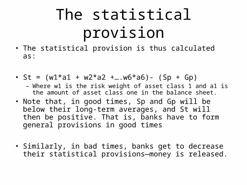
The statistical provision

• The statistical provision is thus calculated as:

• St = (w1*a1 + w2*a2 +….w6*a6)- (Sp + Gp) – Where w1 is the risk weight of asset class 1 and a1 is the

amount of asset class one in the balance sheet.

• Note that, in good times, Sp and Gp will be below their long-term averages, and St will then be positive. That is, banks have to form general provisions in good times

• Similarly, in bad times, banks get to decrease their statistical provisions—money is released.

How the statistical provision “flattens” provisions

Some things to note

• The loss probabilities for different asset classes are based on 16 years worth of data (two business cycles).

• The Spanish system assumes that losses in the next business cycle will be the same on average as in the last business cycle.

• The Spanish system seems to be incompatible with IAS 39.

Can Dynamic provisioning work in Croatia?

• Provisioning does seem to be cyclical…

0

5

10

15

20

25

pro

.96

tra.9

7

kol.97

pro

.97

tra.9

8

kol.98

pro

.98

tra.9

9

kol.99

pro

.99

tra.0

0

kol.00

pro

.00

tra.0

1

kol.01

pro

.01

tra.0

2

kol.02

pro

.02

tra.0

3

(%) max

median

min

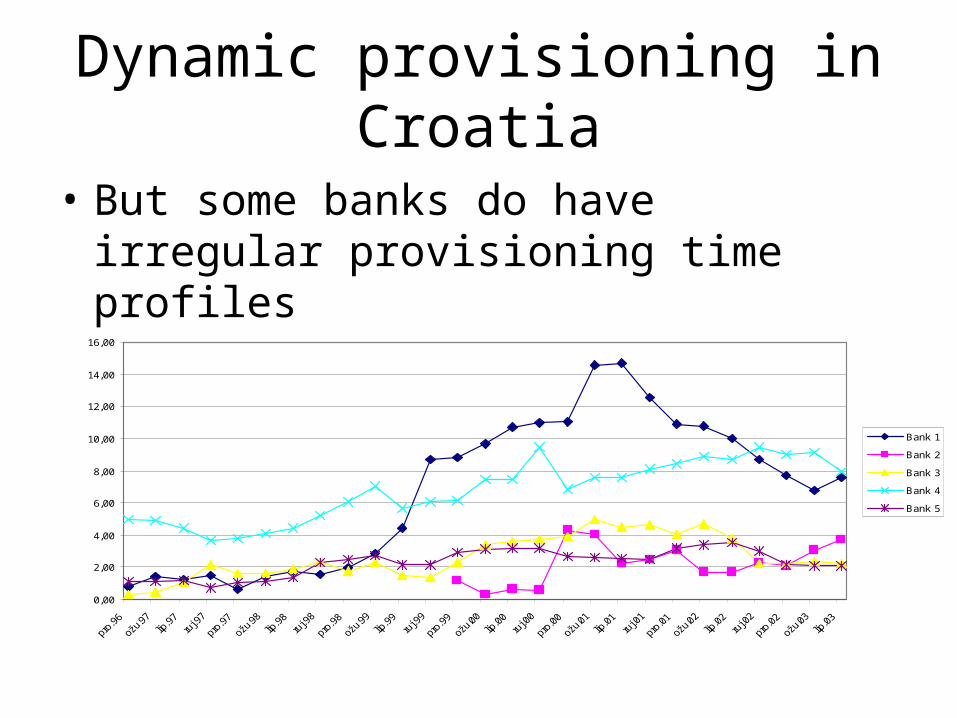
Dynamic provisioning in Croatia

• But some banks do have irregular provisioning time profiles

0,00

2,00

4,00

6,00

8,00

10,00

12,00

14,00

16,00

Bank 1

Bank 2

Bank 3

Bank 4

Bank 5

A first try

• simulation 1: total provision = actual + 0.75 x (4.78 - actual)

– (4.78 is the average for the whole banking system over the whole time period studied)

• simulation 2: total provision = actual + 0.75 x (bank's average Q4 96 to Q2 03 – actual)

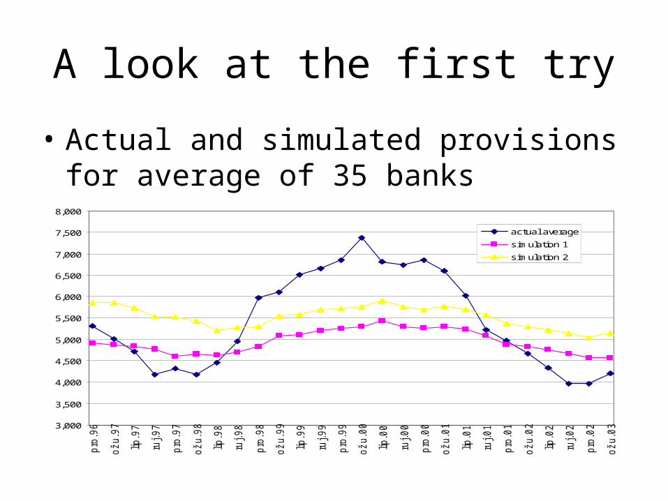
A look at the first try

• Actual and simulated provisions for average of 35 banks

3,000

3,500

4,000

4,500

5,000

5,500

6,000

6,500

7,000

7,500

8,000

pro

.96

ožu.9

7

lip.9

7

ruj.97

pro

.97

ožu.9

8

lip.9

8

ruj.98

pro

.98

ožu.9

9

lip.9

9

ruj.99

pro

.99

ožu.0

0

lip.0

0

ruj.00

pro

.00

ožu.0

1

lip.0

1

ruj.01

pro

.01

ožu.0

2

lip.0

2

ruj.02

pro

.02

ožu.0

3

actual average

simulation 1

simulation 2

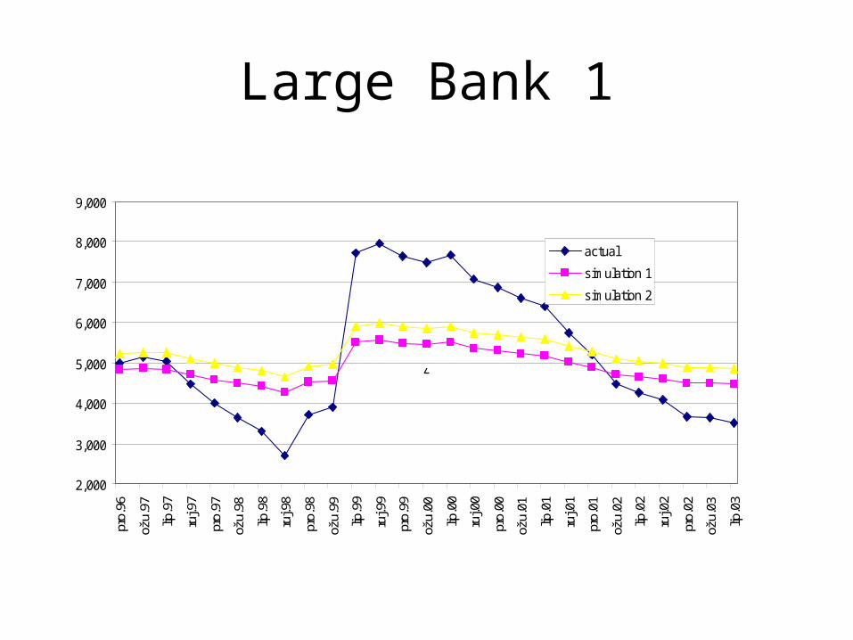
Large Bank 1

2,000

3,000

4,000

5,000

6,000

7,000

8,000

9,000

pro.

96

ožu.

97

lip.9

7

ruj.9

7

pro.

97

ožu.

98

lip.9

8

ruj.9

8

pro.

98

ožu.

99

lip.9

9

ruj.9

9

pro.

99

ožu.

00

lip.0

0

ruj.0

0

pro.

00

ožu.

01

lip.0

1

ruj.0

1

pro.

01

ožu.

02

lip.0

2

ruj.0

2

pro.

02

ožu.

03

lip.0

3

actual

simulation 1

simulation 2

Z

Large Bank 2

3,000

4,000

5,000

6,000

7,000

8,000

9,000

10,000

11,000

12,000

pro.

96

ožu.

97

lip.9

7

ruj.9

7

pro.

97

ožu.

98

lip.9

8

ruj.9

8

pro.

98

ožu.

99

lip.9

9

ruj.9

9

pro.

99

ožu.

00

lip.0

0

ruj.0

0

pro.

00

ožu.

01

lip.0

1

ruj.0

1

pro.

01

ožu.

02

lip.0

2

ruj.0

2

pro.

02

ožu.

03

actual

simulation 1

simulation 2

Large Bank 3

0,000

0,500

1,000

1,500

2,000

2,500

3,000

3,500

4,000

4,500

5,000

pro

.96

ožu.9

7

lip.9

7

ruj.97

pro

.97

ožu.9

8

lip.9

8

ruj.98

pro

.98

ožu.9

9

lip.9

9

ruj.99

pro

.99

ožu.0

0

lip.0

0

ruj.00

pro

.00

ožu.0

1

lip.0

1

ruj.01

pro

.01

ožu.0

2

lip.0

2

ruj.02

pro

.02

ožu.0

3

lip.0

3

actual

simulation 1

simulation 2

Effect on profits

• Large Bank 2

-2,00

-1,00

0,00

1,00

2,00

3,00

4,00

5,00

pro

.96

ožu.9

7

lip.9

7

ruj.97

pro

.97

ožu.9

8

lip.9

8

ruj.98

pro

.98

ožu.9

9

lip.9

9

ruj.99

pro

.99

ožu.0

0

lip.0

0

ruj.00

pro

.00

ožu.0

1

lip.0

1

ruj.01

pro

.01

ožu.0

2

lip.0

2

ruj.02

pro

.02

ožu.0

3

actual ROA

ROA with stat prov

A new approach

• Idea: try to estimate how rapidly the average provision is falling over time, controlling for the business cycle

• Result: provisioning falling 0,06 percentage points per year

Another try

• simulation 3: total provisions= bank fixed effect - 0,061 time

• simulation 4: total provisions= actual - 0,061 time - 2

What it looks like

• Average for all banks

0,000

1,000

2,000

3,000

4,000

5,000

6,000

7,000

8,000

simulation 3

actual

stimulation 4

Is it adequate?

• Requires confidence that future decreases in provisioning will follow at the same pace as past decreases

• Produces negative overall provisions for some banks in some quarters

• Not very simple and probably not too robust

Concluding thoughts

• Dynamic provisioning seems attractive as a way to decrease financial instability

• But it is easiest to implement in stable markets with long data series and stable provisioning levels

• One can either be patient and wait for more data or look at other ways to achieve the same goals.