dynamic multi-contact motions © The Author(s) 2013 multi-contact motions The International Journal of ... satisfaction guaranteed motions for any time grid. ... and dynamic multi-contact

Article

Generation of whole-body optimaldynamic multi-contact motions

The International Journal ofRobotics Research32(9-10) 1104–1119© The Author(s) 2013Reprints and permissions:sagepub.co.uk/journalsPermissions.navDOI: 10.1177/0278364913478990ijr.sagepub.com

Sébastien Lengagne1,2, Joris Vaillant1,3, Eiichi Yoshida1 and Abderrahmane Kheddar1,3

AbstractWe propose a method to plan optimal whole-body dynamic motion in multi-contact non-gaited transitions. Using aB-spline time parameterization for the active joints, we turn the motion-planning problem into a semi-infinite programmingformulation that is solved by nonlinear optimization techniques. Our main contribution lies in producing constraint-satisfaction guaranteed motions for any time grid. Indeed, we use Taylor series expansion to approximate the dynamicand kinematic models over fixed successive time intervals, and transform the problem (constraints and cost functions) intotime polynomials which coefficients are function of the optimization variables. The evaluation of the constraints turns theninto computation of extrema (over each time interval) that are given to the solver. We also account for collisions and self-collisions constraints that have not a closed-form expression over the time. We address the problem of the balance withinthe optimization problem and demonstrate that generating whole-body multi-contact dynamic motion for complex tasks ispossible and can be tractable, although still time consuming. We discuss thoroughly the planning of a sitting motion withthe HRP-2 humanoid robot and assess our method with several other complex scenarios.

KeywordsMulti-contact motions,optimization, balance, Taylor series approximation, time-interval discretization, humanoid robots

1. Introduction

Planning dynamic motion for complex robotic systems suchas humanoids, under various constraints, is known to be acomplex problem in robotic research. For example, loco-motion in cumbersome environments is non-gaited andapproaches developed for biped cyclic locomotion do notapply. We propose a method that can generate gaited ornon-gaited, optimal and dynamic multi-contact motions ofthe robotic system (in the sense of integrating a preview ofwhat the following support contacts are).

Classical approaches usually solve the problem in twosteps: the first step plans the motion of a reduced sim-ple model (Kajita et al., 2003) that encompasses the maininvariants of the motion (center of mass, centers of pressure,etc.); the second step consists of generating the whole-bodydynamic motion that tracks at best the first step plan butwhere additional constraints (joint limits, torque limits, col-lision detection, etc.) are checked a posteriori. Hence, thefirst step assumes viability of the second step. In some typ-ical tasks (e.g. walking) precaution are taken for the firststep planning to generate very likely feasible plans. How-ever, for more general tasks such as moving in cumbersomesituations it is hard to both plan based on reduced/simplemodels and make plausible assumptions on the feasibilityof the plan for the whole-body motion.

In this paper, we solve whole-body planning using non-linear optimization techniques and a full-body dynamicmodel. Optimization techniques were used as early as the1980s in robotic motion planning. The starting point ofour work is the result obtained by Lee et al. (2005); Leeet al. proposed a method to generate motions for robots withredundant or exactly actuated closed chains. This method isbased on the optimization of the parameters of the joint tra-jectories and computes analytically the model of the robotand its derivative. Their algorithm was illustrated with 2Dsimulation examples and we considered whether it is pos-sible to extend the approach for the 3D complex case ofmulti-contact motions for humanoid robots. That is, how toimpose unilateral constraints on the contact forces, ensure

1CNRS-AIST Joint Robotics Laboratory (JRL), UMI3218/CRT, Tsukuba,Japan2Karlsruhe Institute of Technology, Institute for Anthropomatics,Humanoids and Intelligence Systems Lab, Karlsruhe, Germany3CNRS-Université Montpellier 2, LIRMM, Interactive Digital Humangroup, Montpellier, France

Corresponding author:Sébastien Lengagne, Karlsruhe Institute of Technology, Institute forAnthropomatics, Humanoids and Intelligence Systems Lab, Adenauerring2, 76131 Karlsruhe, Germany.Email: [email protected]

Lengagne et al. 1105

balance, include collision avoidance and guarantee con-straint satisfaction not only at sample time but also all alongthe motion whatever time-grid size is chosen? Our presentwork tackles these issues. The work by Lee et al. (2005) iscertainly the root of our approach. However, we proposeseveral novel contributions in order to generate complexand dynamic multi-contact motions for humanoid robots.

In Section 2, we present the related work about motiongeneration for humanoid robots and emphasize the lack ofefficient methods to generate complex and dynamic multi-contact motions. Then, we present the mathematical modelof the robot and the analytical formulation of the con-tact forces in Section 3. Section 4 is about formulatingthe motion generation problem as a nonlinear optimiza-tion. To solve this problem and produce motions with guar-anteed constraint satisfaction all over the time, includingnon-desired collisions avoidance, Section 5 introduces oursecond contribution: the time-interval discretization. Thisdiscretization is based on Taylor series expansion approx-imation for the continuous state variables of the robot.Finally, in Section 6, we discuss the technical details andvalidate our method with several complex scenarios such asa sitting motion for the HRP-2 (Kaneko et al., 2004), whereboth hands, both feet and the waist are involved in contacttransitions during motion.

2. Related work

Previous work proposed several approaches in order togenerate sequences of contact stances, to compute opti-mal motions, to characterize its balance and to performexperiments of multi-contact motions.

Recently, there is an increasing interest in planning non-gaited motion where a humanoid robot is allowed to con-tact the environment with any possible part of its body tosupport motions in bulky and uneven spaces. For exam-ple, Bouyarmane et al. (2009); Bouyarmane and Kheddar(2012), Escande and Kheddar (2009); Escande et al. (2006),and Hauser et al. (2005); Hauser and Latombe (2010)developed a contact-before-motion planning algorithm toplan the sequence of contacts for such problems. Complexexamples were illustrated on the HRP-2 robot (Escandeand Kheddar, 2009; Escande et al., 2008). However, inthese experiments, the motion between successive contacts,namely the transitions, was not fully dynamic. Our presentcontribution aims at filling this gap. That is, generatingoptimal dynamic motions in multi-contact transitions.

Optimal control methods are used to generate (periodic)complex motions such as one-legged hopping, walking(Mombaur et al., 2005) and running (Schultz and Mom-baur, 2010). They are usually categorized into three dif-ferent types (Diehl et al., 2006): (i) dynamic programmingmethods are based on the principle that the optimality ofsub-arcs is restricted to small state dimensions; (ii) indi-rect methods use the Pontryagin’s maximum principle, buthave a small domain of convergence; (iii) direct methods

that transform the infinite problem into a finite nonlinearprogramming problem (NLP) are commonly used for realsystems such as humanoid robots.

The direct methods are composed of the direct singleshooting, collocation and direct multiple shooting methodsfor which the control and/or the state variables are dis-cretized and use the direct dynamic model of the robot. Afourth direct method uses parameterization. It finds a localsolution of the optimal control through optimal values ofthe trajectories’ parameters; as an example of parameteri-zation B-splines are widely used, (cf. Lee et al.(2005) andMiossec et al. (2006)). Parameterization proved to be par-ticularly efficient in robotics (Steinbach, 1997; von Stryk,1998). In this case, an inverse dynamic model can beused that allows the motion to be decomposed into sev-eral independent parts, which can be parallelized usingmulti-thread software. Using state-of-the-art parameteriza-tion based methods, continuous time-dependent constraintsare still discretized into a finite set of discrete constraintsover a time grid. This kind of method was used by Arisumiet al. (2008) to realize the lifting motion of 23.4 kg withthe HRP-2 humanoid (Kaneko et al., 2004). Each time anexperiment crashed during trials, investigation of log datarevealed that the torque constraint was violated in betweentwo points of the chosen time grid, albeit the optimizationprocess ended successfully. In that sense, this method isnot safe, since the user cannot trust the results of the opti-mization process. At that time, the optimization problemwas reformulated with smaller time grid, recomputed andre-experimented until success.

This observation motivates the work we performed andpresent here. Our new formulation, guarantees that, undermodel-match hypothesis, in the case of successful termina-tion of the optimization process, the planned motion willnot violate any constraints all along the time motion what-ever discretization range is. This is the reason why we call itsafe. One can use the time-interval discretization proposedby Lengagne et al. (2011c) but at the price of a substan-tially much longer computation time. We can also proceedin a recursive way by running the optimization using a timegrid, and then compute the violation of the constraints usingthe time interval while penalizing the bounds of the con-straints until no violation occurs as presented by Lengagneet al. (2011c). Yet, those methods cannot deal with continu-ous equality constraints that describe the constant positionof a body during a contact stance.

Specific to humanoids robots, balance is a very chal-lenging and a difficult issue. During walking motions, thebalance of the robot is usually characterized by the zeromoment point (ZMP) (Vukobratovic and Borovac, 2004).Unfortunately, the use of the ZMP assumes that there areonly co-planar contacts and cannot apply to general multi-contact motions. One can also consider the generalizedZMP (GZMP) (Harada et al., 2006) or the foot rotationindex (Goswami, 1999). To characterize the balance of therobot, we rather monitor whether the contact wrench sum

1106 The International Journal of Robotics Research 32(9-10)

Fig. 1. Description of the contact of the left hand with the table.The frame Xi is linked to the body and must coincide the expectedframe Xe

i on the table.

(CWS), due to gravity and dynamic effects, remains in thecontact wrench cone (CWC) as presented by Hirukawa et al.(2006). From this definition of the balance, we propose ananalytical formulation of the contact forces.

The use of reduced models during the optimization canlead to some constraints violation a posteriori. We bet-ter plan the motion with the most complete model andconstraints possible in order to guarantee that whole-bodymotion is highly likely feasible. The choice of the full-bodymodel impacts on the complexity of the computation, andhence on the computation time; but is the only way to ensurea priori a viable plan of the robot.

Collisions with the environment and the self-collisionsare also critical constraints to handle during motion plan-ning. However, collision avoidance requires the evaluationof the distance to obstacle. In order to have good perfor-mances of the optimization process, it is highly suggested toconsider convex bounding shapes to describe the bodies ofthe robot such as the Sphere-Torus-Patch Bounding Volume(STP-BV) presented by Escande et al. (2007). This solutionallows us to have continuous gradient of the distances andwe are using it in our problem formulation. To ensure thecollision avoidance over the entire motion’s duration, somemethods such as the continuous collision detection (Zhanget al., 2007) use Taylor models and temporal culling.

We assume a perfect full-body dynamic rigid model ofthe HRP-2 robot and a perfect knowledge of its environ-ment. However, to perform real experiments, the last issueis subject to the control approach of the robot during multi-contact stances. Work by Hyon et al. (2007) and Stephensand Atkeson (2010) proposed a balance controller based

on the control of the forces, whereas the work of Lee andGoswami (2012) was based on the control of both linearand angular momentum of the robot. Interestingly Sentiset al. (2010) presented a methodology to control the inter-nal forces and center of mass (COM) during a multi-contactinteraction between a humanoid robot and the environmentusing a virtual linkage model. This method was validated insimulations of manipulation tasks without locomotion, suchas cleaning a board or manipulating a panel. Eventually, acontroller used during locomotion of robots is presented by(Righetti et al., 2011); it uses the redundancy of the multi-contact motion to create optimal distribution of the contactforce and was successfully applied to a quadruped robotduring actual experiments. In our work, we assume thatthe robot’s controller tracks the generated joint trajectoriesperfectly under little model uncertainties.

3. Multi-contact motion definition

In this section, we present the model and the constraints thatare needed to generate a multi-contact motion.

3.1. Kinematics

First, we deal with the kinematic constraints. A contactis defined simply as the relative configuration of a givenrobot’s link regarding the environment, excluding sliding.This can be defined with equality constraints involving twoCartesian frames: one on the contact body Xi and the otherone on the environment at the expected desired positionof the contact Xe

i (Figure 1), where X ∈ R6 denotes the

six-component contact vector of a frame position and ori-entation (X = [x, y, z, θx, θy, θz]T). In order to consider Nc

contacts during a time interval [�t], we must ensure a setof ni continuous equality constraint for each contacts asfollows:

∀t ∈ [�t], ∀i ∈ {1, . . . , Nc}, ∀j ∈ {1, . . . , ni}kini,j( Xi( t) , Xe

i ) = 0 (3.1)

where ni is the number of constraints for each type of con-tact. For a planar rigid contact there are three rotations andthree positions constraints (ni = 6). The general formu-lation of Equation 3.1 allows to consider planar, edge orpoint contacts. Moreover, we consider fully and partiallydefined contacts: the value of some components of the con-tact position and/or orientation can be unknown (but muststay constant). For example, for a planar rigid contact, oneconsiders

∀t ∈ [�t], ∀i ∈ {1, . . . , Nc}, ∀j ∈ {1, . . . , 6}{if κi,j = 1 → Xi,j( t) = Xe

i,j

if κi,j = 0 → ddt Xi,j( t) = 0

(3.2)

where κi,j is a Boolean attached to the jth component ofthe ith contact vector. This Boolean is equal to one if thecomponent value is known and is equal to zero if the com-ponent value is unknown, in the case of partially defined


contacts. In the latter case, the actual value will be a resultof the optimization process. Equations (3.1) will imposethe kinematic behavior of the motion. The balance of themotion will depend on the dynamic of the motion as definedhereafter.

3.2. Inverse dynamic model

We plan motion with the full-body dynamic model of thehumanoid robot:[

�

0

]=[

M1( q)M2( q)

]q +

[H1( q, q)H2( q, q)

]+[

JT1 ( q)

JT2 ( q)

]F

(3.3)where q( t) ∈ R

Ndof is a vector containing the Ndof joint posi-tion ( qi( t) , �( t)) , ∈ R

Ndof is the vector of the joint torques,F( t) is the vector of the Nf active linear contact forces,M1 ∈ R

Ndof ×Ndof and M2 ∈ R6×Ndof are the two compo-

nents of the inertial matrix, H1 ∈ RNdof and H2 ∈ R

6 thetwo components of vector due to gravity, centrifugal andCoriolis effects, J1 ∈ R

Ndof ×3Nf and J2 ∈ R6×3Nf are the

components of the Jacobian matrix. Equation (3.3) assumesthat the first contact (from which the waist trajectory is com-puted, see Lengagne et al. (2010b)) is always maintained.This assumption is enforced by adding constraints on thebalance of the robot as presented in Section 3.6. Equa-tion (3.3) emphasizes the link between the contact forcesand the joint torques. To know the joint torques, it is nec-essary to know the joint trajectories and the contact forces.Regarding the known joint trajectories, there is an infiniteset of combination joint torques–contact forces, depend-ing on the internal forces. In the following, we present ourmethod to get rid of this indetermination and compute thejoint torques and contact forces from the joint trajectoriesand a few additional variables, in a way that enforces thebalance of the robot.

3.3. Balance

To characterize the balance of the motion, we constrain theCWS, due to gravity and dynamic effects, to remain withinthe CWC as presented by Hirukawa et al. (2006). In fact, weensure that the contact forces that counterparts the dynamiceffect D2 = M2( q) q+H2( q, q) must be feasible, i.e. hold adesired contact state, prohibiting from any undesired slidingof the link on the surface or contact removal.

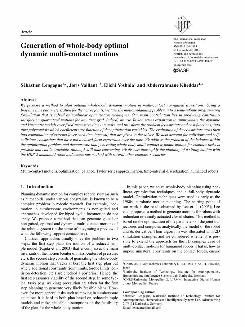
We define a set of Nf linear forces F = {F1, F2, . . . , FNf }(Fi ∈ R

3), for all of the contacting bodies, as presentedin Figure 2 and their normal and tangent spaces. To avoidunexpected sliding or taking-off of any part of the robot,each linear contact force Fi must fulfill

∀t ∈ [�t], ∀i ∈ {1, . . . , Nf }{

Fni ( t) > 0

||Fti ( t)||2 ≤ μ2

i Fni ( t)2

(3.4)where Fn

i is the normal component of the contact force, Fti

is the 2D vector of the tangent force and μi is the friction

Fig. 2. Description of the contact forces for the left foot. Weconsider four forces: one for each corner of the foot sole.

coefficient at contact i. For each contact forces i, those twoconstraints can be merge into the equivalent equation:

fric( Fi( t) ) = Fi,x( t)2 + Fi,y( t)2 − sign( Fi,z)

× μ2i Fi,z( t)2 ≤ 0 (3.5)

Note that we consider the z-axis as the normal axis at thecontact space. Moreover, those contact forces must be coun-terparts to the dynamic effect by satisfying the second partof the dynamic Equation (3.3), that is

D2( q, q, q) +JT2 ( q) F = 0 (3.6)

3.4. Contact forces

In our previous work (Lengagne et al., 2010b), a 2D-modelstudy of this problem revealed that Equation (3.6) cannotbe satisfied if the contact forces are parameterized usingB-spline functions. Hence, we compute the value of the con-tact forces F = {F1, F2, . . . , FNf } from the joint trajectoriesthat exactly counterpart the dynamics effects while fulfill-ing the constraint of Equation (3.4) as best as possible, i.e.the contact forces that solve

min 12

∑i βi( αi||Ft

i ||2 + Fni

2)

D2( q, q, q) +JT2 ( q) F = 0

(3.7)

where Fni is the normal component of the contact force Fi;

Fti the 2D vector component of the tangent component of

the contact force Fi; βi and αi are weight coefficients asdetailed in Appendix A. The exact satisfaction of these con-straints is left to the optimization solver. Appendix A shows


how to obtain the analytical formulation of the contactforces such as

Fi = W−1i

[PiAi Ai

]�−1

D2 (3.8)

with

� =∑

i

([PiAi

Ai

]W

−1i

[PiAi Ai

])(3.9)

and where:

• Wi = diag( βiαi, βiαi, βi) is a weight matrix;• βi > 0 weights the contact forces i regarding the other

forces;• αi � 1 weights the tangential components regarding the

tangential ones;• Pi, Ai are the position and orientation of the contact

forces.

The matrix � is a 6 × 6 matrix that we invert usingthe Gauss–Jordan algorithm, to compute the value of thecontact forces F.

3.5. Collision avoidance

During multi-contact motion transitions, there are parts ofthe robot for which we seek a sustained collision with theenvironment (desired motion supporting contacts), and theremaining part that should avoid (non-desired) collisions.Therefore, planning motion considers collision avoidanceas a constraint. Let Li be the ith link of the robot, i ∈ [1, Nl]for a robot having Nl identified links or all of the sub-partthat are convex composing all links, and let Oi be a setobstacles among No ones. Avoiding collision can be simplywritten as

d(Li,Oj) ( t) ≥ ε (3.10)

where d( X , Y ) ( t) is the distance separating body X frombody Y , the pair i, j is the list of the defined links/obstaclesto be checked and ε is a security margin. This constraintmeans that the separating distance between two any bodymust be kept positive (at ε margin) all along the motion.Self-collisions are enforced similarly:

d(Li,Lj) ( t) ≥ ε i �= j and j �= i − 1 (3.11)

There are several methods to compute the distanceamong pairs of geometrical objects. The simple the geom-etry the faster is the computation. This is the reason whyin robotics we use bounding volume for the links (e.g. cap-sules, oriented bounding boxes, etc.). Since we are usingthe distance in the frame of an optimization problem, manysolvers require computing the gradients of the constraints.In order to fulfill existence and continuity of the distancefunction gradients, while keeping fast computation, weneed to have strictly convex bounding volume of the links.We devised in our previous papers such new bounding vol-ume operator, called STP-BV that achieved bulged convex

hulls so as the distance computation is fast and its gradi-ent C1 continuous (Escande et al., 2007; Benallegue et al.,2009). Note that computing the distance δ is the outcome ofa local optimization process.

3.6. Constraints

We define a multi-contact motion by a sequence of multi-contact phases. One phase is an amount of time for whichall the contacts hold (no creation or release of contacts).The transition between two phases is done when at least onecontact is created or released.

The generation of the multi-contact motions is equiva-lent to finding the joint trajectories, the contact forces andthe duration over each contact phase. This motion must val-idate a set of equality (Equation (3.12a)) and inequality(Equations (3.12b)–(3.12f)) continuous constraints:

∀t ∈ [�t], ∀i ∈ {1, . . . , Nc}, ∀j ∈ {1, . . . , ni}kini,j( Xi( t) , Xe

i ) = 0 (3.12a)

∀t ∈ [0, T], ∀i ∈ {1, . . . , Ndof } qj≤ qj( t) ≤ qj

(3.12b)∀t ∈ [0, T], ∀i ∈ {1, . . . , Ndof } qj ≤ qj( t) ≤ qj

(3.12c)∀t ∈ [0, T], ∀i ∈ {1, . . . , Ndof } �j ≤ �j( t) ≤ �j

(3.12d)∀t ∈ [0, T], ∀i ∈ {1, . . . , Nf } fric( Fi( t) ) ≤ 0

(3.12e)∀t ∈ [0, T], ∀i ∈ {1, · · · , Nd} δi ≥ ε (3.12f)

where δi = sign( di) d2i is the signed square distance

between two bodies, this value is returned by the algorithmpresented by Benallegue et al. (2009). One can also con-sider a set of k discrete constraints on any state xk of therobot in order to specify desired property of the motion.

∀k, zk( xk , tk) ≤ 0 (3.13)

4. Problem formulation

In the previous section, we detailed the model and the con-straints of a multi-contact motion. Now, we introduce thebasics in terms of terminology, notation, and the generalformulation of the nonlinear optimization problem.

4.1. Motion planning problem

The motion generation process solves the following opti-mization problem:

minq(t),�(t),F(t),Tf

C( q( t) , q( t) , q( t) , �( t) , F, Tf )

subject to{�, F} = IDM( q, q, q)

ceq( q, q, q, �, F) = 0cineq( q, q, q, �, F) ≤ 0

cteq( q( td) , q( td) , q( td) , �( td) , F( td) ) ≤ 0

(4.1)


This formalism is used by Miossec et al. (2006). Usually,the constraint {�, F} = IDM( q, q, q) is replaced by thedirect dynamic model x( t) = f ( x( t) , u( t) ) where x( t) isthe state variable and u( t) the control variables (Schultzand Mombaur, 2010), but both representations are math-ematically equivalent and differ only from the implemen-tation viewpoint. Thus, the optimal control problem (4.1)can be considered as an infinite programming (IP) problemthat consists of finding the joint trajectories q( t), the forcecoefficient β and the phase durations Tf :

argminq(t),β,Tf

C( q( t) , β, Tf )

∀i, ∀t ∈ [�i] gi( q( t) , β, Tf ) ≤ 0∀j, ∀t ∈ [�j hj( q( t) , β, Tf ) = 0∀tk ∈ {t1, t2, . . .} zk( q( tk) , β, Tf ) ≤ 0

(4.2)

where C is the cost function, which accounts for quanti-tative and/or qualitative robot motion in given applicationcontexts. Well-known cost functions in robotics are: motionduration (Piazzi and Visioli, 1998; Bobrow, 1988), mini-mum torque (Breteler et al., 2001), global energy consump-tion (Miossec et al., 2006), jerk for smooth motion (Piazziand Visioli, 2000), torque change (Uno et al., 1989), or anyweighted combination of the above and more. In the equa-tion, g, h and z are, respectively, the continuous inequal-ity and equality and the discrete inequality constraints aspresented in Section 3.6.

We voluntary omit the discrete constraints z, since theydo not lead to any kind of problem in the state-of-the-artmethods.

4.2. Semi-infinite programming

The problem (4.2) is an IP since the solution to be found isa set of continuous functions q( t) that fulfill a set of con-tinuous constraints all along the time t (both can be seenas infinite sets of discrete values). In order to make an IPcomputationally solvable, most of the methods (Reemtsenand Rückmann, 1998) reduce such complexity by defininga parameters set P ∈ R

N that gives at least a parametricshape for the functions to be found (the optimal trajectoriesq( t)):

q( t) = f ( P, t) (4.3)

Based on prior work in robotics (e.g. Lee et al., 2005), wechose to shape the joint trajectories with clamped uniformcubic B-spline curves. A B-spline function is the weightedsum of k-order basis functions defined by m number ofcontrol points:

∀t ∈ [�t] q( t) =m∑

i=1

bki ( t) pi (4.4)

The basis functions bki ( t) are computed using the Cox–de

Boor recursion (de Boor, 1978) and the control points ρi arepart of the parameters of the motion. This parameterizationwas already used for motion generation by Lee et al. (2005)

and Miossec et al. (2006). Subsequently, the motion plan-ning problem turns to finding the best parameter set P ∈ R

N

such asargmin

PC( P)

∀i, ∀t ∈ [�i] gi( P, t) ≤ 0∀j, ∀t ∈ [�j] hj( P, t) = 0

(4.5)

This problem is a semi-infinite programming (SIP) (Reemt-sen and Rückmann, 1998) since it deals with a finite setof optimization variables P ∈ R

N , which must satisfy aset of continuous constraints. The detail of the optimizationparameter vector P in our case in presented in Section 6.1.

5. Dealing with continuous constraints

Enforcing joint position and velocity limits is straightfor-ward, see Appendix B. For more complex constraints suchas torques, we use a time-interval discretization based on apolynomial approximation.

5.1. Time-interval discretization

Most of the solvers cannot deal with continuous constraintsand require a finite number of constraints. Although thetime-grid discretization is widely used (Hettich and Kor-tanek, 1993; Reemtsen and Rückmann, 1998; von Stryk,1993), it assumes (but does not guarantee) that if a con-straint holds at times tk and tk+1, then it holds ∀t ∈ [tk , tk+1](Lengagne et al., 2011c). We experienced in our previousattempts (Arisumi et al., 2008; Lengagne et al., 2011c)and highlight that violations of the limits may happen,even when the optimization algorithm ended with suc-cess status. To solve this issue and generate motions in asafe way, the time-interval discretization (Lengagne et al.,2011c) replaces the continuous inequality constraints of theoptimization problem by

∀i, ∀[t] ∈ IT sup( [g]i( P, [t]) ) ≤ 0 (5.1)

where IT = {[t]1, [t]2, · · · , [t]q−1, [t]q} and [t]n = [tn−1, tn]is the time interval decomposition of the phase �t. In ourprevious work (Lengagne et al., 2011c), we computed aconservative value of the extrema over each time inter-val [t]i, and the optimization solver can produce a motionthat guarantees all of the constraint validity over the entiremotion duration. Unfortunately, this method has a hugecomputation time. In this paper, we consider the same time-interval discretization, but we rather use Taylor approxima-tion, which reduces the computation time substantially andallows us to deal with continuous inequality and equalityconstraints.

5.2. Taylor approximation

5.2.1. Principle In order to perform a time-interval dis-cretization (Equation (5.1)) that considers continuousinequality and equality constraints, we use a polynomial


Taylor approximation of the constraints. Taylor expansionwas also used by Zhang et al. (2007) to tie the bounds ofthe bounding box hierarchies for collision detection.

The original computations (Lengagne et al., 2011c),based on interval analysis, do not keep track of the correla-tion between the different sub-functions which leads to anoverestimation of the bounds (Zhang et al., 2007). To over-come this drawback, we define each function over a timeinterval �t = [ts, te] as a n-order polynomial function:

∀t ∈ [�t] f ( t) =n∑

i=0

ai( P) ×ti (5.2)

where n is the order of the approximation, {a0(P),a1(P) , . . . , an(P) } ∈ R

n+1 are the coefficient of the poly-nomial depending on the optimization parameters P. Com-pared with previous work (Berz et al., 1998), we voluntaryomit to compute the remaining error interval [ε], assumingthat we choose the order n of the polynomial approximationso that we can neglect it (Lengagne et al., 2010a).

5.2.2. Inequality Since we get a polynomial function ofthe constraints (cf. Equation (5.2)), we want to know theextrema of this polynomial over the considered among oftime [�t]. Some work approximate the extrema of a polyno-mial based on the Inequality of the Means (de Alwis, 2004),but cannot find it for a given interval. Several methods findthe extrema based on polynomial root finding of the deriva-tives of the original polynomial. Analytical approaches failfor polynomial having an order n > 5. In order to evalu-ate this extrema for any order n, we use the property of theB-splines explained in Appendix B. That is, given a polyno-mial, the function f ( t), and hence its extrema, are containedwithin the convex hull of the equivalent control points ρi.Therefore, we obtain

∀t ∈ [�t], f ≤ f (t) ≤ f =⇒ ∀i, f ≤ ρi ≤ f (5.3)

with

[ρ0, ρ1, . . . , ρn] = [a0, a1, . . . , an] × B−1 (5.4)

and where B ∈ R(n+1)×(n+1) is a square matrix of the poly-

nomial parameters of the n-order B-spline basis functions1

bni ( t) and relies on the time interval [�t]. Using a time-

scaled implementation of the polynomial, we can computethe inverse B−1 only once and use it all along the opti-mization process. As for the polynomial coefficient, theequivalent B-spline control point ρi rely on the optimizationparameter: ρi( P). Eventually, constraining the equivalentcontrol point ρi to remain within two bounds enforces thecontinuous function to stay within those bounds.

5.2.3. Equality As shown in Section 3.6, multi-contactmotions involve equality constraints that must hold allalong the motion, or at some time intervals in order todefine fully or partially the contacts. These constraints are

the hj( P, t) in Equation (4.5). Using Taylor approximationsof hj, we end up with the polynomial of Equation (5.2) andimpose the coefficients ai( P) to fulfill the constraint

∀i ∈ {0, . . . , Ne} ai( P) = 0 (5.5)

The continuous equality constraint being of order Ne, Ne ≤n is the order that we set for the solver to avoid an over-constrained formulation. As a result, the equality con-straint is fulfilled only under small variation tolerance. Thecompromise between the precision and the optimizationconvergence rate is tuned heuristically with the choice ofNe = 2. Actually, this highlights a deeper fundamentalproblem linked to the choice of the joint trajectory parame-terization for closed kinematics chains. There is certainly avenue for a deeper study specific to this issue.

5.3. Evaluation of collision avoidanceconstraints

We need to compute the minimum of the distance constraintfor a range of time intervals (e.g. for t ∈ [tk , tk+1]). In con-trast to the other constraints, the distance function does nothave a closed-form formula nor an approximate one thatallows it to be written as a polynomial in terms of theoptimization variables. We therefore need to approach theevaluation of mint∈[tk ,tk+1] δ( t) with a numerical method.

In our recent work (Lee et al., 2012), we devised a fastmethod, which evaluates the min distance along a giventime interval. It combines the well-known Golden searchmethod with the conservative advancement technique usedin computer graphics simulation to find the first time of col-lision (see more details in Lee et al. (2012)). Yet, in Leeet al. (2012), we used capsules as bounding volume: notonly they make fast computation of the distance, but thecapsule shape formula allows fast computation of the con-servative advancement bounds. However, the capsule is nota strictly convex shape. In this work, since we use the STP-BV bounding volume, we applied only the Golden searchmethod to seek for the min value of the distance functionon a given time interval with a posteriori check.

6. Experimental validation

6.1. Description of the motion

We validated our method by generating a sitting motionfor the humanoid robot HRP-2 (Kaneko et al., 2004). Thismotion alternates contacts with both hands and feet tofinally contact the waist of the robot with the chair, see Fig-ure 4. The contact of the feet and of the waist are fullydefined by their position and orientation on the ground,whereas the contact of the hand are partially defined, i.e.the hands are asked to contact the table whatever the exactposition.

This motion was decomposed into 13 phases that startfrom the half-sitting motion and end when the robot has


both feet contacting the floor, the left hand contacting thetable and the waist contacting the chair. Each phase isdecomposed into six time intervals and involves nine con-trol points per joints as illustrated on Figure 3. We ensurejoint trajectory continuity by computing the three first con-trol points of the next phase from the three last ones ofthe current phases. Hence, the Cartesian trajectories arecontinuous having smooth transitions between the contactphases.2

For one contacting body over every contact phase, weconsider the same linear evolution of the coefficient β forall of its contact forces. We do not impose the continuityof the coefficient β over the whole motion duration. We set∀i, αi = 1000, this allows us to avoid redundant and unnec-essary optimization parameters. Eventually, the parametervector P ∈ R

n contains all of the control points, the linearcoefficient of β and the phase durations.

During the sitting motion, the degrees of freedom of thehead and of the wrists are set to a constant value, since theydo not impact significantly the balance of the robot. Owingto the fragility of the forces sensor at the endpoints of thearms, we choose to contact the table with the wrist of therobot. We consider seventy different collisions (36 betweenthe robot and its environment and 34 self-collisions). Wealso consider the constraints of the contact forces, the veloc-ity and torque limits (the joint position limits are set bylimits on the variables).

We are considering the following cost function C asthe weighted sum of joint torques, joint jerks and motionduration, as presented:

C( q) = a

∫ T

0

∑i

�2i dt + b

∫ T

0

∑i

...q i

2 dt + cT (6.1)

where a = 1e − 2, b = 1e − 5 and c = 4 are the value weset heuristically to have human-like walking motions withthe HRP-2 (Lengagne et al., 2011a). We choose the ordern = 5 for the polynomial approximation of the constraints.Eventually, the optimization gets 2,339 variables (1,883 freeplus 556 constant variables) and 33,852 constraints.

6.2. Technical implementation

Our method was programmed in the C++ language andexecuted on the following hardware and software: CPUIntel(R) Xeon(R) E5620, 8 cores, 2.4 GHz, Cache 12 Mo:Linux Gentoo 3.0.6 64 bits.

We do not use the Lagrangian formalism of the IDM ofEquation (3.3), but rather use a recursive formulation asin Lee et al. (2005); Park et al. (1995), which is fast andrequires fewer operations (Khalil and Dombre, 2002).

Our software uses template classes for the model andspecialized types to compute the derivative (Bendtsen andStauning, 1996) and the Taylor form of the constraintsand cost functions. The model computation needs a lotof creation and destruction of those types, which induces

many memory allocations. To lower the memory alloca-tions, we use the TC-Malloc library that gives better mallocperformance than the glibc library.

Regarding the optimization solver, we believe3 that it isbetter to use off-the-shelf available solvers since the opti-mization theory provides the fundamentals, but optimiza-tion is also a matter of tricks and recipes of tuning andnumerical robustness. We also apply this policy by using theIPOPT solver (Wächter and Biegler, 2006). IPOPT is free; ithandles large nonlinear optimization problems; it has a C++interface, and was used in (Miossec et al., 2006; Lengagneet al., 2011c).

6.3. Experimental validation

The sequence of the contacts is the output of the methodpresented by Bouyarmane and Kheddar (2012), and is givenas an input to our motion generation method. However,we formulate our problem to allow adjusting these con-tacts. Not all collisions and self-collisions are relevant tocheck and only pertinent ones are accounted for a givenmulti-contact motion problem. We performed several opti-mizations, in order to define the appropriate collisions andself-collisions that deserve to be considered. Often, firstsolutions are not achieved by the robot because they are toofast or result in high impacts or simply too risky to try. Inthese cases we add artificial constraints to drive the solutionto our desired behavior or tune the weights of the cost func-tion. The final collision-free optimization process spent 610iterations and 3h 26mn 37s of computation time to generatethe optimal motion on the entire sequence of contacts, i.e.the entire sitting motion starting from the initial posture tothe final one.

Any experimental validations of this motion is success-fully performed by the HRP-2 robot without exceeding itsphysical limits, without any unexpected collision or self-collisions and keeping its balance, see Figure 4 and Exten-sion 1. The records of the time history of the feet contactforces and joint knee torques are given in Figures 5 and 6.Moreover, this experiment proved to be repeatable at willsince it is often reproduced during VIP visits to our lab.

The cost function and the constraints are model-based.However, the ankle of the robot is equipped with a shockabsorbing mechanism, which is equivalent to having a non-controllable flexible joint. This non-modeled flexible partproduces small hopping of the foot at the beginning ofthe contacting phase. We think that this flexibility is alsothe cause of the release of the contact between the lefthand and the table at the end of the motion (cf. Exten-sion 1). Although we use only local joint PD control, with-out attitude or torque feedbacks, the motion was achievedwith good balance within the physical limits of the robot.Yet, because of the existing discrepancies (e.g. we do notinclude flexibilities in the dynamic model, we might havedifferent friction coefficients at contact, presence of smallunexpected perturbations, etc.) joint torques differ from


Fig. 3. Illustration of the decomposition of the motion into several phases and time intervals. At each time instant the joint trajectoryrelies only on four parameters.

Fig. 4. Experimental validation of the sitting motion.

-100

0

100

200

300

400

500

600

700

0 2 4 6 8 10 12 14

Nor

mal

con

tact

forc

e (N

)

time (s)

experimentoptimization

(a)

-100

0

100

200

300

400

500

600

700

800

0 2 4 6 8 10 12 14

Nor

mal

con

tact

forc

e (N

)

time (s)


(b)

Fig. 5. Experimental validation of the sitting motion, plots of the feet contact forces: (a) left foot; (b) right foot.

the model-computed ones in the planning process; see, forexample, the computed and actual torques of the knees in

Figure 6. Despite this, contact forces shown in Figure 5are quite similar to the computed ones, and this makes


-200

-150

-100

-50

0

50

100

0 2 4 6 8 10 12 14

Nor

mal

con

tact

forc

e (N

)

time (s)


(a)

-120

-100

-80

-60

-40

-20

0

20

40

60

0 2 4 6 8 10 12 14

Nor

mal

con

tact

forc

e (N

)

time (s)


(b)

Fig. 6. Experimental validation of the sitting motion, plots of the knee-joint torques: (a) left foot; (b) right foot.

it possible to identify the contact and non-contact phases.Indeed, as far as the model used in the optimization doesnot differ much, induced errors can still be absorbed bythe PD tracking controller. However, for considerable per-turbations, discrepancies or uncertainties, re-planning isunavoidable.

In general, it does not make sense to include an error-tracking controller as part of the model-base optimizationprocess. However, we need to distinguish between the low-level controller (that is based only on error tracking, whichis assumed null in simulation, since no perturbation) andthe controller strategy that may use robot states or contactforces, etc. A control strategy must be part of the modelwhereas the error tracking controller not.

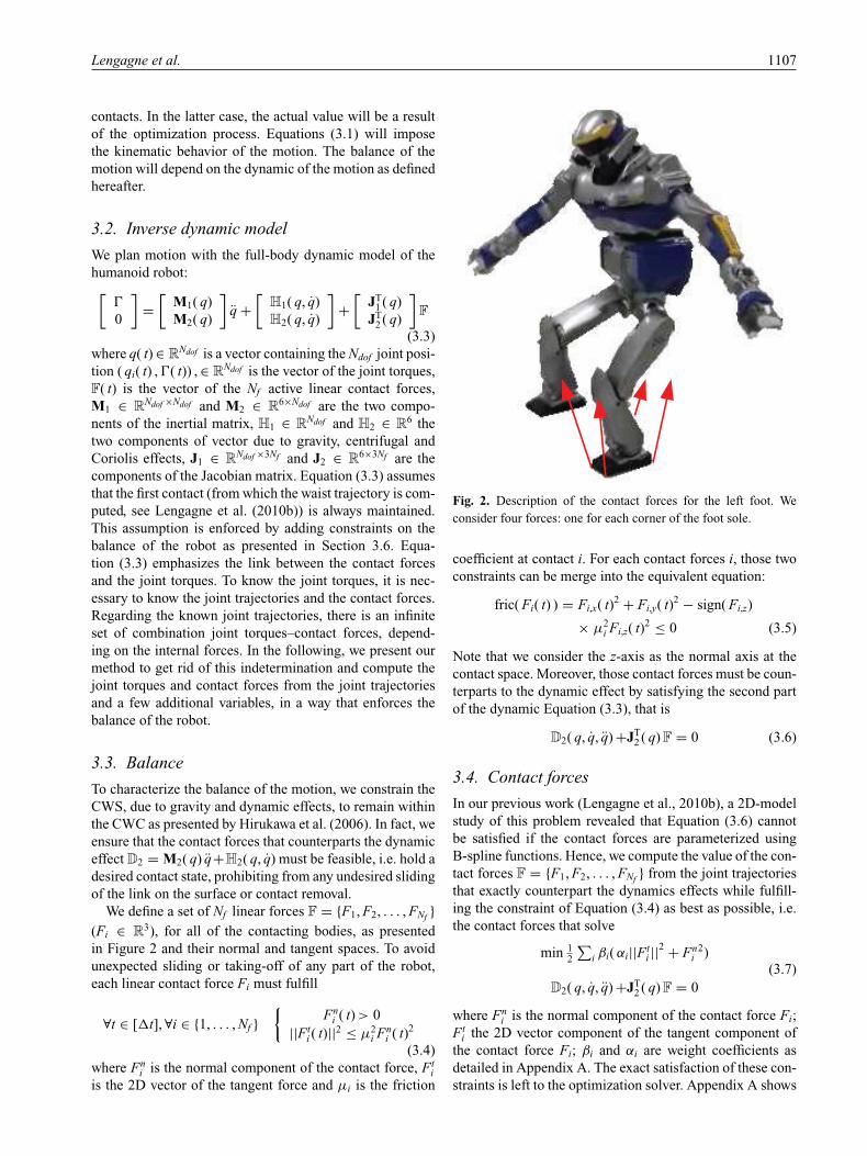
In Figure 7, we present the evaluation of the constraintfor the collision and self-collisions avoidance. In Fig-ure 7(a), we see that the hips never contact the chair beforethe final contact stance at t = 12 s, the contact stancewhen both hands contact the table can easily be seen inFigure 7(b). Figures 7(c) and 7(d) represent two challengingself-collisions. It appears that self-collisions are very closeto occur but will not (Note that δ( t) represents the signedsquare of the distance, hence, a distance of 1 mm will resultin δ = 1 × 10−6 on the plots.)

6.4. Additional experiments

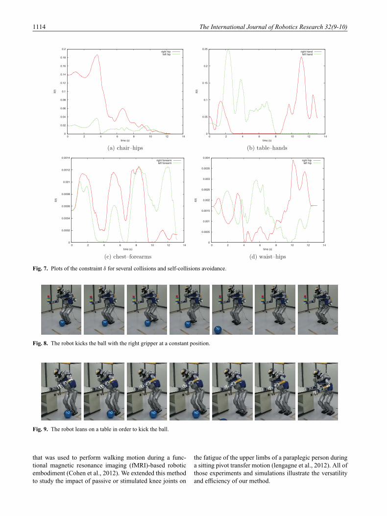
The chair-sitting scenario is chosen for its complexity andalso because we have a ground-truth on running it with dif-ferent control strategies (see, e.g., Escande et al., 2008).We however assess our multi-contact motion generator withseveral other experiments involving the HRP-2 humanoidrobot. In Lengagne et al. (2010a), we performed a kick-ing motion while making one hand stay still at a constantposition, see snapshots Figure 8. We also generate a kick-ing motion with the right arm gripper uses a table to supportthe motion. The contact between the gripper and the tableis put at the same position as the previous experiment inFigure 9. These experiments reveal also the difference in

posture and force distribution when the humanoid’s handuses an additional contact support for the kicking.

Using our method, we are certainly able to produce reg-ular walking motions. Since there are some non-modeledflexibilities we consider additional constraints to accountfor the dynamic effects during motion (Lengagne et al.,2011b). Hence, we are able to generate normal walking (cf.Figure 11) and also a walking motion stepping on a 15 cmplatform, see Figure 12 and (Lengagne et al., 2011b).

We are aware that more efficient state-of-the-art gaitedwalking pattern planners/controllers are able to generatethis kind of walking motions. We believe that our methodcan be used to design whole-body trajectories for COM-COP reduced-model-based walking pattern generators. But,more importantly, our method is able to consider (with-out any change in the software framework) some addi-tional constraints in order to reproduce leg impairments(Lengagne et al., 2011a) by setting a constant knee posi-tion to emulate a humanoid knee sprained and wearing asplint (Figure 13), or by setting maximal contact forces onone foot to emulate a broken or painful foot as illustratedby Figure 14.

We can also consider contact around the edge. We imple-mented a walking motion that reproduce the rotation aroundthe heels and toes as presented in Figure 15. Eventually, weperformed a throwing motion with the HRP-2 robot. Fig-ure 16 shows the execution of the motion for which thefoot steps were determined heuristically in order to mimica baseball player throwing.

Note that as all of these experiments are made open-loop(i.e. without attitude of force feedbacks), we use only thelocal joint position PD controller when at least one hand iscontacting the environment during the motion (Figures 9and 10). Otherwise, for the walking motions we use theHRP-2 embedded stabilizer presented in Kajita et al. (2005)in order to deal with the non-modeled flexibilities.

We also used our method to generate motions for theHOAP-3 humanoid robot and for a simulated model of thehuman. We built a motion database for the HOAP-3 robot


0

0.02

0.04

0.06

0.08

0.1

0.12

0.14

0.16

0.18

0.2

0 2 4 6 8 10 12 14

δ(t)

time (s)

right hipleft hip

(a) chair–hips

0

0.05

0.1

0.15

0.2

0.25

0 2 4 6 8 10 12 14

δ(t)

time (s)

right handleft hand

(b) table–hands

0

0.0002

0.0004

0.0006

0.0008

0.001

0.0012

0.0014

0 2 4 6 8 10 12 14

δ(t)

time (s)

right forearmleft forearm

(c) chest–forearms

0

0.0005

0.001

0.0015

0.002

0.0025

0.003

0.0035

0.004

0 2 4 6 8 10 12 14

δ(t)

time (s)

right hipleft hip

(d) waist–hips

Fig. 7. Plots of the constraint δ for several collisions and self-collisions avoidance.

Fig. 8. The robot kicks the ball with the right gripper at a constant position.

Fig. 9. The robot leans on a table in order to kick the ball.

that was used to perform walking motion during a func-tional magnetic resonance imaging (fMRI)-based roboticembodiment (Cohen et al., 2012). We extended this methodto study the impact of passive or stimulated knee joints on

the fatigue of the upper limbs of a paraplegic person duringa sitting pivot transfer motion (lengagne et al., 2012). All ofthose experiments and simulations illustrate the versatilityand efficiency of our method.


Fig. 10. With the right arm, the HRP-2 robot takes an additional support on the desk, which allows it to stably lean and put a ball intothe trash box located under the desk.

Fig. 11. Walking motion without additional constraints.

Fig. 12. The HRP-2 over crossing a 15 cm platform: the HRP-2 takes steps the platform with one foot and over-cross it with the other.

Fig. 13. Walking motion with a locked knee.

Fig. 14. Walking motion with a sore leg.

7. Discussions

We propose a versatile and effective method to generatedynamic and optimal multi-contact motions for humanoidrobots. We highlight through several typical complex sce-narios, its ability to generate complex motions that cannotbe computed using existing geometric planning methods ortask-function approaches.

Since we compute the entire motion over all of the phasesduring the same optimization process, we have an optimalmotion for the considered sequence of contact stances. Thegeneration of the sequence is based on quasi-static posturesin the multi-contact planner that provide us with the contactstances. We believe that it is possible to merge the compu-tation of the sequence of contact stances and the generationof the dynamic motion.


Fig. 15. The HRP-2 humanoid rotates around the edges during a walking motion.

Fig. 16. The robot throws a ball mimicking a baseball player.

Our method still requires a large amount of computa-tion time. To make it more attractive, we must decrease thecomputation time. There are several avenues to explore tofacilitate this. The first trivial one is to reduce the horizonof the preview window by feeding the solver with only theupcoming new two of three transitions rather than givingthe entire sequence of contacts. This option is interestingonly after reaching good computation performances sincethe method can then be transformed into a model-basednonlinear preview controller.

We currently use the L-BFGS approximation of the Hes-sian provided by the IPOPT solver (Wächter and Biegler,2006) that considers the Hessian matrix full. Indeed, regard-ing the decomposition of the motion into several phases andtime interval, it appears that Hessian matrix is sparse whichis not taken into account for the moment. An implementa-tion of a sparse L-BFGS method should help to decreasethe number of iterations, and hence the computation time.Another solution should be to include parallel architec-tures such as the general purpose graphics processing unit(GPGPU) in order to make use of parallel computation ofthe constraint and cost functions and of their gradients. Itis possible to parallelize at least the computation of eachtime interval [t]i that are independent from each other. Byconsidering these issues, it could be interesting to design anew solver that can use the computational efficiency of theGPGPU and exploit the sparse properties of the problemunder study.

Albeit the presence of the flexible parts and assuming aperfectly known environment, the motion is currently per-formed without any balance controller. Future work shouldfocus on the motion adaptation as presented by Lengagneet al. (2011c) and/or on a torque control law similar toSentis et al. (2010) that can deal with uncertainties regard-ing the position and orientation of the contact points, i.e.on the position and dimension of the table and chair in ourcase.

8. Conclusion

In this paper, we solve multi-contact transitions motionsusing nonlinear optimization techniques. Computed trajec-tories guarantee constraint satisfaction all over the timemotion whatever the time-grid size and accounts for allclassical robotic constraints including non-desired colli-sions avoidance. We experimented the computed trajec-tories on complex multi-contact scenarios involving theHRP-2 humanoid robot. As far as we know, there is no exist-ing method that can produce such complex multi-contactmotions. This is mainly due to the difficulties to model thedynamic balance and unilateral forces, to deal efficientlywith the continuous constraints and to integrate the collisionand self-collision in a safe way. We presented an analyti-cal formulation of the contact forces that is a counterpartto the dynamic effect and encompass the balance of therobot. To ensure the validity of the continuous constraintswe make use of Taylor series expansion approximations forthe models of the robot.

Our future work is now focused on building and improv-ing performance and robustness strategies in using effec-tively such a method in close interchange with low-levelcontrollers.

Notes

1. Note that the n-order basis functions used to evaluate extremaare different from the cubic basis function used to define thejoint trajectories in Equation (4.4).

2. We neglect the impacts at contact creation because we con-strain the landing speed at contact creations.

3. It is also very strongly suggested in all of the optimizationtextbooks (e.g. Gill et al., 1982, p. 5).

Funding

This work is partially supported by grants from the GermanResearch Foundation (DFG: Deutsche Forschungsgemeinschaft),


from the Japan Society for the Promotion of Science (JSPS;Grant-in-Aid for JSPS Fellows P09809 and for Scientific Research(B), 22300071, 2010), and from the RoboHow.Cog FP7 (seehttp://www.robohow.eu).

Acknowledgements

Authors would like to thank Dr Francois Keith and Pierre Ger-gondet for their help and assistance in making the simulation andexperiments.

References

Arisumi H, Miossec S, Chardonnet JR and Yokoi K (2008)Dynamic lifting by whole body motion of human robots. In:IEEE/RSJ International Conference on Intelligent Robots andSystems (IROS), pp. 668–675.

Benallegue M, Escande A, Miossec S and Kheddar A (2009)Fast C1 proximity queries using support mapping of sphere-torus-patches bounding volumes. In: IEEE InternationalConference on Robotics and Automation, 2009 (ICRA ’09),pp. 483–488.

Bendtsen C and Stauning O (1996) FADBAD, a Flexible C++Package for Automatic Differentation.

Berz M, Hoffstätter G and Atter GH (1998) Computation andapplication of Taylor polynomials with interval remainderbounds. Reliable Computing 4: 83–97.

Bobrow JE (1988) Optimal robot plant planning using theminimum-time criterion. IEEE Journal of Robotics andAutomation 4: 443–450.

Bouyarmane K, Escande A, Lamiraux F and Kheddar A (2009)Potential field guide for humanoid multicontacts acyclic motionplanning. In: IEEE International Conference on Robotics andAutomation.

Bouyarmane K and Kheddar A (2012) Humanoid robot loco-motion and manipulation step planning. Advanced Robotics(International Journal of the Robotics Society of Japan) 26:1099–1126.

Breteler MDK, Gielen SC and Meulenbroek RG (2001) End-pointconstraints in aiming movements: effects of approach angle andspeed. Biological Cybernetics 85(1): 65–75.

Cohen O, Druon S, Lengagne S, et al. (2012) fMRI basedrobotic embodiment: a pilot study. In: IEEE/RAS-EMBS Inter-national Conference on Biomedical Robotics and Biomecha-tronics (BioRob).

de Alwis T (2004) Maximizing or minimizing polynomials usingalgebraic inequalities. In: Proceedings of the 9th Asian Techno-logical Conference on Mathematics, Singapore, pp. 88–97.

de Boor C (1978) A Pratical Guide to Splines, volume 27. NewYork: Springer-Verlag.

Diehl M, Bock HG, Diedam H and Wieber PB (2006) Fast directmultiple shooting algorithms for optimal robot control. In:Diehl M and Mombaur K (eds.), Fast Motions in Biomechan-ics and Robotics (Lecture Notes in Control and InformationSciences, vol. 340). Berlin: Springer, pp. 65–93.

Escande A and Kheddar A (2009) Contact planning for acyclicmotion with tasks constraints. In: IEEE/RSJ International Con-ference on Intelligent Robots and Systems (IROS 2009).

Escande A, Kheddar A and Miossec S (2006) Planning supportcontact-points for humanoid robots and experiments on HRP-2. In: 2006 IEEE/RSJ International Conference on IntelligentRobots and Systems, Beijing, pp. 2974–2979.

Escande A, Kheddar A, Miossec S and Garsault S (2008) Planningsupport contact-points for acyclic motions and experiments onHRP-2. In: Khatib O, Kumar V and Pappas G (eds.), Interna-tional Symposium on Experimental Robotics, Athens, Greece(Springer Tracts in Advanced Robotics, number 54) Berlin:Springer-Verlag, pp. 293–302.

Escande A, Miossec S and Kheddar A (2007) Continuous gradi-ent proximity distance for humanoids free-collision optimized-postures. In: IEEE-RAS 7th International Conference onHumanoid Robots.

Gill PE, Murray W and Wright MH (1982) Practical optimization.New York: Academic Press.

Goswami A (1999) Postural stability of biped robots and the foot-rotation indicator (FRI) point. International Journal of RoboticResearch 18: 523–533.

Harada K, Kajita S, Kaneko K and Hirukawa H (2006) Dynamicsand balance of a humanoid robot during manipulation tasks.IEEE Transactions on Robotics 22: 568–575.

Hauser K, Bretl T and Latombe JC (2005) Non-gaited humanoidlocomotion planning. In: 2005 5th IEEE-RAS InternationalConference on Humanoid Robots, Tsukuba, pp. 7–12.

Hauser K and Latombe JC (2010) Multi-modal motion planningin non-expansive spaces. The International Journal of RoboticsResearch 29: 897–915.

Hettich R and Kortanek KO (1993) Semi-infinite programming:theory, methods, and applications. SIAM Review 35: 380–429.

Hirukawa H, Hattori S, Harada K, et al. (2006) A universal stabil-ity criterion of the foot contact of legged robots - adios ZMP. In:IEEE International Conference on Robotics and Automation(ICRA), pp. 1976–1983.

Hyon SH, Hale JG and Cheng G (2007) Full-body complianthuman–humanoid interaction: balancing in the presence ofunknown external forces. IEEE Transactions on Robotics 23:884–898.

Kajita S, Kanehiro F, Kaneko K, et al. (2003) Biped walkingpattern generation by using preview control of zero-momentpoint. In: IEEE International Conference on Robotics andAutomation, volume 2, pp. 1620–1626.

Kajita S, Nagasaki T, Kaneko K, Yokoi K and Tanie K (2005) Arunning controller of humanoid biped HRP-2LR. In: Proceed-ings of the 2005 IEEE International Conference on Roboticsand Automation, 2005 (ICRA 2005), pp. 616–622.

Kaneko K, Kanehiro F, Kajita S, et al. (2004) Humanoid robotHRP-2. In: Proceedings 2004 IEEE International Conferenceon Robotics and Automation, 2004 (ICRA ’04), vol. 2, pp.1083–1090.

Khalil W and Dombre E (2002) Modeling, Identification &Control of Robots, 3rd edn. Paris: Hermes Sciences Europe.

Lee SH and Goswami A (2012) A momentum-based balance con-troller for humanoid robots on non-level and non-stationaryground. Journal of Autonomous Robots 33: 399–414.

Lee SH, Kim J, Park F, Kim M and Bobrow JE (2005) Newton-type algorithms for dynamics-based robot movement optimiza-tion. IEEE Transactions on Robotics 21: 657–667.

Lee Y, Lengagne S, Kheddar A and Kim YJ (2012) Accurate eval-uation of a distance function for optimization-based motionplanning. In: IEEE/RSJ International Conference on IntelligentRobots and Systems IROS.

Lengagne S, Jovic J, Pierella C, Fraisse P and Coste CA(2012) Generation of multi-contact motions with passive joints:Improvement of sitting pivot transfer strategy for paraplegics.In: IEEE/RAS-EMBS International Conference on BiomedicalRobotics and Biomechatronics (BioRob).


Lengagne S, Kheddar A, Druon S and Yoshida E (2011a) Emu-lating human leg impairments and disabilities in walkingwith humanoid robots. In: IEEE International Conference onRobotics & Biomimetics.

Lengagne S, Kheddar A and Yoshida E (2011b) Considering float-ting contact and un-modeled effects for multi-contact motiongeneration. In: Workshop on Humanoid Service Robot Navi-gation in Crowded and Dynamic Environments at the IEEEHumanoids Conference.

Lengagne S, Mathieu P, Kheddar A and Yoshida E (2010a) Gen-eration of dynamic motions under continuous constraints: Effi-cient computation using B-splines and Taylor polynomials. In:IEEE/RSJ International Conference on Intelligent Robots andSystems (IROS).

Lengagne S, Mathieu P, Kheddar A and Yoshida E (2010b) Gen-eration of dynamic multi-contact motions: 2D case studies. In:IEEE-RAS Internationnal conference on Humanoid robots.

Lengagne S, Ramdani N and Fraisse P (2011c) Planning and fastreplanning safe motions for humanoid robots. IEEE Transac-tions on Robotics 27: 1095–1106.

Miossec S, Yokoi K and Kheddar A (2006) Development of a soft-ware for motion optimization of robots– application to the kickmotion of the HRP-2 robot. In: IEEE International Conferenceon Robotics and Biomimetics, pp. 299–304.

Mombaur KD, Bock HG, Schlöder JP and Longman RW (2005)Open-loop stable solutions of periodic optimal control prob-lems in robotics. Zeitschrift für Angewandte Mathematik undMechanik 85: 499–515.

Park FC, Bobrow JE and Ploen SR (1995) A lie group formula-tion of robot dynamics. The International Journal of RoboticsResearch 14: 609–618.

Piazzi A and Visioli A (1998) Global minimum-time trajectoryplanning of mechanical manipulators using interval analysis.International Journal of Control 71: 631–652.

Piazzi A and Visioli A (2000) Global minimum-jerk trajec-tory planning of robot manipulators. IEEE Transactions onIndustrial Electronics 47: 140–149.

Reemtsen R and Rückmann JJ (eds.) (1998) Nonconvex Optimiza-tion and Its Applications: Semi-infinite Programming. KluwerAcademic Publishers.

Righetti L, Buchli J, Mistry M and Schaal S (2011) Controlof legged robots with optimal distribution of contact forces.In: IEEE-RAS International Conference on Humanoid Robots,pp. 318–324.

Schultz G and Mombaur KD (2010) Modeling and optimalcontrol of human-like running. IEEE/ASME Transactions onMechatronics 15: 783–792.

Sentis L, Park J and Khatib O (2010) Compliant control of mul-ticontact and center-of-mass behaviors in humanoid robots.IEEE Transactions on Robotics 26: 483–501.

Steinbach MC (1997) Optimal Motion Design using InverseDynamics. Technical Report, Konrad-Zuse-Zentrum für Infor-mationstechnik Berlin.

Stephens BJ and Atkeson CG (2010) Dynamic balance force con-trol for compliant humanoid robots. In: IEEE/RSJ InternationalConference on Intelligent Robots and Systems, pp. 1248–1255.

Uno Y, Kawato M and Suzuki R (1989) Formation and con-trol of optimal trajectory in human multijoint arm movement.Biological Cybernetics 6(2): 89–101.

Von Stryk O (1993) Numerical solution of optimal control prob-lems by direct collocation. In Optimal Control (International

Series of Numerical Mathematics, vol. 111). Berlin: Springer,pp. 129–143.

Von Stryk O (1998) Optimal control of multibody systems in min-imal coordinates. Zeitschrift für Angewandte Mathematik undMechanik 78(S3): 1117–1120.

Vukobratovic M and Borovac B (2004) Zero-moment point:thirty five years of its life. International Journal of HumanoidRobotics 1: 157–173.

Wächter A and Biegler LT (2006) On the implementation ofa primal-dual interior point filter line search algorithm forlarge-scale nonlinear programming. Mathematical Program-ming 106: 22–57.

Zhang X, Redon S, Lee M and Kim YJ (2007) Continuous colli-sion detection for articulated models using taylor models andtemporal culling. ACM Transactions on Graphics 26(3): 15.

Appendix A: Analytical formulation of thecontact forces

A.1. Problem

Knowing the joint trajectories, we analytically compute thecontact forces in Equation (3.6), which can also be writtenas

F = −(JT2 ( q) )−1

D2 (.1)

Since the matrix J2 is not necessarily square, the pseudo-inverse: (JT

2 )+ =(J2JT2 )−1 J2 can be computed instead of

(JT2 )−1. By definition, the pseudo-inverse solves an equation

system that has more degrees of freedom than equations,which is our case, by minimizing the Euclidean norm of thesolution. Yet, our primary interest is not to minimize theEuclidean norm but to find a function f ( q, D2) that solvesthe contact forces which satisfy both Equation (3.6) and asmuch as possible Equation (3.4), that is

F = f ( q, D2) (.2)

We propose to find the analytic solution for the contactforces that reflects the balance of the robot, cf. Equation(3.6), and the friction constraints, Equation (3.4), i.e. theanalytic solution to the following problem:

min 12

∑i βi( αi||Ft

i ||2 + Fni

2)

∑i

([PiAi

Ai

][Fi]

)+ [D2] = 0

(.3)

In this formulation, we decompose JT2 through (i)Pi,

the screw operator of the contact position, and (ii) Ai

the orientation of the contact framework; [D2] =[Mx, My, Mz, Fx, Fy, Fz]T is the effort due to the free dynam-ics, βi a coefficient to equilibrate (or not) the repartition ofthe forces, αi is used to weight the tangential forces withregards to its corresponding normal force. The solution tothis problem ensures the dynamic equality constraint Equa-tion (3.6), but does not guarantee the feasibility of the con-tact forces that must be checked by the optimization solver.Note that defining ∀i βi = 1, αi = 1 is equivalent to solvethe pseudo-inverse problem.


A.2. Analytic solution

The resolution of this problem starts by writing theLagrangian:

L =∑

i

⎡⎣ βiαiF2

x,iβiαiF2

y,i

βiF2z,i

⎤⎦+

(∑i

[PiAi

Ai

][Fi] + [D2]

)[λ]

(.4)Here, we assume that the z-axis is the normal direc-

tion of the contact forces and define [λ] as the vector ofthe Lagrange multipliers. The optimal solution fulfills theoptimality condition:

∂L

∂( F◦,i, λj)= 0 (.5)

From the derivative with respect to Fi we have

Fi = −W−1i

[PiAi Ai

][λ] (.6)

with Wi = diag( βiαi, βiαi, βi). Then, we replace the contactforces expression in the set of the equality constraint and weget

� [λ] = − [D2] (.7)

with

� =∑

i

([PiAi

Ai

]W

−1i

[PiAi Ai

])(.8)

where � ∈ R6×6 is a 6 × 6 matrix that we can easily invert

using the Gauss–Jordan algorithm to find the value of theLagrange multipliers:

[λ] = −�−1 [D2] (.9)

Then, we put the Lagrange multipliers [λ] in Equation(.6) to get the value of the contact forces. Eventually, we areable to compute the contact forces from the joint trajectoriesand, using Equation (3.3), we can compute the joint torques.

Appendix B: Properties of the B-splines

We briefly present the properties of the B-splines that arerelevant during the motion generation process.

B.1. Control points

The first nicety is related to the computation of the deriva-tive of the state variables regarding the optimization param-eters. Since, at any time instant, the joint values rely onlyon four control points, we choose to define intervals so that,all along a time interval, the joint value relies only on fourcontrol points, see Figure 3. This avoids to compute thederivative regarding all the parameters since only a few ofthem have a non-null value.

B.2. Convex hull

B-splines (q( t)) is entirely contained in the convex hull ofits control points; that yields

if ∀i ∈ [1, m] q ≤ pi ≤ qthen ∀t ∈ [�t] q ≤ q( t) ≤ q

(.10)

We use this property to ensure the joint limits with-out implementing them as sets of continuous inequalityconstraints, but rather considering bounds directly on theoptimization parameters.

B.3. Derivative of a B-spline

The time derivative of a B-spline with m control points isanother B-splines parameterized with m − 1 control points.This is obtained by derivation of the Cox–de Boor recursion(de Boor, 1978) with respect to time t:

q( t) =m∑

i=1

bki ( t) pi =

m−1∑i=1

bk−1i ( t) ri (.11)

with

ri = k

ui+k+1 − ui+1( pi+1 − pi) (.12)

here k is the order of the B-spline basis functions, ui is theith component of the nodal vector as defined in (de Boor,1978). It is then possible to obtain a system of ( m − 1) lin-ear inequalities to impose joint speed limits, as we enforcedjoint position limits as bounds on the B-spline parameters.Thus, we add the following constraints:

q ≤ ri ≤ q (.13)

Extensions to upper derivatives follow in the same way.

B.4. Optimality

Hence, the obtained solution is very likely sub-optimal asthere is no reciprocal to Equation (.10). We already raisedthis issue in Lengagne et al. (2010a). Yet, the parameteriza-tion of the joint trajectories (by any method) leads already toa sub-optimal motion and we believe that there is a venuefor a thorough study on other possible parameterizations.Indeed, any kind of parameterization restricts the IP prob-lem’s solution for the chosen parameterization, which is defacto sub-optimal.

Appendix C: Index to Multimedia Extensions

The multimedia extension page is found at http://www.ijrr.org

Table of Multimedia Extensions

Extension Type Description

1 Video Experimental Validations

Documents

dynamic multi-contact motions © The Author(s) 2013 multi-contact motions The International Journal of ... satisfaction guaranteed motions for any time grid. ... and dynamic multi-contact