Dynamic Modeling and Power Modeling of Robotic Skid ...cdn.intechopen.com/pdfs/22305.pdf · Section 1 is the introduction. Section 2 presents ... model of a skid-steered vehicle was

Wei Yu, Emmanuel Collins and Oscar ChuyFlorida State University

U.S.A

1. Introduction

Dynamic models and power models of autonomous ground vehicles are needed to enablerealistic motion planning Howard & Kelly (2007); Yu et al. (2010) in unstructured, outdoorenvironments that have substantial changes in elevation, consist of a variety of terrainsurfaces, and/or require frequent accelerations and decelerations.At least 4 different motion planning tasks can be accomplished using appropriate dynamicand power models:

1. Time optimal motion planning.

2. Energy efficient motion planning.

3. Reduction in the frequency of replanning.

4. Planning in the presence of a fault, such as flat tire or faulty motor.

For the purpose of motion planning this chapter focuses on developing dynamic and powermodels of a skid-steered wheeled vehicle to help the above motion planning tasks. Thedynamic models are the foundation to derive the power models of skid-steered wheeledvehicles. The target research platform is a skid-steered vehicle. A skid-steered vehicle canbe either tracked or wheeled . Fig. 1 shows examples of a skid-steered wheeled vehicle and askid-steered tracked vehicle.This chapter is organized into five sections. Section 1 is the introduction. Section 2 presentsthe kinematic models of a skid-steered wheeled vehicle, which is the preliminary knowledgeto the proposed dynamic model and power model. Section 3 develops analytical dynamicmodels of a skid-steered wheeled vehicle for general 2D motion. The developed modelsare characterized by the coefficient of rolling resistance, the coefficient of friction, and theshear deformation modulus, which have terrain-dependent values. Section 4 developsanalytical power models of a skid-steered vehicle and its inner and outer motors in general2D curvilinear motion. The developed power model builds upon a previously developeddynamic model in Section 3. Section 5 experimentally verifies the proposed dynamic modelsand power models of a robotic skid-steered wheeled vehicle.Ackerman steering, differential steering, and skid steering are the most widely used steeringmechanisms for wheeled and tracked vehicles. Ackerman steering has the advantages of goodlateral stability when turning at high speeds, good controllability Siegwart & Nourbakhsh(2005) and lower power consumption Shamah et al. (2001), but has the disadvantages oflow maneuverability and need of an explicit mechanical steering subsystem Mandow et al.

Dynamic Modeling and Power Modeling of Robotic Skid-Steered Wheeled Vehicles

14

www.intechopen.com

2 Will-be-set-by-IN-TECH

Fig. 1. Examples of skid-steered vehicles: (Left) Skid-steered wheeled vehicle, (Right)Skid-steered tracked vehicle

(2007); Shamah et al. (2001); Siegwart & Nourbakhsh (2005). Differential steering is popularbecause it provides high maneuverability with a zero turning radius and has a simple steeringconfiguration Siegwart & Nourbakhsh (2005); Zhang et al. (1998). However, it does nothave strong traction and mobility over rough and loose terrain, and hence is seldom usedfor outdoor terrains. Like differential steering, skid steering leads to high maneuverabilityCaracciolo et al. (1999); Economou et al. (2002); Siegwart & Nourbakhsh (2005), faster responseMartinez et al. (2005), and also has a simple Mandow et al. (2007); Petrov et al. (2000); Shamahet al. (2001) and robust mechanical structure Kozlowski & Pazderski (2004); Mandow et al.(2007); Yi, Zhang, Song & Jayasuriya (2007). In contrast, it also leads to strong traction andhigh mobilityPetrov et al. (2000), which makes it suitable for all-terrain traversal.Many of the difficulties associated with modeling and operating both classes of skid-steeredvehicles arise from the complex wheel (or track) and terrain interaction Mandow et al. (2007);Yi, Song, Zhang & Goodwin (2007). For Ackerman-steered or differential-steered vehicles,the wheel motions may often be accurately modeled by pure rolling, while for skid-steeredvehicles in general curvilinear motion, the wheels (or tracks) roll and slide at the same timeMandow et al. (2007); O. Chuy et al. (2009); Yi, Song, Zhang & Goodwin (2007); Yi, Zhang,Song & Jayasuriya (2007). This makes it difficult to develop kinematic and dynamic modelsthat accurately describe the motion. Other disadvantages are that the motion tends to beenergy inefficient, difficult to control Kozlowski & Pazderski (2004); Martinez et al. (2005),and for wheeled vehicles, the tires tend to wear out faster Golconda (2005).A kinematic model of a skid-steered wheeled vehicle maps the wheel velocities to the vehiclevelocities and is an important component in the development of a dynamic model. Incontrast to the kinematic models for Ackerman-steered and differential-steered vehicles, thekinematic model of a skid-steered vehicle is dependent on more than the physical dimensionsof the vehicle since it must take into account vehicle sliding and is hence terrain-dependentMandow et al. (2007); Wong (2001). In Mandow et al. (2007); Martinez et al. (2005) a kinematicmodel of a skid-steered vehicle was developed by assuming a certain equivalence with akinematic model of a differential-steered vehicle. This was accomplished by experimentallydetermining the instantaneous centers of rotation (ICRs) of the sliding velocities of the left

292 Mobile Robots – Current Trends

www.intechopen.com

Dynamic Modeling and Power Modeling of Robotic Skid-steered Wheeled Vehicles 3

and right wheels. An alternative kinematic model that is based on the slip ratios of the wheelshas been presented in Song et al. (2006); Wong (2001). This model takes into account thelongitudinal slip ratios of the left and right wheels. The difficulty in using this model is theactual detection of slip, which cannot be computed analytically. Hence, developing practicalmethods to experimentally determine the slip ratios is an active research area Endo et al.(2007); Moosavian & Kalantari (2008); Nagatani et al. (2007); Song et al. (2008).To date, there is very little published research on the experimentally verified dynamic modelsfor general motion of skid-steered vehicles, especially wheeled vehicles. The main reason isthat it is hard to model the tire (or track) and terrain interaction when slipping and skiddingoccur. (For each vehicle wheel, if the wheel linear velocity computed using the angularvelocity of the wheel is larger than the actual linear velocity of the wheel, slipping occurs,while if the computed wheel velocity is smaller than the actual linear velocity, skiddingoccurs.) The research of Caracciolo et al. (1999) developed a dynamic model for planar motionby considering longitudinal rolling resistance, lateral friction, moment of resistance for thevehicle, and also the nonholonomic constraint for lateral skidding. In addition, a model-basednonlinear controller was designed for trajectory tracking. However, this model uses Coulombfriction to describe the lateral sliding friction and moment of resistance, which contradicts theexperimental results Wong (2001); Wong & Chiang (2001). In addition, it does not considerany of the motor properties. Furthermore, the results of Caracciolo et al. (1999) are limited tosimulation without experimental verification.The research of Kozlowski & Pazderski (2004) developed a planar dynamic model of askid-steered vehicle, which is essentially that of Caracciolo et al. (1999), using a differentvelocity vector (consisting of the longitudinal and angular velocities of the vehicle insteadof the longitudinal and lateral velocities). In addition, the dynamics of the motors, though notthe power limitations, were added to the model. Kinematic, dynamic and motor level controllaws were explored for trajectory tracking. However, as in Caracciolo et al. (1999), Coulombfriction was used to describe the lateral friction and moment of resistance, and the results arelimited to simulation. In Yi, Song, Zhang & Goodwin (2007) a functional relationship betweenthe coefficient of friction and longitudinal slip is used to capture the interaction between thewheels and ground, and further to develop a dynamic model of skid-steered wheeled vehicle.Also, an adaptive controller is designed to enable the robot to follow a desired trajectory. Theinputs of the dynamic model are the longitudinal slip ratios of the four wheels. However,the longitudinal slip ratios are difficult to measure in practice and depend on the terrainsurface, instantaneous radius of curvature, and vehicle velocity. In addition, no experiment isconducted to verify the reliability of the torque prediction from the dynamic model and motorsaturation and power limitations are not considered. In Wang et al. (2009) the dynamic modelfrom Yi, Song, Zhang & Goodwin (2007) is used to explore the motion stability of the vehicle,which is controlled to move with constant linear velocity and angular velocity for each half ofa lemniscate to estimate wheel slip. As in Yi, Song, Zhang & Goodwin (2007), no experimentis carried out to verify the fidelity of the dynamic model.The most thorough dynamic analysis of a skid-steered vehicle is found in Wong (2001); Wong& Chiang (2001), which consider steady-state (i.e., constant linear and angular velocities)dynamic models for circular motion of tracked vehicles. A primary contribution of thisresearch is that it proposes and then provides experimental evidence that in the track-terraininteraction the shear stress is a particular function of the shear displacement. This modeldiffers from the Coulomb model of friction, adopted in Caracciolo et al. (1999); Kozlowski& Pazderski (2004), which essentially assumes that the maximum shear stress is obtained as

293Dynamic Modeling and Power Modeling of Robotic Skid-Steered Wheeled Vehicles

www.intechopen.com


soon as there is any relative movement between the track and the ground. This research alsoprovides detailed analysis of the longitudinal and lateral forces that act on a tracked vehicle.But their results had not been extended to skid-steered wheeled vehicles. In addition, they donot consider vehicle acceleration, terrain elevation, actuator limitations, or the vehicle controlsystem.In the existing literature there are very few publications that consider power modeling ofskid-steered vehicles. The research of Kim & Kim (2007) provides an energy model of askid-steered wheeled vehicle in linear motion. This model is essentially the time integration ofa power model and is derived from the dynamic model of a motor, including the energy lossdue to the armature resistance and viscous friction as well as the kinetic energy of the vehicle.This research also uses the energy model to find the velocity trajecotry that minimizes theenergy consumption. However, the energy model only considers the dynamics of the motor,but does not include the mechanical dynamics of the vehicle and hence ignores the substantialenergy consumption due to sliding friction. Because longitudinal friction and moment ofresistance lead to substantial power loss when a skid steered vehicle is in general curvilinearmotion, the results of Kim & Kim (2007) cannot be readily extended to motion that is notlinear.The most thorough exploration of power modeling of a skid-steered (tracked) vehicle ispresented in Morales et al. (2009) and Morales et al. (2006). This research develops anexperimental power model of a skid-steered tracked vehicle from terrain’s perspective. Thepower model includes the power loss drawn by the terrain due to sliding frictions, and also thepower losses due to the traction resistance and the motor drivers. Based on another conceptualmodel, this research considers the case in which the inner track has the same velocity sign asthe outer track and qualitatively describes the negative sliding friction of the inner track, whichleads the corresponding motor to work as a generator. Experiments to apply the power modelfor navigation are also described. However, this research has two limitations that the currentresearch seeks to overcome. First, as in Caracciolo et al. (1999); Kozlowski & Pazderski (2004),discussed above in the context of dynamic modeling of skid-steered vehicles, Coulomb’s lawis adopted to describe the sliding friction component in the power modeling, which can leadto incorrect predictions for larger turning radii. Second, since the power model is derivedfrom the perspective of the terrain drawing power from the tracks, it does not appear possibleto quantify the power consumption of the left and right side motors. This is important sincethe motion of the vehicles can be dependent upon the power limitations of the motors.Building upon the research in Wong (2001); Wong & Chiang (2001), this chapter will developdynamic models of a skid-steered wheeled vehicle for general curvilinear planar (2D) motion.As in Wong (2001); Wong & Chiang (2001) the modeling is based upon the functionalrelationship of shear stress to shear displacement. Practically, this means that for a vehicletire the shear stress varies with the turning radius. This chapter also includes models of thesaturation and power limitations of the actuators as part of the overall vehicle model.Using the developed dynamic model for 2D general curvilinear motion, this chapter will alsodevelop power models of a skid-steered wheeled vehicle based on separate power modelsfor left and right motors. The power model consists of two parts: (1) the mechanical powerconsumption, including the mechanical loss due to sliding friction and moment of resistance,and the power used to accelerate vehicle; and (2) the electrical power consumption, which isthe electrical loss due to the motor electrical resistance. The mechanical power consumptionis derived completely from the dynamic model, while the electrical power consumption isderived using the electric current predicted from this dynamic model along with circuit


www.intechopen.com


theory. This chapter also discusses the interesting phenomenon that while the outer motoralways consumes power, even though the velocity of inner wheel is always positive, as theturning radius decreases from infinity (corresponding to linear motion), the inner motor firstconsumes power, then generates power, and finally consumes power again.In summary, we expect this chapter to make the following two fundamental contributions todynamic modeling and power modeling of skid-steered wheeled vehicles:

1. A paradigm for deriving dynamic models of skid-steered wheeled vehicles. Themodeling methodology will result in terrain-dependent models that describe generalgeneral planar (2D) motion.

2. A paradigm for deriving power models of skid-steered wheeled vehicles based ondynamic models. The power model of a skid-steered vehicle will be derived from vehicledynamic models. The power model will be described from the perspective of the motorsand includes both the mechanical power consumption and electrical power consumption.It can predict when a given trajectory is unachievable because the power limitation of oneof the motors is violated.

2. Kinematics of a skid-steered wheeled vehicle

In this section, the kinematic model of a skid-steered wheeled vehicle is described anddiscussed. It is an important component in the development of the overall dynamic modelsand power models of a skid-steered wheeled vehicle.To mathematically describe the kinematic models that have been developed for skid-steeredvehicles, consider a wheeled vehicle moving at constant velocity about an instantaneouscenter of rotation as shown in Fig. 2.The global and local coordinate frames are denoted respectively by X-Y and x-y. The variablesv, ϕ and R are respectively the translational velocity, angular velocity and turning radius ofvehicle. The instantaneous centers of rotation for the left wheel and right wheel are givenrespectively by ICRl and ICRr. Note that ICRl and ICRr are the centers for left and rightwheel treads (the parts of the tires that contact and slide on the terrain) Wong & Chiang(2001); Yi, Zhang, Song & Jayasuriya (2007), i.e., they are the centers for the sliding velocitiesof these contacting treads, but not the centers for the actual velocities of each wheel. It hasbeen shown that the three ICRs are in the same line, which is parallel to the x-axis of the localframe Mandow et al. (2007); Yi, Zhang, Song & Jayasuriya (2007).In the x-y frame, the coordinates of ICR, ICRl and ICRr are described as (xICR, yICR),(xICRl , yICRl) and (xICRr, yICRr). The vehicle velocity is denoted as u = [vx vy ϕ]T , wherevx and vy are the components of v along the x and y axes. The angular velocities of the left andright wheels are denoted respectively by ωl and ωr. (Note that for both the left and right sideof the vehicle the velocities of the front and rear wheels are the same since they are driven bythe same belt, and hence, there is only one velocity associated with each side.) The parametersb, B and r are respectively the wheel width, the vehicle width, and the wheel radius.An experimental kinematic model of a skid-steered wheeled vehicle that is developed inMandow et al. (2007) is given by

⎡

⎣

vx

vy

ϕ

⎤

⎦ =r

xICRr − xICRl

⎡

⎣

−yICR yICR

xICRr −xICRl

−1 1

⎤

⎦

[

ωl

ωr

]

(1)


www.intechopen.com


Fig. 2. The kinematics of a skid-steered wheeled vehicle and the correspondinginstantaneous centers of rotation (ICRs)

If the skid-steered wheeled vehicle is symmetric about the x and y axes, then yICRl = yICRr =0 and xICRl = −xICRr. Define the expansion factor α as the ratio of the longitudinal distancebetween the left and right wheels over the vehicle width, i.e.,

α �xICRr − xICRl

B. (2)

Then, for a symmetric vehicle the kinematic model (1) can be expressed as

[

vy

ϕ

]

=r

αB

[

αB2

αB2

−1 1

] [

ωl

ωr

]

. (3)

(Note that vx = 0.)The expansion factor α varies with the terrain. Experimental results show that the largerthe rolling resistance, the larger the expansion factor. For a Pioneer 3-AT, α = 1.5 for avinyl lab surface and α > 2 for a concrete surface. Equation (3) shows that the kinematicmodel of a skid-steered wheeled vehicle of width B is equivalent to the kinematic model ofa differential-steered wheeled vehicle of width αB. Note that when α = 1, (3) becomes thekinematic model for a differential-steered wheeled vehicle.A more rigorously derived kinematic model for a skid-steered vehicle is presented inMoosavian & Kalantari (2008); Song et al. (2006); Wong (2001). This model takes into accountthe longitudinal slip ratios il and ir of the left and right wheels and for symmetric vehicles isgiven by

[

vy

ϕ

]

=r

B

[

(1−il)B2

(1−ir)B2

−(1 − il) (1 − ir)

]

[

ωl

ωr

]

, (4)


www.intechopen.com


where il � (rωl − vl_a)/(rωl), ir � (rωr − vr_a)/(rωr) and vl_a and vr_a are the actualvelocities of the left and right wheels. We have found that when

ilir

= −ωr

ωland α =

1

1 − 2il iril+ir

, (5)

(3) and (4) are identical. Currently, to our knowledge no analysis or experiments havebeen performed to verify the left hand equation in (5) and analyze its physical significance.However, for a limited range of turning radii experimentally derived expressions for il/ir,essentially in terms of ωl and ωr, are given in Endo et al. (2007); Nagatani et al. (2007).

3. Dynamic modeling of a skid-steered wheeled vehicle

This section develops dynamic models of a skid-steered wheeled vehicle for the cases ofgeneral 2D motion. In contrast to dynamic models described in terms of the velocity vectorof the vehicle Caracciolo et al. (1999); Kozlowski & Pazderski (2004), the dynamic modelshere are described in terms of the angular velocity vector of the wheels. This is because thewheel (specifically, the motor) velocities are actually commanded by the control system, sothis model form is particularly beneficial for control and planning.Following Kozlowski & Pazderski (2004), the dynamic model considering the nonholonomicconstraint is given by

Mq + C(q, q) + G(q) = τ, (6)

where q = [θl θr]T is the angular displacement of the left and right wheels, q = [ωl ωr]T isthe angular velocity of the left and right wheels, τ = [τl τr]T is the torque of the left and rightmotors, M is the mass matrix, C(q, q) is the resistance term, and G(q) is the gravitational term.The primary focus of the following subsection is the derivation of C(q, q) to properly modelthe ground and wheel interaction. In the following content, it is assumed that the vehicle issymmetric and the center of gravity (CG) is at the geometric center.When the vehicle is moving on a 2D surface, it follows from the model given in Kozlowski &Pazderski (2004), which is expressed in the local x-y coordinates, and the kinematic model (3)that M in (6) is given by

M =

[

mr2

4 + r2 IαB2

mr2

4 − r2 IαB2

mr2

4 − r2 IαB2

mr2

4 + r2 IαB2

]

, (7)

where m and I are respectively the mass and moment of inertia of the vehicle. Since we areconsidering planar motion, G(q) = 0. C(q, q) represents the resistance resulting from theinteraction of the wheels and terrain, including the rolling resistance, sliding frictions, andthe moment of resistance, the latter two of which are modeled using Coulomb friction inCaracciolo et al. (1999); Kozlowski & Pazderski (2004). Assume that q = [ωl ωr]T is a knownconstant, then q = 0 and (6) becomes

C(q, q) = τ. (8)

Previous research Caracciolo et al. (1999); Kozlowski & Pazderski (2004) assumed that theshear stress takes on its maximum magnitude as soon as a small relative movement occursbetween the contact surface of the wheel and terrain. Instead of using this theory for trackedvehicle, Wong (2001) and Wong & Chiang (2001) present experimental evidence to show thatthe shear stress of the tread is function of the shear displacement. The maximum shear stressis practically achieved only when the shear displacement exceeds a particular threshold. Inthis section, this theory will be applied to a skid-steered wheeled vehicle.


www.intechopen.com


Based on the theory in Wong (2001); Wong & Chiang (2001), the shear stress τss and sheardisplacement j relationship can be described as,

τss = pμ(1 − e−j/K), (9)

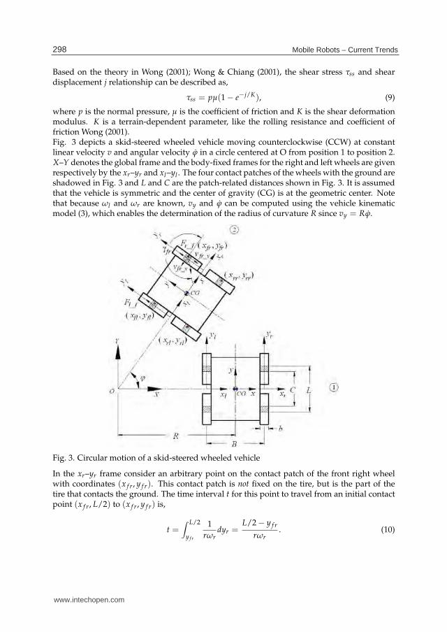
where p is the normal pressure, μ is the coefficient of friction and K is the shear deformationmodulus. K is a terrain-dependent parameter, like the rolling resistance and coefficient offriction Wong (2001).Fig. 3 depicts a skid-steered wheeled vehicle moving counterclockwise (CCW) at constantlinear velocity v and angular velocity ϕ in a circle centered at O from position 1 to position 2.X–Y denotes the global frame and the body-fixed frames for the right and left wheels are givenrespectively by the xr–yr and xl–yl . The four contact patches of the wheels with the ground areshadowed in Fig. 3 and L and C are the patch-related distances shown in Fig. 3. It is assumedthat the vehicle is symmetric and the center of gravity (CG) is at the geometric center. Notethat because ωl and ωr are known, vy and ϕ can be computed using the vehicle kinematicmodel (3), which enables the determination of the radius of curvature R since vy = Rϕ.

Fig. 3. Circular motion of a skid-steered wheeled vehicle

In the xr–yr frame consider an arbitrary point on the contact patch of the front right wheelwith coordinates (x f r, y f r). This contact patch is not fixed on the tire, but is the part of thetire that contacts the ground. The time interval t for this point to travel from an initial contactpoint (x f r, L/2) to (x f r, y f r) is,

t =∫ L/2

y f r

1

rωrdyr =

L/2 − y f r

rωr. (10)


www.intechopen.com


During the same time, the vehicle has moved from position 1 to position 2 with an angulardisplacement of ϕ. The sliding velocities of point (x f r, y f r) in the xr and yr directions aredenoted by v f r_x and v f r_y. Therefore,

v f r_x = −y f r ϕ, v f r_y = (R + B/2 + x f r)ϕ − rωr. (11)

The resultant sliding velocity v f r and its angle γ f r in the xr-yr frame are

v f r =√

v2f r_x + v2

f r_y, γ f r = π + arctan

(

v f r_y

v f r_x

)

. (12)

Note that when the wheel is sliding, the direction of friction is opposite to the sliding velocity,and if the vehicle is in pure rolling, v f r_x and v f r_y are zero.In order to calculate the shear displacement of this reference point, the sliding velocities needto be expressed in the global X–Y frame. Let v f r_X and v f r_Y denote the sliding velocities in theX and Y directions. Then, the transformation between the local and global sliding velocitiesis given by,

[

v f r_X

v f r_Y

]

=

[

cos ϕ − sin ϕsin ϕ cos ϕ

] [

v f r_x

v f r_y

]

. (13)

The shear displacements j f r_X and j f r_Y in the X and Y directions can be expressed as

j f r_X =∫ t

0v f r_Xdt =

∫ L/2

y f r

(v f r_x cos ϕ − v f r_y sin ϕ)1

rωrdyr

= (R + B/2 + x f r) · {cos

[

(L/2 − y f r)ϕ

rωr

]

− 1} − y f r sin

[

(L/2 − y f r)ϕ

rωr

]

, (14)

j f r_Y =∫ t

0v f r_Ydt =

∫ L/2

y f r

(v f r_x sin ϕ + v f r_y cos ϕ)1

rωrdyr

= (R + B/2 + x f r) · sin

[

(L/2 − y f r)ϕ

rωr

]

− L/2 + y f r cos

[

(L/2 − y f r)ϕ

rωr

]

. (15)

The resultant shear displacement j f r in the X–Y frame is given by, j f r =√

j2f r_X + j2f r_Y .

Similarly, it can be shown that for the reference point (xrr, yrr) in the rear right wheel theangle of the sliding velocity γrr in the xr-yr frame is

γrr = arctan

[

(R + B/2 + xrr)ϕ − rωr

−yrr ϕ

]

, (16)

and the shear displacements jrr_X and jrr_Y are given by

jrr_X = (R + B/2 + xrr) · {cos

[

(−C/2 − yrr)ϕ

rωr

]

− 1} − yrr sin

[

(−C/2 − yrr)ϕ

rωr

]

, (17)

jrr_Y = (R + B/2 + xrr) · sin

[

(−C/2 − yrr)ϕ

rωr

]

+ C/2 + yrr cos

[

(−C/2 − yrr)ϕ

rωr

]

. (18)


www.intechopen.com


and the magnitude of the resultant shear displacement jrr is jrr =√

j2rr_X + j2rr_Y .

The friction force points in the opposite direction of the sliding velocity. Using j f r and jrr,derived above, with (9) and integrating along the contact patches yields that the longitudinalsliding friction of the right wheels Fr_ f can be expressed as

Fr_ f =∫ L/2

C/2

∫ b/2

−b/2prμr(1 − e−j f r/Kr ) sin(π + γ f r)dxrdyr

+∫ −C/2

−L/2

∫ b/2

−b/2prμr(1 − e−jrr/Kr ) sin(π + γrr)dxrdyr, (19)

where pr, μr and Kr are respectively the normal pressure, coefficient of friction, and sheardeformation modulus of the right wheels. While most of the parameters in (19) can be directlymeasured, as discussed further below, the parameters μr and Kr must be estimated.Let fr_r denote the rolling resistance of the right wheels, including the internal locomotionresistance such as resistance from belts, motor windings and gearboxes Morales et al. (2006).The complete resistance torque τr_Res from the ground to the right wheel is given by

τr_Res = r(Fr_ f + fr_r). (20)

Since ωr is constant, the input torque τr from right motor will compensate for the resistancetorque, such that

τr = τr_Res. (21)

The above discussion is for the right wheels. Exploiting the same derivation process, one canobtain analytical expressions for the shear displacements j f l and jrl of the front and rear leftwheels, and the angles of the sliding velocity γ f l and γrl . The longitudinal sliding friction ofthe left wheels Fl_ f is then given by

Fl_ f =∫ L/2

C/2

∫ b/2

−b/2plμl(1 − e−j f l /Kl ) sin(π + γ f l)dxldyl

+∫ −C/2

−L/2

∫ b/2

−b/2plμl(1 − e−jrl /Kl ) sin(π + γrl)dxldyl , (22)

where pl , μl and Kl are respectively the normal pressure, coefficient of friction, and sheardeformation modulus of the left wheels. Denote the rolling resistance of the left wheels asfl_r. The input torque τl of the left motor equals the resistance torque of the left wheel τl_Res,such that

τl = τl_Res = r(Fl_ f + fl_r). (23)

Fig. 4 compares the resistance torque prediction of τl_Res and τr_Res using shear stress andshear displacement function (9) and Coulomb’s law when the skid-steered wheeled vehicle ofFig. 13 is in steady state rotation.

τss = pμ (Coulomb′s Law) (24)

It is seen that Coulomb’s law leads to a resistance torque that has the same constant value forall turning radii, which contradicts the experimental results shown in Wong (2001); Wong &Chiang (2001) for tracked vehicles and below in Fig. 15 for wheeled vehicles.Using (21) and the left equation of (23) with (8) yields

C(q, q) = [τl_Res τr_Res]T . (25)


www.intechopen.com


Fig. 4. Inner and outer motor resistance torque prediction using function (9) and Coulomb’slaw when vehicle is in steady state rotation.

Substituting (7), (25) and G(q) = 0 into (6) yields a dynamic model that can be used to predict2D movement for the skid-steered vehicle:

⎡

⎣

mr2

4 + r2 IαB2

mr2

4 − r2 IαB2

mr2

4 − r2 IαB2

mr2

4 + r2 IαB2

⎤

⎦ q +

[

τl_Res

τr_Res

]

=

[

τl

τr

]

. (26)

In summary, in order to obtain (25), the shear displacement calculation of (14), (15), (17)and (18) is the first step. The inputs to these equations are the left and right wheel angularvelocities ωl and ωr. The shear displacements are employed in (19) and (22) to obtain theright and left sliding friction forces, Fr_ f and Fl_ f . Next, the sliding friction forces and rollingresistances are substituted into (20) and (23) to calculate the right and left resistance torques,which determine C(q, q) using (25).

4. Power modeling of a skid-steered wheeled vehicle

This section derives power models for a skid-steered wheeled vehicle, moving as in Fig.3. The foundation for modeling the power consumption model is the dynamic model ofSection 3. The power consumption for each side of the vehicle includes the mechanical powerconsumption due to the motion of the wheels and the electrical power consumption due tothe electrical resistance of the motors. The total power consumption of the vehicle is the sumof the power consumption of of the left and right sides.Assume that a skid-steered wheeled vehicle moves CCW about an instantaneous center ofrotation (see Fig. 3). The circuit diagram for each side of the vehicle is shown in Fig. 5. Eachcircuit includes a battery, motor controller, motor M and the motor electrical resistance Re.In Fig. 5 ωl and ωr are the angular velocities of the left and right wheels, Ul and Ur are theoutput voltages of the left and right motor controllers, and il and ir are the currents of the left


www.intechopen.com


Fig. 5. The circuit layout for the left and right side of a skid-steered wheeled vehicle.

and right circuits. For the experimental vehicle used in this research (the modified Pioneer3-AT shown in Fig. 13), ωl and ωr are always positive1.The electric model of a DC motor at steady state is given by Rizzoni (2000),

Va = Eb + Ra Ia, (27)

where Va is the supply voltage to the motor, Ra is the motor armature resistance, Ia is themotor current, and Eb is the back EMF. The power consumption Pa of a DC motor is given byPa = Va Ia. Hence, multiplying (27) by Ia yields

Pa = Va Ia = Pe + Ra I2a , (28)

where Pe is the portion of the electric power converted to mechanical power by the motor andis given by

Pe = Eb Ia. (29)

The mechanical power Pm of a DC motor is given by

Pm = ωmτ, (30)

where ωm and τ are respectively the angular velocity and applied torque of the motor. Forideal energy-conversion case Rizzoni (2000),

Pm = Pe. (31)

Substituting (29), (30) and (31) into (28) yields the power model of a DC motor used in theanalysis of this research,

Pa = ωmτ + Ra I2a . (32)

In (32), the first term is the mechanical power consumption, which includes the power tocompensate the left and right sliding frictions and the moment of resistance along with thepower to accelerate the motor, and the second term is the electrical power consumption dueto the motor electric resistance, which is dissipated as heat.Using (32), the power consumed by the right motor Pr can be expressed as,

Pr = Urir = Pr,m + Pr,e, (33)

1 Due to the torque limitations of the motors in the experimental vehicle, the minimum achievableturning radius is larger than half the width of the vehicle. This implies that the instantaneous radius ofcurvature is located outside of the vehicle body so that ωl and ωr are always positive.


www.intechopen.com


where Pr,m and Pr,e are the mechanical power consumption and the electrical powerconsumption for the right side motor. In non ideal case, Pr,m and Pr,e in (33) are,

Pr,m =τrωr

η, (34)

Pr,e = i2r Re, (35)

where τr and ωr are the same as in (26) in Section 3, and η is the motor efficiency.For the right side motor, the output torque τr determined from the dynamic model (26) isgiven by

τr = KT irgrη, (36)

where KT is the torque constant and gr is the gear ratio. So the required current in right sideof motor is,

ir =τr

KT grη. (37)

Plugging (37) into (35) yields,

Pr,e = (τr

KT grη)2Re. (38)

Substituting (34) and (38) into (33), the power model for the right (outer) motor is,

Pr =τrωr

η+ (

τr

KT grη)2Re. (39)

Notice that the only variables in (39) is the applied torques τr along with the angular velocitiesωr, which are available from the dynamic model in Chapter 3.Similarly, for the left (inner) part of vehicle,

Pl = Ul il = Pl,m + Pl,e, (40)

Pl,m =τlωl

η, (41)

Pl,e = i2l Re, (42)

τl = KT il , (43)

Pl,e = (τl

KT grη)2Re, (44)

Pl =τlωl

η+ (

τl

KT grη)2Re. (45)

Let P denote the power that must be supplied by the motor drivers to the motors to enable themotion of a of a skid-steered wheeled vehicle and define the operator σ : R → R such that

σ(Q) =

{

Q : Q ≥ 00 : Q < 0.

(46)

Then the entire power model of a skid-steered wheeled vehicle is,

P = σ(Pr) + σ(Pl). (47)

Typically, one might expect to write P = Pr + Pl . However, since it turns out that Pl can benegative and that this generated power does not charge the battery in our research vehicle,


www.intechopen.com


the more general form (47) is used. To enable the battery to be charged requires modificationsof the motor controller, which was beyond the scope of this project.In summary, given the input of the left wheel and right wheel angular velocities ωl and ωr, thefirst step in computing (45) and (39), the power models of the left motors and right motors,is the calculation of the left wheel and right wheel sliding frictions Fl_ f and Fr_ f using (22)and (19). The sliding frictions along with experimentally determined values of the rollingresistances fl_r and fr_r are then substituted into (23) and (20) to obtain the resistance torquesτl_Res and τr_Res, which are in turn substituted into the vehicle dynamic model (26) to obtainthe left wheel and right wheel torques τl and τr. Next, the left and right wheel torques aresubstituted into (45) and (39) to calculate the power consumption of the left and right wheels.The entire power consumption of the vehicle may then computed by substituting (45) and (39)into (47). While (45) and (39) are general equations for all DC motor driven vehicles, the τl

and τr in (45) and (39) have to be calculated specifically from the skid-steered dynamic model(26).

4.1 Power models analysis

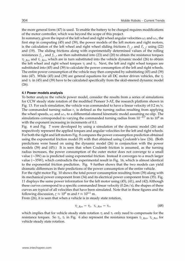
To better analyze the vehicle power model, consider the results from a series of simulationsfor CCW steady state rotation of the modified Pioneer 3-AT, the research platform shown inFig. 13. For each simulation, the vehicle was commanded to have a linear velocity of 0.2 m/s.The commanded turning radius rc is defined as the turning radius resulting from applyingthe wheel speeds, ωl and ωr, to a differential-steered kinematic model assuming no slip. Thesimulations corresponded to varying the commanded turning radius from 10−0.7 m to 104 mwith the exponent increasing in increments of 0.1.Fig. 6 and Fig. 7 were developed by using a simulation of the dynamic model (26) andrespectively represent the applied torques and angular velocities for the left and right wheels.For both the right and left motors Fig. 8 compares the power consumption prediction obtainedusing the exponential friction model (9) with that obtained using Coulomb’s law (24). (Bothpredictions were based on using the dynamic model (26) in conjunction with the powermodels (39) and (45).) It is seen that when Coulomb friction is assumed, as the turningradius increases, the power consumption of the outer motor does not converge to a smallvalue (∼3W) as is predicted using exponential friction. Instead it converges to a much largervalue (∼35W), which contradicts the experimental result in Fig. 16, which is almost identicalto the exponential friction prediction. Fig. 9 further shows that the two models can yielddramatic differences in their predictions of the power consumption of the entire vehicle.For the right motor Fig. 10 shows the total power consumption resulting from (39) along withits mechanical power component from (34) and its electrical power component from (35). Fig.11 displays the same power information for the left motor using (45), (41), and (42).Althoughthese curves correspond to a specific commanded linear velocity (0.2m/s), the shapes of thesecurves are typical of all velocities that have been simulated. Note that in these figures and thefollowing discussion, r ≈ 100 m and r ≈ 101.1 m.From (26), it is seen that when a vehicle is in steady state rotation,

τl_Res = τl , τr_Res = τr, (48)

which implies that for vehicle steady state rotation τl and τr only need to compensate for theresistance torques. So τl , τr in Fig. 6 also represent the resistance torques τl_Res, τr_Res forvehicle steady state rotation.


www.intechopen.com


Below, Fig. 6, Fig. 7 and Fig. 8 are used to analyze the current, voltage, and powerconsumption of each motor in greater detail. Particular attention is given to the inner (left)motor since it sometimes generates power.

Fig. 6. Steady-state, inner and outer wheel torques vs. commanded turning radius, obtainedvia simulation of the dynamic model, for a commanded linear velocity of 0.2 m/s on the labvinyl surface.

Fig. 7. Steady-state, inner and outer wheel angular velocities vs. commanded turning radius,obtained via simulation of the dynamic model for the conditions of Fig. 6.

Analysis of the Vehicle’s Outer (Right) SideFig. 6, Fig. 7 and Fig. 8 show that τr, ωr and Pr are always positive. From (36) and (33), itfollows that ir and Ur are also positive. Therefore, for the right side of the vehicle,

ir > 0, Ur > 0, Pr > 0, (49)

which implies that the outer motor always consumes power. The direction of current flow,and the voltage of the motor controller, motor resistance and motor have the same signs as inFig. 5.


www.intechopen.com


Fig. 8. Power prediction for the inner and outer motors vs. commanded turning radius usingexponential friction model (9) and Coulomb’s law.

Fig. 9. Power prediction for the whole vehicle corresponding to Fig. 8 using exponentialfriction model (9) and Coulomb’s law.

For the outer side of vehicle Fig. 10 shows that the mechanical power consumption andelectrical power consumption are nearly equal for each turning radius2. (As discussedafter (32), only the mechanical power is converted into motion while the electrical powerconsumption is dissipated (or wasted) as heat.) In this case, the power source is alwaysthe battery operating through the motor controller,3 while the motor shaft motion consumesmechanical power and the motor electrical resistance consumes electrical power. Referring to(47),

σ(Pr) = Pr, (50)

2 As the motor electrical resistance decreases, the electrical power consumption will be smaller than themechanical power consumption.

3 Some of the battery’s power is dissipated as heat in the motor controller’s resistance. See Fig. 5


www.intechopen.com


Fig. 10. Outer motor power comparison: outer total power consumption, outer mechanicalpower consumption and outer electrical power consumption, obtained via simulation of thedynamic model for the conditions of Fig. 6.

Fig. 11. Inner motor power comparison: inner total power consumption, inner mechanicalpower consumption and inner electrical power consumption, obtained via simulation of thedynamic model for the conditions of Fig. 6.

where Pr is given by (39).Analysis of the Vehicle’s Inner (Left) SideFig. 6 shows that τl can be either positive or negative, Fig. 7 shows that ωl is positive, whileFig. 8 shows that Pl can be either positive or negative. The signs of τl and Pl depend onwhether the commanded turning radius rc is in one of three regions: 1) rc ≥ r, 2) r < rc < r,and 3) rc ≤ r. These three cases are now analyzed.Case 1 (rc ≥ r, Pl > 0): Fig. 6, Fig. 7 and Fig. 8 show that τl > 0, ωl > 0 and Pl > 0. From (43)and (40), it follows il > 0, Ul > 0. Therefore, for the left side of the vehicle in this case,

il > 0, Ul > 0, Pl > 0, (51)


www.intechopen.com


which implies the left motor consumes power. The direction of the motor current flow andvoltage are as shown in Fig. 5.Fig. 11 shows that for each commanded turning radius rc satisfying rc ≥ r the total motorpower consumption is dominated by the mechanical power consumption although there is asmall amount of electrical power consumption. In this case, the power source is the motorcontroller system, while the motor shaft motion consumes mechanical power and the motorelectrical resistance consumes electrical power. Referring to (47),

σ(Pl) = Pl , (52)

where Pl is given by (45).Case 2 (r < rc < r, Pl < 0): Fig. 6, Fig. 7 and Fig. 8 show that τl < 0, ωl > 0 and Pl < 0. From(43) and (40), it follows il < 0, Ul > 0. Therefore, for the left side of the vehicle in this case,

il < 0, Ul > 0, Pl < 0, (53)

which implies that the left motor generates power. In Fig. 5 the direction of il and the voltagedrop across Re are reversed, while the motor controller voltage Ul and that of the motor remainas shown.Fig. 11 shows that for each commanded turning radius rc satisfying r < rc < r the mechanicalpower consumption is negative, and hence the motor shaft motion does not consume powerbut on the contrary generates power from the terrain. This is because when the vehicle rotates,the outer wheel drags the inner wheel through the vehicle body Morales et al. (2009), whichleads to the backward sliding friction for the inner wheel and the generation of power for theinner motor from terrain. Since the mechanically generated power is larger than the electricalpower consumption, there is a net power generation that is consumed by the motor controllersystem. In this case, the power source is the motor shaft, while the motor electrical resistanceand the motor controller system consume power. Referring to (47),

σ(Pl) = 0. (54)

Case 3 (rc ≤ r, Pl > 0): Fig. 6, Fig. 7 and Fig. 8 show that τl < 0, ωl > 0 and Pl > 0. From (43)and (40), it follows il < 0, Ul < 0. Therefore, for the left side of the vehicle in this case,

il < 0, Ul < 0, Pl > 0, (55)

which implies that the left motor consumes power. In Fig. 5 the direction of il , the voltagedrop across the Re and the motor controller voltage Ul are reversed, while the voltage sign ofthe motor remains the same.Fig. 11 shows for each commanded turning radius rc satisfying rc ≤ r the mechanicalpower consumption is negative, which means, as in Case 2, the motor shaft motion doesnot consume power but generates power from terrain. However, unlike Case 2, the generatedmechanical power is smaller than the electrical power consumption. Hence, there is a netpower consumption and the motor controller system still has to supply power. In this case, thepower sources are the motor shaft and the motor controller system, while the motor electricalresistance consumes power. Referring to (47),

σ(Pl) = Pl , (56)

where Pl is given by (45).


www.intechopen.com


Analysis of the Power Consumption of the Entire VehicleThe overall power consumption of the vehicle is due to the power consumption of both theinner and outer motors and is shown in Fig. 8. Fig. 12 shows the percentage of the overallpower consumption of the vehicle due to mechanical power consumption and electrical powerconsumption. It is of interest to note that when rc ≥ r, the mechanical power consumptionis dominant, while as rc decreases in value from r the electrical heat dissipation eventuallydominates. This indicates that in motion planning, as might be expected, it is more energyefficient to plan for trajectories with large turning radii.

Fig. 12. Mechanical power and electrical power consumption percentages vs. commandedturning radius, obtained via simulation of the dynamic model, for the conditions of Fig. 6.

In summary, analysis of the power models of the right and left motors reveal the interestingphenomenon that for vehicle steady state rotation while the outer motor always consumespower, as the vehicle turning radius decreases, the inner motor first consumes, then generatesand finally consumes power again. Since Fig. 8 is generated using the the power model (45),the model enables prediction of the two transition turning radii r and r.

5. Experimental results

This section presents the experiment and simulation results to verify the proposed dynamicmodels and power models in this chapter.The experimental platform is the modified Pioneer 3-AT shown in Fig. 13. The original,nontransparent, speed controller from the company was replaced by a PID controller andmotor controller. PC104 boards replaced the original control system boards that came with thevehicle. Two current sensors were mounted on each side of the vehicle to provide real timemeasurement of the motors’ currents. It was modified to run on the QNX realtime operatingsystem with a control sampling rate of 1KHz. The mobile robot can be commanded with alinear velocity and turning radius.


www.intechopen.com


Fig. 13. Modified Pioneer 3-AT

5.1 Steady state rotation for different turning radii

In this subsection, 2D steady state rotation results for different turning radii are presented. Fora vehicle commanded linear velocity of 0.2m/s and turning radius changing from 10−0.7 m to104 m, Fig. 14 shows the experimental and simulation wheel angular velocity vs. commandedradius, Fig. 15 shows the experimental and simulation applied torques vs. commanded radiusand Fig. 16 shows the experimental and simulated power consumption vs. commandedradius. In all figures there is good correspondence between the experimental and simulatedresults. If shear stress is not a function of shear displacement, but instead takes on a maximumvalue when there is a small relative movement between wheel and terrain, the left and rightmotor torques should be constant for different commanded turning radii, a phenomenon notseen in Fig. 15. Instead this figure shows the magnitudes of both the left and right torquesreduce as the commanded turning radius increases. The same trend is found in Wong (2001);Wong & Chiang (2001). Note that the three cases of inner motor power consumption areobserved in the experimental results of Fig. 16.

5.2 Circular movement with motor power saturation

In terms of motion planning one advantage of using the separate motor power models (39)and (45) instead of relying completely on the entire vehicle power model (47) is that theseparate models enable more accurate predictions of vehicle velocity when an individualmotor experiences power saturation. For a given trajectory it is possible for the entire vehiclepower consumption required to achieve that trajectory to be below the total power that canbe provided by the motor drive systems, but the power consumption required for one of themotors to be above the power limitations of that motor’s drive system. In this case the desiredtrajectory cannot be achieved.For the modified Pioneer 3-AT of Fig. 13, the maximum linear velocity is 0.93 m/s. The powerlimitation for each side of the motor drive system is 51 w, and total power limitation is 102w. Fig. 17 was generated using (39) and (45) and shows the power requirements for the innerand outer motors vs. commanded turning radius when the vehicle has a linear velocity of 0.7m/s. It also shows a line corresponding to the 51 w power limitation of each of the motordrive systems.For a vehicle commanded linear velocity of 0.7 m/s and turning radius of 1.2 m, the predictedinner and outer motor power requirements for a commanded turning radius of 1.2 m aremarked using square symbols in Fig. 17. It is seen that the outer motor power consumption is


www.intechopen.com


Fig. 14. Vehicle inner and outer wheel angular velocity comparison during steady-state CCWrotation for different commanded turning radii on the lab vinyl surface when thecommanded linear velocity is 0.2 m/s.

Fig. 15. Vehicle inner and outer wheel applied torque comparison corresponding to Fig. 14

approximately 58 w, which is above the 51 w power limitation, which means this velocity andradius combination cannot be achieved. However, the total power requirement in this case isalso equal to 58 w. This power requirement is well below the 102 w limitation for the entirevehicle, showing the importance of estimating the power consumption of each individualmotor. It is seen that as predicted by the power model for the outer wheel that this wheelwas unable to achieve the desired vehicle due to the power limitation of the motor drivesystem. Fig. 18 compares the experimental, simulation and commanded angular velocity forthe inner and outer wheels. Fig. 19 shows the experimental and simulation applied torques vs.


www.intechopen.com


Fig. 16. Vehicle inner and outer wheel power comparison comparison corresponding to Fig.14.

commanded radius and Fig. 20 shows the experimental and simulated power consumptionvs. commanded radius.

Fig. 17. Power limitation for each side of vehicle, and vehicle inner and outer wheel powerprediction during steady-state CCW rotation for different commanded turning radii on thelab vinyl surface when the commanded linear velocity is 0.7 m/s

5.3 Curvilinear movement

In this subsection, the model is to be tested for general 2D curvilinear motion. The vehiclewas commanded to move in lemniscate trajectory, which required it to have modest linearand angular accelerations. Fig. 21 shows one complete cycle lemniscate trajectory along withthe partial lemniscate trajectory used in the experiment.


www.intechopen.com


Fig. 18. Experiment, simulation and commanded angular velocity comparison for inner andouter wheels for 2D circular movement on the lab vinyl surface when the commanded radiusis 1.2 m and the commanded linear velocity is 0.7 m/s.

Fig. 19. Vehicle inner and outer wheels torque comparison corresponding to Fig. 18.

In Fig. 21, the lemniscate trajectory is governed by,

X(t) =9 cos( t

50 )

1 + sin2( t50 )

, (57)

Y(t) =27 sin( t

50 ) cos( t50 )

1 + sin2( t50 )

, (58)

where t is the time, and (X(t), Y(t)) is the position in global coordinates. The vehicle wasfirst commanded to go straight with an acceleration of 1 m/s2 to achieve the initial enteringvelocity 0.54 m/s of the lemniscate trajectory in Fig. 21 within 3 seconds. Then it wascommanded to follow the desired trajectory in Fig. 21 with changing linear velocity and


www.intechopen.com


Fig. 20. Vehicle inner and outer wheels power comparison corresponding to Fig. 18.

Fig. 21. Partial and whole lemniscate trajectories

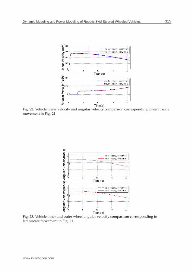
turning radius for another 18 seconds. The linear acceleration changes in the range [0 0.02]m/s2.Fig. 22, Fig. 23 and Fig. 24 show the experimental and simulation comparisons for the vehiclelinear and angular velocity, the inner and outer wheel angular velocity, and the inner andouter wheel applied torque. Fig. 25 shows the corresponding power comparison for the innerand outer part of the vehicle. These results reveal that if the vehicle turns with continuallychanging linear and angular accelerations of limited magnitude, the dynamic models andpower models are still capable of providing high fidelity predictions for both the inner andouter part of the vehicle. Fig. 25 also shows during the lemniscate traversal the inner motorgradually changes from consuming power to generating power while the outer motor alwaysconsumes power. The transition time for the inner motor can also be predicted from the motorpower model (45).


www.intechopen.com


Fig. 22. Vehicle linear velocity and angular velocity comparison corresponding to lemniscatemovement in Fig. 21

Fig. 23. Vehicle inner and outer wheel angular velocity comparison corresponding tolemniscate movement in Fig. 21


www.intechopen.com


Fig. 24. Vehicle inner and outer wheel torque comparison corresponding to lemniscatemovement in Fig. 21

Fig. 25. Vehicle inner and outer wheel power comparison corresponding to lemniscatemovement in Fig. 21


www.intechopen.com


6. References

Caracciolo, L., Luca, A. D. & Iannitti, S. (1999). Trajectory tracking control of a four-wheeldifferentially driven mobile robot, Proceedings of the IEEE International Conference onRobotics and Automation, Detroit, MI, pp. 2632–2638.

Economou, J., Colyer, R., Tsourdos, A. & White, B. (2002). Fuzzy logic approaches for wheeledskid-steer vehicle, Vehicular Technology Conference, pp. 990–994.

Endo, D., Okada, Y., Nagatani, K. & Yoshida, K. (2007). Path following control for trackedvehicles based slip-compensation odometry, Proceedings of the IEEE InternationalConference on Intelligent Robots and Systems, pp. 2871–2876.

Golconda, S. (2005). Steering control for a skid-steered autonomous ground vehicle at varying speed,Master’s thesis, University of Louisiana at Lafayette.

Howard, T. M. & Kelly, A. (2007). Optimal rough terrain trajectory generation for wheeledmobile robots, International Journal of Robotics Research pp. 141–166.

Kim, C. & Kim, B. K. (2007). Minimum-energy translational trajectory generationfor differential-driven wheeled mobile robots, Journal of Intelligent Robot Systempp. 367–383.

Kozlowski, K. & Pazderski, D. (2004). Modeling and control of a 4-wheel skid-steering mobilerobot, International Journal of Mathematics and Computer Science pp. 477–496.

Mandow, A., Martlłnez, J. L., Morales, J., Blanco, J.-L., Garclła-Cerezo, A. & Gonzalez, J.(2007). Experimental kinematics for wheeled skid-steer mobile robots, Proceedingsof the International Conference on Intelligent Robots and Systems, San Diego, CA,pp. 1222–1227.

Martinez, J., Mandow, A., Morales, J., Pedraza, S. & Garcia-Cerezo, A. (2005). Approximatingkinematics for tracked mobile robots, International Journal of Robotics Researchpp. 867–878.

Moosavian, S. A. A. & Kalantari, A. (2008). Experimental slip estimation for exact kinematicsmodeling and control of a tracked mobile robot, Proceedings of the InternationalConference on Intelligent Robots and Systems, Nice, France, pp. 95–100.

Morales, J., Martinez, J. L., Mandow, A., Garcia-Cerezo, A., Gomez-Gabriel, J. & Pedraza, S.(2006). Power anlysis for a skid-steered tracked mobile robot, Proceedings of the IEEEInternational Conference on Mechatronics, pp. 420–425.

Morales, J., Martinez, J. L., Mandow, A., Garcia-Cerezo, A. J. & Pedraza, S. (2009). Powerconsumption modeling of skid-steer tracked mobile robots on rigid terrain, IEEETransactions on Robotics pp. 1098–1108.

Nagatani, K., Endo, D. & Yoshida, K. (2007). Improvement of the odometry accuracyof a crawler vehicle with consideration of slippage, Proceedings of the InternationalConference on Robotics and Automation, Rome, Italy, pp. 2752–2757.

O. Chuy, J., E. Collins, J., Yu, W. & Ordonez, C. (2009). Power modeling of a skid steeredwheeled robotic ground vehicle, Proceedings of the IEEE International Conference onRobotics and Automation, Kobe, Japan.

Petrov, P., de Lafontaine, J., Bigras, P. & Tetreault, M. (2000). Lateral control of a skid-steeringmining vehicle, Proceedings of the International Conference on Intelligent Robots andSystems, Takamatsu, Japan, pp. 1804–1809.

Rizzoni, G. (2000). Principles and Applications of Electrical Engineering, McGraw-Hill.Shamah, B., Wagner, M. D., Moorehead, S., Teza, J., Wettergreen, D. & Whittaker, W. R. L.

(2001). Steering and control of a passively articulated robot, SPIE, Sensor Fusion andDecentralized Control in Robotic Systems IV, Vol. 4571.


www.intechopen.com


Siegwart, R. & Nourbakhsh, I. R. (2005). Introduction to Mobile Robotics, MIT Press, Cambridge,MA.

Song, X., Song, Z., Senevirante, L. & Althoefer, K. (2008). Optical flow-based slip and velocityestimation technique for unmanned skid-steered vehicles, pp. 101–106.

Song, Z., Zweiri, Y. H. & Seneviratne, L. D. (2006). Non-linear observer for slip estimation ofskid-steering vehicles, Proceedings of the IEEE International Conference on Robotics andAutomation, Orlando, Fl, pp. 1499–1504.

Wang, H., Zhang, J., Yi, J., Song, D., Jayasuriya, S. & Liu, J. (2009). Modeling andmotion stability analysis of skid-steered mobile robots, Proceedings of the InternationalConference on Robotics and Automation, Kobe, Japan, pp. 4112– 4117.

Wong, J. Y. (2001). Theory of Ground Vehicle, 3rd edn, John Wiley & Sons, Inc.Wong, J. Y. & Chiang, C. F. (2001). A general theory for skid steering of tracked vehicles on

firm ground, Proceedings of the Institution of Mechanical Engineers, Part D, Journal ofAutomotive Engineerings pp. 343–355.

Yi, J., Song, D., Zhang, J. & Goodwin, Z. (2007). Adaptive trajectory tracking control ofskid-steered mobile robots, Proceedings of the IEEE International Conference on Roboticsand Automation, Roma, Italy, pp. 2605–2610.

Yi, J., Zhang, J., Song, D. & Jayasuriya, S. (2007). IMU-based localization and slip estimation forskid-steered mobile robot, Proceedings of the IEEE International Conference on IntelligentRobots and Systems, San Diego, CA, pp. 2845–2849.

Yu, W., Chuy, O., Collins, E. G. & Hollis, P. (2010). Analysis and experimental verification fordynamic modeling of a skid-steered wheeled vehicle, IEEE Transactions on Roboticspp. 440–453.

Zhang, Y., Hong, D., Chung, J. H. & Velinsky, S. A. (1998). Dynamic model based robusttracking control of a differentially steered wheeled mobile robot, Proceedings of TheAmerican Control Conference, Philadelphia, PA, pp. 850–855.


www.intechopen.com

Mobile Robots - Current TrendsEdited by Dr. Zoran Gacovski

ISBN 978-953-307-716-1Hard cover, 402 pagesPublisher InTechPublished online 26, October, 2011Published in print edition October, 2011

InTech EuropeUniversity Campus STeP Ri Slavka Krautzeka 83/A 51000 Rijeka, Croatia Phone: +385 (51) 770 447 Fax: +385 (51) 686 166www.intechopen.com

InTech ChinaUnit 405, Office Block, Hotel Equatorial Shanghai No.65, Yan An Road (West), Shanghai, 200040, China

Phone: +86-21-62489820 Fax: +86-21-62489821

This book consists of 18 chapters divided in four sections: Robots for Educational Purposes, Health-Care andMedical Robots, Hardware - State of the Art, and Localization and Navigation. In the first section, there arefour chapters covering autonomous mobile robot Emmy III, KCLBOT - mobile nonholonomic robot, andgeneral overview of educational mobile robots. In the second section, the following themes are covered:walking support robots, control system for wheelchairs, leg-wheel mechanism as a mobile platform, micromobile robot for abdominal use, and the influence of the robot size in the psychological treatment. In the thirdsection, there are chapters about I2C bus system, vertical displacement service robots, quadruped robots -kinematics and dynamics model and Epi.q (hybrid) robots. Finally, in the last section, the following topics arecovered: skid-steered vehicles, robotic exploration (new place recognition), omnidirectional mobile robots, ball-wheel mobile robots, and planetary wheeled mobile robots.

How to referenceIn order to correctly reference this scholarly work, feel free to copy and paste the following:

Wei Yu, Emmanuel Collins and Oscar Chuy (2011). Dynamic Modeling and Power Modeling of Robotic Skid-Steered Wheeled Vehicles, Mobile Robots - Current Trends, Dr. Zoran Gacovski (Ed.), ISBN: 978-953-307-716-1, InTech, Available from: http://www.intechopen.com/books/mobile-robots-current-trends/dynamic-modeling-and-power-modeling-of-robotic-skid-steered-wheeled-vehicles

Documents

Dynamic Modeling and Power Modeling of Robotic Skid ...cdn.intechopen.com/pdfs/22305.pdf · Section 1 is the introduction. Section 2 presents ... model of a skid-steered vehicle was