Dynamic graph-based search in unknown environments

Journal of Discrete Algorithms 12 (2012) 2–13

Contents lists available at ScienceDirect

Journal of Discrete Algorithms

www.elsevier.com/locate/jda

Dynamic graph-based search in unknown environments

Paul S. Haynes ∗, Lyuba Alboul ∗∗, Jacques Penders

Centre for Automation and Robotics Research, Sheffield Hallam University, City Campus, Howard Street, S1 1WB, UK

a r t i c l e i n f o a b s t r a c t

Article history:Available online 6 July 2011

Keywords:Dynamic searchGraph theoryTeam roboticsMulti-robot localisation

A novel graph-based approach to search in unknown environments is presented. A virtualgeometric structure is imposed on the environment represented in computer memory by agraph. Algorithms use this representation to coordinate a team of robots (or entities). Localdiscovery of environmental features cause dynamic expansion of the graph resulting inglobal exploration of the unknown environment. The algorithm is shown to have O (k · nH )

time complexity, where nH is the number of vertices of the discovered environment and1 � k < nH . A maximum bound on the length of the resulting walk Ω is given.

© 2011 Elsevier B.V. All rights reserved.

1. Introduction

The method presented in this paper stems from the research in multi-robot systems within the remits of the recentlycompleted GUARDIANS project.1 Autonomous mobile robotics, in particular collective and cooperative robotics, has gained alot of attention recently.

Multi-robot systems pose new challenging problems such as cooperative perception and localisation, cooperative taskplanning and execution, team navigation behaviors, robot interactions among themselves and with humans, cooperativelearning, and communication.

There have been some significant advances in tackling the aforementioned problems, often based, however, on empiricalapproaches. They are either driven by informal expert knowledge, or by resource-intensive trial-and-error processes [7].

There is a demanding need for formalization of methodologies and theoretical frameworks capable of providing solutionsto general classes of problems specific to multi-robot systems.

In this paper such a framework, based on the concept of [1], is proposed for the problem of global self-localisation ofmulti-robot teams, without a priori information about the environment.

The problem of self-localisation is central in robotics, and is particularly difficult in unknown indoor environments wheresuch position systems as GPS are unavailable.

It is directly related to the famous SLAM problem of a robot simultaneously localising and building a map of the environ-ment. This problem has been studied extensively in the robotics literature, focusing mostly on a single robot. Conceptually,the SLAM problem for a single robot in 2D is considered to be solved, but in practice it may still encounter difficulties,even outdoors, in urban areas or forests. SLAM approaches are mainly probabilistic in their nature due to the uncertainty ofacquired information. Data association methods used in SLAM require significant computation in real-life implementations,and contribute to increased complexity [3].

The problem of multi-robot localisation and encountered difficulties has not yet been fully researched [5]. A multi-robotteam, by definition, represents a sensor network. An important aspect of a multiple robotic system, as opposed to a single

* Corresponding author.

** Principal corresponding author.E-mail addresses: [email protected] (P.S. Haynes), [email protected] (L. Alboul), [email protected] (J. Penders).

1Guardians, Group of Unmanned Assistant Robots Deployed in Aggregative Navigation supported by Scent Detection, EU FP6 ICT 045269.

1570-8667/$ – see front matter © 2011 Elsevier B.V. All rights reserved.doi:10.1016/j.jda.2011.06.004

http://dx.doi.org/10.1016/j.jda.2011.06.004

http://www.ScienceDirect.com/

http://www.elsevier.com/locate/jda

mailto:[email protected]



http://dx.doi.org/10.1016/j.jda.2011.06.004

P.S. Haynes et al. / Journal of Discrete Algorithms 12 (2012) 2–13 3

robot, is the richness of available information. In a cooperative multi-robot team, robots obtain information from their ownsensors as well as other robots. This information can be of various types: perceptual (data from lasers, various distributedcameras) as well as non-perceptual (symbolic information, directions, and commands, obtained from other robots or adatabase). Therefore, such plethora of information should be taken into account.

In the last decade, several works have appeared that tackle the problem of cooperative multi-robot localisation. Whereassome approaches still consider the problem within the SLAM framework, by treating the problem of multi-robot localisationas a Multi-SLAM problem [6], others, while still using probabilistic methods, attempt to take into consideration robots aslandmarks themselves [8]. Another trend is based on robot distribution on site, which can work well if the group of robotsis large and communication between them is robust [10].

A promising mathematical tool to characterize a multi-robot system is a graph. Indeed, the problem of coordination inmulti-robot systems can be characterized naturally by a finite representation of the configuration space using Graph Theory.Vertices represent robots with resources limited by sensors, control design, and computational power. Edges are virtualentities describing local interactions and can support information flow between vertices/robots. If other sensor devicesare present in the environment they can be added to the sensor robot networks. Graph theory facilitates analysis of theinterplay between the communications network and robot dynamics, and to choose strategies for information exchangewhich mitigate these effects.

Graph-theoretical approaches have been increasingly used for building and analyzing communication and sensor net-works [11].

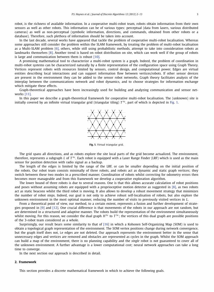
In this paper we describe a graph-theoretical framework for cooperative multi-robot localisation. The (unknown) site isinitially covered by an infinite virtual triangular grid (triangular tiling) T ∞ , part of which is depicted in Fig. 1.

Fig. 1. Virtual triangular grid.

The grid spans all directions, and as robots explore the site local parts of the grid become actualized. The environment,therefore, represents a subgraph L of T ∞ . Each robot is equipped with a Laser Range Finder (LRF) which is used as the mainsensor for position detection with radio signal as a backup.

The length of the edges is limited by the range of the LRF, or can be smaller depending on the initial position ofthe robots. Our robot team consists minimally of three robots, and robots act as dynamic and static graph vertices; theyswitch between these two modes in a prescribed manner. Coordination of robots whilst correcting for odometry errors thenbecomes more manageable and from this framework we develop a cooperative exploration algorithm.

The lower bound of three robots is due to several reasons. One is that this allows accurate calculation of robot positionsand poses without assuming robots are equipped with a proprioceptive motion detector as suggested in [8], as two robotsact as static beacons whilst the third robot is moving. It also allows to develop a robust movement strategy that minimizesthe number of robot steps. Indeed, our goal is not only to achieve robust self-localisation of robots, but also explore theunknown environment in the most optimal manner, reducing the number of visits to previously visited vertices in L.

From a theoretical point of view, our method, to a certain extent, represents a fusion and further development of strate-gies proposed in [9] and [12]. One crucial difference is that movements of the robots in our approach are not random, butare determined in a structured and adaptive manner. The robots build the representation of the environment simultaneouslywhilst moving. For this reason, we consider the dual graph H∞ to T ∞; the vertices of this dual graph are possible positionsof the 3-robot team considered as a whole.

Surprisingly, our result bears some similarity to that of [16] in which a Kohonen Self-Organizing Map (SOM) is used toobtain a topological graph representation of the environment. The SOM vertex positions change during network convergence,but the graph itself does not, i.e edges are not deleted. Our approach represents the environment better in the sense thatunnecessary edges and vertices are removed and obstacles are represented as cycles in the graph. Whilst the SOM approachcan build a map of the environment, there is no planning capability and the single robot is not guaranteed to cover all ofthe unknown environment. A further advantage is a lower computational cost; neural network approaches can take a longtime to converge.

In the next section our approach is described in detail.

2. Framework

This section provides a discrete mathematical framework in which to achieve the following goals.

4 P.S. Haynes et al. / Journal of Discrete Algorithms 12 (2012) 2–13

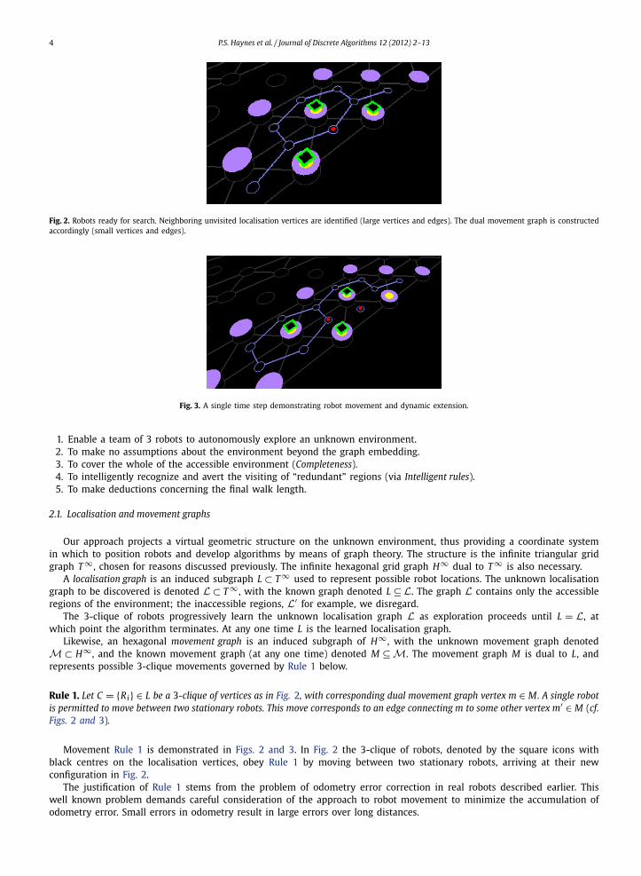
Fig. 2. Robots ready for search. Neighboring unvisited localisation vertices are identified (large vertices and edges). The dual movement graph is constructedaccordingly (small vertices and edges).

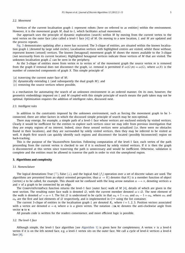
Fig. 3. A single time step demonstrating robot movement and dynamic extension.

1. Enable a team of 3 robots to autonomously explore an unknown environment.2. To make no assumptions about the environment beyond the graph embedding.3. To cover the whole of the accessible environment (Completeness).4. To intelligently recognize and avert the visiting of “redundant” regions (via Intelligent rules).5. To make deductions concerning the final walk length.

2.1. Localisation and movement graphs

Our approach projects a virtual geometric structure on the unknown environment, thus providing a coordinate systemin which to position robots and develop algorithms by means of graph theory. The structure is the infinite triangular gridgraph T ∞ , chosen for reasons discussed previously. The infinite hexagonal grid graph H∞ dual to T ∞ is also necessary.

A localisation graph is an induced subgraph L ⊂ T ∞ used to represent possible robot locations. The unknown localisationgraph to be discovered is denoted L ⊂ T ∞ , with the known graph denoted L ⊆ L. The graph L contains only the accessibleregions of the environment; the inaccessible regions, L′ for example, we disregard.

The 3-clique of robots progressively learn the unknown localisation graph L as exploration proceeds until L = L, atwhich point the algorithm terminates. At any one time L is the learned localisation graph.

Likewise, an hexagonal movement graph is an induced subgraph of H∞ , with the unknown movement graph denotedM ⊂ H∞ , and the known movement graph (at any one time) denoted M ⊆ M. The movement graph M is dual to L, andrepresents possible 3-clique movements governed by Rule 1 below.

Rule 1. Let C = {Ri} ∈ L be a 3-clique of vertices as in Fig. 2, with corresponding dual movement graph vertex m ∈ M. A single robotis permitted to move between two stationary robots. This move corresponds to an edge connecting m to some other vertex m′ ∈ M (cf.Figs. 2 and 3).

Movement Rule 1 is demonstrated in Figs. 2 and 3. In Fig. 2 the 3-clique of robots, denoted by the square icons withblack centres on the localisation vertices, obey Rule 1 by moving between two stationary robots, arriving at their newconfiguration in Fig. 2.

The justification of Rule 1 stems from the problem of odometry error correction in real robots described earlier. Thiswell known problem demands careful consideration of the approach to robot movement to minimize the accumulation ofodometry error. Small errors in odometry result in large errors over long distances.


2.2. Movement

Vertices of the current localisation graph L represent robots (here on referred to as entities) within the environment.However, it is the movement graph M , dual to L, which facilitates actual movement.

Our approach uses the principle of dynamic exploration (search) within M by moving from the current vertex to thenext vertex on the outer face (also called a level-1 face [4]) of M . On moving to a new location, L and M are updated andthe process repeats.

Fig. 3 demonstrates updating after a move has occurred. The 3-clique of entities, are situated within the known localisa-tion graph L (denoted by large solid circles). Localisation vertices with highlighted centres are visited, whilst those without,represent known (sensed) vertices. The known (hexagonal) movement graph M shows the moves available to the 3-clique(not necessarily from its current location). Highlighted hexagonal vertices indicate those vertices of M that are visited. Theunknown localisation graph L can be seen in the periphery.

As the 3-clique of entities move from vertex m to vertex m′ of the movement graph the source vertex m is removedfrom the graph if removal does not disconnect the graph, i.e. removal is permitted if ω(G\m) = ω(G), where ω(X) is thenumber of connected components of graph X . This simple principle of

(a) traversing the current outer face of M;(b) dynamically extending L (and subsequently the dual graph M); and(c) removing the source vertices where possible,

is a mechanism for automating the search of an unknown environment in an ordered manner. On its own, however, thegeometric embeddings imposed on L and M coupled with this simple principle of search means the path taken may not beoptimal. Optimization requires the addition of intelligent rules, discussed next.

2.3. Intelligent rules

In addition to the constraints imposed by the unknown environment, such as forcing the movement graph to be 1-connected, there are other factors in which the discussed simple principle of search may be non-optimal.

There may emerge, for example, a simple path of a level-1 face whose vertices are enclosed entirely by visited vertices.Clearly it would be inefficient for the entities to explore such vertices since we may infer from previous investigation thatthey are empty regions of no interest. Indeed, since these sensed vertices were actualized (i.e. there were no obstaclesfound in their locations), and they are surrounded by solely visited vertices, then they may be inferred to be visited aswell. A depth first search can quickly identify such regions and disconnect the located (possibly biconnected) region onback-tracking.

This is the purpose of the ValidatePath function. Following computation of the level-1 face, each vertex of the pathproceeding from the current vertex is checked to see if it is enclosed by solely visited vertices. If it is then the graphis disconnected at this vertex since traversing the path is unnecessary and would be inefficient. Otherwise, validation iscomplete and the entities must be allowed to traverse the path in order to visit the unexplored region.

3. Algorithms and complexity

3.1. Nomenclature

The logical denotations True (�), False (⊥), and the logical And (∧

) operation over a set of discrete values are used. Thealgorithms are presented from an object oriented perspective, thus a → F() denotes that F() is a member function of object(vertex) a to be called, for example. This should not be confused with the long arrow notation u −→ v , denoting vertices uand v of a graph to be connected by an edge.

The ComputeOuterFace function returns the level-1 face (outer face) walk of M [4], details of which are given in thenext section. The resulting outer face walk is denoted Ω , with the current member denoted ω ∈ Ω . The next element ofthe walk is denoted ω′ = ω + 1. The list Ω is understood to be cyclic in that ωn + 1 = ω1 and ω1 − 1 = ωn , where ω1 andωn are the first and last elements of Ω respectively, and is implemented in C++ using the list container.

The current 3-clique of entities in the localisation graph L are denoted Ri , where i = 1,2,3. Position vectors associatedwith a vertex are denoted a → c, where a is a given vertex. The notation � (u,v) denotes the anti-clockwise angle fromvector u to v.

All pseudo code is written for the readers convenience, and more efficient logic is possible.

3.2. The level-1 face

Although simple, the level-1 face algorithm (see Algorithm 1) is given here for completeness. A vertex v is a level-kvertex if it is on the kth nested face, e.g. a level-1 vertex sits on the outer face. We call a cycle of level-k vertices a level-kface [4].


Algorithm 1 ComputeOuterFace(G)Computes the level-1 face of graph G.

1: Find left most vertex v ∈ G .2: Let u = (0,1)

3: Find argminw {� (u,−−→v w)|v −→ w}

4: Let s = −−→v w5: f = v6: while s �= u do7: f + w8: Let u = −−→w v, v = w9: Find argminw {� (u,

−−→v w)|v −→ w}10: end while11: return f

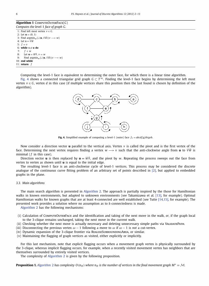
Computing the level-1 face is equivalent to determining the outer face, for which there is a linear time algorithm.Fig. 4 shows a connected triangular grid graph G ⊂ T ∞ . Finding the level-1 face begins by determining the left most

vertex v ∈ G , vertex d in this case (if multiple vertices share this position then the last found is chosen by definition of thealgorithm).

Fig. 4. Simplified example of computing a level-1 (outer) face f1 = abcdf g jihigeb.

Now consider a direction vector u parallel to the vertical axis. Vertex v is called the pivot and is the first vertex of theface. Determining the next vertex requires finding a vertex w −→ v such that the anti-clockwise angle from u to −−→v w isminimal ( f in this case).

Direction vector u is then replaced by u = −−→w v , and the pivot by w . Repeating the process sweeps out the face fromvertex to vertex as shown until u is equal to the initial edge.

The resulting level-1 face is an anti-clockwise cycle of level-1 vertices. This process may be considered the discreteanalogue of the continuous curve fitting problem of an arbitrary set of points described in [2], but applied to embeddedgraphs in the plane.

3.3. Main algorithms

The main search algorithm is presented in Algorithm 2. The approach is partially inspired by the those for Hamiltonianwalks in known environments, but adapted to unknown environments (see Takamizawa et al. [13], for example). OptimalHamiltonian walks for known graphs that are at least 4-connected are well established (see Tutte [14,15], for example). Thepresented work provides a solution where no assumption as to k-connectedness is made.

Algorithm 2 has the following mechanisms:

(i) Calculation of ComputeOuterFace and the identification and taking of the next move in the walk, or, if the graph localto the 3-clique remains unchanged, taking the next move in the current walk.

(ii) Checking whether the next move is actually necessary and deleting unnecessary simple paths via ValidatePath.(iii) Disconnecting the previous vertex ω − 1 following a move to ω if ω − 1 is not a cut-vertex.(iv) Dynamic expansion of the 3-clique frontier via RealiseSurroundingArea, or similar.(v) Maintaining the flagging of graph vertices as visited, either explicitly or implicitly.

For this last mechanism, note that explicit flagging occurs when a movement graph vertex is physically surrounded bythe 3-clique, whereas implicit flagging occurs, for example, when a recently visited movement vertex has neighbors that arethemselves surrounded by entirely visited vertices.

The complexity of Algorithm 2 is given by the following proposition.

Proposition 1. Algorithm 2 has complexity O (nH ) where nH is the number of vertices in the final movement graph M∗ = M.


Algorithm 2 DynamicSearch()Search unknown environment

1: if graph_altered then {If true, compute new outer face walk}2: ω′ ← ∅3: if Ω �= ∅ then {If a previous walk exists}4: ω′ ← ω + 1 {ω points to the next element in the walk}5: end if6: Ω ← (ω → ComputeOuterFace(·)) {Compute new walk}7: if ω′ �= ∅ then8: if there exists v ∈ Ω such that (v = ω) ∧ ((v + 1) = ω′) then {Find exact position in Ω if possible (should the local walk remain unchanged)}9: ω ← v {Set current position}

10: Exit at step 1511: end if12: end if13: Find ω′ ∈ Ω such that ω′ = ω {Since the local walk has changed, find any matching vertex}14: ω ← ω′15: end if16: if ω → ValidatePath(ω + 1) then {Check necessity of path}17: graph_altered ← � {Redundant paths have been removed}18: Restart from step 119: end if20: ω ← ω + 1 {Move to next vertex in walk}21: Find i ∈ {1,2,3} such that Ri �∈ (ω → S) {Determine entity to move}22: Ri ← (ω → S)\((ω − 1) → S) {Move the entity}23: r ← Ri {Remember which entity moved}24: r → visited ← � {Set it as visited}25: if h is not a cut-vertex then {Remove previously visited vertex?}26: Disconnect h from all neighbors.27: end if28: (ω → visited) ← ∧3

i=1 (Ri → visited)

29: graph_altered ← (RealiseSurroundingArea(r) > 0) {Update L and M}30: for all 3-cliques Ci ∈ L such that r ∈ Ci and

∧c∈Ci

(c → visited) do {Remove visited movement graph vertices v dual to Ci }31: Let v ∈ M be the hexagonal vertex dual to Ci .32: if v �= ω then {Do not consider current clique}33: if v connects to any other vertices then34: Disconnect those vertices connecting to v which are not cut-vertices.35: graph_altered = �36: end if37: end if38: end for39: for all connected neighbors s ∈ N(r) such that ¬(s → visited) do40: s → visited ← ∧

s′∈N(s)(s′ → visited) {s becomes visited if its surrounding vertices are visited}41: end for42: return

Proof. The first subroutine of Algorithm 2 is ComputeOuterFace which computes the level-1 face of the current movementgraph M . This is a simple O (n) time algorithm as discussed in Section 3.2.

Following computation of the level-1 face requires locating where in the new level face corresponds to the previouslocation in the previous level face so that we can take the next move. This takes O (|Ω|), where nH � |Ω| � 2nH .

Path validation and removing of unnecessary paths via ValidatePath takes O (nH ) time (see Proposition 2).The remaining subroutines remove remaining implicitly visited regions local to the 3-clique. Finally, by Proposition 3 (see

below), the RealiseSurroundingArea subroutine has complexity O (1). Summing gives an overall complexity of O (nH ). �Algorithm 2 makes use of the ValidatePath function (see Algorithm 3 and Recur, its related function), introduced in the

previous section, which has complexity given by the following proposition.

Proposition 2. Algorithm 3 has an upper bound complexity of O (nH ).

Proof. A level-1 face P ⊂ M has a maximum of nP < nH vertices. Since Algorithm 2 is effectively a depth first search of P ,its complexity is O (nP ), or a weaker condition states that for any path P Algorithm 3 has complexity O (nH ). �Algorithm 3 ValidatePath(p)

Searches for and removes unnecessary pathsavoid ← thisif p → Recur() then

Disconnect p from avoid.return �

end ifreturn ⊥


The RealiseSurrouondingArea function (see Algorithm 4), used by Algorithm 2, depends on the application at hand.A robotics setting would require this function to physically scan the surrounding area to determine which vertices to add tothe localisation graph L, and to connect vertices appropriately.

ValidatePath: Recur()

1: rtn ← �2: visited ← ∧

s′∈S (s′ → visited)

3: this → visited ← �4: if ¬ visited then5: return ⊥6: end if7: for all p ∈ N(this), p ∈ Ω such that p �= avoid of this vertex do8: if p has not yet been traversed by DFS then9: if (p → Recur()) then

10: Disconnect p from all its neighbors.11: else12: rtn ← ⊥13: end if14: end if15: end for16: return rtn

However, for simulation purposes an algorithm based on a known connected graph L is presented. Only those verticeson the periphery of the 3-clique within L are made available to the algorithms. Thus, RealiseSurroundingArea examinesthe unknown localisation graph L, with the entities only being aware of the vertices of the induced subgraph L ∈ L whichthey have previously visited, and the traversal boundary (i.e. unvisited yet sensed, or “known”, vertices).

Complexity of RealiseSurroundingArea is given by the following proposition, which, by the fixed graph embedding, islikely to be the case in practically all applications.

Fig. 5. Dynamic graph construction.

Proposition 3. Algorithm 4 has complexity O (1).

Proof. Algorithm 4 operates on induced subgraphs of the infinite triangular grid graph T ∞ , and the number of 3-cliquesabout vertex r is constant (cf. Fig. 6). Thus, there are a maximum of five such 3-cliques since there are six 3-cliquescontaining a single given vertex of the induced sub-graph and we disregard the current 3-clique since it is occupied. Theset P then has a maximum of 5 elements.

Fig. 6. Example of 3-clique formation centred on r, C = {{r23}, {r34}, {r45}, {r56}}. Here two possible cliques are missing.


Finally, each element s of P considers all elements t ∈ P proceeding s. Since there are a maximum of 5 elements in Pthis requires a maximum and constant number of 4+3+2 = 4(4+1)/2−1 = 10 operations. Therefore, the total complexityis O (1). �

Algorithm 4 RealiseSurroundingArea()Dynamically extend the graph

1: P ← ∅ + {(ω → c,ω)}2: r → known ← �3: for all 3-cliques Ci = {r,a,b} ∈ L where (¬(a → known)) ∧ (b → known) do4: v → c ← 1

3

∑c∈Ci

c → c {Make v ∈ M the dual vertex to Ci ∈ L}5: v → visited ← ∧

c∈Ci(c → visited)

6: v → S ← Ci

7: P ← P + {(v → c, v)}8: end for9: counter ← 0

10: for all elements s ∈ P do11: for all elements t ∈ P such that all t proceed s do12: if ‖(s → c) − (t → c)‖2 < 3/2 then {Is this a neighboring hexagonal vertex}13: if s � t and s has not been previously disconnected from t then14: Connect s to t . {Establish new connections (edges)}15: counter ← counter + 116: end if17: end if18: end for19: end for20: return counter

4. Analysis and discussion

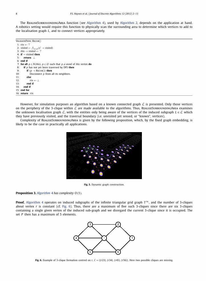
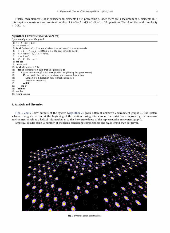
Figs. 5 and 7 show outputs of the system (Algorithm 2) given different unknown environment graphs L. The systemachieves the goals set out at the beginning of this section, taking into account the restrictions imposed by the unknownenvironment (such as a lack of information as to the k-connectedness of the representative movement graph).

Empirical results aside, a number of theorems concerning completeness and walk length may be proved.

Fig. 7. Dynamic graph construction.


4.1. Completeness

Completeness (briefly mentioned in Section 2) ensures the algorithm completely covers the unknown localisationgraph L.

Theorem 1 (Completeness). Let L be the localisation graph of the environment, initially unknown to the 3-clique of entities C = {Ri}whose dual vertex is m ∈ M. Then the final walk Ω∗ ∈ M produced by Algorithm 2 spans the entire graph L.

Proof. Consider the unknown localisation graph L and initial movement graph M (cf. Figs. 2 and 3, for example). WhereverL permits, each 3-clique of L instantiates a connected vertex m′ ∈ M of the movement graph. Moreover, on moving to a newmovement node, m′ say, where m −→ m′ , L is updated according to L. Moving from m to m′ will disconnect the two nodesif ω(M \ m) = ω(M), i.e. m is not a cut vertex. Thus, the mechanism of extension exists to instantiate and connect thosevertices having potential to exist, but which have not previously been disconnected. The proof is completed by induction.

By this mechanism of extension, there always exists a simple path P ∈ M of length l + 1, where P = mp1 p2 · · · pl , suchthat there exists q ∈ N(pl) unvisited, where N(pl) is the set of neighboring vertices of pl . The case for which l = 0 issimply the case for which one or more neighbors m′ of m are unvisited. If no such simple path exists then the algorithmis complete since, by definition, a path is only ever disconnected when m is a cut vertex rooting one or more biconnectedcomponents which are wholly visited or enclosed by wholly visited vertices. Thus, a simple path connecting to an unvisitedbiconnected component of the graph is never disconnected.

In the case where the next move of the movement graph M relative to the 3-clique is unaltered from the previous level-1 face walk, then the next vertex within the previously calculated level-1 face (ω′ = ω + 1) of Ω ∈ M is traversed. Traversalcontinues until an unvisited vertex is reached, in which case the graph is dynamically extended, and the outer face walk isrecalculated, thus completing the induction. �4.2. Walk length

The system deals with unknown environment exploration with no a priori knowledge of the search domain. Thus, deter-mining an exact upper bound length for the final walk Ω∗ is difficult since clearly this depends on the unknown.

However, in this section we present a logical argument which makes headway in understanding the walk length resultingfrom Algorithm 2. An upper bound is given on the length of the final walk Ω∗ .

To do this consideration of the key subroutines (mechanisms (i)–(v) listed in Section 3.3) of the algorithm is required.Let L∗ = L be the final localisation graph discovered by Algorithm 2. Then the final walk length, h(Ω∗), depends on the

features contained within L∗ which, of course, directly effects the final movement graph M∗ = M.Assuming we work with L∗ and M∗ for the moment, then by mechanisms (i), (iv), and (v) the algorithm, by definition

of the level-1 face algorithm, follows the boundary vertices of L∗ . In addition mechanism (iii) deletes the graph vertex of allprevious moves ω − 1 where possible, thus reducing (before dynamic expansion) the graph of available future moves.

This mechanism causes previously visited vertices to act as “walls” of the environment, thus the algorithm will not treadthese vertices on its next return unless doing so would allow access to one or more unvisited regions (such as biconnectedcomponents).

We can deduce that this leads to a “spiders-web”, or spiraling, approach to graph discovery until all available verticesbecome visited.

Additionally, however, the remaining mechanism (ii) implements an element of intelligence which makes spiraling moreefficient. During the course of the algorithm it may emerge that certain simple paths of the graph are surrounded entirelyby visited vertices. Clearly it would be inefficient to traverse such simple paths, and the mechanism identifies and removesthem using depth first search.

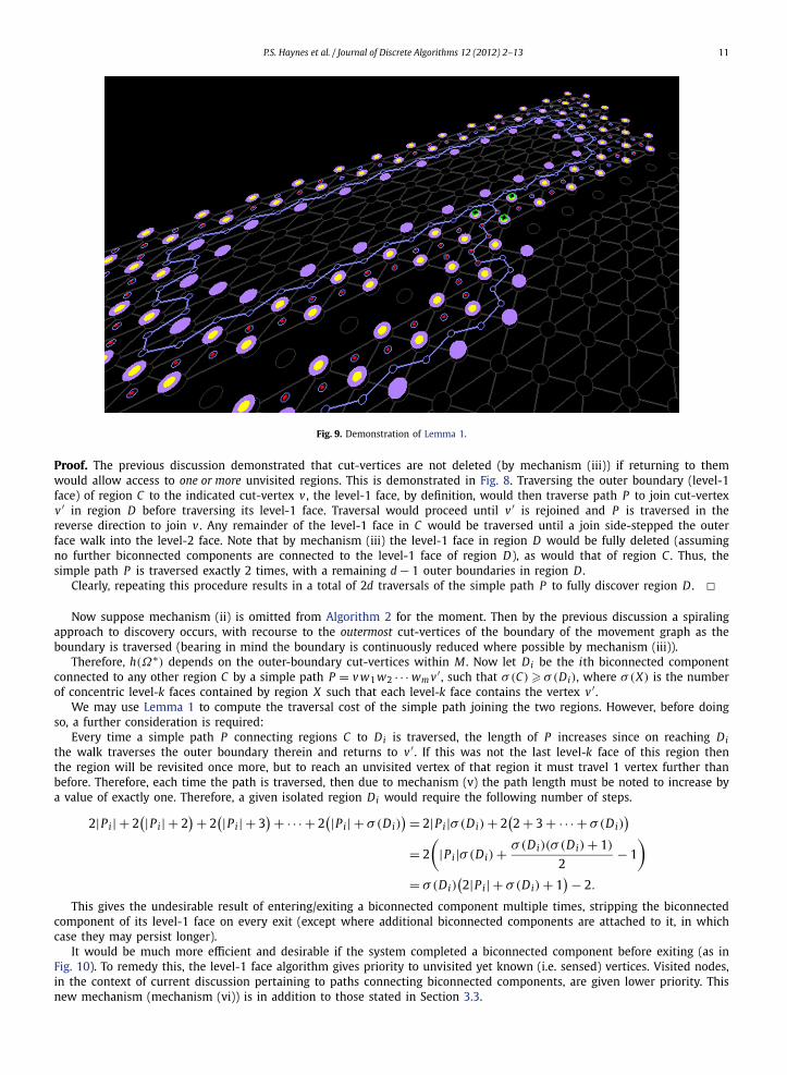
An inefficient property of the mechanisms presented so far concerns the existence of biconnected components con-nected by a path, however short, one or more of which may contain a number of concentric level-k faces (see Fig. 8). Thisinefficiency is highlighted by the following lemma.

Fig. 8. Concentric level-k faces of two regions C and D of graph G connected by a simple path P = v w1 w2 · · · wm v ′ .

Lemma 1. Let biconnected components C and D be two regions of M∗ , connected by a simple path P = v w1 w2 · · · wm v ′ , containingquantities c and d of level-k faces respectively such that c � d. Then P must be traversed 2d times to discover D fully.


Fig. 9. Demonstration of Lemma 1.

Proof. The previous discussion demonstrated that cut-vertices are not deleted (by mechanism (iii)) if returning to themwould allow access to one or more unvisited regions. This is demonstrated in Fig. 8. Traversing the outer boundary (level-1face) of region C to the indicated cut-vertex v , the level-1 face, by definition, would then traverse path P to join cut-vertexv ′ in region D before traversing its level-1 face. Traversal would proceed until v ′ is rejoined and P is traversed in thereverse direction to join v . Any remainder of the level-1 face in C would be traversed until a join side-stepped the outerface walk into the level-2 face. Note that by mechanism (iii) the level-1 face in region D would be fully deleted (assumingno further biconnected components are connected to the level-1 face of region D), as would that of region C . Thus, thesimple path P is traversed exactly 2 times, with a remaining d − 1 outer boundaries in region D .

Clearly, repeating this procedure results in a total of 2d traversals of the simple path P to fully discover region D . �Now suppose mechanism (ii) is omitted from Algorithm 2 for the moment. Then by the previous discussion a spiraling

approach to discovery occurs, with recourse to the outermost cut-vertices of the boundary of the movement graph as theboundary is traversed (bearing in mind the boundary is continuously reduced where possible by mechanism (iii)).

Therefore, h(Ω∗) depends on the outer-boundary cut-vertices within M . Now let Di be the ith biconnected componentconnected to any other region C by a simple path P = v w1 w2 · · · wm v ′ , such that σ(C) � σ(Di), where σ(X) is the numberof concentric level-k faces contained by region X such that each level-k face contains the vertex v ′ .

We may use Lemma 1 to compute the traversal cost of the simple path joining the two regions. However, before doingso, a further consideration is required:

Every time a simple path P connecting regions C to Di is traversed, the length of P increases since on reaching Dithe walk traverses the outer boundary therein and returns to v ′ . If this was not the last level-k face of this region thenthe region will be revisited once more, but to reach an unvisited vertex of that region it must travel 1 vertex further thanbefore. Therefore, each time the path is traversed, then due to mechanism (v) the path length must be noted to increase bya value of exactly one. Therefore, a given isolated region Di would require the following number of steps.

2|Pi| + 2(|Pi| + 2

) + 2(|Pi | + 3

) + · · · + 2(|Pi| + σ(Di)

) = 2|Pi |σ(Di) + 2(2 + 3 + · · · + σ(Di)

)

= 2

(|Pi|σ(Di) + σ(Di)(σ (Di) + 1)

2− 1

)

= σ(Di)(2|Pi| + σ(Di) + 1

) − 2.

This gives the undesirable result of entering/exiting a biconnected component multiple times, stripping the biconnectedcomponent of its level-1 face on every exit (except where additional biconnected components are attached to it, in whichcase they may persist longer).

It would be much more efficient and desirable if the system completed a biconnected component before exiting (as inFig. 10). To remedy this, the level-1 face algorithm gives priority to unvisited yet known (i.e. sensed) vertices. Visited nodes,in the context of current discussion pertaining to paths connecting biconnected components, are given lower priority. Thisnew mechanism (mechanism (vi)) is in addition to those stated in Section 3.3.


Fig. 10. The walk completes isolated regions, unlike in Fig. 8.

Thus, in Fig. 9 the biconnected component shown would cause Algorithm 1 to consider the cut-vertex dual to the 3-clique as inaccessible. This has the effect of the next level-1 face computed to be that of the interior of the biconnectedcomponent. This process continues until the biconnected component is fully explored at which point the region is exited.

This simple addition gives a much improved performance, and will in fact seek out the furthest possible biconnectedcomponents, completing biconnected components from the furthest reaches backwards to the starting point. This includesnested biconnected components, meaning that very complex environments are efficiently discovered.

Given the previous discussion and the introduction of mechanism (vi), we can deduce an estimate for a maximum boundof h(Ω∗),

h(Ω∗) �

∣∣M∗∣∣ + 2p−1∑k=1

|Pk|,

where p is the number of biconnected components emerging as M develops and Pk are paths connecting their centres.

4.3. Overall complexity

Consider the final movement graph M∗ . We know there exists an induced subgraph Ω ∈ M∗ , where Ω is the final pathtaken, such that the 3-clique of robots traverse M∗ as optimal as the rules governing Algorithm 2 allow. The upper boundof exactly how optimal was given above. Thus, since |Ω| � |M∗| = nH , we are justified in basing all deductions concerningcomplexity of the algorithm to search an unknown environment on the input size nH .

We know that Algorithm 2 is called nH times. Looking at Algorithm 2, the very nature of when (if at all) and for whatconstant of complexity some of the internal functions of Algorithm 2 are called depends on the environment. Thus, we maydeduce that the algorithm to search an entire unknown environment takes O (k · nH ), where 1 � k < nH is to be determinedand depends entirely on the environment. The trivial example of a square environment, with no internal features, forexample, would correspond to k = 1. This is also true for many graphs with internal features. By definition of Algorithm 2,k is always less than nH since the initial movement graph is an induced subgraph of M. Thus, the internal algorithms ofAlgorithm 2 do not operate on all nH nodes initially, if at all ever. We are currently investigating an upper bound for k.

5. Closing remarks

This paper gives a solution to the difficult problem of unknown environment search using graph structures and elementsof graph theory.

On imposing a virtual structure on the environment, a principle of search, basically amounting to wall following, wasdeveloped into a number of algorithms and additional mechanisms were reasoned and applied to achieve a desired resulteach of which improved efficiency of the search in some way.

The result is a simple, discrete, and robust system of O (k · nH ) complexity which is both useful in its current form yetallowing room for further development.

The authors believe this to be a novel approach in that the system assigns virtual structure to the environment thus avail-ing pragmatic deployment of entities within the environment and eventual metric map construction. Previous approachestraditionally overlay the topological structure once the environment has been searched and a metric map built.

Future work will include improvement (possibly by way of convolution) of algorithms, and theoretical improvements ofthe walk length upper bound. Walk length could be improved by changing from spiral wall following, which completesdiscovery of a biconnected component at the centre of the component, to an alternating sweep of the outer most wall ofthe component. This would complete discovery of the biconnected component with the 3-clique at the position where itfirst entered the component, thus reducing the maximum bound on the walk length. Investigation of the classification ofdifferent environment graphs and their effects on the value of k in the overall complexity of the algorithm would also be ofinterest.


Practical applications on a real world problem (such as robots) is a major goal, and recent work has shown that the outerface walk (Algorithm 1) can be optimized to consider only local graph vertices (much like Algorithm 4 does), thus reducingit to constant time complexity.

Finally, development of algorithms to coordinate n entities for efficient search is desirable, for large team exploration, forexample.

References

[1] L.S. Alboul, H. Abdul-Rahman, P.S. Haynes, J. Penders, An approach to multi-robot site exploration based on principles of self-organization, in: Intelli-gent Robotics and Applications – Third International Conference, ICIRA 2010, Proceedings, Part II, Shanghai, China, November 10–12, 2010, in: LNCS,vol. 6425, Springer, 2010, pp. 717–729.

[2] L. Alboul, G. Echeveria, M. Rodrigues, Curvature criteria to fit curves to discrete data, in: EWCG 19th European Workshop on Computational Geometry,2004.

[3] T. Bailey, H. Durrant-Whyte, Simultaneous localisation and mapping (SLAM): part II, IEEE Robotics and Automation Magazine 13 (3) 108-117.[4] B.S. Baker, Approximation algorithms for NP-complete problems on planar graphs, Journal of the Association for Computing Machinery 41 (1) (1994)

153–180.[5] Dieter Fox, Wolfram Burgard, Hannes Kruppa, Sebastian Thrun, A probabilistic approach to collaborative multi-robot localisation, Autonomous

Robots 8 (3) (2000) 325–344.[6] D. Fox, J. Ko, K. Konolige, B. Limketkai, D. Schulz, B. Stewart, Distributed Multirobot exploration and mapping, Proceedings IEEE 94 (7) (2006) 1325–

1339.[7] B. Gerkey, M. Mataric, Multi-robot task allocation: Analyzing the complexity and optimality of key architectures, in: Proc. of the IEEE International

Conference on Robotics and Automation (ICRA), 2003.[8] A. Howard, M.J. Mataric, G.S. Sukhatme, Localisation for mobile robot teams: A distributed MLE approach, in: Experimental Robotics, in: Advanced

Robotics Series, vol. VIII, 2002, pp. 146–166.[9] K.R. Kurazume, S. Hirose, An experimental study of a cooperative positioning system, Autonomous Robots 8 (1) (2000) 4352.

[10] L. Ludwig, M. Gini, Robotic swarm dispersion using wireless intensity signals, in: Distributed Autonomous Robotic Systems, vol. 7, Springer, Japan,2007, pp. 135–144.

[11] M. Mesbahi, M. Egerstedt, Graph Theoretical Methods in Multiagent Networks, Princeton University Press, 2010.[12] I. Rekleitis, G. Dudek, E. Milios, Multi-robot collaboration for robust exploration, Annals of Mathematics and Artificial Intelligence 31 (2001) 7–40.[13] K. Takamizawa, T. Nishizeki, N. Saito, An algorithm for finding a short closed spanning walk in a graph, Networks 10 (1980) 249–263.[14] W.T. Tutte, A theorem on planar graphs, Transactions of American Mathematical Society 82 (1956) 99–116.[15] W.T. Tutte, Bridges and Hamiltonian circuits in planar graphs, Aequationes Mathematica 15 (1977) 1–33.[16] N. Vlassis, G. Papakonstantinou, P. Tsanakas, Robot map building by Kohonen’s self-organizing neural networks, in: Proc. 1st Mobinet Symposium on

Robotics for Health, 1997.

Documents

Dynamic graph-based search in unknown environments