Embed Size (px)
Citation preview
Int. J. Mechatronics and Automation, Vol. 4, No. 3, 2014 173
Copyright © 2014 Inderscience Enterprises Ltd.
Cooperative navigation of unknown environments using potential games
George Philip* Department of Systems and Computer Engineering, Carleton University, Ottawa, Ontario, Canada E-mail: [email protected] *Corresponding author
Sidney N. Givigi Jr. Department of Electrical and Computer Engineering, Royal Military College of Canada, Kingston, Ontario, Canada E-mail: [email protected]
Howard M. Schwartz Department of Systems and Computer Engineering, Carleton University, Ottawa, Ontario, Canada E-mail: [email protected]
Abstract: In this paper, we develop a method of exploring a 2-D environment with multiple robots by modelling the problem as a potential game rather than using conventional frontier-based dynamic programming algorithms. A potential game is a type of game that results in coordinated behaviours amongst players. This is done by enforcing strict rules for each player in selecting an action from its action set. As part of this game, we define a potential function for the game that is meaningful in terms of achieving the greater objective of exploring a space. Furthermore, an objective function is assigned for each player from this potential function. We then create an algorithm for the exploration of an obstacle-filled bounded space, and demonstrate through simulation how it outperforms an uncoordinated algorithm by reducing the time needed to uncover the space. Analysis of the computational complexity of the algorithm will show that the algorithm is of O(sRange2), where sRange is the range of a sensor on a robot. We then suggest an improvement to the proposed algorithm that is premised on having a robot predict the future positions of all other robots.
Keywords: weakly acyclic game; potential game; robotics; simultaneous localisation and mapping problem; SLAM; game theory; exploration.
Reference to this paper should be made as follows: Philip, G., Givigi Jr., S.N. and Schwartz, H.M. (2014) ‘Cooperative navigation of unknown environments using potential games’, Int. J. Mechatronics and Automation, Vol. 4, No. 3, pp.173–187.
Biographical notes: George Philip received his BASc in Electrical Engineering from the University of Waterloo, and MASc in Systems and Computer Engineering from Carleton University. His research interests include adaptive control systems, machine learning, and game theory in robotics.
Sidney N. Givigi Jr. is an Assistant Professor in the Electrical and Computer Engineering Department at the Royal Military College of Canada. His expertise is in robotics and control systems. In particular, his research interests include real-time systems, non-linear and chaotic systems, and game theory.
Howard M. Schwartz is a Professor in the Systems and Computer Engineering Department at Carleton University. His research interests include adaptive and intelligent control systems, robotics, system modelling and system identification. His most recent research is in multi agent learning with applications to teams of mobile robots.

174 G. Philip et al.
This paper is a revised and expanded version of a paper entitled ‘Multi-robot exploration using potential games’ presented at IEEE International Conference on Mechatronics and Automation, Takamatsu, Japan, August 4–7, 2013.
1 Introduction
The field of robotics has seen much development and research in recent years. The problem of exploring an unknown environment and generating a map for it remains an active area for research and is at the heart of mobile robotics. Applications for this problem can be found in planetary exploration, reconnaissance, rescue, etc., in which complete coverage of a terrain is important (Burgard et al., 2000). Recently, these applications have been extended to include underwater systems in accomplishing various tasks using autonomous underwater vehicles (AUVs). This includes mapping of mines underwater and the mapping of the topography under polar ice caps (Wadhams, 2012). Furthermore, applications involving the use of multiple robots in achieving cooperative tasks have received a considerable amount of attention. A multi-agent system consists of a number of intelligent agents that interact with other agents in a multi-agent environment. An agent is an autonomous entity that observes the environment and takes an action to satisfy its objective based on its knowledge (Lu, 2012). The major challenge in multiagent systems arise from the fact that agents have limited knowledge about the status of other agents, except perhaps for a small subset of neighbouring agents. Agents are endowed with a utility function or reward that depends on their own strategies and the strategies of other agents. As such, in situations where agents know nothing about the structure of their utility functions or how their own utility depends on the actions of other agents, the only course of action for them is to observe rewards based on experience and ‘optimise’ on a trial and error basis (Marden et al., 2009a). Also, as all agents are trying simultaneously to optimise their own strategies, even in the absence of noise, an agent trying the same strategy twice may see different results because of the non-stationary nature of the strategies of other agents. The situation is only further complicated when the environment is dynamic as in Sun et al. (2012), where robots intelligently re-plan new routes as the environment changes.
The exploration and the mapping of an environment is a challenge in that the environment is completely unknown and there is no pre-existing map for a robot to localise itself within. Having multiple robots explore and map out the space adds to the complexity because as with any multi-agent system the environment becomes dynamic and complex (Lu, 2012). Not only do robots have to simultaneously explore the environment while avoiding obstacles and barriers and locate these features on a map, but they also have to coordinate themselves so that their numbers can be used to efficiently navigate the space. In addition, since each robot does not follow the same path or
trajectory to explore the space, they have a different view of the environment. These different views of the environment have to be merged together to create a unified view or map of the environment. Robots that simultaneously explore an environment to map it while localising itself within that environment is solving what is known as the simultaneous localisation and mapping problem (SLAM) or the concurrent mapping and localisation (CML) problem (Castellanos et al., 2001; Dissanayake et al., 2000). There is extensive literature on SLAM, which focus on different aspects of SLAM from robot dynamics, environment dynamics (e.g., indoor, outdoor, moving or static objects), and the framework for combining sensor information (e.g., extended Kalman filter, particle filter) to more recently utilising different sensors such as cameras rather than lasers as seen in Asmar and Shaker (2012). Furthermore, methods have been proposed to address changing degrees of environmental complexity in real-time SLAM applications, which require different models to estimate the modes of behaviour. This is done in Wong et al. (2013) by having an integrated schema which mixes the interactive multiple model (IMM) and joint probabilistic data association (JPDA), with the asymmetric assignment optimisation algorithm.
In this paper, we look at using multiple robots for the purpose of navigating and exploring a bounded 2-D space that consists of obstacles. We are more interested in the navigation algorithms employed by robots to fully explore a space than the mapping aspect. As such, we assume that robots are able to localise themselves within a bounded region. Specifically, this paper looks at the application of potential games in having multiple robots collaboratively explore a space rather than using conventional Frontier-detection algorithms.
1.1 Background
The goal of exploration is to gain as much new information as possible of the environment within bounded time (Keidar and Kaminka, 2012). In most applications today that involve the use of multiple robots to explore a space, a variation of the Frontier-based dynamic programming (DP) algorithm introduced in Burgard et al. (2000) is utilised. This approach involves choosing appropriate target points for the individual robots so that they simultaneously explore different regions of the environment. Coordination is achieved by simultaneously taking into account the cost of reaching a target point and its utility (Burgard et al., 2000). Whenever a target point is assigned to a specific robot, the utility of the unexplored area visible from this target position is reduced for the other robots. In this way,
Cooperative navigation of unknown environments using potential games 175
different target locations are assigned to individual robots (Burgard et al., 2000). Using this approach every robot is required to keep track of the Frontier cells, which is the boundary between unexplored and explored cells. To determine the cost of reaching the current Frontier cells, the optimal path from the current position of the robot to all Frontier cells is computed based on a deterministic variant of value iteration, a popular DP algorithm (Bellman, 1957; Howard, 1960). Thus, the cost of reaching each cell in the explored space must be calculated. As it can take several iterations to converge to a final cost value for each cell, the computational complexity grows as the robots explore more space. In fact, the computational complexity is of quadratic order of the size of the explored area. The second issue with this approach is that much information has to be shared among robots to achieve coordination. Among other variables that must be shared, each robot has to share with other robots its cost of reaching the Frontier cell that is closest to it. Furthermore, as part of the coordination scheme each player has to consider the decision the other players would take at a given time and the respective payoffs they would receive before the player can evaluate its own payoff for a particular action choice. Thus, considering the aforementioned facts about Frontier-based DP algorithms, it would be of interest to investigate a method that may reduce computational complexity for large search spaces; have a robot determine the action it should take without having to calculate the decision of other robots; and that reduces the information that needs to be shared among robots. It is generally known that game theory offers advantages in that it leads to decentralised systems and reduces computational complexity (Lindsay, 2011). In this regard, we come up with a method of exploring a space using multiple robots by modelling the problem as a potential game.
Section 2.1 will introduce a well established class of non-cooperative games known as the weakly acyclic game, which a potential game is a subclass of. It will also introduce the simple forward turn controller from Lindsay (2011), which is a mechanism for accounting the lateral motion experienced by a robot when it performs a turn in a non-holonomic environment. We will integrate the simple forward turn controller in our solution for exploring a space using multiple robots. Section 2.2 will identify a shortcoming of weakly acyclic games and briefly discuss how potential games addresses this problem. In Section 2.3, the potential game itself will be defined. Furthermore, the potential function of our game will be defined in terms of the goal we are trying to achieve, and from this, the objective function of a player will be assigned. In Section 2.4, an algorithm will be derived based on our game, which will then be modified in Section 3 so that bounded spaces with obstacles can be explored by robots. The resulting algorithm’s computational complexity will be analysed in Section 3.1, and finally an improved algorithm that is based on predicting the future locations of robots will be discussed in Section 4.
1.2 Contributions
The main contributions of this paper are:
1 The collaborative mapping of an unknown environment with a team of robots using potential games. As part of this contribution, we extend the definition of a potential game so that it can be modelled under the framework of the simple forward turn controller.
2 We define a potential function and objective function for our potential game that is meaningful in terms of achieving the greater objective of exploring a space. Moreover, update rules for crucial variables in the potential game will be presented, and a proof of our game satisfying a potential game will be presented.
3 The derivation of an algorithm from our potential game that allows a finite bounded space to be explored by multiple robots.
4 The complexity analysis of our potential game algorithm, which will be found to have a lower runtime order than Frontier detection algorithms.
5 The improvement of our initial potential game algorithm. The improvement stems from having a robot predict the future location of every other robot when it decides to turn. New update rules will also be presented for key variables as part of this new algorithm.
2 Weakly acyclic and potential games
2.1 Weakly acyclic games
Weakly acyclic games are a class of games that unlike what is often encountered in cooperative robotics, provides robust group behaviours for robots while only placing gentle restrictions on the robots’ selection of actions (Lindsay, 2011). “Informally, a weakly acyclic game is one where natural distributed dynamics, such as better-response dynamics, cannot enter inescapable oscillations” (Fabrikant et al., 2010). This definition implies that players can start with any action and so long as there exists a pure Nash equilibrium, the players will reach it by changing their actions throughout the course of the game, which will result in a corresponding increase in their utility. The following definitions have to be established to formalise a weakly acyclic game.
Definition 2.1 (better-response actions): An action i ia A′ ∈ is a better-response of player i to an action profile (ai, a–i) if
( ) ( )i i i i i iU a a U a a− −′ − > − (Fabrikant et al., 2010), where a−i refers to the joint actions of all the players except i and ui refers to the utility or objective function of player i.
176 G. Philip et al.
Definition 2.2 (better response path): A better response path in a game G is a sequence of action profiles a1, ..., ak in that for every j ∈ [1, ..., k − 1] two conditions are met:
1 aj and aj+1 only differ in the action of a single player i
2 player i at time step j + 1 is a better response action, i.e., 1( , ) ( , )j j j j
i i i i i iU a a U a a+− −> (Lindsay (2011;
Fabrikant et al., 2010).
The second part of Definition 2.2 implies that the utility received by the player changing its action at a given time must be greater than the utility it would receive if it did not change its action.
Definition 2.3 (weakly acyclic games): A game G is weakly acyclic if for any action profile a ∈ A, there exists a better response path starting at action a, and ending at some pure Nash equilibrium of G (Lindsay, 2011; Fabrikant et al., 2010), where A represents the set of all joint action vectors for all the players in the game.
A limiting factor in a weakly acyclic game lies in the first part of Definition 2.2, which requires that only one player changes its action at every time step. Thus if a strict weakly acyclic game is used as a solution to solve a cooperative robotics problem it would require that a centralised entity determine which player will change its action at every time step. This is, however, very undesirable because it would make it a centralised system. Another option is to let the players change their actions at a random specified rate, ε, which is known as the exploration rate (Marden et al., 2009a). It was found in Marden et al. (2009a) that using the exploration rate option, it is never guaranteed that a Nash equilibrium will be found, but if ε is small and if the time step t is significantly large, the Nash equilibrium will be found with a high probability. This theory was incorporated in Lindsay (2011) knowing that there is a slight probability that for a small number of tests, a Nash equilibrium consensus point would not be reached.
The consensus problem, which is the problem of getting a group of autonomous robots to meet at a point without having a centralised algorithm telling the robots where that point is Lindsay (2011), was solved in Marden et al. (2009a) and Blume (1996). Although Marden et al. (2009a) and Blume (1996) guaranteed results to the consensus problem when it is modelled as a weakly acyclic game, it did not allow for non-holonomic behaviour. Thus the algorithms could not be implemented as controllers on actual robots that may for example use a differential drive system. In Lindsay (2011), a mechanism known as a simple forward turn controller was devised as part of a weakly acyclic game to solve the consensus problem in a non-holonomic environment. The lateral motion experienced by a robot when it turns is accounted for in the simple forward turn controller by having the robot change its pose or orientation in one time step, and then having it move forward with the new pose in the following time step for one time step. Thus, when a robot turns it does so over two time steps over a sequence of two different actions (a ‘turn action’ and a
‘move forward’ action). We call this a two-step action sequence. This restriction in having to perform a turn over two times steps is how the non-holonomic behaviour of a robot is modelled. The idea of having a two-step action sequence is that it would impact the utility the robot would receive over the course of the turn sequence in comparison to the utility it would get if a whole turn (which includes a robot’s lateral movement and its movement forward) was executed in one time step. This will be seen in Section 2.3. We will utilise the simple forward turn controller in our algorithm.
The following subsections discuss the workings of the simple forward turn controller as seen in Lindsay (2011), which includes initialisation and the action-selection policy based on the expected utilities. However, we first need to establish an action set for each of the robots in a similar manner as Lindsay (2011). We will arbitrarily assign each robot in our game an action set, Ai, that has without loss of generality four actions. This is sufficient for any robot to get to any point in a 2-D environment.
{ }1 2 3 4, , , ,i i i i iA a a a a= (1)
where 1ia is the action ‘move forward’, 2
ia ‘turn 90°’, 3ia
‘turn 180°’, 4ia ‘turn −90°’.
2.1.1 Initialisation
At the first time step, t = 0, each player will randomly select a pose. In the next time step each of the robots will execute
1ia (‘move forward’). The combination of the ‘move
forward’ command and the pose of a robot constitutes what is known as its baseline action b
ia (Lindsay, 2011).
2.1.2 Action selection
At each time step, each robot is given a choice to play its baseline action by moving forward with a probability of (1 − ε) or to explore by performing a turn sequence with a probability ε.
2.1.3 Baseline action and turn sequence
When player i plays the baseline action and does not explore, it moves in the direction that the baseline action specifies. We denote a two-step action sequence of a player i as 1( , ) ,x
i i ia a α∈ where xi ia A∈ in (1), and the sequence of
actions is xia followed by 1,ia the ‘move forward’
command. There are four two-step actions sequences that are possible for the action set specified in (1). They are
( ) ( ) ( ) ( ){ }1 1 2 1 3 1 4 1, , , , , , ,i i i i i i i i ia a a a a a a aα = (2)
Notice here that 1xi ia a= represents the baseline action.
Figure 1 shows a robot i’s predicted positions in a grid game for playing each two-step action sequence in αi. The arrow
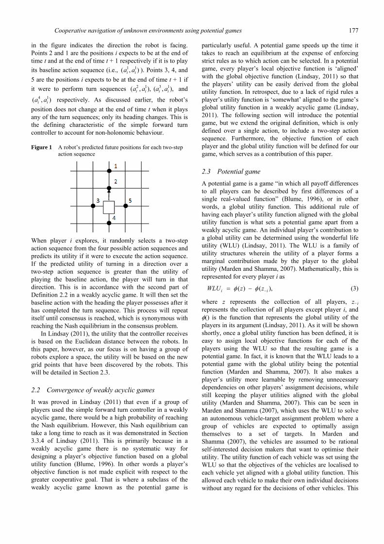
Cooperative navigation of unknown environments using potential games 177
in the figure indicates the direction the robot is facing. Points 2 and 1 are the positions i expects to be at the end of time t and at the end of time t + 1 respectively if it is to play its baseline action sequence (i.e., 1 1( , )i ia a ). Points 3, 4, and 5 are the positions i expects to be at the end of time t + 1 if it were to perform turn sequences 2 1 3 1( , ), ( , ),i i i ia a a a and
4 1( , )i ia a respectively. As discussed earlier, the robot’s position does not change at the end of time t when it plays any of the turn sequences; only its heading changes. This is the defining characteristic of the simple forward turn controller to account for non-holonomic behaviour.
Figure 1 A robot’s predicted future positions for each two-step action sequence
When player i explores, it randomly selects a two-step action sequence from the four possible action sequences and predicts its utility if it were to execute the action sequence. If the predicted utility of turning in a direction over a two-step action sequence is greater than the utility of playing the baseline action, the player will turn in that direction. This is in accordance with the second part of Definition 2.2 in a weakly acyclic game. It will then set the baseline action with the heading the player possesses after it has completed the turn sequence. This process will repeat itself until consensus is reached, which is synonymous with reaching the Nash equilibrium in the consensus problem.
In Lindsay (2011), the utility that the controller receives is based on the Euclidean distance between the robots. In this paper, however, as our focus is on having a group of robots explore a space, the utility will be based on the new grid points that have been discovered by the robots. This will be detailed in Section 2.3.
2.2 Convergence of weakly acyclic games
It was proved in Lindsay (2011) that even if a group of players used the simple forward turn controller in a weakly acyclic game, there would be a high probability of reaching the Nash equilibrium. However, this Nash equilibrium can take a long time to reach as it was demonstrated in Section 3.3.4 of Lindsay (2011). This is primarily because in a weakly acyclic game there is no systematic way for designing a player’s objective function based on a global utility function (Blume, 1996). In other words a player’s objective function is not made explicit with respect to the greater cooperative goal. That is where a subclass of the weakly acyclic game known as the potential game is
particularly useful. A potential game speeds up the time it takes to reach an equilibrium at the expense of enforcing strict rules as to which action can be selected. In a potential game, every player’s local objective function is ‘aligned’ with the global objective function (Lindsay, 2011) so that the players’ utility can be easily derived from the global utility function. In retrospect, due to a lack of rigid rules a player’s utility function is ‘somewhat’ aligned to the game’s global utility function in a weakly acyclic game (Lindsay, 2011). The following section will introduce the potential game, but we extend the original definition, which is only defined over a single action, to include a two-step action sequence. Furthermore, the objective function of each player and the global utility function will be defined for our game, which serves as a contribution of this paper.
2.3 Potential game
A potential game is a game “in which all payoff differences to all players can be described by first differences of a single real-valued function” (Blume, 1996), or in other words, a global utility function. This additional rule of having each player’s utility function aligned with the global utility function is what sets a potential game apart from a weakly acyclic game. An individual player’s contribution to a global utility can be determined using the wonderful life utility (WLU) (Lindsay, 2011). The WLU is a family of utility structures wherein the utility of a player forms a marginal contribution made by the player to the global utility (Marden and Shamma, 2007). Mathematically, this is represented for every player i as
( ) ( ),i iWLU z zφ φ −= − (3)
where z represents the collection of all players, z−i represents the collection of all players except player i, and φ() is the function that represents the global utility of the players in its argument (Lindsay, 2011). As it will be shown shortly, once a global utility function has been defined, it is easy to assign local objective functions for each of the players using the WLU so that the resulting game is a potential game. In fact, it is known that the WLU leads to a potential game with the global utility being the potential function (Marden and Shamma, 2007). It also makes a player’s utility more learnable by removing unnecessary dependencies on other players’ assignment decisions, while still keeping the player utilities aligned with the global utility (Marden and Shamma, 2007). This can be seen in Marden and Shamma (2007), which uses the WLU to solve an autonomous vehicle-target assignment problem where a group of vehicles are expected to optimally assign themselves to a set of targets. In Marden and Shamma (2007), the vehicles are assumed to be rational self-interested decision makers that want to optimise their utility. The utility function of each vehicle was set using the WLU so that the objectives of the vehicles are localised to each vehicle yet aligned with a global utility function. This allowed each vehicle to make their own individual decisions without any regard for the decisions of other vehicles. This
178 G. Philip et al.
aspect of the WLU that allows an agent to make decisions without considering other’s decisions is highly beneficial over other methods such as reinforcement learning techniques and Frontier-based DP methods, which require each agent to know the actions taken by other agents.
Before we set up our potential game, we need to create a grid where the game will be played. The grid represents the space which the robots will explore. If we divide the space equally so that there is Z horizontal divisions and Z vertical divisions, we will have a Z × Z grid. A grid point is the intersection of a horizontal line and a vertical line. They serve as reference points in calculating utilities as it will be seen shortly. Furthermore, as before the group of players or robots in the potential game is represented by N = {1, 2, 3, ..., n} where n is the number of players. In this setting, each player i ∈ N is assigned a two-step action sequence set αi and a local objective function 1(( , ),( )) : x
i i i i iU a a a a α− −′ ′′− →Z
where ii Nα α
∈=∏ is the set of joint two-step action
sequences. Before we define the function 1(( , ),( )),xi i i i iU a a a a− −′ ′′−
however, we first define an intermediary objective function for a player for a single time step as opposed to two time steps in a two-step action sequence to make the definition easier to follow. In a similar manner as Lindsay (2011) we assign a player i’s objective function for a single time step at a time t for a given action .x
i ia A∈ . Note that t is an instance of time in the discrete time domain.
( ) [ ]( ) ( 1), ,xia
i i ipt gridpts
U pos t f pos t pt∈
= +∑ (4)
where
[ ]1, if ( )
( 1), 1, if 1 or 2 is true0, otherwise
i
i
pt discPts tf pos t pt C C
∈⎧⎪+ = ⎨⎪⎩
C1 evaluates to true if
( ) and ( ),i ipt loc t sRange pt discP ts t−− ≤ ∉
C2 evaluates to true if
( 1) and ( ),i ipt loc t sRange pt discP ts t−− + ≤ ∉
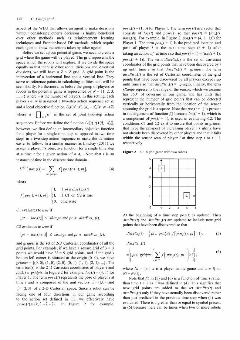
and gridpts is the set of 2-D Cartesian coordinates of all the grid points. For example, if we have a square grid of 3 × 3 points we would have 32 = 9 grid points, and if the grid’s bottom-left corner is situated at the origin (0, 0), we have gridpts = {(0, 0), (1, 0), (2, 0), (0, 1), (1, 1), (2, 1), ...}. The term loci(t) is the 2-D Cartesian coordinates of player i and loci(t) ∈ gridpts. In Figure 2 for example, loci(t) = (4, 1) for Player 1. The term posei(t) represents the pose of player i at time t and is composed of the unit vectors ˆ {1,0}x = and ˆ {1,0}y = of a 2-D Cartesian space. Since a robot can be
facing one of four directions in our game according to the action set defined in (1), we effectively have
ˆ ˆ ˆ ˆ( ) { , , , }.ipose t x y x y∈ − − In Figure 2 for example,
posei(t) = (1, 0) for Player 1. The term posi(t) is a vector that consists of loci(t) and posei(t) so that posi(t) = (loci(t), posei(t)). For example, in Figure 2, posi(t) = (4, 1, 1,0) for Player 1. The term posi(t + 1) is the predicted location and pose of player i at the next time step (t + 1) after taking an action x
ia at time t so that posi(t + 1) = (loci(t + 1), posei(t + 1)). The term discPtsi(t) is the set of Cartesian coordinates of the grid points that have been discovered by i up until time t so that discPtsi(t) ⋇ gridpts. The term discPts−i(t) is the set of Cartesian coordinates of the grid points that have been discovered by all players except i up until time t so that discPts−i(t) ⋇ gridpts. Finally, the term sRange represents the range of the sensor, which we assume has 360° of coverage in our game, and has units that represent the number of grid points that can be detected vertically or horizontally from the location of the sensor assuming the grid is a square. Note that posi(t + 1) is present in the argument of function f() because loci(t + 1), which is a component of posi(t + 1), is used in evaluating C2. The conditions C1 and C2 exist to ensure that points in gridpts that have the prospect of increasing player i’s utility have not already been discovered by other players and that it falls within the sensor scan of player i at time step t or t + 1 respectively.
Figure 2 6 × 6 grid game with two robots
At the beginning of a time step posi(t) is updated. Then discPtsi(t) and discPts−i(t) are updated to include new grid points that have been discovered so that
[ ]{ }( ) ( ), 1 ,i idiscPts t pt gridpts f pos t pt= ∈ = (5)
( )
( ), 1 ,i
i
jj N
discPts t
pt gridpts f pos t pt
−
∈
⎧ ⎫⎛ ⎞⎪ ⎪⎜ ⎟⎡ ⎤= ∈ ≥⎨ ⎬⎣ ⎦⎜ ⎟⎪ ⎪⎝ ⎠⎩ ⎭∑ (6)
where Ni = {x | x is a player in the game and x ≠ i} or Ni = N\{i}.
Note that f() in (5) and (6) is a function of time t rather than time t + 1 as it was defined in (4). This signifies that new grid points are added to the set discPtsi(t) and discPts−i(t) only if they have actually been discovered rather than just predicted in the previous time step when (4) was evaluated. There is a greater than or equal to symbol present in (6) because there can be times when two or more robots

Cooperative navigation of unknown environments using potential games 179
have overlapping sensor coverage, which can lead to a grid point being discovered by more than one robot. More will be said about this in Section 2.4. Finally, the predicted utility for each two-step action sequence 1( , )x
i ia a is calculated. This is done as opposed to just predicting the utility of one action because if we assume a player has a 360° view or sensor coverage, the turn action alone at time t will not change its utility at time t + 1. This is because the robot will remain in the exact same position at the end of the time step t as seen in Figure 1. It has to move forward at time t + 1 if its predicted utility is to increase. This can be seen in the definition of the objective function of a player in (4), where only the discovery of new grid points at a time t + 1 causes the objective function ( ( ))
xia
i iU pos t to change
from ( ( 1)).xia
i iU pos t − Hence, we now define the objective function for a player i for a two-step action sequence based on its objective function for a single time step. Ui
( ) ( )( )
[ ]
1
1, ,
( ( 1))
( 2), ,
i
xi i i i i
ai i
ipt gridpts
U a a a a
U pos t
f pos t pt
− −
∈
′ ′′−
= +
= +∑ (7)
where as previously mentioned 1(( , ), ( )) : x
i i i i iU a a a a α− −′ ′′− → Z and .ii Nα α
∈=∏ Based
on the definition of f[posi(t + 1), pt] in (4), we evaluate f[posi(t + 2), pt] to be the following.
[ ]1, if ( 1)
( 2), 1, if 1 or 2 is true0, otherwise
i
i
pt discPts tf pos t pt C C
∈ +⎧⎪+ = ⎨⎪⎩
C1 evaluates to true if
( 1) and ( 1),i ipt loc t sRange pt discP ts t−− + ≤ ∉ +
C2 evaluates to true if
( 2) and ( 1),i ipt loc t sRange pt discPts t−− + ≤ ∉ +
The left-hand side of (7) represents the predicted utility of a two-step action sequence 1( , )x
i i ia a α∈ for a player i at time t amidst the sequence of actions taken by the other players during the two-step action sequence, denoted here by ( ).i ia a− −′ ′′− In the right-hand side of the equation, posi(t + 1) represents the position and pose of player i after it has executed the first action x
ia in the two-step action sequence 1( , ).x
i ia a Therefore, the right-hand side of the equation represents player i’s predicted utility at the end of the second time step t + 1 after it has executed the second action of the two-step action sequence, which by the definition of a player’s objective function in (4) is inclusive of the utility it would have had in the previous time step t. Thus, effectively, 1(( , ), ( ))x
i i i i iU a a a a− −′ ′′− is the utility player i predicts to have by the end of the time step t + 1 at time t by
following the two-step action sequence 1( , ).xi ia a We note
two important points here. The first is that player i’s predicted utility of playing the action sequence 1( , )x
i ia a is independent of the sequence of actions ( )i ia a− −′ ′′− played by other players because player i’s objective function as it is defined in (4) is independent of the actions taken by the other players at time t. The position and the pose of the other players are not predicted nor utilised in any way. Secondly, instead of using discPts−i(t + 1) for evaluating the right-hand side of (7) as it would be expected based on (4), discPts−i(t) is used. This is because the prediction is done over two time steps and at time t player i cannot know discPts−i(t + 1). This can only be determined in the next time step after every player has taken an action and has communicated the set of grid points it has discovered to the rest of the players. Thus, it uses the latest knowledge it has, which is discPts−i(t). Another way of stating this is that we assume discPts−i(t + 1) = discPts−i(t). Once the utilities of every two-step action sequence have been predicted, an action is taken based on an action-policy that will be presented in Section 2.4.
We define the potential function of the game as
( )( ) ( ) ,xia
i ii N
t U pos tφ∈
=∑ (8)
Given the potential function in (8), we can see as in Marden et al. (2009b) that with the assignment of the objective function in (4) each player does not have to observe the decision of all players to evaluate its payoff for a particular action choice. This is because if we observe the definition of the potential function and its relation to the objective function of each player in (4), we see that it satisfies the WLU; and as stated in the beginning of this section, the WLU removes unnecessary dependencies of a player’s decisions on other players’ assignment decisions. We define a corresponding potential function φ(γ) : α → Z for (8) that
is a function of the two-step action sequences of all n players rather than time t.
( ) ( )( )1( ) , ,xi i i i i
i N
U a a a aφ γ − −∈
′ ′′= −∑ (9)
where γ ∈ α. By using the WLU formulation in (3), (9) can be written as
( ) ( )( )( ) ( )( )1
1
( ) , ,
, , .
xi i i i i
xj j j j j
i N
U a a a a
U a a a a
φ γ − −
− −∈
′ ′′= −
′ ′′+ −∑ (10)
We now formally define a potential game as it is defined in Marden et al. (2009b), but we extend the definition so that it is for a two-step action sequence rather than a single action.
Definition 2.4 (potential games): Player action sets 1{ } ,ni iα =
together with player objective functions 1{ : } ,ni iU α =→ Z
180 G. Philip et al.
constitute a potential game if, for some potential function φ : α → Z,
( ) ( )( ) ( ) ( )( )( ) ( )( ) ( ) ( )( )
1 1 1 1 1 1
1 1 1 1 1 1
, , , , , ,
, , , , , ,
i i i i i i i i i i
i i i i i i i i
U a a a a U a a a a
a a a a a a a aφ φ
− − − −
− − − −
′ ′′−
′ ′′= − (11)
for every player i ∈ N, for every 1( , ) ,i i ia a α′ ∈ and for every 1( , ) .i i ia a α′′ ∈
Notice in (11) that the second argument of the objective function of player i and the potential function 1 1( , )i ia a− − implying that all players must ‘move forward’ for two time steps or equivalently play their baseline actions while i is playing its two-step action sequence. This is as per the test for a potential game as seen in Marden et al. (2009b), which requires that all players other than player i continue to play their previous action. Since player i is the one changing its action from its baseline action, none of the other players are allowed to change their actions from their respective baseline actions, and thus, must continue to play it. This is also consistent with the first part of Definition 2.2 of a weakly acyclic game (Section 2.1), which a potential game is a subclass of.
Claim 1: Player objective functions (7) constitute a potential game with potential function (9).
Proof: A similar approach as Marden et al. (2009b) will be used to prove the claim. We assume a player i is contemplating at time t whether to turn in one direction by performing the action sequence 1( , )i ia a′ or to turn in another
direction by performing 1( , )i ia a′′ so that .i ia a′ ′′≠ The change in the objective function of player i by switching from the action sequence 1( , )i ia a′′ to the action sequence 1( , ),i ia a′
provided that all other players collectively play 1 1( , ),i ia a− −
( ) ( )( ) ( ) ( )( )1 1 1 1 1 1, , , , , ,i i i i i i i i i i iU U a a a a U a a a a− − − −′ ′′Δ = −
The first difference equation for the potential function of the game for the two different action sequences of player i is
( ) ( )( ) ( ) ( )( )1 1 1 1 1 1, , , , , ,i i i i i i i ia a a a a a a aφ φ φ− − − −′ ′′Δ = −
Substituting (10) into the above difference equation, we get
( ) ( )( )( ) ( )( )
( ) ( )( )
( ) ( )( )
1 1 1
1 1 1
1 1 1
1 1 1
, , ,
, , ,
, , ,
, , ,
i
i
i i i i i
j i i i ij N
i i i i i
j i i i ij N
U a a a a
U a a a a
U a a a a
U a a a a
φ − −
− −∈
− −
− −∈
′Δ =
′+
⎡′′− ⎢
⎢⎣⎤
′′ ⎥+⎥⎦
∑
∑
(12)
As previously mentioned, a player’s predicted utility for a two-step action is independent of the sequence of actions played by the others. Due to this and the fact that every player j has to play its baseline action for two time steps while player i completes its turn sequence, we have
( ) ( )( )( ) ( )( )( ) ( )( )
1 1 1
1 1
1 1 1
, , ,
, , ,
, , ,
j i i i i
x yj j j j j
j i i i i
U a a a a
U a a a a
U a a a a
− −
− −
− −
′
=
′′=
(13)
Now, we substitute (13) into (12) to get
iU φΔ = Δ
Considering that the greater objective of this paper is to get a group of robots to explore a space as quickly as possible, a solution that organises these robots to achieve this can be thought of as projecting cooperative behaviour. After all, as mentioned earlier, the goal of exploration is to gain as much new information as possible of the environment within bounded time. Therefore, if a robot follows the tracks of another robot as part of a solution, which is to say that it moves through already explored space, the solution would not be portraying cooperative behaviour. This is because in the time that the robot spend moving through explored spaces, it could have been moving in a different path and exploring previously uncovered spaces, and possibly, reduce the overall time needed for exploration. Thus, a solution that engages robots to take different paths or that minimises overlaps can be thought of as instilling cooperative behaviour. Now, in this regard if we consider the objective function of a player, it is evident that no robot has anything to gain from following the path of another robot since it does not increase its utility in any way. Robots seek to follow different paths from one another, and thus, our objective function encourages cooperative behaviour in terms of achieving the greater objective.
2.4 Potential game setup
Based on (7), the goal of each robot is to maximise its utility by discovering new grid points. To do this each robot i has four action sequences at its disposal from the set αi defined in Section 2.1. However, each robot has restrictions on the action it can use from one time step to the next if the team of robots is to reach a Nash equilibrium. Since a potential game is a subclass of the weakly acyclic game with additional restrictions, the first part of Definition 2.2 of a weakly acyclic game (Section 2.1) applies to it too (Marden et al., 2009b; Young, 1998; Blume, 1993). However, as noted in Section 2.1, it is not practical to have a centralised entity to determine which robot will change its action at every time step. Hence, we allow each robot to change their actions at a small specified rate, ε, knowing that there is a small probability that the Nash equilibrium will not be reached.

Cooperative navigation of unknown environments using potential games 181
Algorithm 1 Potential game exploration algorithm
Initialise # of time steps, sRange, and ε
for t ← 1,# of time steps do for all player i ∈ N do Update posi(t), discPtsi(t), and discPts−i(t) if player should explore based on ε then
Compute Ui, 1( , )xi i ia a α∀ ∈
Play 1( , )xi ia a based on asfi
else Play 1 1( , )i ia a
end if end for end for
Now, by using the simple forward turn controller discussed in Section 2.1, if a robot has the option to change its action at time t based on the exploration rate ε, it will predict the utility it would receive by performing each of the four two-step actions as discussed in Section 2.1. This is done for the baseline action as well where 1 1 in ( , ).x x
i i i ia a a a= The action selection function, asfi, then compares the utility for each two-step action sequence and selects the action sequence that would give it the most amount of utility.
( )( ) ( )( )
1
1
,arg max , , ,
xi i i
xi i i i i i
a aasf U a a a a
α− −
∈
′ ′′= (14)
Any ties for the predicted utility are broken arbitrarily unless the two-step action sequence involving the baseline action (i.e., 1( , )i ia a′ ) happens to have the same utility as the maximum utility in which case the baseline action is performed. This is in accordance with the second part of Definition 2.2 in Section 2.1. This means that there is a very low probability that at a time t a robot i will change its action because firstly ε is small, and secondly, even if the robot has the option to change its action with a probability of 1 − ε, the action that it is changing to must provide it with higher utility than the baseline action. If at time t a robot is not allowed to change its action based on ε, it has to play its baseline action. Algorithm 1 summarises the algorithm for exploration. Note that Ui is short for
1(( , ), ( ))xi i i i iU a a a a− −′ ′′− in Algorithm 1, and the action Play
1( , )xi ia a based on asfi takes into account the tiebreaking rule
just discussed. At a time t a robot i only knows where it is and all the
grid points it has discovered. It then queries all the other robots for their position (locj(t), j ∈ Ni) and all the grid points they have discovered to calculate discPts−i(t). Recall that discPts−i(t) is the set of Cartesian coordinates of the grid points that have been discovered by all players except i up until time t. As mentioned in Section 2.3 it is not
necessary that at time t all the grid points discovered by a robot i were exclusively discovered by it. This is because there can be times when two or more robots have overlapping sensor coverage, which can lead to a grid point being discovered by more than one robot. However, due to the fact that a robot mostly moves straight (since ε 1), in a large environment they quickly spread apart if they all begin in relatively the same location with different orientations so that overlapping sensor coverages quickly diminish. Furthermore, recall from Section 2.3 that our potential game leads to cooperative behaviour in the sense that robots seek to follow different paths from one another when exploring. This is because based on the objective function defined in (7), no robot has anything to gain from following another robot’s path or running into another robot’s path. In comparison, if robots were completely uncoordinated and could perform any action whenever they wanted (i.e., ε = 1), they would have much more frequent run-ins or overlaps with other robots over uncovering the same grid points so that there would be a higher probability that robots would explore the same areas. This would make the exploration process inefficient. This is how coordination is achieved in Algorithm 1 over an uncoordinated algorithm. Section 3 will present results that show how a variant of Algorithm 1 outperforms an uncoordinated algorithm in the exploration of a finite space.
3 Modified potential game algorithm
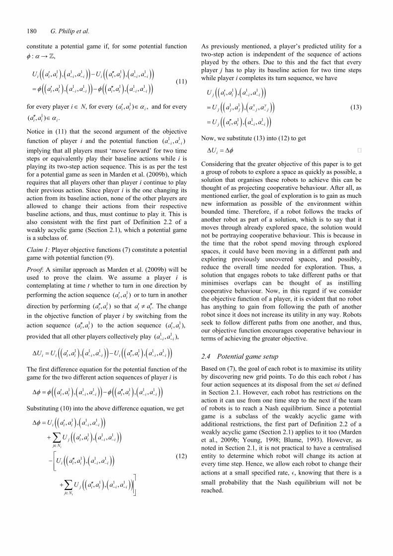
If there are obstacles in the environment, we note a very important limitation of Algorithm 1. As there is a preference (probability 1 − ε) of a robot to keep using its baseline action (i.e., ‘move forward’ with its current pose), it is very likely that it will run into obstacles or walls. Thus, Algorithm 1 must be modified. A simple solution to this problem would be for a robot to change its heading when it encounters an obstacle in front of it even if at that particular moment it is not allowed to perform a turn sequence as dictated by its exploration policy ε. The direction the robot would turn would be the direction that results in the highest utility. This is shown in Algorithm 2. We can immediately perceive the repercussions of this modification as the obstacles would cause robots to change actions more often than ε. In this respect, the presence of obstacles can be considered to have the equivalent effect of increasing ε from the value it was initialised to, which as discussed in Section 2.3 would decrease the probability that the Nash equilibrium will be reached. However, reaching a Nash equilibrium is not our goal here. Our goal is to fully explore a finite space in as little time as possible. In our previous paper, we performed a simulation to compare between the modified potential game algorithm (Algorithm 2) and an uncoordinated algorithm and we demonstrated that the coordination introduced in the algorithm reduces exploration time compared to a completely uncoordinated exploration algorithm. For the same setup used in Philip et
182 G. Philip et al.
al. (2013) consisting of three obstacles and three robots and ε = 0.3, the improvement in exploration time as sRange increases is shown in Figure 3. Though exploration time improves with increasing sRange values, it is evident that improvements are less profound as sRange increases.
Algorithm 2 Modified potential game algorithm
Initialise # of time steps, sRange, and ε
for t ← 1,# of time steps do for all player i ∈ N do Update posi(t), discPtsi(t), and discPts−i(t) if player should turn because of obstacle then Compute 1 1 1( , ) ( , )x
i i i ia a a a∀ ≠
Play 1( , )xi ia a that maximises Ui
else if player should explore based on ε then
Compute Ui, 1( , )xi i ia a α∀ ∈
Play 1( , )xi ia a based on asfi
else Play 1 1( , )i ia a
end if end for end for
3.1 Complexity of Algorithm 2
In this section, we analyse Algorithm 2 to determine its computational complexity. Before we do so, however, we
investigate the computational complexity of Frontier-based exploration algorithms. This gives us a base upon which we can compare and comment on the performance of our algorithm.
As mentioned in Section 1.1, most approaches today use Frontier-based exploration for having a space explored using multiple robots. In Frontier-based exploration, robots explore by repeatedly computing and moving towards Frontiers, which is the boundary that separates known regions from unknown regions (Keidar and Kaminka, 2012). Computing the cost of reaching Frontiers or Frontier detection as it is referred to, involves the use of a deterministic variant of value iteration, a popular DP algorithm (Bellman, 1957; Howard, 1960). In Madani (2002), it was shown that for deterministic Markov decision problems (DMDP), basic value iteration takes Θ(Z2) iterations, where Z denotes the number of states. Thus, it cannot do better than an O(Z2) algorithm in terms of execution time if we just consider the upper bound of its growth rate. In Frontier detection algorithms, the states correspond to the cells in the explored area. Considering that Frontier detection algorithms processes all the states every time it performs Frontier detection, it can be a time consuming process which slows down exploration (Keidar et al., 2012). In fact, even on powerful computers, state-of-the-art Frontier detection algorithms can take a number of seconds to run for every execution of the algorithm, and if a large region is explored, the robot actually has to wait in its spot until the Frontier detection algorithm terminates (Keidar et al., 2012). To make matters worse, there are Frontier-based algorithms such as the algorithm presented in Wurm et al. (2008) that suggest calling Frontier detection every time-step of the coordination algorithm.
Figure 3 Comparison of exploration time of Algorithm 2 for a sRange of 2, 3, and 4 grid points, and ε = 0.3

Cooperative navigation of unknown environments using potential games 183
There are two important points we note about Algorithm 2 before we analyse its runtime. The first point is that Algorithm 2 is a distributed algorithm. Hence, when we make a statement about its computational complexity, we are referring to an instance of its execution on one of the robots. Secondly, as a robot does not have to make a decision when it is forced to play its baseline action, it does not have to compute anything. In fact, it only seldom needs to calculate values. One occasion that it needs to compute values is when it is allowed to update its action as dictated by ε. The other occasion when it needs to compute values is when it needs to avoid an obstacle, and it needs to decide which direction to turn towards. As ε 1 and if we assume an environment with a large open space with few obstacles and few outer walls in comparison to the area of the overall space, robots would be moving straight most of the time with respect to the total time needed for exploration. They would not need to make many decisions resulting in a drastic reduction in the number of computations needed. Considering the aforementioned points, it is only of interest to us to analyse the computational complexity of Algorithm 2 for a robot i that is allowed to update its action at time t, and we proceed bearing this in mind.
As discussed earlier, the argmax operator in the function asfi [equation (14)] selects the two-step action sequence from the two-step action sequence set αi that would give i the most amount of utility or that maximises objective function (7). Based on the actions we defined in the action set Ai and the resulting two-step action sequence set αi that was derived from it, player i has to compute the utility it expects to receive from performing each of the four two-step action sequences to make a decision. It namely has to compute the utility it would receive by playing
1 1 2 1 3 1( , ), ( , ), ( , ),i i i i i ia a a a a a and 4 1( , ).i ia a Figure 4 shows player i contemplating each of the two-step action sequences at time t in a Z × Z grid. The robot is the black box and the arrow on top of it represents the direction it is facing. The two solid dots ahead of the robot represents its predicted positions if it were to play its baseline action for the following two time steps (i.e., 1 1( , )i ia a ). The solid dots to the left, bottom, and right of the robot represents its predicted positions at the end of the second time step after playing 2 1 3 1( , ), ( , ),i i i ia a a a and 4 1( , )i ia a respectively. Recall from Section 2.1.3 that under the framework of the simple forward turn controller, when a robot performs a two-step action sequence that involves a turn, the robot remains in the same position for the first time step. Thus, over the course of a two-step action sequence the position would only change once, and this is why there is only one dot present to the left, bottom, and right of the robot in Figure 4. The circles represent the 360° coverage of the sensor from the future positions, and the range of the sensor, sRange, has been set to 2 grid points. In the objective function (7) for a player, the function f[posi(t + 2), pt] is evaluated for every point pt ∈ gridpts. This leads to Z2 iterations of f[posi(t + 2), pt] as the grid is Z × Z in dimension. Evaluating
f[posi(t + 2), pt] for a particular point pt is not intensive computationally because the majority of the function involves verifying whether or not pt belongs to the set discPtsi(t) or discPts−i(t). This is as simple as maintaining a lookup table in memory in the form of an array and having a simple array indexing operation. Since retrieving a value from memory is very fast, cross-checking pt with already discovered points is an inexpensive operation. In the clauses C1 and C2 in (7), the operations to determine whether pt ∉ discPts−i(t) must be executed first because if it does not hold true, the magnitude function to determine if ||pt − loci(t + 1)|| ≤ sRange is true or if ||pt − loci(t + 2)|| ≤ sRange is true, does not need to be evaluated. Even if the magnitude function is required to be evaluated, the computation needed for it does not have any affect on the runtime order for iterating through all the points. Since there are four two-step actions sequences to be considered, 4Z2 iterations are needed, which is of order Z2. Thus, the runtime order would be O(Z2).
Figure 4 Player i considering each two-step action sequence
If the function f[posi(t + 2), pt] did not have to be evaluated for every point in the grid, the complexity of computing the objective function (7) for a player i for an action sequence
1( , )xi ia a could be reduced. Since the points that have
already been discovered by player i, namely discPtsi(t), are present in the lookup table, the function f[posi(t + 2), pt] does not have to be evaluated for them to determine their contribution to the overall utility of player i. Instead, a very simple operation can be used to query the number of elements in discPtsi(t), which would indicate the utility of player i prior to time t. The problem then becomes to iterate through only a subset of points in the grid that have the potential of increasing player i’s utility in the following two-step action sequence. It would be necessary to at least scan through the points that would be in range of the sensor in the future positions. Since the sensor has a circular coverage, a solution would be to enclose the points that would be covered by the sensor’s range using a square, and
184 G. Philip et al.
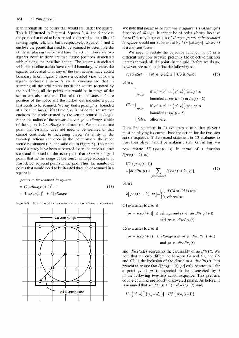
scan through all the points that would fall under the square. This is illustrated in Figure 4. Squares 3, 4, and 5 enclose the points that need to be scanned to determine the utility of turning right, left, and back respectively. Squares 1 and 2 enclose the points that need to be scanned to determine the utility of playing the current baseline action. There are two squares because there are two future positions associated with playing the baseline action. The squares associated with the baseline action have a solid boundary, whereas the squares associated with any of the turn actions have dotted boundary lines. Figure 5 shows a detailed view of how a square encloses a sensor’s radial coverage so that in scanning all the grid points inside the square (denoted by the bold line), all the points that would be in range of the sensor are also scanned. The solid dot indicates a future position of the robot and the hollow dot indicates a point that needs to be scanned. We say that a point pt is ‘bounded at a location loci(t)’ if at time t, pt is inside the square that encloses the circle created by the sensor centred at loci(t). Since the radius of the sensor’s coverage is sRange, a side of the square is 2 ∗ sRange in dimension. We note that one point that certainly does not need to be scanned or that cannot contribute to increasing player i’s utility in the two-step actions sequence is the point where the robot would be situated (i.e., the solid dot in Figure 5). This point would already have been accounted for in the previous time step, and is based on the assumption that sRange ≥ 1 grid point; that is, the range of the sensor is large enough to at least detect adjacent points in the grid. Thus, the number of points that would need to be iterated through or scanned in a square is
2
2
(2 | | 1) 1
4 | | 4 | |
points to be scanned in square
sRange
sRange sRange
= + −
= +
(15)
Figure 5 Example of a square enclosing sensor’s radial coverage
We note that points to be scanned in square is a O(sRange2) function of sRange. It cannot be of order sRange because for sufficiently large values of sRange, points to be scanned in square would not be bounded by M ∗ |sRange|, where M is a constant factor.
We need to restate the objective function in (7) in a different way now because presently the objective function iterates through all the points in the grid. Before we do so, however, we need to define the following set.
{ | 3 is },squareSet pt gridpts C true= ∈ (16)
where,
( )
( )
1 1
1 1
if in , and is ,
bounded at ( 1) or ( 2)3 if in , and is
,bounded at ( 2)
, otherwise
x xi i i i
i i
x xi i i i
i
a a a a pttrue
loc t loc tC a a a a pt
trueloc t
false
⎧ =⎪⎪ + +⎪
= ⎨ ≠⎪⎪ +⎪⎩
If the first statement in C3 evaluates to true, then player i must be playing its current baseline action for the two-step action sequence. If the second statement in C3 evaluates to true, then player i must be making a turn. Given this, we now restate
1( ( 1))ia
i iU pos t + in terms of a function h[posi(t + 2), pt].
( )1
( 1)
( ) [ ( 2), ],
iai i
i ipt squareSet
U pos t
discPts t h pos t pt∈
+
= + +∑ (17)
where
[ ] 1, if 4 or 5 is ( 2),
0, otherwiseiC C true
h pos t pt ⎧+ = ⎨
⎩
C4 evaluates to true if
( 1) and ( 1) and ( ),
i i
i
pt loc t sRange pt discPts tpt discPts t
−− + ≤ ∉ +
∉
C5 evaluates to true if
( 2) and ( 1) and ( ),
i i
i
pt loc t sRange pt discPts tpt discPts t
−− + ≤ ∉ +
∉
and |discPtsi(t)| represents the cardinality of discPtsi(t). We note that the only difference between C4 and C1, and C5 and C2, is the inclusion of the clause pt ∉ discPtsi(t). It is present to ensure that h[posi(t + 2), pt] only equates to 1 for a point pt if pt is expected to be discovered by i in the following two-step action sequence. This prevents double-counting previously discovered points. As before, it is assumed that discPts−i(t + 1) = discPts−i(t), and,
( ) ( )( ) ( )11, , ( 1) .iax
i i i i i i iU a a a a U pos t− −′ ′′− = +
Cooperative navigation of unknown environments using potential games 185
Considering that (17) has to be computed for four two-step actions sequences, a total of 20(|sRange|2 + |sRange|) iterations are needed. This is calculated using (15) as follows.
( )( )
2
2
2
5
5 (2 | | 1) 1
5 4 | | 4 | |
20 | | | |
total iterations points to be scanned in square
sRange
sRange sRange
sRange sRange
= ∗
⎡ ⎤= + −⎣ ⎦
= +
= +
The coefficient 5 above is present rather than 4 because as mentioned earlier there are two future positions associated with playing the baseline action, and so, two squares are required. From the definition of the big O notation, we have
( )( )( )
2
2
20 | | | |
total iterations O sRange sRange
total iterations O sRange
∈ +
⇒ ∈
4 Improved exploration algorithm
This section discusses an improvement to Algorithm 2 in terms of the time taken to explore a space. The improvement stems from each robot predicting the location of every other robot when deciding on a direction to turn. This allows a robot to change its heading to avoid exploring the same areas as other robots, and as a result achieve a greater degree of coordination. The basis of the prediction is that when a robot i is allowed to perform a turn sequence based on its exploration rate ε, it can be reasonably sure that every other robot will play their baseline action or move forward for the two time steps required to complete i’s turn. In fact, the prediction becomes more accurate the smaller ε is set to because robots will turn less often, and thus when a robot is allowed to turn it can be reasonably sure that other robots will not turn. A robot that is deciding to turn needs to know the heading and the location of every other robot (i.e., pos−i(t)) in the time step it is deciding on turning on so that it can predict the locations of all the robots in the two time steps it will take to perform its turn (i.e., ˆ ( 1)ipos t− + and ˆ ( 2)ipos t− + ). Taking into account the aforementioned, we now redefine the objective function of a player i in (7) as
( ) ( )( )( )
[ ]
1
1 1 1, , ,
ˆ( 1), ( 1)
ˆ( 2), ( 2),
i
xi i i i i
ai i i
i ipt gridpts
U a a a a
U pos t pos t
f pos t pos t pt
− −
−
−∈
= + +
= + +∑
where
[ ]ˆ( 2), ( 2),
1, if ( )1, if 1 is 1, if 2 is 0, otherwise
i i
i
f pos t pos t pt
pt discPts tC trueC true
−+ +
∈⎧⎪⎪= ⎨⎪⎪⎩
Condition C1 evaluates to true if
1 || ( 1) || andˆ( ) and || ( 1) ||
ˆ and || ( 2) || .
i
i i
i
C pt loc t sRangept discPts t pt loc t sRange
pt loc t sRange− −
−
⇐ − + ≤
∉ − +
− +
Condition C2 is the same as C1, except the first clause of the condition is
ˆ|| ( 2) || .ipt loc t sRange− +
In comparison to (7), equation (18) uses 1 1( , )i ia a− − rather than ( )i ia a− −′ ′′− signifying that the objective function is calculated under the assumption that other robots move forward in the following two time steps. The clause
ˆ ˆ|| ( 1) || or || ( 2) || .i ipt loc t sRange pt loc t sRange− −− + − + evaluate to true if pt is not in range of any of the robots aside from robot i in the respective time step. It can be seen that in maximising (18), a robot i avoids heading in a direction that it predicts other robots are going to move towards.
Equation (18) is the objective function for any robot i that is able to change its action at a time t. For every other robot that is not allowed to change its action at time t from its baseline action (i.e., moving forward) as dictated by ε, its predicted utility for the two-step action sequence that follows is calculated using (7).
We need to introduce new rules for updating discPtsi(t) and ˆ ( )idiscPts t− that is consistent with the objective function (18). As with the previous objective function (7), at the beginning of a time step posi(t) is updated, except if a robot i is in the middle of a turn sequence in which case it needs to update pos−i(t) as well. Then discPtsi(t) and
ˆ ( )idiscPts t− are updated. However, depending on whether a robot has the option of performing a turn sequence or not at a time t as dictated by _, we differentiate how discPtsi(t) is updated. Based on C1 and C2 in (18), a robot i that has the option of performing a turn sequence at a time t does not expect to increase its utility by discovering new grid points in the following two time steps if it predicts those grid points would be discovered by other robots in those two times steps. Thus, to be consistent with the prediction, i must ensure those grid points do not get included in discPtsi(t) when it updates the set after taking an action. This is reflected in (19).
186 G. Philip et al.
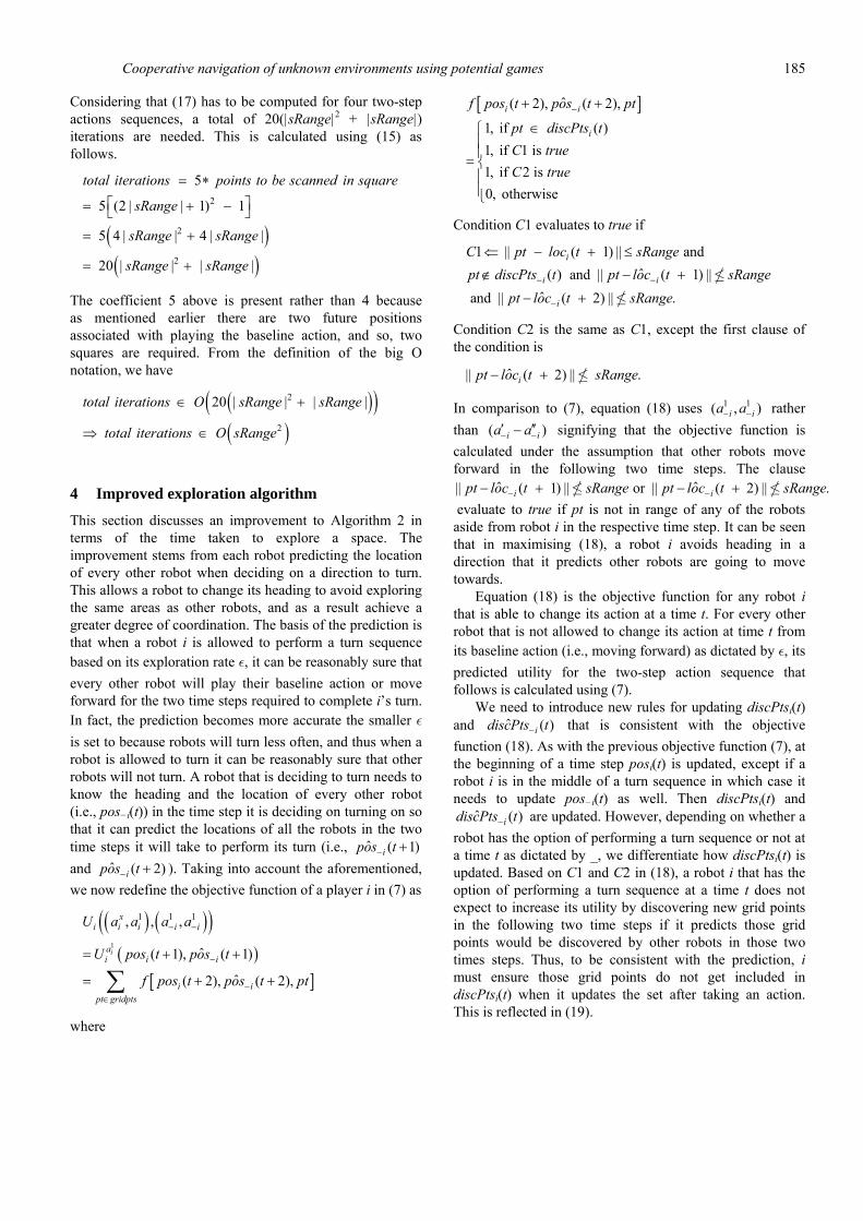
Figure 6 Comparison of exploration time of Algorithm 2 and improved algorithm
If a robot i has the option of performing a turn sequence at time t, discPtsi(t) is updated as follows in the following two time steps.
( ) { | 5} ( 1)i idiscPts t pt gridpts C discPts t= ∈ −∪ (19)
where
5 || ( 1) || andˆ ˆ( ) and || ( ) ||
i
i i
C pt loc t sRangept discPts t pt loc t sRange− −
⇐ − + ≤
∉ −
If on the other hand a robot i can only play its baseline action, discPtsi(t) is updated as follows in the following two time steps.
( ) { | 6} ( 1)i idiscPts t pt gridpts C discPts t= ∈ −∪
where
6 || ( ) || and ( 1)i iC pt loc t sRange pt discPts t−⇐ − ≤ ∉ −
Finally, discPts−i(t) is updated for all robots as follows.
{ }( ) | ( )i
i jj N
discPts t pt gridpts pt discPts t−∈
= ∈ ∈∪
Claim 2: Player objective functions (18) constitute a potential game with potential function (9).
The proof for Claim 2 is identical to the proof of Claim 1. To assess the effect of using (18) on exploration time, we replace the objective function used in Algorithm 2 [i.e., (7)] with (18) and use the new rules for updating discPtsi(t) and discPts−i(t) as discussed in this section. We will refer to this modified algorithm as the Improved Algorithm. We then simulate the Improved Algorithm for the test environment introduced in Philip et al. (2013) with sRange set to 2 grid pts and ε set to 0.1. The simulation is run for 2,000 time
steps and averaged over 20 games. Figure 6 compares the performance of Algorithm 2 with the Improved Algorithm. It can be seen that the Improved Algorithm discovers more grid points from the 200 th to the 700 th time step, but in terms of the total time it takes to explore the whole space there is no difference between the two algorithms. However, it can be argued that if there is only a limited time given to explore the space (e.g., 400 time steps), then the Improved Algorithm would explore more of the space than Algorithm 2. On the contrary it is important to note that with the Improved Algorithm, a robot that is performing a turn sequence requires more information from the other robots compared to Algorithm 2. Specifically, it needs pos−i(t), which includes both the heading and location of the other robots. Furthermore, as before, the robot needs to know all the grid points discovered by other robots for it to compute discPts−i(t). Thus, the improvement in exploration time of improved algorithm comes at the expense of more information having to be shared among the robots.
5 Conclusions
In this paper we investigated exploring 2-D spaces using potential games rather than conventional Frontier-based DP methods. The objective function of a player and the game’s potential function were defined in terms of the discovery of unexplored grid points by robots, and the definition of a potential game was extended for a two-step action sequence. Based on the objective function of a player and incorporating the simple forward turn controller, we devised an algorithm for exploration, which was then modified for a bounded environment with obstacles. The computational complexity of the resulting algorithm was analysed to be O(sRange2), where sRange is the range of a sensor on a robot. Finally, an improved exploration algorithm that is
Cooperative navigation of unknown environments using potential games 187
based on predicting future locations of robots was discussed in Section 4.
A simulation using three robots and three obstacles indicated that the Improved Algorithm was able to improve the exploration of the environment for a period of time, but the total time for exploration did not differ from the modified potential game algorithm. However, the improvement in exploration time comes at the expense of more information having to be shared among the robots.
To account for environments that pose severe bandwidth constraints on communications between robots such as in AUV platforms, future work will involve developing a game in which robots do not communicate with their neighbours at every time step. Furthermore, the suitability of integrating the exploration method discussed in this paper with Frontier-based DP methods would be an interesting research direction.
References Asmar, D. and Shaker, S. (2012) ‘2D occupancy-grid SLAM of
structured indoor environments using a single camera’, Int. J. Mechatronics and Automation, Vol. 2, No. 2, pp.1009–1014.
Bellman, R.E. (1957) Dynamic Programming, Princeton University Press, Princeton, NJ.
Blume, L. (1993) ‘The statistical mechanics of strategic interaction’, Games and Economic Behaviour, Vol. 5, No. 3, pp.387–424.
Blume, L. (1996) Population Games, Game Theory and Information 9607001, EconWPA, Munich, Germany.
Burgard, W., Moors, M., Fox, D., Simmons, R. and Thrun, S. (2000) ‘Collaborative multi-robot exploration’, Proc. IEEE Int. Conf. Robot. Autom. (ICRA), pp.476–481.
Castellanos, J., Montiel, J.M.M., Neira, J. and Tardos, J.D. (2001) ‘The SPmap: a probabilistic framework for simultaneous localization and map building’, IEEE Trans. Robot. Autom., Vol. 15, No. 2, pp.125–137.
Dissanayake, G., Durrant-Whyte, H. and Bailey, T. (2000) ‘A Computationally efficient solution to the simultaneous localization and map building (SLAM) problem’, Proc. IEEE Int. Conf. Robot. Autom. (ICRA), pp.1009–1014.
Fabrikant, A., Jaggard, A.D. and Schapira, M. (2010) ‘On the structure of weakly acyclic games’, Proceedings of the Third International Conference on Algorithmic Game Theory, SAGT ‘10, pp.126–137, Springer-Verlag, Berlin, Heidelberg, ISBN 3-642-16169-3, 978-3-642-16169-8.
Howard, R.A. (1960) Dynamic Programming and Markov Processes, MIT Press and Wiley, Cambridge, Massachusetts, USA.
Keidar, M. and Kaminka, G.A. (2012) ‘Robot exploration with fast Frontier detection: theory and experiments’, Proc. 11th Intl. Conf. Auton. Agents Multiagent Sys., Vol. 1, pp.113–120.
Lindsay, J. (2011) Nonholonomic Consensus in Cooperative Robotics: A Game Theoretical Approach, Masters thesis, Royal Military College of Canada, Kingston, Ontario.
Lu, X. (2012) Multi-Agent Reinforcement Learning in Games, PhD thesis, Carleton University, Ottawa, Ontario.
Madani, O. (2002) ‘Polynomial value iteration algorithms for deterministic MDPs’, Proceedings of the Eighteenth conference on Uncertainty in Artificial Intelligence, pp.311–318.
Marden, J.R. and Shamma, J.S. (2007) ‘Autonomous vehicle target assignment: a game theoretical formulation’, ASME Journal of Dynamic Systems, Measurement, and Control, Vol. 129, No. 5, pp.584–596.
Marden, J.R., Young, H.P., Arslan, G. and Shamma, J.S. (2009a) ‘Payoff-based dynamics for multiplayer weakly acyclic games’, SIAM J. Control Optim., Vol. 48, No. 1, pp.373–396.
Marden, J.R., Arslan, G. and Shamma, J.S. (2009b) ‘Cooperative control and potential games’, Systems, Man, and Cybernetics, Part B: Cybernetics, IEEE Transactions on, Vol. 39, No. 6, pp.1393–1407.
Philip, G., Givigi, S. and Schwartz, H. (2013) ‘Multi-robot exploration using potential games’, Proc. IEEE Intl. Conf. Mechatronics Autom. (ICMA).
Sun, Y., Zhang, J., Wang, S. and Jiao, W. (2012) ‘A real-time intelligent route planning method in geomagnetic navigation’, Int. J. Mechatronics and Automation, Vol. 2, No. 2, pp.125–131.
Wadhams, P. (2012) ‘The use of autonomous underwater vehicles to map the variability of underice topography’, Ocean Dynamics, Vol. 62, No. 3, pp.439–447.
Wong, R.H., Xiao, J., Joseph, S.L. and He, S. (2013) ‘A mixed model data association for simultaneous localisation and mapping in dynamic environments’, Int. J. Mechatronics and Automation, Vol. 3, No. 1, pp.1–15.
Wurm, K.M., Stachniss, C. and Burgard, W. (2008) ‘Coordinated multi-robot exploration using a segmentation of the environment’, Intelligent Robots and Systems, IROS, IEEE/RSJ International Conference on, pp.1160–1165.
Young, H.P. (1998) Strategy and Social Structure, Princeton University Press, Princeton, NJ.


![Convolutional Neural Network-Based Robot Navigation Using ... · problem. Decades later, Hadsell et al. [12] developed a similar system for ground robot navigation in unknown environments](https://img.dokumen.tips/doc/110x75/5f15d50ea746d01e9417aaf3/convolutional-neural-network-based-robot-navigation-using-problem-decades-later.jpg)