Dynamic Flood Risk Conditional on Climate Variation:

A New Direction for Managing Hydrologic Hazards in the 21st Century? 

Upmanu LallDept. of Earth & Environmental Engineering

& Intl. Research Institute For Climate Prediction

Columbia University

Co-authors: G. Pizarro, S. Arumugam and S. Jain

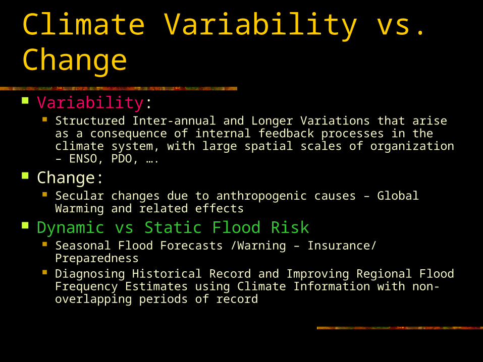
Climate Variability vs. Change Variability:

Structured Inter-annual and Longer Variations that arise as a consequence of internal feedback processes in the climate system, with large spatial scales of organization – ENSO, PDO, ….

Change: Secular changes due to anthropogenic causes – Global Warming

and related effects

Dynamic vs Static Flood Risk Seasonal Flood Forecasts /Warning – Insurance/ Preparedness Diagnosing Historical Record and Improving Regional Flood

Frequency Estimates using Climate Information with non-overlapping periods of record

Outline

Context through Sacramento Floods Nature of Nonstationarity:

Washington Example Cane-Zebiak Model Inferences

Prediction in the US West E[Annual Max Flood] for the upcoming year Reconstruction of Past floods

Local Likelihood Method for Quantile Forecasts

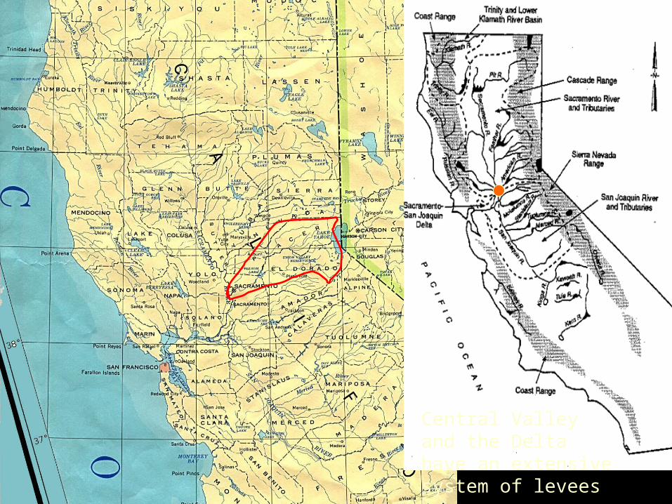
Central Valley and the Delta have an extensive system of levees

19th century : Personal Levees, Rebuild to higher than last biggest

20th century : Dams, Levees, bypass, Heavily Federally Subsidized

21st century : ??

American River at Fair Oaks - Ann. Max. Flood

020,00040,00060,00080,000

100,000120,000140,000160,000180,000

1900 1920 1940 1960 1980 2000

Year

An

n M

ax

Flo

w

100 yr flood estimated from 21 & 51 yr moving windows

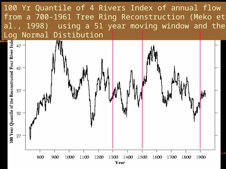
100 Yr Quantile of 4 Rivers Index of annual flow from a 700-1961 Tree Ring Reconstruction (Meko et al., 1998) using a 51 year moving window and the Log Normal Distibution

Identifying Variability & co-variation with climate indices

Moving Window Analyses Mean, Variance, T-year flood “Arrival Rate” – Non-homogeneous Poisson Process

Correlations and Nonparametric Regression Spectrum (Frequency Domain)

Multivariate Spectrum Composites of Climate Fields for High/Low

Flood Years

Historical Record for the Blacksmith Fork river (1914-96)Historical Record for the Blacksmith Fork river (1914-96)

1920 1930 1940 1950 1960 1970 1980 1990

200

600

1000

1400

(a)

year

Flo

od (

cfs)

0.00 0.05 0.10 0.15 0.20 0.25 0.30 0.35 0.40 0.45 0.50

0.1

0.2

0.3

0.4

0.5

0.6

0.7

0.8

0.9

1.0

(b)

Frequency (/yr)

Sca

led

Spe

ctru

m

1920 1930 1940 1950 1960 1970 1980 1990

160

170

180

190

200

210

220

230

240

(c)

year

Day

of

Wat

er y

r

160 170 180 190 200 210 220 230 240

200

600

1000

1400

(d)

Day of Water yr

Flo

od (

cfs)

BFR Flood w/10yr smooth Spectrum

Annual Max: Day of Water year Flood magnitude vs. timing

Jain & Lall, 2000

Blacksmith Fork, Hyrum, UT

Analyses of Flood Statistics using a 30 year Moving Window

From Jain and Lall (2000)

100 yr flood (LN)

Var(log(Q))Mean(log(Q))

Flood mean given DJF NINO3 and PDO

NINO3 PDO

Flood Variance given DJFNINO3 and PDO

NINO3PDO

Derived using weighted local regression with 30 neighbors

Correlations:

Log(Q) vs DJF NINO3 -0.34 vs DJF PDO -0.32

Jain & Lall, 2000

1920 1940 1960 1980 2000

year

5000

10000

20000

40000

Ann

ual M

axim

um F

lood

(cf

s)

30-year smooth

1920 1940 1960 1980 2000

year

-0.2

0.0

0.2

0.4

0.6

0.8

NIN

O3

Inde

x

-1.5

-1.0

-0.5

0.0

0.5

1.0

PD

O I

ndex

Similkameen River near Nighthawk, Washington, 1911-98

NINO3 NINO3|PDO

PDO PDO|NINO3

Flood -0.39 -0.27 -0.44 -0.33

Correlations

Jain & Lall, 2001

1920 1940 1960 1980 2000

Year

020

4060

8010

0

Per

cen

t p

rob

abili

ty o

f ex

ceed

ance

10%

33%

67%

90%

Floods

as a

Non-homogeneous Poisson Process:

Prob. Of Exceedance of flood (t) =

“rate of arrival” (t)

= “rate of Poisson Process of exceedances”

Kernel Estimate using a 30 year moving window

Jain & Lall, 2001

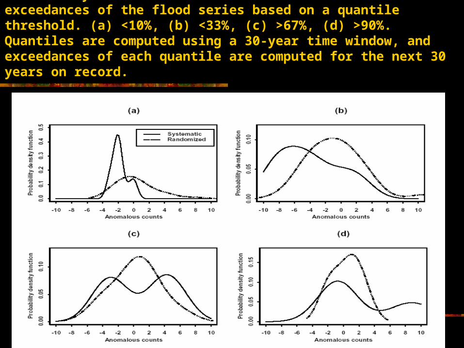
Probability distribution of the number of anomalous exceedances of the flood series based on a quantile threshold. (a) <10%, (b) <33%, (c) >67%, (d) >90%. Quantiles are computed using a 30-year time window, and exceedances of each quantile are computed for the next 30 years on record.

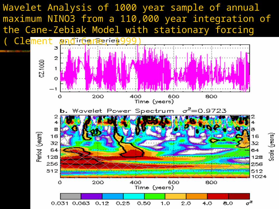
Wavelet Analysis of 1000 year sample of annual maximum NINO3 from a 110,000 year integration of the Cane-Zebiak Model with stationary forcing ( Clement and Cane, 1999)

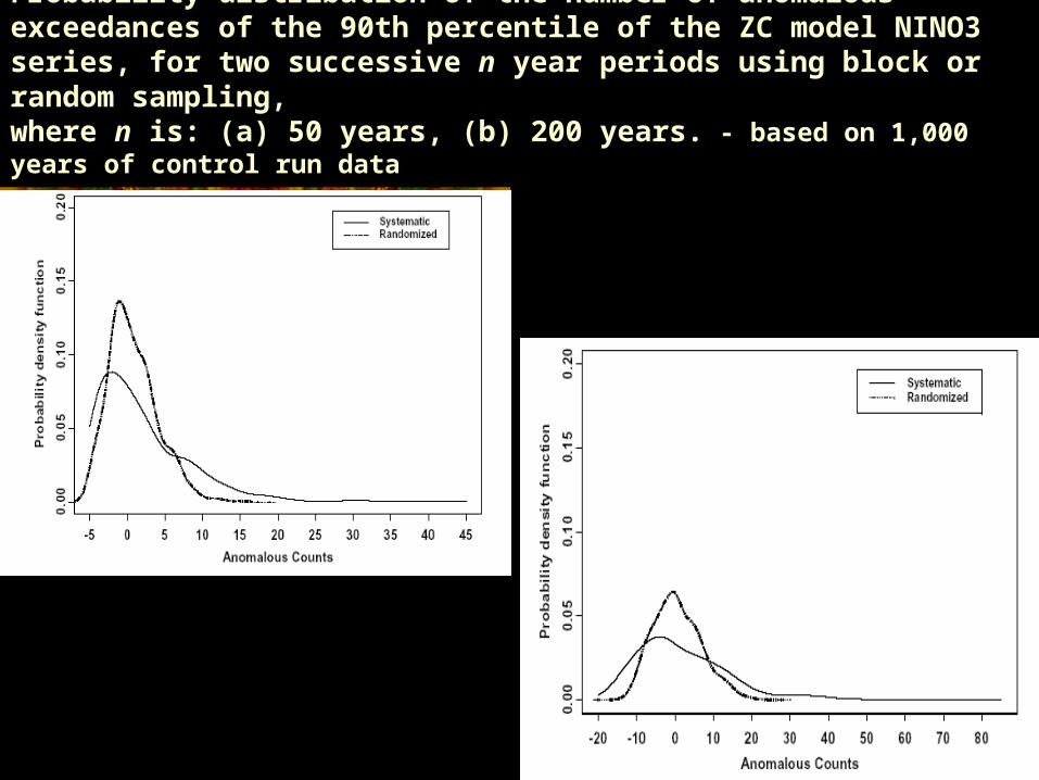
Probability distribution of the number of anomalous exceedances of the 90th percentile of the ZC model NINO3 series, for two successive n year periods using block or random sampling, where n is: (a) 50 years, (b) 200 years. - based on 1,000 years of control run data

Ann. Max. Flood Seasonality in the West

3133

1

3

333 3

33

33

3

43

44

444

1111

14

3

31

11111

14

1344444

44444444

4

44

44

422

4

11131

1

2

1

11111

1

13

31 11

22

2211

2 3

222 22 122 22222 12

2 2222 22 12 22 1222222

2 12 12222 12 24 11Pizarro & Lall, 2002

Partial CorrelationsPizarro & Lall, 2002

Flood with NINO3 | PDO Flood with PDO | NINO3

Predictors Considered (All Jan-Apr)

First 2 PCs of the average SST and first 2 PCs of the Jan-Apr change of the Pacific SST over

Lat (5S,60N) and Long(60E, 60W)

NINO3 Average and Change

PDO Average and Change

Projection Pursuit Regression

Goal: Fit the multivariate model

y = f(x) + e f(x) is approximated by univariate nonparameteric functions

applied to linear combinations of x For a single response:

Sj(.) = Univariate Regression = Supersmoother Weighted unexplained variance reduction across all response

variables used to choose # of basis functions Cross-validation (Randomly drop 10% of data 100 times) used

to choose predictors

From Friedman & Stuetzle, 1981

εSαyM

j

Tjj

10 xα

PPR Implementation Normalize Log(Flow) Data at each site in cluster

Try several PPR models varying the number of basis functions (M …. 1), and Predictor Combinations.

Choose m <=M basis functions as breakpoint of unexplained variance vs M for each predictor set

Choose Predictor Combination using cross validated average error variance reduction across all sites in cluster

From Cross-validation runs estimate: Unexplained variance per station Hindcasts/Forecasts for each station Approx. Confidence interval per station

Hindcast - Examples

(6b) Local Likelihood

0

10000

20000

30000

40000

50000

60000

1930 1940 1950 1960 1970 1980 1990 2000

Year

Qu

anti

les

(Cfs

)

p=0.1 Unconditionalp=0.5 Unconditionalp=0.9 UnconditionalObserved flowsp=0.1 Conditionalp=0.5 Conditionalp=0.9 Conditional

Local Likelihood: Annual Conditional Flood Forecasts

Arumugam and Lall, 2003Conditional pdf with parameters (Xt). )( ttQf X

)()( ttt XX )θ(X

m

kktkjkt xx

10 )()( X

m

kktxkjxkt

1)(0)( X

otherwise 0

1|| if 1

)21()(

kkjum

kkjutjw X

khkjxktx

kju

n

tj

jttttQftjwttCV

1)ˆ ;(log()()ˆ,ˆ( )(X-θXXh)(X-θ

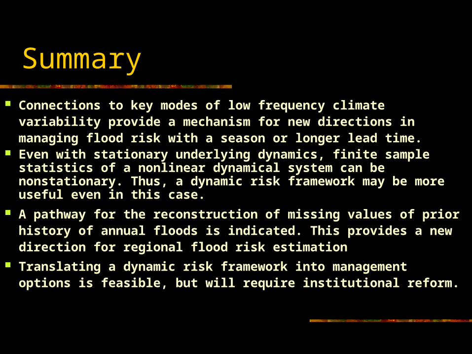
Summary Connections to key modes of low frequency climate variability provide

a mechanism for new directions in managing flood risk with a season or longer lead time.

Even with stationary underlying dynamics, finite sample statistics of a nonlinear dynamical system can be nonstationary. Thus, a dynamic risk framework may be more useful even in this case.

A pathway for the reconstruction of missing values of prior history of annual floods is indicated. This provides a new direction for regional flood risk estimation

Translating a dynamic risk framework into management options is feasible, but will require institutional reform.