INL/EXT-15-36758

Light Water Reactor Sustainability Program

Dynamic Event Tree Advancements

and Control Logic Improvements

September 2015

DOE Office of Nuclear Energy

DISCLAIMERThis information was prepared as an account of work sponsored by an agency of the U.S. Government. Neither the U.S. Government nor any agency thereof, nor any of their employees, makes any warranty, expressed or implied, or assumes any legal liability or responsibility for the accuracy, completeness, or usefulness, of any information, apparatus, product, or process disclosed, or represents that its use would not infringe privately owned rights. References herein to any specific commercial product, process, or service by trade name, trade mark, manufacturer, or otherwise, do not necessarily constitute or imply its endorsement, recommendation, or favoring by the U.S. Government or anyagency thereof. The views and opinions of authors expressed herein do notnecessarily state or reflect those of the U.S. Government or any agency thereof.

INL/EXT-15-36758

Light Water Reactor Sustainability Program

Dynamic Event Tree Advancements and Control Logic Improvements

Andrea Alfonsi, Cristian Rabiti, Joshua Cogliati, Diego Mandelli, Sonat Sen, Robert Kinoshita, Congjian Wang, Paul Talbot, Dan Maljovec, Andrew Slaughter, Curtis

Smith

September 2015

Idaho National LaboratoryIdaho Falls, Idaho 83415

http://www.inl.gov/lwrs

Prepared for theU.S. Department of EnergyOffice of Nuclear Energy

Under DOE Idaho Operations OfficeContract DE-AC07-05ID14517

ii

EXECUTIVE SUMMARY

The RAVEN code has been under development at the Idaho National Laboratory since 2012. Its main goal is to create a multi-purpose platform for the deploying of all the capabilities needed for Probabilistic Risk Assessment, uncertainty quantification, data mining analysis and optimization studies. RAVEN is currently equipped with three different sampling categories: Forward samplers (Monte Carlo, Latin Hyper Cube, Stratified, Grid Sampler, Factorials, etc.), Adaptive Samplers (Limit Surface search, Adaptive Polynomial Chaos, etc.) and Dynamic Event Tree (DET) samplers (Deterministic and Adaptive Dynamic Event Trees).

The main subject of this report is to show the activities that have been recently accomplished:

- Migration of the RAVEN/RELAP-7 control logic system into MOOSE, and - Development of advanced dynamic sampling capabilities based on the Dynamic Event

Tree approach.In order to provide to all MOOSE-based applications a control logic capability, in this Fiscal

Year a migration activity has been initiated, moving the control logic system, designed for RELAP-7 by the RAVEN team, into the MOOSE framework.

The second and most important subject of this report is about the development of a Dynamic Event Tree (DET) sampler named “Hybrid Dynamic Event Tree” (HDET) and its Adaptive version “Adaptive Hybrid Dynamic Event Tree” (AHDET). Among different types of uncertainties, it is possible to discern them two main types: aleatory and epistemic. The classical Dynamic Event Tree is in charge of treating the first type of uncertainties (i.e., aleatory); the dependence of the probabilistic risk assessment and analysis on the epistemic uncertainties istreated by an initial Monte Carlo sampling (MCDET). For each Monte Carlo sample (i.e., sampling of the set of the epistemic variables), a DET analysis is run (in total, N trees). The Monte Carlo employs a pre-sampling of the input space characterized by epistemic uncertainties. The consequent Dynamic Event Tree performs the exploration of the aleatory space.

In the RAVEN code, a more general approach has been developed, not limiting the exploration of the epistemic space through a Monte Carlo method but using all the forwardsampling strategies currently available in RAVEN. The user can combine a Latin Hyper Cube, Grid, Stratified and Monte Carlo sampling in order to explore the epistemic space, without any limitation. From this pre-sampling, the Dynamic Event Tree sampler starts its aleatory space exploration.

The Dynamic Event Tree is a good fit to develop a goal oriented sampling strategy. The DET is used to drive a Limit Surface search. The methodology that has been developed by the authors last year performs a Limit Surface search in the aleatory space only. This report documents how this approach has been extended in order to consider the epistemic space interacting with the Hybrid Dynamic Event Tree methodology.

iii

CONTENTS

EXECUTIVE SUMMARY .......................................................................................................................... ii FIGURES...................................................................................................................................................... v TABLES ...................................................................................................................................................... vi ACRONYMS..............................................................................................................................................vii 1. INTRODUCTION.............................................................................................................................. 1

1.1 Document structure ............................................................................................................... 2 2. RAVEN, MOOSE and RELAP-7....................................................................................................... 3

2.1 RAVEN ................................................................................................................................. 3 2.1.1 Control logic system ........................................................................................... 3 2.1.2 RAVEN: UQ/PRA and statistical framework..................................................... 5

2.2 MOOSE................................................................................................................................. 6 2.3 RELAP-7 ............................................................................................................................... 7

3. RAVEN/RELAP-7 control logic system and initial migration throughout MOOSE......................... 9 3.1 RAVEN and Control Logic ................................................................................................... 9 3.2 Implementation.................................................................................................................... 10 3.3 Control Example.................................................................................................................. 11

4. Dynamic Event Tree concept in RAVEN......................................................................................... 15 5. The Hybrid Dynamic Event Tree method ........................................................................................ 17 6. The Adaptive Hybrid Dynamic Event Tree...................................................................................... 20

6.1 Limit Surface....................................................................................................................... 20 6.2 Reduced Order Models........................................................................................................ 21 6.3 Adaptive Dynamic Event Tree ............................................................................................ 22 6.4 Adaptive Hybrid Dynamic Event Tree methodology.......................................................... 25

6.4.1 AHDET: Epistemic uncertainties not projected in the LS space ...................... 26 6.4.2 AHDET: Epistemic uncertainties projected in the LS space............................. 27

7. Proof of concept: PRA analysis on a simplified PWR-like model. .................................................. 29

iv

7.1 PWR system. ....................................................................................................................... 29 7.2 Plant Mechanistic Modeling................................................................................................ 31 7.3 SBO Scenario. ..................................................................................................................... 32 7.4 Aleatory uncertainties.......................................................................................................... 32 7.5 Epistemic uncertainties........................................................................................................ 33

7.5.1 Epistemic uncertainties used in HDET sampling strategy ................................ 33 7.5.2 Epistemic uncertainties used in AHDET sampling strategy ............................. 33

7.6 Stochastic model.................................................................................................................. 34 7.6.1 Stochastic model: Aleatory uncertainties. ......................................................... 34 7.6.2 Stochastic model: Epistemic uncertainties. ....................................................... 35

7.7 Results ................................................................................................................................. 36 7.7.1 SBO scenario analyzed through HDET methodology ...................................... 37 7.7.2 SBO scenario analyzed through AHDET methodology.................................... 39

8. Conclusions ...................................................................................................................................... 43 REFERENCES ........................................................................................................................................... 44

v

FIGURES

Figure 1 - RAVEN simulation controller scheme......................................................................................... 4 Figure 2 – RAVEN framework layout. ......................................................................................................... 5 Figure 3 – RELAP-7 nodalization of an AP1000 demo case........................................................................ 8 Figure 4 – Control Logic system: Old and New scheme. ........................................................................... 10 Figure 5 - Example diffusion problem without (left) and with (right) control logic activation.................. 14 Figure 6 - Dynamic Event Tree conceptual flow........................................................................................ 15 Figure 7 - Epistemic uncertainties’ treatment with basic Dynamic Event Tree method............................. 18 Figure 8 – Hybrid Dynamic Event Tree conceptual scheme ...................................................................... 19 Figure 9 - A-posteriori Limit Surface generated from standard DET......................................................... 22 Figure 10 - Adaptive Dynamic Event Tree Flow Chart.............................................................................. 24 Figure 11 - AHDET: Epistemic uncertainties not projected in the LS space. ............................................ 26 Figure 12 – Example of sheaf of LSs at different levels of an epistemic uncertain parameter................... 27 Figure 13 - AHDET: Epistemic uncertainties active part of the LS search process. .................................. 27 Figure 14 - Scheme of the TMI PWR benchmark. ..................................................................................... 30 Figure 15 - Scheme of the electrical system. .............................................................................................. 30 Figure 16 - PWR RELAP-7 nodalization. .................................................................................................. 31 Figure 17 - HDET clad temperature evolution. .......................................................................................... 37 Figure 18 - HDET cold leg flow velocity evolution. .................................................................................. 38 Figure 19 – HDET histogram maximum fuel temperature. ........................................................................ 38 Figure 20 – HDET histogram maximum clad temperature......................................................................... 39 Figure 21 - Clad Temperature evolution for Core Channel 1 and 2. .......................................................... 40 Figure 22 - Pump Head evolution. .............................................................................................................. 40 Figure 23 - Limit Surface found by the AHDET methodology on the PWR SBO scenario....................... 41 Figure 24 - Limit Surface 2D projection: Combined effect of Power and DGs recovery time. ................. 42 Figure 25 - Limit Surface 2D projection: Combined effect of Failure Temperature and DGs recovery time.42

vi

TABLES

Table 1 - Source code example: ExampleControl.h.................................................................................... 12 Table 2 - Source code example: ExampleControl.C................................................................................... 12 Table 3 - Python function for newly developed MOOSE control logic system ......................................... 14 Table 4 - Epistemic Sampling settings........................................................................................................ 36

vii

ACRONYMS

CDF Cumulative Distribution Function

DOE Department of Energy

DG Diesel generator

DET Dynamic Event Tree

ET Event-Tree

GUI Graphical User Interface

HDET Hybrid Dynamic Event Tree

AHDET Adaptive Hybrid Dynamic Event Tree

IE Initiating Event

INL Idaho National Laboratory

LS Limit Surface

LWR Light Water Reactor

LWRS Light Water Reactor Sustainability

MC Monte-Carlo

MOOSE Multi-physics Object-Oriented Simulation Environment

NPP Nuclear Power Plant

NEAMS Nuclear Energy Advanced Modeling and Simulation

PDF Probability Distribution Function

PRA Probabilistic Risk Assessment

PWR Pressurized Water Reactor

R&D Research and Development

RAVEN Risk Analysis in a Virtual Environment

RISMC Risk Informed Safety Margin Characterization

ROM Reduced Order Model

TH Thermal-Hydraulics

UQ Uncertainty Quantification

1

Dynamic Event Tree advancements and control logic1. INTRODUCTION

RAVEN [1,2,3,4] (Risk Analysis in a Virtual ENviroment), under the combined support of the Nuclear Energy Advanced Modeling and Simulation (NEAMS) and Light Water Reactor Sustainability (LWRS) programs, is increasing its capabilities to perform stochastic analysis of dynamic systems. This supports the goal of providing the tools needed by the Risk Informed Safety Margin Characterization (RISMC) path-lead [5] under the Department of Energy (DOE) LWRS program. In particular, the development of RAVEN in conjunction with the thermal-hydraulic code RELAP-7 [6], will allow the deployment of advanced methodologies for nuclear power plant (NPP) safety analyses at the industrial level. The investigation of accident scenarios in a probabilistic environment for a complex system (i.e. NPPs) is not a minor task. The complexity of such systems and a large quantity of stochastic parameters lead to demanding computational requirements (several CPU/hour). Moreover, high consequence scenarios are usually located in low probability regions of the input space, making RISMC-like types of analysis even more computational demanding.

This extreme need for computational power leads to the necessity to investigate methodologies that reduce the overall computational cost either by increasing effectiveness of the global exploration of input space, or by focusing on regions of interest (e.g. failure/success boundaries, etc.). Several publications [7,8,9,10] of the authors described the capability of RAVEN to perform the exploration of the uncertain domain (probabilistic space) through the support of the well-known Dynamic Event Tree (DET) approach [11] and its evolution, the Adaptive Dynamic Event Tree (ADET) method.

The main focus of this document is to report the activities that have been done in order to:

1. Start the migration of the RAVEN/RELAP-7 control logic system into MOOSE [12],and

2. Develop advanced dynamic sampling capabilities based on the Dynamic Event Tree approach

In order to provide to all MOOSE-based applications a control logic capability, during this Fiscal Year (FY) a migration activity has been initiated, moving the control logic system, designed for RELAP-7 by the RAVEN team, into the MOOSE framework. In this document, a brief explanation of what has been done is reported.

The second and most important subject of this report is about the development of a Dynamic Event Tree (DET) sampler named “Hybrid Dynamic Event Tree” (HDET) and its Adaptive variant “Adaptive Hybrid Dynamic Event Tree” (AHDET). These methodologies and theirimplementations, in the RAVEN code, are discussed in this document. In order to show the effectiveness of these newer methods, a Station Black Out (SBO) scenario for a Pressurized Water Reactor, using RELAP-7 code, has been employed. The HDET and AHDET approachesare used to focus the exploration of the input space toward the computation of the failure probability of the system (i.e. clad failure), under the presence of epistemic uncertainties.

2

1.1 Document structure

This report is organized in 6 additional sections:

Section 2 provides a brief overview of MOOSE, RELAP-7 and RAVEN;

Section 3 briefly recalls structure of the current RAVEN/RELAP-7 control logic system and describes its migration into MOOSE;

Section 4 describes the concept of the DET methodology;

Section 5 reports the new Hybrid Dynamic Event Tree (HDET) methodology;

Section 6 describes the Adaptive Hybrid Dynamic Event Tree (AHDET) method and its implementation in RAVEN;

Section 7 is focused on the analysis performed on the PWR SBO;

Section 8 draws conclusions.

3

2. RAVEN, MOOSE AND RELAP-7

As easily inferable from the Introduction section, the activities here reported have been done using/developing three different platforms: 1) MOOSE, for the control logic migration; 2) RAVEN for the HDET and AHDET methods’ development and 3) RELAP-7 for testing the HDET methodologies. This section describes a general description of these tools.

2.1 RAVEN

RAVEN has been developed in a highly modular and pluggable way in order to enable easy integration of different programming languages (i.e., C++, Python) and coupling with any single and multi-physics code. The RAVEN project is composed of three main software systems that can operate either in coupled or stand-alone mode:

Control logic system

Graphical User Interface

RAVEN: UQ/PRA and Statistical framework

The Graphical User Interface is not crucial for the purpose of this report. For this reason, attention is focused on the control logic system and the probabilistic and parametric framework.

It is important to mention that what now is generally referred as RAVEN is represented by the RAVEN UQ/PRA and Statistical framework; this portion represents the most important and core of the RAVEN environment capabilities.

2.1.1 Control logic system

One of the RAVEN tasks is to act as controller of the RELAP-7 simulation while simulation is running. Such control action is performed using two sets of variables [13]:

Monitored variables: set of observable parameters that are calculated at each calculation step by RELAP-7 (e.g., average clad temperature, maximum pressure, etc.)

Controlled parameters: set of controllable parameters that can be changed/updated at the beginning of each calculation/time step (e.g., status of a valve – open or closed –, or pipe friction coefficients, etc.)

The manipulation of these two kinds of variables is performed by two components of the RAVEN simulation controller (see Figure 1):

RAVEN control logic: is the actual system control logic of the simulation where, based on the status of the system (i.e., monitored variables), it updates the status/value of the controlled parameters

4

RAVEN/RELAP-7 interface: is in charge of updating and retrieving RELAP-7/MOOSE component variables according to the control logic

A third set of variables, i.e. auxiliary variables, allows the user to define simulation specific variables that may be needed to control the simulation. From a mathematical point of view, auxiliary variables are the ones that guarantee the system to be Markovian [14], i.e., the system status at time = + can be numerically solved given only the system status at time = .

The set of auxiliary variables also includes those that monitor the status of specific control logic set of components (e.g., diesel generators, AC buses) and simplify the construction of the overall control logic scheme of RAVEN.

Figure 1 - RAVEN simulation controller scheme

5

Figure 2 – RAVEN framework layout.

2.1.2 RAVEN: UQ/PRA and statistical framework

The UQ/PRA and statistical framework represents the core of the RAVEN analysis capabilities. The main idea behind the design of the RAVEN code is the creation of a multi-purpose framework characterized by high flexibility with respect to the possible performable analysis. The framework must be capable of constructing the analysis/calculation flow at run-time, interpreting the user-defined instructions and assembling the different analysis tasks following a user specified scheme.

In order to achieve such flexibility, combined with reasonably fast development, a programming language naturally suitable for this kind of approach was needed: Python. Hence, RAVEN is coded in Python and is characterized by an object-oriented design. The core of the analysis is represented by a set of basic components (objects) that the user can combine, in order to create a custom analysis flow. A list of these components and a summary of their most important functionalities are the following:

Distribution: In order to explore the input/output space, RAVEN requires the capability to perturb the input space (initial conditions of a system code). The initial conditions, that represent the uncertain space, are generally characterized by probability distribution functions (PDFs), which need to be considered when a perturbation is applied. In this respect, a large library of PDFs is available.

6

Sampler: A proper approach to sample the input space is fundamental for the optimization of the computational time. In RAVEN, a “sampler” employs a unique perturbation strategy that is applied to the input space of a system. The input space is sampled according to the connection of uncertain variables and their relative probability distributions.

Model: A model is the representation of a physical system (e.g. Nuclear Power Plant); it is therefore capable of predicting the evolution of a physical system given a coordinate set in the input space.

Reduced Order Model (ROM): The evaluation of the system response, as a function of the coordinates in the input space, is very computationally expensive, especially when brute-force approaches (e.g. Monte Carlo methods) are chosen as the sampling strategy. ROMs are used to lower this cost, reducing the number of needed points and prioritizing the area of the input space that needs to be explored. They can be considered as a mathematical abstractrepresentation of the link between the input and output spaces for a particular system.

Postprocessor: In order to analyze the data generated from the exploration of the uncertain domain, post-processing capabilities are needed. Under this category, RAVEN collects all the statistical tools, data mining algorithms and uncertainty quantification capabilities.

The list above is not comprehensive of all the RAVEN framework components (e.g. visualization and storage infrastructure are missed).

Figure 2 shows a general overview of the elements that comprise the RAVEN statistical framework, including the ones not explained above.

2.2 MOOSE

The Multi-physics Object-Oriented Simulation Environment (MOOSE) is a finite-element, multi-physics framework primarily developed by Idaho National Laboratory. MOOSE is a development and run-time environment for the solution of multi-physics systems that involve multiple physical models or multiple simultaneous physical phenomena. The systems are generally represented (modeled) as a system of fully coupled nonlinear partial differential equation systems (an example of a multi-physics system is the thermal feedback effect upon neutronics cross-sections where the cross-sections are a function of the heat transfer).

Inside MOOSE, the Jacobian-Free Newton Krylov (JFNK) method [15] is implemented as a parallel nonlinear solver that naturally supports effective coupling between physics equation systems (or Kernels). The physics Kernels are designed to contribute to the nonlinear residual, which is then minimized inside of MOOSE. MOOSE provides a comprehensive set of finite element support capabilities (libMesh [16]) and provides for mesh adaptation and parallel execution. The framework heavily leverages software libraries from the Department of Energy (DOE) and the National Nuclear Security Administration (NNSA), such as the nonlinear solver capabilities in the Portable, Extensible Toolkit for Scientific Computation (PETSc) project [17]or the Trilinos project[18]. Some of the main capabilities are summarized as follows:

7

Fully-coupled, fully-implicit multi-physics solver;

Dimension independent physics

Automatically parallel (largest runs >100,000 CPU cores)

Built-in mesh adaptivity

Continuous and Discontinuous Galerkin (DG)

Dimension agnostic, parallel geometric search (for contact related applications)

2.3 RELAP-7

The RELAP-7 code is the new nuclear reactor system safety analysis codes being developed at the Idaho National Laboratory (INL). RELAP-7 is designed to be the main reactor system simulation toolkit for the RISMC Pathway of the Light Water Reactor Sustainability (LWRS) Program). The RELAP-7 code development is taking advantage of the progress made in the pastseveral decades to achieve simultaneous advancement of physical models, numerical methods, and software design. RELAP-7 uses the INL’s MOOSE (Multi-Physics Object-Oriented Simulation Environment) framework for solving computational engineering problems in a well planned, managed, and coordinated way. This allows RELAP-7 development to focus strictly on systems analysis-type physical modeling and gives priority to retention and extension of RELAP5-3D’s multidimensional system capabilities [19].

A real reactor system is very complex and may contain hundreds of different physical components. Therefore, it is impractical to preserve real geometry for the whole system. Instead, simplified thermal hydraulic models are used to represent (via “nodalization”) the major physical components and describe major physical processes (such as fluid flow and heat transfer). There are three main types of components developed in RELAP-7: (1) one-dimensional (1-D) components, (2) zero-dimensional (0-D) components for setting a boundary, and (3) 0-Dcomponents for connecting 1-D components.

As an example, in Figure 3 an example of the RELAP-7 nodalization of an AP1000 demo case is reported.

8

Figure 3 – RELAP-7 nodalization of an AP1000 demo case.

9

3. RAVEN/RELAP-7 CONTROL LOGIC SYSTEM AND INITIAL MIGRATION THROUGHOUT MOOSE

One of the RAVEN tasks is to act as controller of the RELAP-7 code, implementing acontrol logic system. As testified by the end FY 2012 milestone [13], this capability is present in the code since the first year of the RAVEN project.

In Section 2.1.1 a brief introduction of the RAVEN control logic system has been reported. The control logic environment in RAVEN has been developed by creating an ad-hoc C++ interface between RAVEN Controller and RELAP-7 (i.e., an API), directly linked to a Python environment. As a result, the user is able to write its own control logic using the PYTHON language in a dedicated interface where all the parameters in RELAP-7 (monitored and controlled, e.g. pipe friction factors, clad temperature, etc.) are accessible. The Python-style input file is then interpreted at run-time directly in the RAVEN controller, that is in charge to communicate with RELAP-7.

3.1 RAVEN and Control Logic

The current implementation of the Control Logic system in RAVEN/RELAP-7 (but this applies to any MOOSE-based application that would want to use the current system) is constituted by two main structures:

Run-time interpreted Python environment (RAVEN controller)

C++ interface between the RAVEN controller and the driven application (i.e. RELAP-7)

When the RAVEN control logic system was initially developed, the RAVEN team needed to develop an ad-hoc interface for RELAP-7, since the MOOSE parameter storage strategy – the way all the input parameters and coefficients were stored in MOOSE objects (i.e. C++ classes that simulate the physics, named kernels) – was not fully controllable. The parameters used by MOOSE-based kernels were stored within an object in a manner that allowed values to be arbitrarily changed by the application developer in several parts of the code. In some cases, this makes it difficult to ensure that the change of the parameter values was properly propagated in the code. For this reason, every time a new RELAP-7 object was developed, the RAVEN team needed to create an ad-hoc interface for all the parameters used by the new object. It is easy to understand that this approach was extremely time-consuming and required a significant amount of changes in the driven application (i.e. RELAP-7).

In order to overcome these limitations, some efforts have been placed on the MOOSE side in order to standardize a control logic system at the MOOSE level. This brings to two benefits: 1) the control logic system, with minor modifications, is available for any MOOSE-based application (not RELAP-7 only), and 2) the re-design of the MOOSE parameters’ storage strategy eliminates the need to create an ad-hoc C++ interface for each application that needs acontrol logic system.

10

Figure 4 – Control Logic system: Old and New scheme.

3.2 Implementation

To minimize the amount of code required to control a simulation, a generic control logic system was designed, i.e., it was developed a Control base class that application developers can enhance to meet their needs in similar fashion to all other systems in MOOSE.

The control logic system in MOOSE is designed around the modification of input parameters, where input parameters may be coefficients for material properties or triggers to change the behavior of boundary conditions. The control logic here described has the capability to change these parameters while the code is being executed.

To properly design a parameter control system, it was critical to change the fundamental design of every object in MOOSE. Prior to the control system, the parameters used by MOOSE were stored within an object that allowed value to be arbitrarily changed by the application developer in different parts of the code; thus they could not be agnostically controlled. To circumvent this problem, the parameters were moved to a central location (storage pool) and objects were provided limited access to those. This enables the newly developed control object to be the only entity in MOOSE that may change a parameter after a simulation is started, enabling the control system to have true and unique control.

The basic new control C++ pool object has two features that application developers can use when creating a control object:

getControlParam method, which returns a writable reference to an input parameter,which will be modified by the user-defined control logic;

execute method that performs the user-defined modification of the parameter(s).

MOOSE

MOOSE

APPLICATION

APPLICATION

Control Interface

Input Interface

Control Interface Input Interface

Before

After

11

A simple modification to the code being controlled is required. To enable the control of aparticular parameter it must be declared, in the application, as “controllable” and this will automatically add the parameter to the pool. This is simply accomplished by making a call to a method declareControllable in the parameter definition. This restriction exists to allow for application developers to shelter certain parameters from external control; these may be parameters that should never be changed for the particular functionality they have in the simulated physics.

In general, this newly implemented system requires minimal coding by the application developer to make a parameter “controllable.” In addition, it follows a similar coding style to all other systems in MOOSE as well as provides a means by the application developer that parameters not intended to be controllable are not allowed to be modified, leading to unintended behavior.

In Figure 4 the new control logic system in MOOSE and the current control environment in RAVEN/RELAP-7 are shown. This new structure facilitates the development and maintainability of the system. In summary, the newly developed general control logic system allows the user to customize the control system of any MOOSE-based applications by creating asimple wrapper. In the following section, two examples are reported.

3.3 Control Example

A typical need for control logic is to modify an input parameter using a function. This type of control is trivial to program in the MOOSE control logic system, the complete C++ code for thisis provided in Table 1 and Table 2.

To illustrate the use of this control, consider a 2D diffusion problem with an initial condition of 0 throughout the domain and with fixed boundary conditions on the left and right (0 and 1, respectively). The diffusion term has a coefficient (0.1) by default, however it is desired that this value be modified. This problem is essentially a transient heat conduction problem with a thermal conductivity that is constant, but it is desired that the value be altered during the simulation. For this example, 10 time steps of 0.1 each will be considered.

12

Table 1 - Source code example: ExampleControl.h

#ifndef EXAMPLECONTROL_H#define EXAMPLECONTROL_H

#include "Control.h"class ExampleControl;class Function;

template<>InputParameters validParams<ExampleControl>();

class ExampleControl : public Control{public: ExampleControl(const InputParameters & parameters); // normal MOOSE constructor virtual void execute(); // performs parameter modification virtual void initialize(){} // optional method virtual void finalize(){} // optional method

private: Function & _function; // the function to evaluate Real & _parameter; // a reference to parameter to be modified};#endif // EXAMPLECONTROL_H

Table 2 - Source code example: ExampleControl.C

#include "RealFunctionControl.h"#include "Function.h"

template<>InputParameters validParams<RealFunctionControl>(){ InputParameters params = validParams<Control>(); params.addRequiredParam<FunctionName>("function", "The function to use for controlling the specified parameter."); params.addRequiredParam<std::string>("parameter", "The input parameter(s) to control. Specify a single parameter name and all parameters in all objects matching the name will be updated"); return params;}

RealFunctionControl::RealFunctionControl(const InputParameters & parameters) : Control(parameters), _function(getFunction("function")), _parameter(getControlParam<Real>("parameter")){}

voidRealFunctionControl::execute(){ _parameter = _function.value(_t, Point());}

13

The complete input file is not necessary to illustrate the use of the control logic system, so only the components relevant are reported here. Within an input file enabling this control requires three items:

1. An existing MOOSE object that enables a parameter to be controlled. This is up to application developers to enable “controllable” parameters. For this diffusion example, the CoefDiffusion object has a controllable parameter, “coef”, that changes the coefficient of the diffusion operator.

[Kernels] [./diff] type = CoefDiffusion variable = u coef = 0.1 # the value to be controlled [../]...

2. A MOOSE function needs to be defined that will be used to control.

[Functions] [./func_coef] type = ParsedFunction value = '2*t + 0.1' [../][]

3. Define the control object for performing the parameter change.

[Controls] [./func_control] type = ExampleControl parameter = 'coef' function = 'func_coef' execute_on = 'initial timestep_begin' [../]

[]

In order to mimic how the current RAVEN control logic system is implemented, the [Functions] input block can be replaced with an actual Python implementation. For example, the same test can be performed creating a Python function as shown in Table 3.

14

Table 3 - Python function for newly developed MOOSE control logic system

python_module.py def pp_function (coef, t, *args): “”” Function that modifies controlled value with time “”” return 2.0*t + coef

And the [Controls] input block changes as follows:

[Controls] [./func_control] type = RealPythonControl parameters = Kernel/diff/coef python_function = pp_function python_module = python_module.py execute_on = 'initial timestep_begin' [../] []

The results of the diffusion problem with and without the control enabled are shown inFigure 5. This simple example demonstrates that an application may remain fundamentally unchanged and yet provide access to certain parameters for external users to perform parameter studies.

Figure 5 - Example diffusion problem without (left) and with (right) control logic activation.

15

4. DYNAMIC EVENT TREE CONCEPT IN RAVEN

The focus of this report is about the development of the Hybrid Dynamic Event Tree and its adaptive version. Prior to report the new methodology, it is relevant to briefly review the concept of DET and its implementation in the RAVEN code.

The DET method has been developed in order to resolve the limitations associated totraditional event tree (ET) based methodologies and to lower the computational cost needed bythe most used techniques used to explore the uncertain space such as the Monte Carlo method.

Conventional ET based methodologies are extensively used as tools to perform probabilistic reliability and safety assessments of complex and critical engineering systems. One of the disadvantages of these methods is that sequencing/timing of events and system dynamics is not explicitly accounted for in the analysis. In order to overcome these limitations a “dynamic” strategy is needed. The DET technique brings several advantages [7,8], among which the fact that it simulates probabilistic system evolution in a way that is consistent with the system dynamic predicted by the model (e.g., it employs a system simulator).

Figure 6 - Dynamic Event Tree conceptual flow.

In DET approach, the event sequences (calculation branches) are run simultaneously starting from a single initiating event, represented by an initial single calculation branch. All the branches, in multi-processor machines, are run in parallel. The events leading to new branches

16

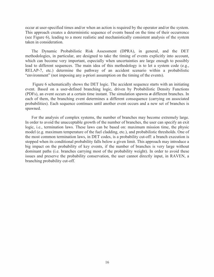
occur at user-specified times and/or when an action is required by the operator and/or the system.This approach creates a deterministic sequence of events based on the time of their occurrence (see Figure 6), leading to a more realistic and mechanistically consistent analysis of the system taken in consideration.

The Dynamic Probabilistic Risk Assessment (DPRA), in general, and the DET methodologies, in particular, are designed to take the timing of events explicitly into account, which can become very important, especially when uncertainties are large enough to possibly lead to different sequences. The main idea of this methodology is to let a system code (e.g., RELAP-7, etc.) determine the pathway of an accident scenario within a probabilistic “environment” (not imposing any a-priori assumption on the timing of the events).

Figure 6 schematically shows the DET logic. The accident sequence starts with an initiating event. Based on a user-defined branching logic, driven by Probabilistic Density Functions (PDFs), an event occurs at a certain time instant. The simulation spawns n different branches. In each of them, the branching event determines a different consequence (carrying on associated probabilities). Each sequence continues until another event occurs and a new set of branches is spawned.

For the analysis of complex systems, the number of branches may become extremely large.In order to avoid the unacceptable growth of the number of branches, the user can specify an exit logic, i.e., termination laws. These laws can be based on: maximum mission time, the physic model (e.g. maximum temperature of the fuel cladding, etc.), and probabilistic thresholds. One of the most common termination laws, in DET codes, is a probability cut-off: a branch execution is stopped when its conditional probability falls below a given limit. This approach may introduce a big impact on the probability of key events, if the number of branches is very large without dominant paths (i.e. branches carrying most of the probability weight). In order to avoid these issues and preserve the probability conservation, the user cannot directly input, in RAVEN, abranching probability cut-off.

17

5. THE HYBRID DYNAMIC EVENT TREE METHOD

In the UQ field, the uncertainties are generally grouped into two main types:

Aleatory uncertainties: uncertainties caused by an intrinsic variation or randomness.Aleatory uncertainties are generally characterized by a probability distribution, most commonly as either a probability density function (PDF) – which quantifies the probability density at any value over the range of the random variable – or a cumulative distribution function (CDF) – which quantifies the probability that a random variable will be less than or equal to a certain value;

Epistemic uncertainties: uncertainties caused by to a lack of knowledge that the analysts,conducting the modeling and simulation, have. If knowledge is added (through experiments, improved numerical approximations, expert opinion, higher fidelity physics modeling, etc.) then the uncertainty can be reduced. If sufficient knowledge is added, then the epistemic uncertainty can, theoretically, be eliminated. Epistemic uncertaintiesare traditionally represented as an interval of variability with or without associated aprobability density function. In contrast to aleatory uncertainties, the probability density function, if present, represents degree of belief of the analysts, instead of frequency of occurrence. A typical parameter affected by epistemic uncertainty, in the modeling of the thermal-hydraulic systems, is the friction factor of the piping system, which is generally dependent on the flow regime and computed through empirical correlations.

The treatment of such aleatory uncertainties is quite challenging from a modeling point of view, since it requires an internal random sampling scheme directly implemented in the system simulator or a methodology that can “evolve” its exploration strategy based on the dynamic of the system. On the other side, the exploration of the epistemic uncertainties is generally performed through Monte-Carlo or Latin Hyper Cube methods, that can be computational expensive.

In order to overcome the computational burden of these methods and to correctly model aleatory uncertainties, the Dynamic Event Tree approach has been developed. The DET methodologies are particularly indicated to treat uncertainties that lead to state transitions of the analyzed system. In other words, events characterized by a time and a system state change, each of which may be either deterministic or aleatory and discrete, can be treated by the DET methods.

18

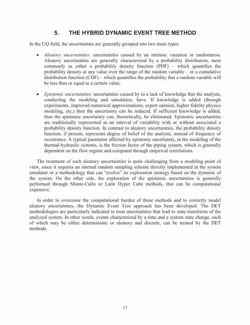
Figure 7 - Epistemic uncertainties’ treatment with basic Dynamic Event Tree method.

The DET method is particularly indicated for the treatment of the aleatory uncertainties, since they can represent events that might happen during an accident/transient scenario and not characterizing the initial condition. On the other hand, the epistemic uncertainties systematically affect all the calculations, being translated in bias of the parameters used in the modeling of the system.

From a DET point of view, the epistemic uncertainties can be treated, by the basic DET approach by employing a multi-branch feature. As shown in Figure 7, at the begin of the simulation (i.e., time = 0.0), the DET triggers multiple branches, one branch for each user-specified vector eu of the epistemic uncertainties. From each branch, a standard DET (see Section 4) begins. Hence, the DET methodology already let the user treat the epistemic uncertainties using the already capabilities available in RAVEN. Obviously, this approach can become cumbersome when a large number of epistemic uncertainties need to be taken in account: the method needs to be automatized.

In order to make the DET capable to automatically handle these types of uncertainties, it is needed to extend the DET approach by embedding forward sampling strategies (e.g., Monte-Carlo, etc.). This upgrade has been named, by the authors, “Hybrid Dynamic Event Tree” (HDET) method.

The HDET method represents an evolution of similar methodologies (e.g., MCDET [20]) for the simultaneous exploration of both epistemic and aleatory uncertainties. In these methods the uncertainties are generally treated employing a Monte-Carlo sampling approach (epistemic) and

19

DET methodology (aleatory). The HDET methodology developed within the RAVEN code can also use additional sampling strategies. The epistemic or epistemic-like uncertainties can be sampled through the following strategies:

Monte-Carlo;

Grid sampling;

Stratified (e.g., Latin Hyper Cube).

Figure 8 schematically shows how the HDET methodology works. The user defines the parameters that need to be sampled by one or more different forward sampling approaches. The HDET module samples (e.g., Monte Carlo, Grid, Stratified, etc.) those parameters (epistemic uncertainties) by creating a N-Dimensional set of points. Each point in the input space represents a starting point for a separated standard Dynamic Event Tree exploration of the uncertain domain.

The HDET methodology allows the user to completely explore the uncertain domain employing one methodology. The addition of Grid sampling strategy among the approaches usable, allow the user to perform a discrete parametric study, under both aleatory and epistemic uncertainties.

Figure 8 – Hybrid Dynamic Event Tree conceptual scheme

20

6. THE ADAPTIVE HYBRID DYNAMIC EVENT TREE

As shown in the previous section, the HDET and the DET approaches are extremely effective (achieving almost a perfect tradeoff) with respect to the computational resources usage and the effective exploration of the uncertain domain (input space).

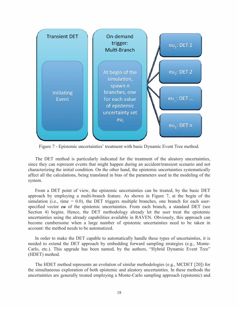
As shown in [9,10], the RAVEN code already posses an adaptive methodology based on the DET approach (ADET). This approach is designed to exploit the DET methodology in order tocharacterize some properties of the uncertain space. More specifically, the ADET approach is an adaptive methodology that automatically guides the branching strategy in order to identify more efficiently (lower computational costs) and more accurately the location of transitions in the input space (e.g., failure vs. success). The characterization of the input space is translated into an optimization-like problem for the identification of the so-called Limit Surface, and accelerated through the employment of artificial intelligence-based algorithms (Reduced Order Models, ROMs) that help the selection of forthcoming branching conditions.

In order to explain how the already-present ADET methodology has been evolved into the Adaptive Hybrid Dynamic Event Tree (AHDET), it is important to briefly review the concept of Limit Surface (section 6.1), ROM (section 6.2) and the current ADET implementation (section 6.3). The newly developed AHDET method is, then, explained in section 6.4.

6.1 Limit Surface

The adaptive methodology can be considered a goal-oriented sampling strategy for the research of the Limit Surfaces (LSs). To define the meaning of the LS, it is necessary to introduce the concept of “goal” function. The “goal” function is an object that is defined as a part of the system outcome space. In a safety context, the goal function usually represents the success or failure (transition) of the system.

If is the status of the system and ( ) the goal function ( ( ) = : system success, ( ) = : system failure), it is possible to define , as the transition surface in the output space with respect to the goal function. This statement can be translated in the following mathematical expression: , = { | = }.

If ( , , ) represents the evolution of the system, then is it possible to identify the set of pairs ( , ) , in the input space, which leads the system outcome to match , . Such set of points in ( , ) represents the limit surface, in the input space. The LS represent therefore the boundary between inputs leading to success or failure of the system, and more generally boundaries among transition regions.

Since the probability of a particular outcome is equivalent to the probability of the combination of uncertainties that led to such outcome, the computation of the weighted integral of the LS corresponds to the probability of the event (e.g. failure/success) modeled by the goal function.

The determination of the LS is important because of its informative content:

21

1) It allows to efficiently evaluate risk functions

2) It determines which uncertainties are the most relevant from a risk point of view

3) It defines safe regions to be explored for plant optimization, 4) identifies risk neutral design direction, etc.

As better explained in section 6.3, the LS search algorithm requires the discretization of the uncertain domain, constructing a N-Dimensional grid. This discretization is done such that the probability content of each cell is proportional to a user-defined tolerance. In order to locate the LS, one would need to run a number of calculations equal to the number of nodes in the grid. Obviously, this approach, in most of the cases, is not feasible (i.e. too computational expensive).

In order to overcome these limitations, it is possible to employ acceleration schemes based on Reduced Order Models (ROMs). ROMs are used to predict the location of the LS and to iteratively guide the exploration of the input space. Both ADET and AHDET are based on this concept.

6.2 Reduced Order Models

As mentioned in the previous section, ADET and AHDET use ROMs in order to accelerate the search of the LS. Simplistically, a ROM is a mathematical model of fast solution trained to predict a response of interest of a physical system. The training process is performed by “sampling” the response of a physical model with respect to variations of parameters that are subject to probabilistic behavior. These samples are fed into the ROM that tunes itself to replicate those results.

In the RAVEN case the ROM is constructed to emulate a numerical representation of a physical system. In fact, as already mentioned, the physical system model would be too expensive to be used to explore the whole input space, exploration that would be needed for theLS identification.

In RAVEN, several ROMs are available: Support Vector Machine, Neighbors based, multi-class models, Quadratic Discriminants, etc. All these ROM have been imported via an Application Programming Interface (API) within the scikit-learn library [21] and few have been also specifically developed (e.g. Polynomial Chaos, N-Dimensional Spline regressors, etc.).

The acceleration schemes in the adaptive approach use a class of ROMs usually referred to as “classifiers.” In essence, classifiers are ROMs specialized to represent a binary response of a system (e.g., failure/success, on/off, etc.), like the goal function of interest in our case.

22

Figure 9 - A-posteriori Limit Surface generated from standard DET

6.3 Adaptive Dynamic Event Tree

The main idea behind the application of adaptive sampling techniques to the DET comes from the observation that the DET is intrinsically adaptive.

In order to explain this statement Figure 9 shows an example of LS generated by the DET sampling methodology currently available in RAVEN. In this case, a goal function based on the clad max temperature has been used:

{ } = 1 , ,1 , < , (1)

where , is the clad temperature and , is the failure temperature, sampled by triangular distribution.

As it can be seen in Figure 9, the DET method tends to search for the LS with accuracy equal to the user-defined grid discretization in the N-dimensional space of the aleatory variables. For this reason, it appeared natural to use the DET approach to perform a goal-function oriented pre-sampling (usually referred as initial training set) of the input space.

The proposed approach can be described through the following steps (see Figure 10):

1. A limited number of points in the aleatory space ( , ) are selected via a DET approach;

2. The system code is used to compute all the possible evolution of the system starting the above selected input points:

23

( ) = , , , (2)

3. The goal function (in this case, Boolean) is evaluated at the end of the simulation:{ } = { = , , , } (3)

4. The set of pairs {( , ) , { } } are used to train a ROM;

5. The ROM is used to predict the value of the goal function on a regular Cartesian grid in the input space. The grid meshing is dictated by the user-requested accuracy in the determination of the LS location: { } { } , = 1, … , (4)

where j=1,…,M points on the grid

6. The points where a change in the value of { } occurs are the ROM prediction of the limit surface location ( , ) ;

7. The position of the LS is compared with the one at the previous iteration; if no changes are consecutively detected for a user-defined number of times than the iterations stop; otherwise a new point in the input space is selected to increase the ROM training set;

8. The next selected point to be added to the training set is the one located on the limit surface that is the farther from all the other already selected points;

9. A hierarchical searching process is performed on the DET branches already evaluated and the starting point (branch) for the new evaluation is determined;

10. The process restarts from point 2.

24

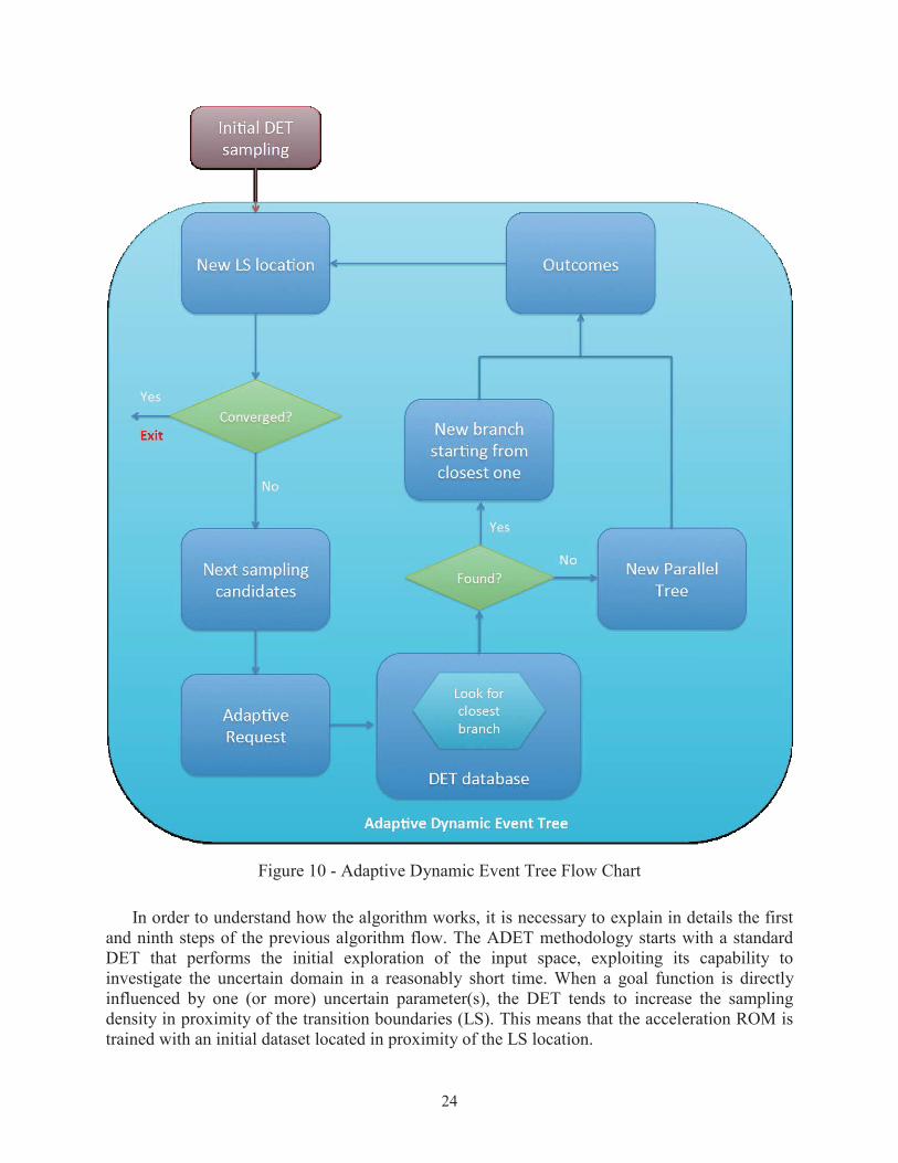
Figure 10 - Adaptive Dynamic Event Tree Flow Chart

In order to understand how the algorithm works, it is necessary to explain in details the first and ninth steps of the previous algorithm flow. The ADET methodology starts with a standard DET that performs the initial exploration of the input space, exploiting its capability to investigate the uncertain domain in a reasonably short time. When a goal function is directly influenced by one (or more) uncertain parameter(s), the DET tends to increase the sampling density in proximity of the transition boundaries (LS). This means that the acceleration ROM istrained with an initial dataset located in proximity of the LS location.

25

When the initial DET is completed, the actual adaptive scheme is employed by following the calculation flow previously reported. Every time a new point, in the input space, is requested, a search in the DET database is performed. This search is needed to identify the closest branch with respect to the next point needs to be evaluated.

The concept of closest branch is more extensively explained in [9], for the purpose of this report it is sufficient to say that it is a branch that has the probability of developing into the state sought and computationally speaking is the one that would allow reaching the sought branching condition with the minimal simulation cost. Once the closest branch has been identified, the system code is run using that branch as starting point (i.e. the calculation restarts from an advanced point in time). This new evaluation is then added to the DET database and can be used for sub-sequential requests. This approach speeds up the adaptive search up and employs an effective exploration of the input space in proximity of the transition boundaries.

In essence this methodology combines the LS search algorithm with a DET approach, allowing the re-usage of branches of simulations already performed rather than restarting the simulation always from the begin of the scenario under consideration.

6.4 Adaptive Hybrid Dynamic Event Tree methodology

As reported in Section 5, the HDET represents an evolution of the DET method for the simultaneous exploration of the aleatory and epistemic space. In addition, it has reported how the Adaptive DET methodology, developed during last Fiscal Year [9], is implemented in RAVEN. An additional effort has been performed this year in order to upgrade the HDET in order to drive an Adaptive Limit Surface search process. The authors have named the new method Adaptive Hybrid Dynamic Event Tree (AHDET).

The main idea of the AHDET method is to extend the ADET method in order to consider,the epistemic uncertainties in the LS search. Two different options have been designed/developed in order to accomplish this task:

1) The epistemic uncertainties are not actively part of the Limit Surface search (they are not part of the search domain);

2) The epistemic uncertainties are active part of the LS search process.

In the following sub-sections both options are explained.

26

Figure 11 - AHDET: Epistemic uncertainties not projected in the LS space.

6.4.1 AHDET: Epistemic uncertainties not projected in the LS space

The first available option in the AHDET method is based on the assumption that some epistemic (more precisely, epistemic-like) uncertainties do not need to be projected in the LimitSurface space (complete uncertain domain). This can happen when the analysis of a dynamic scenario, affected by aleatory uncertainties, is needed to be performed in conjunction with a parametric study; for example, a Station Black Out scenario analysis as function of the power uprate (epistemic-like uncertainty is, then, the power level).

For such cases, the Adaptive Hybrid Dynamic Event Tree is employed following a calculation scheme as follows (see Figure 11):

1) The AHDET module samples the epistemic uncertainties (user-defined parameters) based on one or more different forward sampling approaches;

2) An N-Dimensional grid, characterized by all the possible combinations of the epistemic space coordinates coming from the different sampling strategies, is generated;

3) Each coordinate in the epistemic space is associated to a Adaptive DET process;

4) When all the Adaptive DET processes end (see Section 6.3), a converged LS is obtained: one for each coordinate in the epistemic space (for an hypothetical example,see Figure 12).

Optionally, the user can request the convolution of the LSs in order to obtain a single hyper surface in the complete (epistemic and aleatory) uncertain space.

27

Figure 12 – Example of LSs at different levels of an epistemic uncertain parameter.

Figure 13 - AHDET: Epistemic uncertainties active part of the LS search process.

6.4.2 AHDET: Epistemic uncertainties projected in the LS space.

The second available option in the AHDET module is based on the consideration that the epistemic uncertainties are actively part of the LS search process. They are considered as additional features characterizing the N-Dimensional LS. If the final goal of the analysis is the computation of the probability of certain final events (e.g. probability of core melting in Reactor Safety analyses), then this is the preferable approach since all the uncertain parameters (aleatory and epistemic) are considered in the same complete domain. An example of this approach is the

28

search of the safest point where the input space posses both the variables subject to parametric analysis and uncertainty [22].

For such cases, the Adaptive Hybrid Dynamic Event Tree is employed by following thiscalculation scheme (see Figure 13):

1) The AHDET module generates an evaluation N-Dimensional grid, based on the user-defined LS convergence criterion (tolerance in probability). The number of dimensions of the grid equals the number of uncertainties under consideration (epistemic and aleatory). The discretization step size in each dimension is built such the volume of each N-Dimensional cell is proportional to the user-defined tolerance;

2) The discretization coordinates of each epistemic variable are then used to build an additional N-Dimensional grid, characterized by all the possible combinations of the epistemic space coordinates;

3) The AHDET starts the LS search, considering the epistemic N-Dimensional grid as part of the searching domain.

4) Every time a new point to investigate is requested, the AHDET searches for the corresponding tree characterized by the requested coordinate in the epistemic space and an ADET process is employed;

5) The process at 4) is repeated until the LS converges.

At end of this process, the converged LS is shown to the user.

29

7. PROOF OF CONCEPT: PRA ANALYSIS ON A SIMPLIFIED PWR-LIKE MODEL

In order to demonstrate the potential of the newly developed HDET and AHDET, a PRA analysis of a Station Black Out (SBO) on a simplified PWR-like has been performed (using RELAP-7). In the following sections, some representative results are reported for both methodologies.

7.1 PWR system.

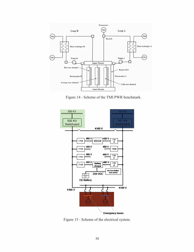
A PWR simplified model has been set up based on the parameters specified in the OECD main steam line break (MSLB) benchmark problem [23]. The reference design for the OECD MSLB benchmark problem is derived from the reactor geometry and operational data of the TMI-1 Nuclear Power Plant (NPP), which is a 2772 MW two loop pressurized water reactor (see the system scheme shown in Figure 14).

In order to simulate a SBO initiating event, the following electrical systems have been considered (see Figure 15):

Primary and auxiliary power grid lines (500 KV and 161 KV) connected to the respectively switchyards;

Set of 2 diesel generators (DGs), DG1 and DG2, and associated emergency buses;

Electrical buses: 4160 V (step down voltage from the power grid and voltage of the electric converter connected to the DGs) and 480 V for actual reactor components (e.g., reactor cooling system)

DC system, which provides power to instrumentation and control components of the plant. It consists of these two sub-systems: battery charger and AC/DC converter and DC batteries.

30

Figure 14 - Scheme of the TMI PWR benchmark.

Figure 15 - Scheme of the electrical system.

31

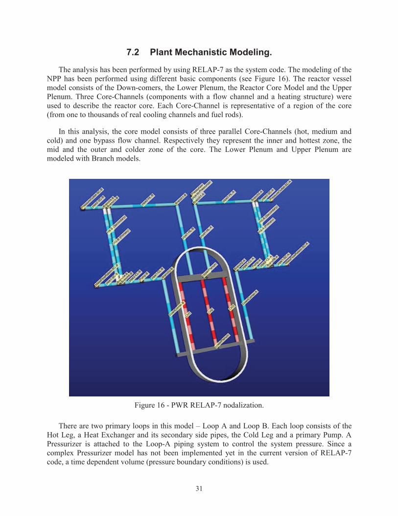
7.2 Plant Mechanistic Modeling.

The analysis has been performed by using RELAP-7 as the system code. The modeling of the NPP has been performed using different basic components (see Figure 16). The reactor vessel model consists of the Down-comers, the Lower Plenum, the Reactor Core Model and the Upper Plenum. Three Core-Channels (components with a flow channel and a heating structure) were used to describe the reactor core. Each Core-Channel is representative of a region of the core (from one to thousands of real cooling channels and fuel rods).

In this analysis, the core model consists of three parallel Core-Channels (hot, medium and cold) and one bypass flow channel. Respectively they represent the inner and hottest zone, the mid and the outer and colder zone of the core. The Lower Plenum and Upper Plenum are modeled with Branch models.

Figure 16 - PWR RELAP-7 nodalization.

There are two primary loops in this model – Loop A and Loop B. Each loop consists of the Hot Leg, a Heat Exchanger and its secondary side pipes, the Cold Leg and a primary Pump. A Pressurizer is attached to the Loop-A piping system to control the system pressure. Since a complex Pressurizer model has not been implemented yet in the current version of RELAP-7code, a time dependent volume (pressure boundary conditions) is used.

32

7.3 SBO Scenario.

The scenario considered is a loss of off-site power (LOOP) initiating event caused by an earthquake (in proximity of the NPP), followed by tsunami induced flooding. The wave height is such that it causes water to enter into the air intake of the DGs and temporary disable the DGs themselves. In more detail, the scenario is the following:

1. An external event (i.e., earthquake) causes a LOOP due to damage of both 500 kV and 161 kV lines; the reactor successfully scrams and, thus, the power generated in the core follows the characteristic exponential decay curve;

2. A tsunami wave hits the plant causing flooding of the plant itself. The wave causes the DGs to fail and may also flood the 161 kV switchyard. Hence, conditions of SBO are reached (4160 V and 480 V buses are not energized); all core cooling systems are subsequently off-line (including the ECCS system);

3. Without the ability to cool the reactor core, its temperature starts to rise;

4. In order to recover AC electric power on the 4160 V and 480 V buses, three strategies are followed:

A plant recovery team is assembled in order to recover one of the two DGs;

The power grid owning company is working on the restoration of the primary 161kV line;

A second plant recovery team is also assembled to recover the 161 kV switchyard if flooded.

5. When the 4160 kV buses are energized (through the recovery of the DGs or 161 kV line), the auxiliary cooling system (i.e., ECCS system) is able to cool the reactor core and, thus, core temperature decreases.

7.4 Aleatory uncertainties.

In this scenario, the cooling of the reactor (through the ECCS system) is ensured when either the DGs or the 161 kV line are restored. Since the purpose of this report is to demonstrate the potential of the HDET and AHDET methodologies in the RAVEN code, both the DGs and the 161 kV line recovery times are collapsed in one single stochastic parameter (tECCS).

The failure of the plant occurs when the cladding in the core reaches its failure temperature. The clad failure temperature value (Tfailure) is considered stochastic as well.

33

7.5 Epistemic uncertainties.

In this section, the epistemic uncertainties considered in the SBO analysis using the HDET and AHDET methodologies are reported. As it can be inferred from the following sub-sections, two different sets of epistemic uncertainties have been considered.

7.5.1 Epistemic uncertainties used in HDET sampling strategy

In order to show the HDET capabilities and its way to treat epistemic or “epistemic-like” uncertainties by the combination of its main sampling strategies (i.e. Monte-Carlo, Stratified and Grid samplers), 3 different epistemic or “epistemic-like” parameters have been considered.

One of the most common epistemic uncertainties taken in account in such analysis are the friction factors of the piping network. As proof of concept, in the demo case presented here,uncertainties in the friction factors of the three core channels have been considered.

Another important source of uncertainties, in this kind of scenarios, is represented by the “accuracy” of the model used to simulate, right after the “scram” of the reactor, the decay heat generation. If it is not computed by appropriated Burn-Up codes [24], its evolution, right after the scram, is generally modeled by user-input approximated exponential decay curves (Decay Power vs. time). In RELAP-7 (i.e., in its module CROW [3]), a set of predefined curves is already available. For this analysis, a curve characterized by the following equation has been employed: ( ) = ( + + . ) . + + . . .( + + ) . ( + + + ) . (5)

where, P0 is the initial power, is the power coefficient (% of decay power with respect to the nominal power), tstart is the scram time, top is the time the NPP has been at P0 power level. In order to investigate the effects of the approximations in this modeling strategy, the power coefficient has been considered as an epistemic uncertainty.

Finally, the third parameter that has been considered is one that can be included among the so-called “epistemic-like” uncertain factors: the operational power. Even if it is not a real epistemic uncertainty, it is interesting to investigate, in a parametric fashion, the effects of perturbations on the operational power level.

7.5.2 Epistemic uncertainties used in AHDET sampling strategy

In order to show the AHDET capabilities and the resulting LS search algorithm, the following epistemic and “epistemic-like” uncertainties have been considered:

34

Friction factor coefficients (fscaling) of the three core-channels representing the Thermal-Hydraulic of the whole core. The uncertainties associated to these friction factors have been modeled through a scaling factor;

Power uprate level (Pscaling), treated as a multiplicative factor of the operational power.

As it can be inferred, the number of epistemic uncertainties has been reduced with respect the one considered for the HDET showcase. This has been done for visualization purposes only; indeed, considering 2 epistemic uncertainties, in conjunction with the 2 aleatory ones, allowed to still visualize the resulting LS in a 3-Dimensional scatter plot (4th dimension is visualized through a color map of the scattered points).

7.6 Stochastic model.

As in any PRA process, the uncertainties under consideration are modeled through the definition of associated PDFs. In the following two subsections, the stochastic model for each of the uncertainty previously mentioned is reported.

7.6.1 Stochastic model: Aleatory uncertainties.

Regarding the parameters affected by aleatory uncertainties, the following PDFs have been used:

ECCS recovery time (tECCS):

o Normal distribution,

Mean: 3125 seconds

Sigma: 850 seconds

Clad Failure Temperature (Tfailure):

o Triangular distribution,

Peak: 1477.59 K

Lower: 1255.37 K

Upper: 1699.81 K

The recovery of the ECCS system has been considered being “faster” than the reality (mean ~hours) since the transient timing has been shrunk.

35

The effects of both aleatory parameters have been explored, by the DET part of the HDETand AHDET methods, using a grid in CDF characterized by the following thresholds: 0.01, 0.1, 0.2, 0.3, 0.4, 0.5, 0.6, 0.7, 0.8, 0.85, 0.9, 0.95. This means that a branch occurs when either the clad temperature or the time corresponds to a CDF equal or bigger than the probability threshold imposed by the sampler.

7.6.2 Stochastic model: Epistemic uncertainties.

As stated in Section 7.5, the number of uncertainties considered in the showcases for the HDET and AHDET methodologies is different. In the following subsections, the stochastic model for each of them is reported.

7.6.2.1 Stochastic model: Epistemic uncertainties in HDET showcase.

Regarding the parameters affected by epistemic uncertainty, for the HDET showcase, the following probability density functions have been used:

Friction scaling factor (fscaling):

o Truncated Normal distribution,Mean: 1.0 (-)

Sigma: 0.2 (-)

Lower: 0.5 (-)

Upper: 1.5 (-)

Decay heat curve power coefficient ( scaling):

o Truncated Normal distribution,Mean: 1.0 (-)

Sigma: 0.2 (-)

Lower: 0.5 (-)

Upper: 1.5 (-)

Power scaling factors (Pscaling):

o Uniform distribution,

Lower: 1.0 (-)

Upper: 1.2 (-)

As can be inferred from above, the same “sampled” multiplier fscaling scales the friction factors of the three core channels.

36

The parameters above have been perturbed through the following strategies (Table 4):

Table 4 - Epistemic Sampling settings

Parameter Sampler Grid Size # samples or nodesfscaling Grid 0.33 [CDF] 4scaling MonteCarlo - 4Pscaling Stratifieda 0.33 CDF 4

This approach led to a 3-Dimensional grid of 64 combinations and, thus, 64 parallel DET simulations spawned.

7.6.2.2 Stochastic model: Epistemic uncertainties in AHDET showcase

Regarding the parameters affected by epistemic uncertainty, for the AHDET showcase, the following probability density functions have been used:

- Friction scaling factor (fscaling):

o Truncated Normal distribution,Mean: 1.0 (-)

Sigma: 0.2 (-)

Lower: 0.5 (-)

Upper: 1.5 (-)

- Power scaling factors (Pscaling):

o Uniform distribution,Lower: 1.0 (-)

Upper: 1.2 (-)

As for the HDET showcase, the same “sampled” multiplier fscaling scales the friction factors of the three core channels.

7.7 Results

In this section the results for both methodologies applied to the SBO scenario are reported. Firstly, the results obtained with the HDET methodology are going to be analyzed and discussed; consequentially, the AHDET ones.

a For demonstration purposes the Stratified sampling strategy has been employed with a single variable; for this reason, it practically consists of a grid sampling with random bin size.

37

7.7.1 SBO scenario analyzed through HDET methodology

The HDET analysis has been performed and about ~2,100 branches were obtained; these resulted in ~1,600 completed histories.

Figure 17 shows the clad temperature temporal evolution for all the histories generated by the HDET. The different colors represent the distinctive branches that have been simulated. It can be noticed that the temperature starts raising right after the initiating event and the raising paths are slightly diverging (the slope coefficients change). This behavior is connected to the sampling of the initial power level and decay curve coefficient.

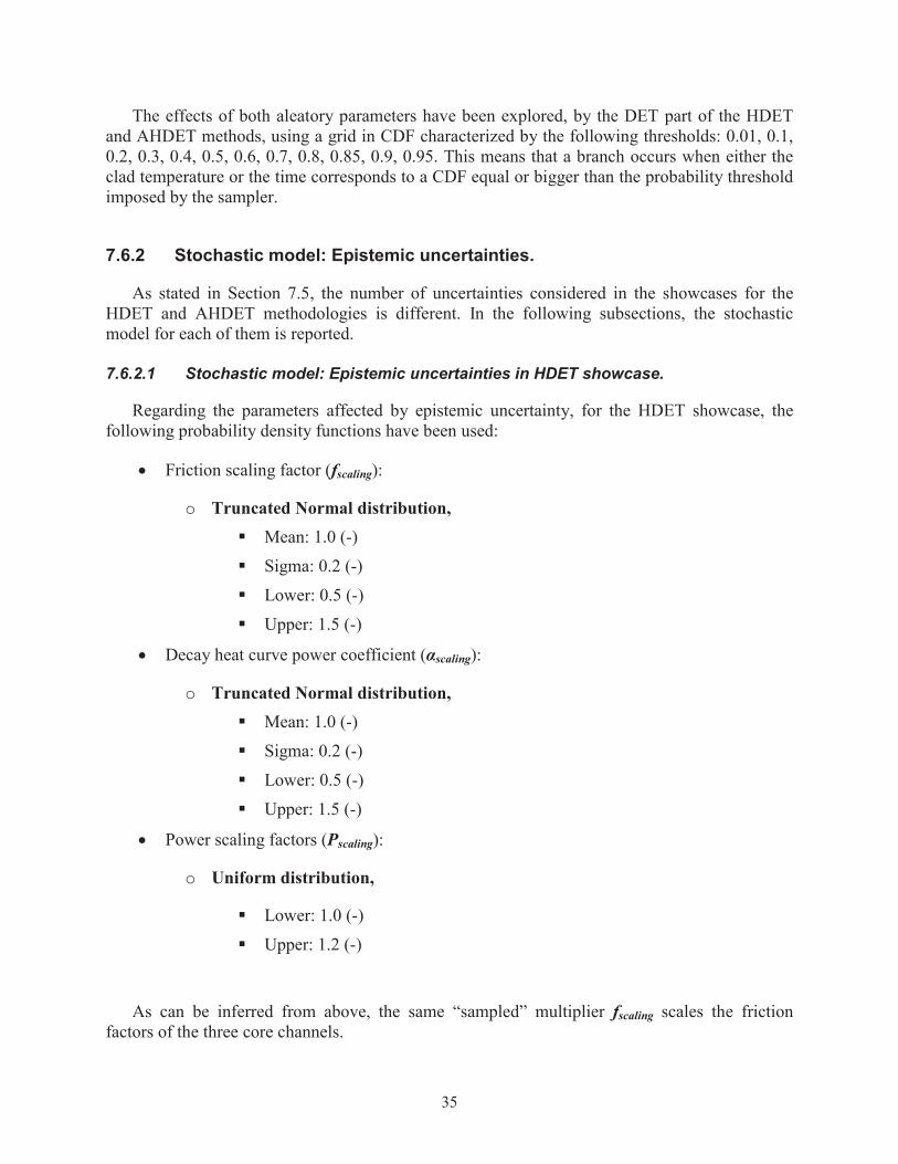
Figure 18 shows the flow velocity evolution in the cold leg. It can be noticed the velocity oscillations right after the back up of the ECCS system. These oscillations are determined since the sudden insertion of the system. Indeed, for this analysis, the ECCS action has been modeled by setting the pumps’ head to 5% of the nominal one, with a very fast ramp-up.

Figure 17 - HDET clad temperature evolution.

38

Figure 18 - HDET cold leg flow velocity evolution.

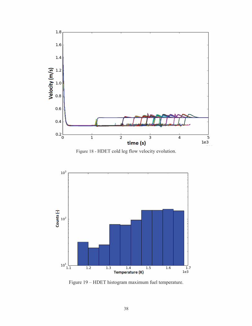
Figure 19 – HDET histogram maximum fuel temperature.

39

Figure 20 – HDET histogram maximum clad temperature.

Figure 19 and Figure 20 show the histograms of the fuel and clad maximum temperatures,respectively. It can be noticed that the most populated bins are those at higher temperatures, since, the clad failure temperature is a stochastic parameter, that is translated into a forward movement of the clad failure temperature threshold. For this case, the probability of failure of this system is 9.33E-04.

7.7.2 SBO scenario analyzed through AHDET methodology.

As mentioned in Section 6, the convergence of the AHDET method is based on the construction of an evaluation N-Dimensional grid, whose discretization is driven by a user-defined tolerance value and a weight metric (CDF or absolute value). The discretization of the Cartesian grid is made such that each cell volume is proportional to the inputted tolerance depending on the user-inputted weight metric:

If the weight is in CDF, each cell has a probability content equal to the tolerance;

If the weight is in absolute value, each cell has a volume equal to the total volume (hyper-volume of the full uncertain domain) multiplied by the tolerance.

In order to show the newly developed methodology, the tolerance has been set to 1.e-4 in CDF (weight).

40

Figure 21 - Clad Temperature evolution for Core Channel 1 and 2.

For the scope of this report, only the results for the AHDET option in which the epistemic uncertainties are part of the LS search process are reported. The AHDET analysis has been performed, obtaining ~1200 branches resulting in ~630 completed histories.

Figure 21 shows the clad temperature temporal evolution for all the histories generated by the AHDET. As for the HDET, the different colors represent the distinctive branches that have been simulated. It can be noticed that the temperature starts raising right after the initiating event and the raising paths are slightly diverging (the slope coefficients change). This behavior is connected to the sampling of the initial power level. In addition, it can be noticed that the plots present a higher density of branches in the ascending portions of the histories; this is because the AHDET focalizes the computational effort along the Limit Surface, investigating the combination of events that leads to the failure of the system.

Figure 22 - Pump Head evolution.

41

Figure 22 shows the pump head evolution. In this figure, the ECCS quick rump-up can be seen. As already mentioned, this approach determines the oscillation in the water velocity shown in previous section.

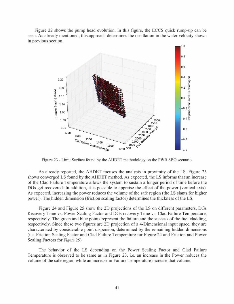
Figure 23 - Limit Surface found by the AHDET methodology on the PWR SBO scenario.

As already reported, the AHDET focuses the analysis in proximity of the LS. Figure 23shows converged LS found by the AHDET method. As expected, the LS informs that an increase of the Clad Failure Temperature allows the system to sustain a longer period of time before the DGs get recovered. In addition, it is possible to appraise the effect of the power (vertical axis). As expected, increasing the power reduces the volume of the safe region (the LS slants for higher power). The hidden dimension (friction scaling factor) determines the thickness of the LS.

Figure 24 and Figure 25 show the 2D projections of the LS on different parameters, DGs Recovery Time vs. Power Scaling Factor and DGs recovery Time vs. Clad Failure Temperature, respectively. The green and blue points represent the failure and the success of the fuel cladding, respectively. Since these two figures are 2D projection of a 4-Dimensional input space, they are characterized by considerable point dispersion, determined by the remaining hidden dimensions (i.e. Friction Scaling Factor and Clad Failure Temperature for Figure 24 and Friction and Power Scaling Factors for Figure 25).

The behavior of the LS depending on the Power Scaling Factor and Clad Failure Temperature is observed to be same as in Figure 23, i.e. an increase in the Power reduces the volume of the safe region while an increase in Failure Temperature increase that volume.

42

Figure 24 - Limit Surface 2D projection: Combined effect of Power and DGs recovery time.

Figure 25 - Limit Surface 2D projection: Combined effect of Failure Temperature and DGs recovery time.

43

8. CONCLUSIONS

This report presented two distinct development features that have been accomplished during FY 2015. The migration of the RAVEN/RELAP-7 control logic system into the MOOSE framework has begun and an initial set of capabilities have been shown. The migration of the control logic system directly into the MOOSE framework opens interesting possibilities for the future. The system is going to let the RAVEN code to drive, through all its dynamic advanced methodologies (i.e. Dynamic Event Tree based sampling strategies, etc.), any MOOSE-based application, that it is designed to be used for dynamic scenario analysis. This feature is likely going to be finalized in FY 2016.

The second development that has been here presented is the Hybrid Dynamic Event Tree and its variant, the Adaptive Hybrid Dynamic Event Tree. The addition of these methods improves the capability of the Dynamic Event Tree to:

Explore the uncertain domain, under epistemic uncertainties and for parametric studies;

Consistently reduce the computational time and improve the convergence for the search of the Limit Surface and, consequentially, for the determination of the failure probability of a certain system (e.g. NPP).

The methodology concepts and all the main components that are involved in the computation have been described, including the used system simulator (e.g., RELAP-7). A proof of concept of a PRA analysis has been also shown for a SBO scenario for a simplified PWR loop. The description of the implementation for such case demonstrates how the flexibility of the software framework provides advanced tools to perform Dynamic PRA, uncertainty quantification and plant control.

The HDET and AHDET methodologies are part of a development around the concept of DET and goal-oriented exploration of the uncertain domain [7,8,9,10,25]. The implementation of these methodologies determines the basis for a future class of algorithms, under development by the authors, which are designed to exploit the intrinsic characteristics of DET-based methods.

44

REFERENCES

[1] A. Alfonsi, C. Rabiti, D. Mandelli, J. Cogliati, and R. Kinoshita, “Raven as a tool for dynamic probabilistic risk assessment: Software overview,” in Proceeding of M&C2013 International Conference on Mathematics and Computational Methods Applied to Nuclear Science & Engineering, on CD-ROM, May 5-9, Sun Valley (2013).

[2] C. Rabiti, A. Alfonsi, D. Mandelli, J. Cogliati, R. Martinueau, C. Smith, “Deployment and Overview of RAVEN Capabilities for a Probabilistic Risk Assessment Demo for a PWR Station Blackout,” Idaho National Laboratory report: INL/EXT-13-29510 (2013).

[3] A. Alfonsi, C. Rabiti, D. Mandelli, J. Cogliati, R. Kinoshita, and A. Naviglio, “RAVEN and dynamic probabilistic risk assessment: Software overview,” in Proceedings of ESREL European Safety and Reliability Conference, Wroclaw, Poland (2014).

[4] A. Alfonsi, C. Rabiti, D. Mandelli, J. Cogliati, R. Kinoshita, “Performing Probabilistic Risk Assessment Through RAVEN”, in Proceedings of American Nuclear Society 2013 Annual Meeting “Next Generation Nuclear Energy: Prospects and Challenges”, Atlanta, GA (2013).

[5] C. Smith, C. Rabiti, and R. Martineau, “Risk Informed Safety Margins Characterization (RISMC) Pathway Technical Program Plan”, Idaho National Laboratory INL/EXT-11-22977 (2011).

[6] David, R. Berry, D. Gaston, R. Martineau, J. Peterson, H. Zhang, H. Zhao, L. Zou, “RELAP-7Level 2 Milestone Report: Demonstration of a Steady State Single Phase PWR Simulation with RELAP-7,” Idaho National Laboratory: INL/EXT-12-25924 (2012).

[7] A. Alfonsi, C. Rabiti, D. Mandelli, J. Cogliati, R. Kinoshita, A. Naviglio, “Dynamic Event Tree Analysis Through RAVEN”, in Proceedings of International Topical Meeting on Probabilistic Safety Assessment and Analysis (PSA 2013), September 22-26, Columbia, SC, USA, (2013).

[8] A. Alfonsi, C. Rabiti, D. Mandelli, J. Cogliati, R. Kinoshita, “RAVEN: Dynamic Event Tree Approach. Level III Milestone”, Idaho National Laboratory, Idaho Falls, Idaho, INL/EXT-13-30332, (2013).

[9] A. Alfonsi, C. Rabiti, D. Mandelli, J. Cogliati, and R. Kinoshita, “RAVEN: Development of the adaptive dynamic event tree approach,” Tech. Rep. INL/MIS-14-33246, Idaho National Laboratory (INL), (2014).

[10] A. Alfonsi, C. Rabiti, D. Mandelli, J. Cogliati, and R. Kinoshita, “Adaptive Dynamic Event Tree in RAVEN code,” in Proceedings of American Nuclear Society 2014 Winter Meeting “Nuclear-The Foundation of Clean Energy”, Anaheim, CA (2014).

[11] P. C. Cacciabue, A. Amendola, G. Cojazzi, “Dynamic Logical Analytical Methodology Versus Fault Tree: The Case Study of the Auxiliary Feedwater System of a Nuclear Power Plant”, Journal of Nuclear Technology, Volume 74, Number 2, pp 195-208, (1986).

[12] D. Gaston, C. Newman, G. Hansen and D. Lebrun-Grandi, “MOOSE: A parallel computational framework for coupled systems of nonlinear equations,” Nuclear Engineering Design, 239, pp. 1768-1778, (2009).

[13] C. Rabiti, D. Mandelli, A. Alfonsi, J. Cogliati, and R. Kinoshita, “Mathematical Framework for the Analysis of Dynamic Stochastic Systems with the RAVEN code,” in Proceeding of M&C2013 International Conference on Mathematics and Computational Methods Applied to Nuclear Science & Engineering, on CD-ROM, May 5-9, Sun Valley (2013).

45

[14] C. Rabiti, D. Mandelli, A. Alfonsi, J. Cogliati, and R. Kinoshita, “Reactor Analysis and Virtual Control Environment (RAVEN) FY12 Report,” Idaho National Laboratory: INL/EXT-12-27351 (2012)

[15] D. A. Knoll and D. E. Keyes, “Jacobian-Free Newton-Krylov Methods: a Survey of Approaches and Applications,” Journal of Computational Physics, 193, 2, pp.357–397 (2004).

[16] B. S. Kirk, J. W. Peterson, R. H. Stogner, and G. F. Carey, “libMesh: A C++ Library for Parallel Adaptive Mesh Refinement/Coarsening Simulations,” Engineering with Computers, 22(3-4): 237-254 (2006).

[17] S. Balay, W. D. Gropp, L. C. McInnes and Barry F. Smith, "Efficient Management of Parallelism in Object Oriented Numerical Software Libraries,” Modern Software Tools in Scientific Computing, pp. 63--202, (1997).

[18] M A. Heroux, R. A. Bartlett, V. E. Howle, et al.,”An overview of the Trilinos project,” ACM Transaction on Mathematical Software, pp. 397-423, (2005)

[19] The RELAP5-3D© Code Development Team, “RELAP5-3D© code manual volume I: code structure, system models, and solution methods”, Idaho National Laboratory Report , INEEL-EXT-98-00834, (2005).

[20] M. Kloos, J. Peschke, “MCDET: A Probabilistic Dynamics Method Combining Monte Carlo Simulation with the Discrete Dynamic Event Tree Approach,” Nuclear Science and Engineering, 153,137-156, (2006)

[21] Pedregosa et al., “Scikit-learn: Machine learning in Python,” Journal of Machine Learning Research, pp 2825–2830, (2011).

[22] Di Maio, A. Bandini, E. Zio, A. Alfonsi, C. Rabiti, “An approach based on Support Vector Machines and a K-D tree search algorithm for identification of the failure domain and safest operating conditions in nuclear systems”, accepted for publication in Progress in Nuclear Energy.

[23] “Pressurized Water Reactor Main Steam Line Break (MSLB) Benchmark”, Volume I: Final Specifications, NEA/NSC/DOC(99)8.

[24] A. Alfonsi, C. Rabiti, A. Epiney, Y. Wang, J. Cogliati, "PHISICS Toolkit: Multi-Reactor Transmutation Analysis Utility – MRTAU", in Proceeding of PHYSOR 2012 Advances in Reactor Physics Linking Research, Industry, and Education, on CD-ROM, American Nuclear Society, LaGrange Park, Ill (2012), Knoxville, Tenn., April 15-20, 2012.

[25] A. Alfonsi, C. Rabiti, D. Mandelli, J. Cogliati, R. Kinoshita, A. Naviglio, “Hybrid Dynamic Event Tree sampling strategy in RAVEN code”, in Proceedings of International Topical Meeting on Probabilistic Safety Assessment and Analysis (PSA 2015), April 26-30, Sun Valley, Idaho, USA,(2015).